Discriminative Parameter Training of the Extended Particle-Aided Unscented Kalman Filter for Vehicle Localization

Abstract

Location is one of the most important parameters of a self-driving car. To filter the sensor noise, we proposed the extended particle-aided unscented Kalman filter (PAUKF). Although the performance of the PAUKF improved, it still needed parameter tuning as other Kalman filter applications do. The characteristic of noise is important to the filter’s performance; the most important parameters therefore are the variances of the measurement. In most Kalman filter research, the variance of the filter is tuned manually, costing researchers plenty of time and yielding non-optimized results in most applications. In this paper, we propose a method that improves the performance of the extended PAUKF based on the coordinate descent algorithm by learning the most appropriate measurement variances. The results show that the performance of the extended PAUKF improved compared to the manually tuned extended PAUKF. By using the proposed training algorithm, practicability, training time efficiency and the estimation precision of the PAUKF improved compared to previous research.

1. Introduction

The Kalman filter is one of the algorithms most commonly used for the localization of a vehicle. Localization of a self-driving car is a sensor fusion process based on a global positioning system (GPS), on-board sensor, inertial measurement unit (IMU) and range sensors like those used for light detection and ranging (LiDAR) and those for radio detection and ranging (RADAR). Different sensors have different noise characteristics. To process the different sensors with different noise perception characteristics, the Kalman filter processes the uncertainty based on the variance numerically.

There are different kinds of applications of the Kalman filter family under investigation [1,2,3,4,5,6,7,8,9]. Most researchers involved defined the variance of prediction and measurement empirically, meaning not only that a lot of time is needed to tune the variance parameters, but also that it is unknown if the result generated is optimal for a given situation or not. Pomárico-Franquiz provided an accurate self-localization method based on an extended Kalman filter (EKF) by using radio frequency identification (RFID) [10]. Like most Kalman filter literature, they presented a novel prediction model, a measurement model and supposed the variance of the model with experience. Therefore, the final result could be improved with a parameter training algorithm and the training process of variance could be automated. Some of the literature has presented a training method based on fuzzy logic in the localization field [11,12]. Researchers constructed the fuzzy logic with rules geared to learning the pattern of the variance. However, the rules are made by researchers manually and according to their experience. The final estimation result is directly affected by the experiences of the researchers. In fuzzy logic, there is no ground truth data and evaluation parameters are used, so it is hard to verify the performance of the filter when it is training. Since the neural network is an online algorithm, it needs additional computation resources. The deep Kalman filter is a recent parameter learning method [13]. The recurrent neural network is used to enhance the Kalman filter with arbitrarily complex transition dynamics and emission distributions. However, like all deep neural networks, the operation flow of the algorithm is a black box which means it is not reliable. Some researchers have implemented the neural network to the Kalman filter to fuse the IMU error [14]. The recurrent neural network is used to generate the error term and variance of the prediction model and measurement model. However, this method adds to the vehicle computing unit’s online computational burden. In previous research, we proposed the extended particle-aided unscented Kalman filter (PAUKF) for localizing a self-driving car based on a pre-defined map [15,16]. The basic PAUKF and extended PAUKF improved the performance by combining the advantages of the particle filter (PF) with those of the unscented Kalman filter (UKF). To achieve a better result, we took plenty of time to tune the parameters of the extended PAUKF manually. In the extended PAUKF filter framework, the particle filter is used for matching the position of the features to the ground truth (GT) position on the map. The estimated x, y position and yaw angle of the PF become the more precise measurement input to the UKF. The uncertainty of the estimated result from the PF is decided by using the variances. However, it is hard to measure the measurement variances of the PAUKF.

In this paper, to determine the measurement variances of the filter, a discriminative PAUKF training algorithm is proposed based on previous research [17,18]. The purpose of the discriminative training method is to find the optimal measurement variances of the PAUKF. The coordinate descent algorithm is used as a training algorithm to find the optimal value of the measurement variances. The coordinate descent algorithm training process is an offline process which is to say that it does not run when the vehicle is running on the road. Coordinate descent does not therefore add to the computational burden of the vehicle’s computing unit. The main contribution of this paper is to provide a methodology for training the extended PAUKF. By computing the residual prediction error of a low-accuracy IMU sensor and high-accuracy IMU sensors, the performance of the PAUKF can be evaluated correctly. Furthermore, the training process is easy to implement and the converged training result is globally optimal. The whole training process is run off-line. The off-line training means the training algorithm will not use the computation resources when the localization algorithm is running. It is a preprocessing of the localization algorithm. This kind of off-line training process is different from mathematical dynamic covariances learning which will cost the online computation resources. The off-line training approach allows the line of code and the computation time of the PAUKF localization algorithm to not change but perform better. As a result, the trained measurement variances improve the performance by about 15.7% without adding a computational burden. The number of particles is not a training parameter in this paper because the computational ability varies based on the hardware. In this work, we focus on the variances of the measurement. In the following manuscript, the extended PAUKF is represented simply as the PAUKF for better readability.

The following Section 2 illustrates the framework of the PAUKF and discriminative training based on the coordinate descent algorithm. Section 3 illustrates the simulation configuration, Section 4 discusses the results of the simulation and Section 5 concludes this paper.

2. The Discriminative Training of the Extended Particle-Aided Unscented Kalman Filter

2.1. PAUKF

The PAUKF algorithm merges the advantages of two different filters, PF and UKF, to handle the non-Gaussian noise of sensors. By matching the features and a well-defined high-definition map, the PF provides a precise global location measurement to the UKF. The UKF then takes the PF estimation result as a measurement and updates the prediction value of the UKF. With this method, the localization performance becomes more accurate and smooth. For details of the extended PAUKF operation, refer to Appendix A and the references mentioned above. Since we use the bicycle model as our prediction model, it does not consider the force of each tire, the torque changes and the mass of the vehicle. We assumed the data from different vehicles transformed into one point already for evaluating the training performance. The vehicle is considered as a point in the global coordinate. If the algorithm is going to be implemented in real-world vehicles, the algorithm should upgrade the prediction model with the dynamic equation. Nevertheless, the whole training process will not change except for adding some parameters.

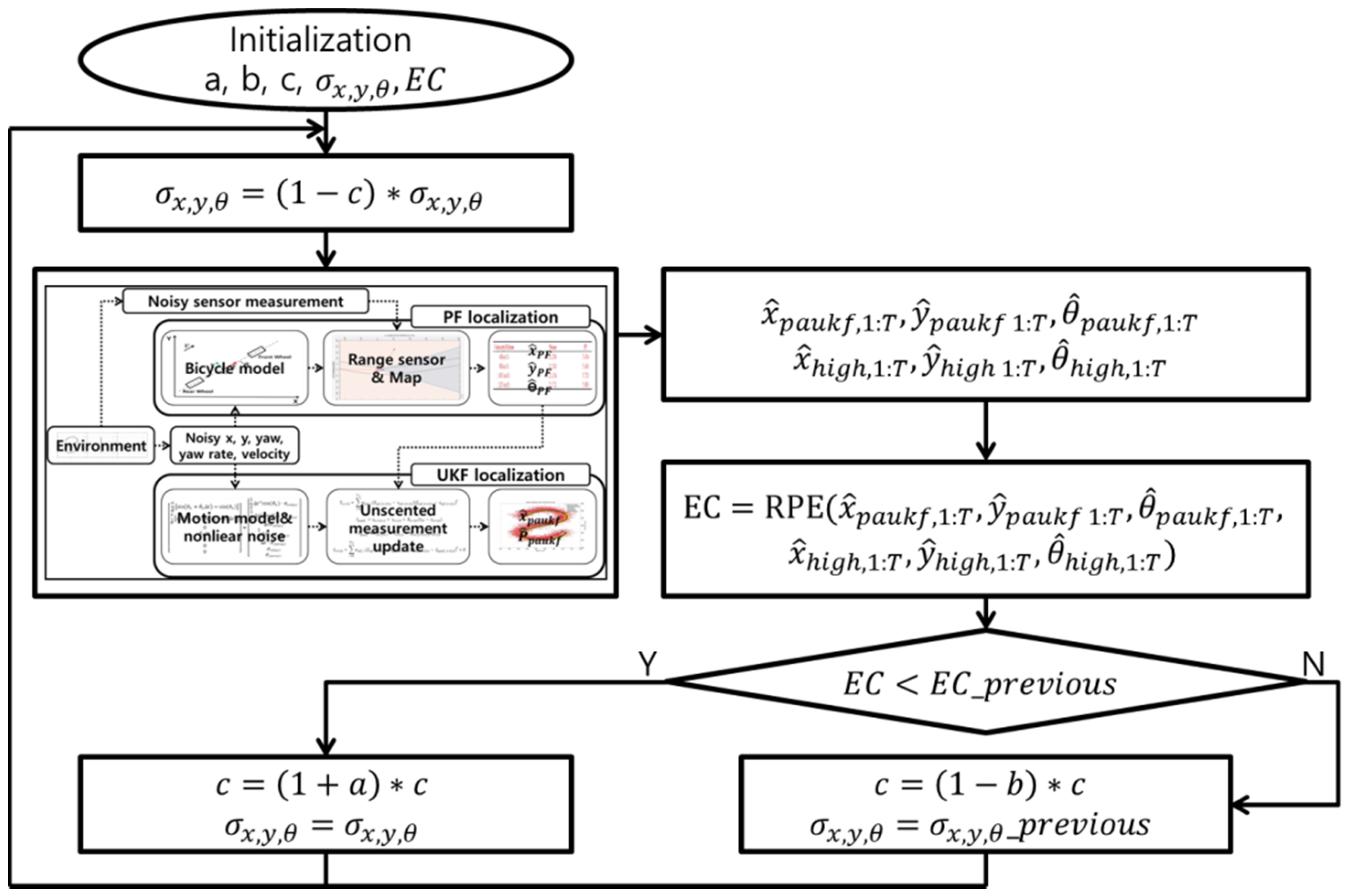
2.2. Discriminative Training of the PAUKF

This section illustrates the implementation of the discriminative training of the PAUKF based on previous research. Although the parameters in both prediction variances and measurement variances could be trained with the same method, in this work we focus on training the measurement variances.

As with most training algorithms, the PAUKF needs to define criteria for evaluating the process. The residual prediction error (RPE) is selected as the evaluation criteria ($\mathrm{EC}$). Not only is it simple to implement but also the performance based on the residual prediction error shows the lowest root mean square (RMS) error according to the work by Abbeel et al. [17]. To calculate the residual prediction error, ground truth data are needed. Since there is no perfect sensor without any noise, a sensor with high accuracy is needed. The high-accuracy measurement can be regarded as the ground truth value with an added random variable $\mathsf{\gamma }$ with zero mean and variance matrix P, like Equations (1) and (2) show. The $\mathrm{h}$ function is the projection of the estimated value onto the highly accurate measurement value. In this paper, we assume the highly accurate sensor could measure the $\mathrm{x}, \mathrm{y}, \mathsf{\theta }$ position directly. Since the algorithm is evaluated in the simulation environment, we could actually use the ground truth value directly. However, the ground truth data are not available in the real world. Therefore, we are trying to evaluate the algorithm in a reasonable environment that is similar to the real world. This is the reason why we do not use the ground truth data as the high-accuracy sensor.

$${\mathrm{z}}_{\mathrm{h}}=h\left(x_{paukf}\right)+\mathsf{\gamma },$$

(1)

$$\mathsf{\gamma } ~ \mathrm{N}\left(0, \mathrm{P}\right),$$

(2)

The residual prediction error is calculated based on the whole data of the high-accuracy measurement ${\mathrm{z}}_{\mathrm{h},1:\mathrm{T}}$ and the estimated value of the PAUKF ${\mathrm{x}}_{\mathrm{paukf},1:\mathrm{T}}$. Since the residual prediction error is based on the estimation result of the PAUKF, it can learn how each variance affects the whole estimation process. Since the purpose of this paper is figuring out the optimal measurement variances $R_{op}$ of the PAUKF, the residual prediction error should be minimized as Equation (3) shows. In Equation (3), $y_t$ is the measurement value from a highly accurate sensor and ${\mu }_t$ is the final estimated result of the PAUKF. The numerical value of ${\mu }_t$ is equal to $x_{paukf}$ in Equation (1). As mentioned in Equation (1), $\mathrm{h}$ is the projection of the PAUKF with a highly accurate measurement value.

$$R_{op}=\underset{R}{\mathrm{argmin}}{{\displaystyle \sum }}_{t=0}^T{\left(y_t-h\left({\mu }_t\right)\right)}^T{P}^{-1}\left(y_t-h\left({\mu }_t\right)\right),$$

(3)

Since it is assumed that the highly accurate sensor could measure the state $\mathrm{x}, \mathrm{y}, \mathsf{\theta }$ directly, the measurement variance matrix becomes an identity matrix. Then, Equation (3) can be simplified as Equation (4). Therefore, the training algorithm should decide the appropriate measurement variance matrix R to make the residual prediction error as small as possible. Since the $x_{paukf,t}$ is the final estimated result of the PAUKF, the evaluation criteria are optimized considering the performance in the whole track.

$$R_{op}=\underset{R}{\mathrm{argmin}}{{\displaystyle \sum }}_{t=0}^T{\left(y_t-h\left(x_{paukf, t} \right)\right)}^2,$$

(4)

As the evaluation criteria of the performance of the PAUKF are well-defined as Equation (4), a training method should be defined. The coordinate descent algorithm is used to minimize the evaluation criteria as in previous research. The training process is simple to implement and intuitively straightforward as shown in Figure 1. ${\mathsf{\sigma }}_{\mathrm{x},\mathrm{y},\mathsf{\theta }}$ is the standard deviation of the measurement, and the alphabetical characters a, b and c are the hyper-parameters of the coordinate descent algorithm. a and b decide the training rate of the coordinate descent and c is a parameter which can increase or decrease the value of the ${\mathsf{\sigma }}_{\mathrm{x},\mathrm{y},\mathsf{\theta }}$ based on the performance of the PAUKF and the value of a and b. If the evaluation criteria (EC) become smaller compared to the previous evaluation criteria (EC_previous), then it means the covariance in the current value makes the PAUKF perform better. So, the training algorithm accepts the new covariance values and continues the training process.

The prediction covariance also can be trained. However, in our research, the simulation environment and algorithm are tested in the simulation. The physical meaning of the precision covariance is the unmodeled vehicle model and unexpected noises. However, since the evaluation environment is a simulation, there are no unmodeled elements of the vehicle and the noises. The prediction covariance can be trained in the same way as training the measurement covariances.

The details of the implementation of the PAUKF training process based on the coordinate descent algorithm are shown in

Table 1. The training process of the PAUKF based on the coordinate descent algorithm.

Order	Process
1	Initialization of hyper-parameters’, $\mathrm{a}, \mathrm{b}, \mathrm{c},{ \mathsf{\sigma }}_{\mathrm{x},\mathrm{y},\mathsf{\theta }},\mathrm{EC}$, training time
2	Start training ${\mathsf{\sigma }}_{\mathrm{x},\mathrm{y},\mathsf{\theta }}$ one by one
3	Calculate the sigma in this iteration
4	Run the PAUKF in the whole track with the calculated sigma
5	Save the data from 1:T of the PAUKF and high-performance sensor
6	Calculate the evaluation criteria based on data collected
7	Compare the performance change
8	Change the training parameters a and b based on the performance
9	Start new training iteration based on the changed training parameters a and b
10	End the iteration if the training process meets training times
11	Save the ${\mathsf{\sigma }}_{\mathrm{x},\mathrm{y},\mathsf{\theta }}$ as the final result

. First, the basic parameters of the training algorithm need to be defined. Then, the PAUKF runs with the computed sigma value in the current iteration. When the algorithm is training one of the standard deviations, the other’s value is fixed. When the vehicle reaches the final position of the track, all the estimated states from the PAUKF and highly accurate measurement values are saved for calculating the residual prediction error. Then, the training algorithm compares the current residual prediction error with the residual prediction error in the previous iteration. If the residual prediction error decreases, the current corresponding measurement standard deviation is accepted. Otherwise, the standard deviation of the measurement should hold the value of the previous iteration. The training process finishes if the iteration meets the training time.

3. Discriminative Training Environment Settings

The training algorithm is based on the MATLAB autonomous driving toolbox. To verify the improvement of the PAUKF with the trained measurement variances, the parameters of vehicle noise and environment noise settings are the same as used in our previous research. The additional parameters are shown in

Table 2. The parameters of the training process.

Parameter Name	Value
Random seed	50
The noise of the high-accuracy sensor	$~\mathrm{N}\left(0, 0.01\right)$
Initial value of ${\mathsf{\sigma }}_{\mathrm{x},\mathrm{y},\mathsf{\theta }}$	10
Initial RPE (m)	9999
Training times	15
a	0.1
b	0.3
Initial c	0.2
Velocity of vehicle (km/h)	60, 70, 80, 90, 100, 110, 120

. The parameters shown in Table 2 are all empirical and can be changed by the researchers who use this algorithm. The random seed of MATLAB is fixed to 50 for the repeatable result. The high accuracy sensor noise is set as zero-mean Gaussian which is a smaller error than other sensors. The initial standard deviation of measurement ${\mathsf{\sigma }}_{\mathrm{x},\mathrm{y},\mathsf{\theta }}$ is set as 10 and the standard deviation decreases based on the coordinate descent algorithm. The initial residual prediction error value is set as 9999 m. The training time is set as 15 based on previous research. The hyper-parameters a, b and c of the coordinate descent algorithm are set as 0.1, 0.3 and 0.2, respectively, based on previous research. The hyper-parameters a and b are constant values and c changes during the training iteration. a and b are empirical parameters that can affect the training rate of the coordinate descent algorithm. The velocities of the training process are varied as 60, 70, 80, 90, 100, 110 and 120 km/h, and the associated evaluations of the performance process are determined.

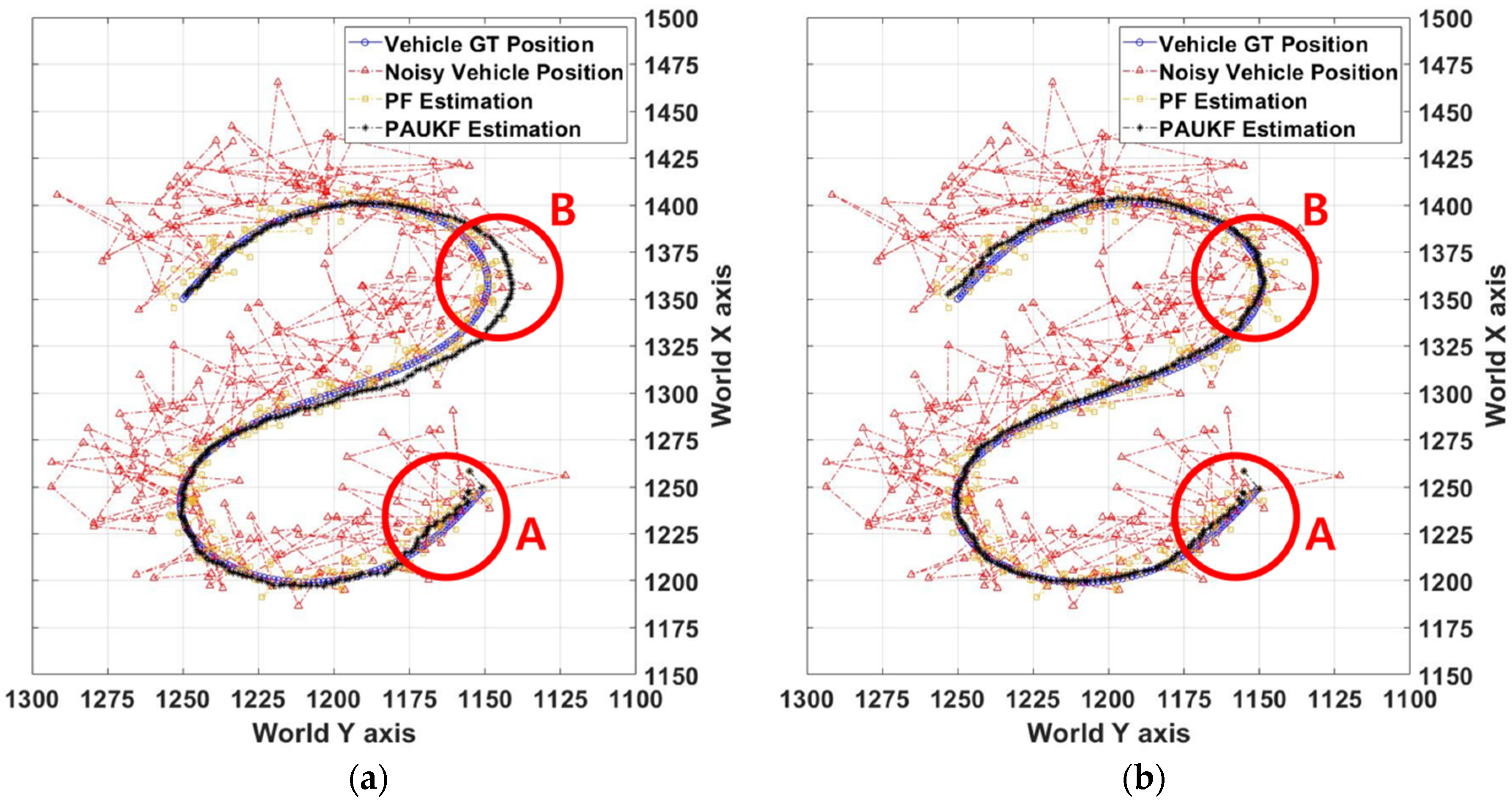
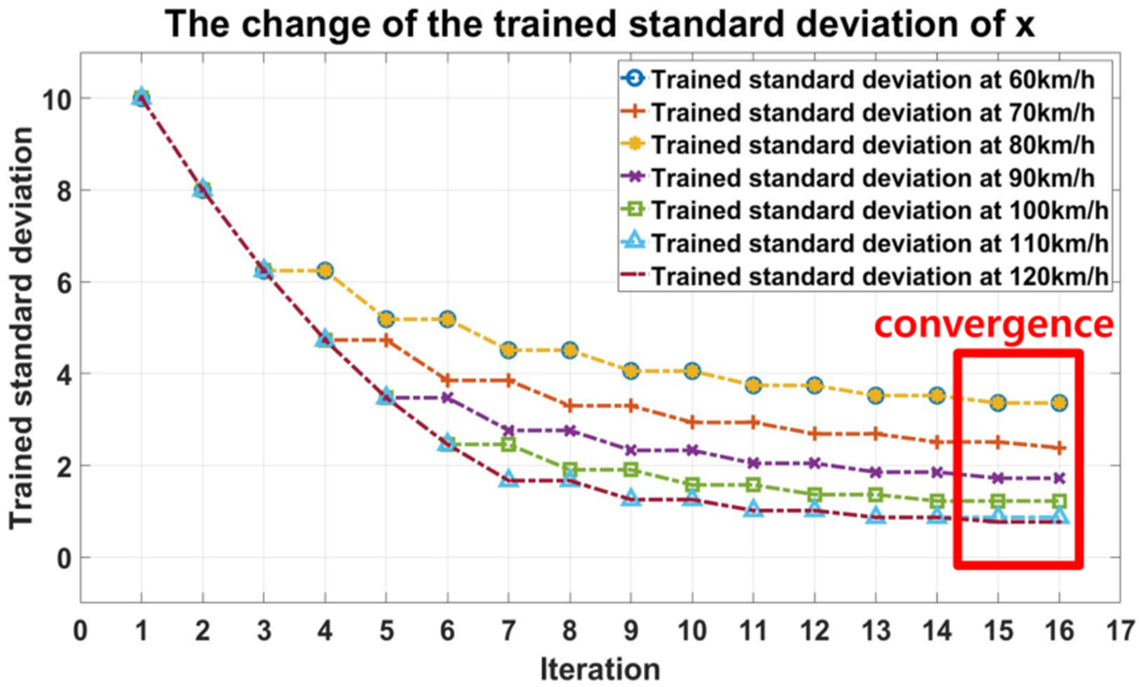
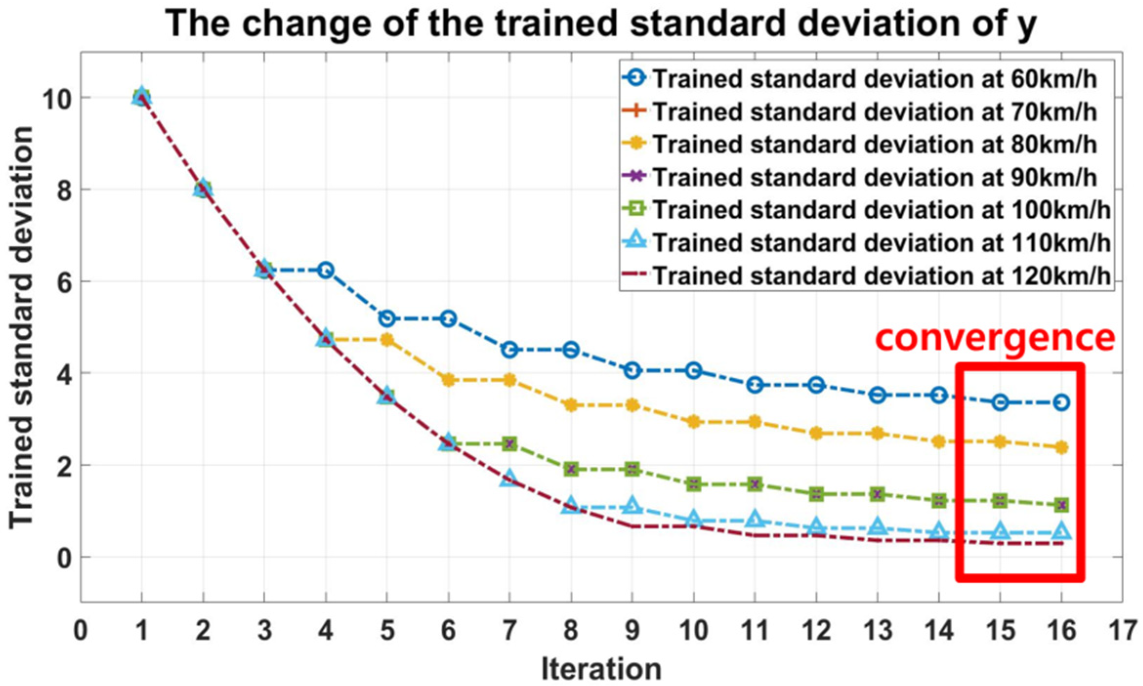
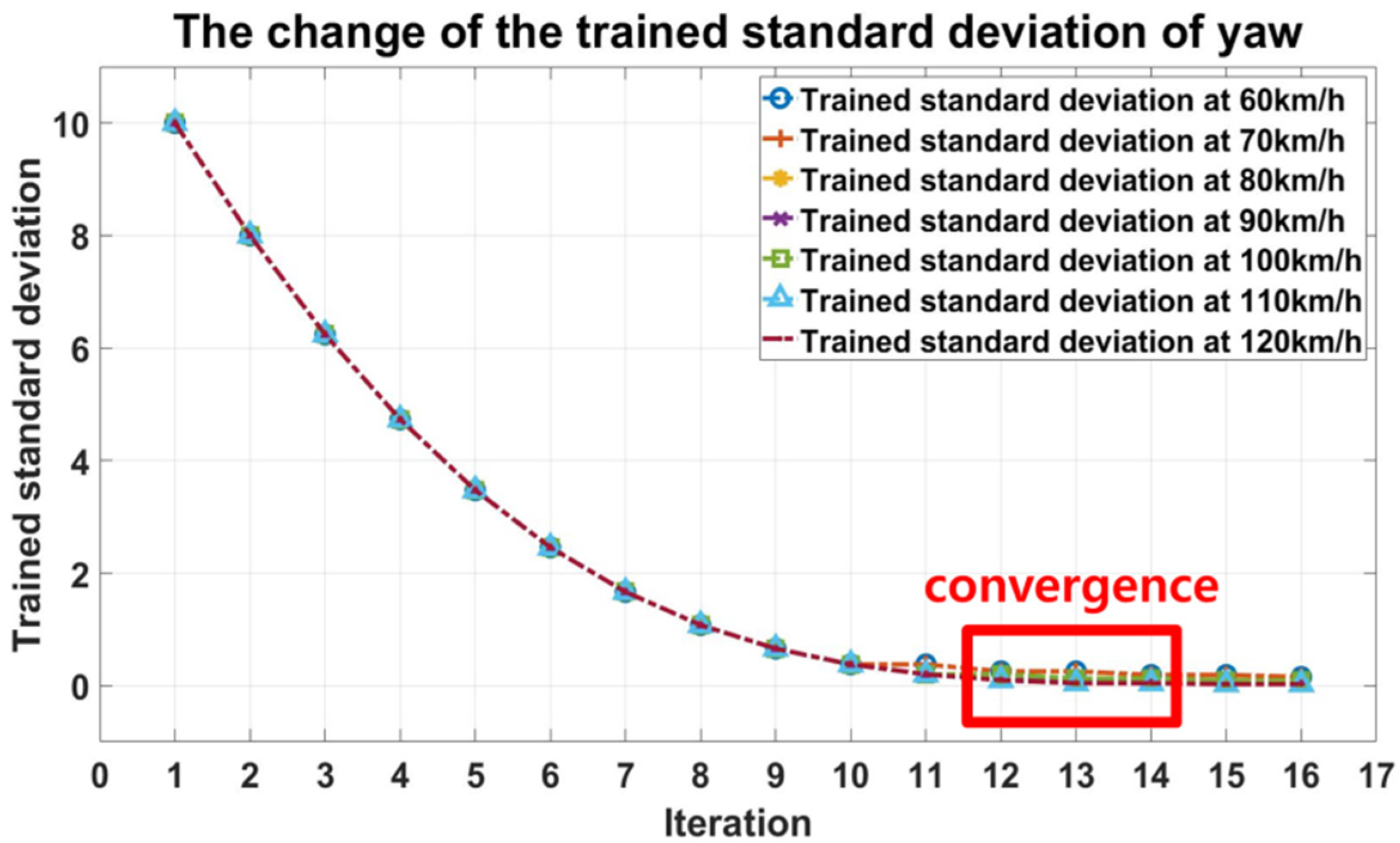
4. The Results of Discriminative Parameter Training of the PAUKF

The simulation experiment results and discussion are given in this section. To evaluate the performance of the manually tuned PAUKF and variance-trained PAUKF, the root mean square error (RMSE) is used as the assessment value. The smaller the value of RMSE, the better the algorithm is. The calculation of the RMSE is shown as Equation (5). The ${\mathrm{RMSE}}_{\mathrm{est}}$ means the RMSE is calculated based on the filter’s estimation and the ${\mathrm{RMSE}}_{\mathrm{noise}}$ is calculated based on the noisy position without filtering. The N represents the number of accumulated position data after the vehicle runs on the whole track.

$$\left[\begin{array}{c}{\mathrm{RMSE}}_{\mathrm{est}}\\ {\mathrm{RMSE}}_{\mathrm{noise}}\end{array}\right]=\left[\begin{array}{c}\sqrt{[{{\displaystyle \sum }}_{\mathrm{i}=1}^{\mathrm{N}}{\left({\mathrm{Position}}_{{\mathrm{est}}_{\mathrm{i}}}-{\mathrm{Position}}_{{\mathrm{mean}}_{\mathrm{est}}{}_{\mathrm{i}}}\right)}^2]/\mathrm{N}}\\ \sqrt{[{{\displaystyle \sum }}_{\mathrm{i}=1}^{\mathrm{N}}{\left({\mathrm{Position}}_{{\mathrm{noise}}_{\mathrm{i}}}-{\mathrm{Position}}_{{\mathrm{mean}}_{\mathrm{noise}}{}_{\mathrm{i}}}\right)}^2]/\mathrm{N}}\end{array}\right],$$

(5)

Figure 2 is the filtering result of the manually tuned PAUKF and the trained PAUKF at 120 km/h. Figure 2a is the trajectory of the noisy vehicle position, estimated by the PF, and the manually tuned PAUKF. Figure 2b is the trajectory of the noisy vehicle position estimated by the PF, and the PAUKF with the trained measurement variance. The blue line with the blue circles is the ground truth position of the vehicle, the red dashed line with the red triangles is the noisy GPS sensor measured position, the yellow dash line with the yellow squares is the estimation result of the PF and the black dash line with the black asterisks is the final estimation result of the PAUKF. The estimation results of the manually tuned PAUKF and the variance-trained PAUKF have many differences. From the figure, the algorithm with trained variance has better performance in the whole track. The most significant differences are marked with red circle A and red circle B for comparison. Red circle A shows the estimation results of the vehicle at the start. The vehicle localizes itself quickly in both of the figures. However, the error of estimation in (a) becomes larger than the error in (b). Since the parameters and random seed are fixed, the performance of the PF and UKF does not change, meaning that the only reason for the divergent performances is the weight of the measurement which is decided on the measurement variances in the PAUKF. Compared to the manually tuned PAUKF, the estimation error of the variance-trained PAUKF is smaller and smoother. The performance of the PAUKF becomes more distinct at circle B. The manually tuned PAUKF tends to put more weight on the prediction model. However, not only does the prediction model not describe the physical movement, but the values used in the prediction contain a lot of noise. Due to the non-optimized measurement variances, the algorithm cannot balance the information well. As a result, the PAUKF cannot fully use the information from the PF which provides an accurate measurement based on map matching. Due to the non-optimized variance value, the position error of the manually tuned PAUKF is larger than the error of the variance-trained PAUKF at circle B.

The results of the RMSE of the filter at different velocities are shown in

Table 3. RMSE of the basic extended PAUKF and trained PAUKF (unit: m).

	Position of Vehicle		PF		PAUKF
Parameter	Manual	Trained	Manual	Trained	Manual	Trained
60 km/h	29.465	29.465	6.317	6.317	2.478	2.651
70 km/h	29.351	29.351	6.238	6.238	1.767	1.510
80 km/h	28.319	28.319	6.265	6.265	2.303	2.645
90 km/h	29.919	29.919	5.861	5.861	2.169	2.270
100 km/h	29.981	29.981	6.324	6.324	2.833	2.166
110 km/h	29.144	29.144	6.303	6.303	3.441	2.574
120 km/h	30.072	30.072	6.098	6.098	3.881	2.093
Mean	29.465	29.465	6.201	6.201	2.696	2.273
RMSE Change	0%		0%		−15.70%

. The title “position of vehicle” means the RMSE of the noisy position of the vehicle. The title “manual” means the data are generated by the manually tuned PAUKF. The title “trained” means the data are generated with variance-trained PAUKF. The “Mean” means the average of the RMSE of different velocity conditions and the “RMSE change” means the difference in the RMSE of the manually tuned PAUKF and the variance-trained PAUKF. As illustrated in Section 3, the parameters used in the trained variance PAUKF are the same as manually tuned PAUKF, meaning the only variable making the result change is the value of the measurement variance. The RMSE which is calculated based on the second row of Equation (5) shows that both the manually tuned PAUKF and variance-trained PAUKF are tested under the same noisy environment, and the RMSE of the manually tuned PF and trained PF shows the same value. This means the training process does not affect the performance of the PF. As a result, the parameter “RMSE change” in the title “position of vehicle” is equal to 0%. The change in the RMSE happens at the PAUKF column. The RMSE of the PF and PAUKF is calculated based on the first row of Equation (5). Compared to the manually tuned PAUKF, the RMSE of the variance-trained PAUKF decreases about 15.7% on average only because of the well-trained measurement covariance values. The RMSE results show that the trained variance PAUKF improves the performance without adding any computational burden.

The numerical value of measurement variances affects the estimation performance, as seen from the results. The variance is trained by the coordinate descent algorithm in 15 iterations of each parameter. In the training algorithm, the variance of $\mathrm{x}, \mathrm{y},$ and $\mathsf{\theta }$ is calculated by the standard deviation. Therefore, Figure 3, Figure 4 and Figure 5 show the record of the standard deviation of $\mathrm{x}, \mathrm{y},$ and $\mathsf{\theta }$. Since the initial measurement variance is equal to 10, the PAUKF tends to give greater weight to the prediction model than to the measurement. From Figure 3, the standard deviation of x converged at iteration 15–16. The final standard deviation converges to different values at different velocities. The reason for this phenomenon is the noise in the prediction model decreasing the precision of the estimation. Therefore, the error of the prediction model of the PAUKF becomes larger. Conversely, the estimation of the PF is not affected by the velocity of the vehicle, meaning the PAUKF should give more weight to the PF estimation. The smaller the standard deviation of the measurement, the more credence the PAUKF gives to the measurement value. So, the weight of the PF is represented as the standard deviation and the standard deviation decreases as the velocity increases, as shown in Figure 3. The standard deviation of y shows the same property of the standard deviation of x, as shown in Figure 4.

Figure 5 shows the standard deviation change of the yaw angle in the training iteration. The standard deviation change of the yaw angle differs from that of x and y in that it is almost the same in all velocity conditions. In the training process, therefore, the performance of the PAUKF improves as the weight of the yaw angle measurement increases. The yaw angle, which is estimated from the PF, has higher precision than the on-board sensor in all velocity conditions. This also means that the manually tuned variance is not optimal enough. The convergence of the yaw angle happens at iteration 12–14.

5. Conclusions

In this paper, we present a discriminative parameter training methodology of the PAUKF. The coordinate descent algorithm is used for learning the optimal measurement variances and the residual prediction error is used for evaluating the performance of the extended PAUKF. The performance of the trained variance-based PAUKF is verified by using the simulation environment. By comparing the RMSE of the variance-trained PAUKF and the manually tuned PAUKF, the trained variance-based PAUKF demonstrates improvement in the precision of about 15.7%. Since the training process is done offline, the PAUKF improves the precision without any extra online computational burden. By using our training method, researchers not only reduce the time cost but also could achieve a more precise location of the self-driving car by the aid of trained parameters. In the future, we will implement the extended PAUKF into the four-wheel ground vehicle in the real world.

References

1. Rezaei, S.; Sengupta, R. Kalman filter-based integration of DGPS and vehicle sensors for localization. IEEE Trans. Control Syst. Technol. 2007, 15, 1080–1088. [Google Scholar] [CrossRef] [Green Version]
2. Bakkali, W.; Kieffer, M.; Lalam, M.; Lestable, T. Kalman filter-based localization for Internet of Things LoRaWANTM End Points. In Proceedings of the IEEE International Symposium on Personal, Indoor and Mobile Radio Communications, PIMRC, Montreal, QC, Canada, 8–13 October 2017; pp. 1–6. [Google Scholar]
3. Yang, Q.; Taylor, D.G.; Durgin, G.D. Kalman filter based localization and tracking estimation for HIMR RFID systems. In Proceedings of the 12th Annual IEEE International Conference on RFID, RFID 2018, Orlando, FL, USA, 10–12 April 2018; pp. 1–5. [Google Scholar]
4. Cong, T.H.; Kim, Y.J.; Lim, M.T. Hybrid Extended Kalman Filter-based localization with a highly accurate odometry model of a mobile robot. In Proceedings of the 2008 International Conference on Control, Automation and Systems, ICCAS 2008, Seoul, Korea, 14–17 October 2008; pp. 738–743. [Google Scholar]
5. Lu, J.; Li, C.; Su, W. Extended Kalman filter based localization for a mobile robot team. In Proceedings of the Proceedings of the 28th Chinese Control and Decision Conference, CCDC 2016, Yinchuan, China, 28–30 May 2016; pp. 939–944. [Google Scholar]
6. Reina, G.; Vargas, A.; Nagatani, K.; Yoshida, K. Adaptive Kalman filtering for GPS-based mobile robot localization. In Proceedings of the SSRR2007—IEEE International Workshop on Safety, Security and Rescue Robotics Proceedings, Rome, Italy, 27–29 September 2007. [Google Scholar]
7. Subhan, F.; Hasbullah, H.; Ashraf, K. Kalman filter-based hybrid indoor position estimation technique in bluetooth networks. Int. J. Navig. Obs. 2013, 2013, 570964. [Google Scholar] [CrossRef] [Green Version]
8. Ullah, I.; Shen, Y.; Su, X.; Esposito, C.; Choi, C. A Localization Based on Unscented Kalman Filter and Particle Filter Localization Algorithms. IEEE Access 2020, 8, 2233–2246. [Google Scholar] [CrossRef]
9. Chen, S.Y. Kalman filter for robot vision: A survey. IEEE Trans. Ind. Electron. 2012, 59, 4409–4420. [Google Scholar] [CrossRef]
10. Pomarico-Franquiz, J.J.; Shmaliy, Y.S. Accurate self-localization in rfid tag information grids using fir filtering. IEEE Trans. Ind. Inform. 2014, 10, 1317–1326. [Google Scholar] [CrossRef]
11. Loebis, D.; Sutton, R.; Chudley, J.; Naeem, W. Adaptive tuning of a Kalman filter via fuzzy logic for an intelligent AUV navigation system. Control Eng. Pract. 2004, 12, 1531–1539. [Google Scholar] [CrossRef]
12. Chung, H.Y.; Hou, C.C.; Chen, Y.S. Indoor Intelligent Mobile Robot Localization Using Fuzzy Compensation and Kalman Filter to Fuse the Data of Gyroscope and Magnetometer. IEEE Trans. Ind. Electron. 2015, 62, 6436–6447. [Google Scholar] [CrossRef]
13. Krishnan, R.G.; Shalit, U.; Sontag, D. Deep Kalman Filters. In Proceedings of the NIPS 2016 Workshop: Advances in Approximate Bayesian Inference, Barcelona, Spain, 9 December 2016; pp. 1–7. [Google Scholar]
14. Hosseinyalamdary, S. Deep Kalman filter: Simultaneous multi-sensor integration and modelling; A GNSS/IMU case study. Sensors 2018, 18, 1316. [Google Scholar] [CrossRef] [PubMed] [Green Version]
15. Lin, M.; Yoon, J.; Kim, B. Self-Driving Car Location Estimation Based on a Particle-Aided Unscented Kalman Filter. Sensors 2020, 20, 2544. [Google Scholar] [CrossRef] [PubMed]
16. Lin, M.; Kim, B. Extended Particle-Aided Unscented Kalman Filter Based on Self-Driving Car Localization. Appl. Sci. 2020, 10, 5045. [Google Scholar] [CrossRef]
17. Abbeel, P.; Coates, A.; Montemerlo, M.; Ng, A.Y.; Thrun, S. Discriminative training of kalman filters. Robot. Sci. Syst. 2005, 2, 1. [Google Scholar]
18. Sakai, A.; Kuroda, Y. Discriminative parameter training of Unscented Kalman Filter. IFAC Proc. Vol. 2010, 43, 677–682. [Google Scholar] [CrossRef]
Figure 1. Flowchart of the training process of the extended particle-aided unscented Kalman filter (PAUKF) based on the coordinate descent algorithm.
Applsci 10 06260 g001
Figure 2. The position estimation results of the PAUKF. (a) The position estimation result of the PAUKF with manually tuned variance; (b) the position estimation result of the PAUKF with trained variance.
Applsci 10 06260 g002
Figure 3. The change of the trained variance of x in the training iteration.
Applsci 10 06260 g003
Figure 4. The change of the trained variance of y in the training iteration.
Applsci 10 06260 g004
Figure 5. The change of the trained variance of the yaw angle in the training iteration.
Applsci 10 06260 g005