Extended Particle-Aided Unscented Kalman Filter Based on Self-Driving Car Localization

Abstract

The location of the vehicle is a basic parameter for self-driving cars. The key problem of localization is the noise of the sensors. In previous research, we proposed a particle-aided unscented Kalman filter (PAUKF) to handle the localization problem in non-Gaussian noise environments. However, the previous basic PAUKF only considers the infrastructures in two dimensions (2D). This previous PAUKF 2D limitation rendered it inoperable in the real world, which is full of three-dimensional (3D) features. In this paper, we have extended the previous basic PAUKF’s particle weighting process based on the multivariable normal distribution for handling 3D features. The extended PAUKF also raises the feasibility of fusing multisource perception data into the PAUKF framework. The simulation results show that the extended PAUKF has better real-world applicability than the previous basic PAUKF.

1. Introduction

In recent years, the self-driving car has become the hottest topic in the automotive industry [1,2,3,4]. To make a self-driving car drive conveniently and safely, accurate identification of the vehicle’s position is one of the most important parameters. Only if the self-driving car knows where it is can it execute the next decision. Localization is on the basic module of the perception module. Almost all the other data work on the basis of the location data. The most commonly used localization method is GPS [5]. However, GPS signals are affected by the quantity of satellites and by the multipath effect in an urban environment [6,7,8]. When GPS cannot obtain a sufficient quantity of satellites [9], an alternative approach to localization is needed. As high-definition (HD) maps have developed, it has become possible to localize the vehicle position based on map matching [10,11]. However, not only does the HD map make a noise, but the sensors have a detect noise as well. A method is needed, therefore, to filter noise from different sources. The Kalman filter family is generally used to filter the noise of many sensors [12,13,14]. The Kalman filter is designed for processing Gaussian noise with a linear transition model and a linear measurement model. However, in the real world, most of the transitions and measurements are not linear. Therefore, the extended Kalman filter (EKF) and unscented Kalman filter (UKF) were proposed [15,16,17,18,19,20] to provide a methodology to handle nonlinear transitions and measurements. EKF and UKF still operate on a basic assumption of the Kalman filter, in that the noise always should be Gaussian. The particle filter (PF) is a Monte Carlo-based method that can handle any type of noise [21,22,23,24,25]. The more particles used, the more accurate PF can be. However, because the PF method involves calculating each particle’s weight, the precision and computational burden must trade-off.

In our previous work, we proposed the particle-aided unscented Kalman filter (PAUKF), which has more stable and precise performance compared to the PF using the unscented Kalman filter [26]. We constructed the PAUKF using the infrastructure two-dimensional information in previous research. The mean estimation error for the PAUKF is 1.08 m and its variance is 0.7147 m, which is more precise than the mean of 1.69 m and variance of 1.63 m obtained by GANGNAM for a similar noise environment. However, in the real world, there is rich 3D information gained from perception module sensors that use light detection and ranging (LiDAR), and radio detection and ranging (RADAR). The PAUKF algorithm only considers two-dimensional features; it cannot process features in three dimensions appropriately. The PAUKF algorithm needs extended capabilities to handle three-dimensional information.

In this paper, we have improved the perception calculation method and extended the weight calculation scheme, by using a multivariable normal distribution in three dimensions. Compared to our previous research, the extended PAUKF improves the particle selection method. With an improved particle weighting scheme, the extended PAUKF extracts a more precise global location based on 3D features. We also found that the extended PAUKF provides feasibility to fuse multisource perception data into the PAUKF framework by weighting the particles. The simulation result shows that the extended PAUKF achieves better performance in a three-dimensional feature environment compared to the previous PAUKF. The extended PAUKF improves precision 73.81% compared to the initial PAUKF. The limitations of this algorithm are that the hyperparameters are not optimal even when tuned carefully, and that it does not consider the vehicle on the freeway on-ramps. These limitations should be mitigated in future research.

Section 2 illustrates the extension of the basic PAUKF to incorporate three-dimensional features and the framework to fuse multisource perception data. Section 3 illustrates the simulation environment. Section 4 shows the results of simulation and provides a discussion of the extended PAUKF’s performance compared to that of the basic PAUKF.

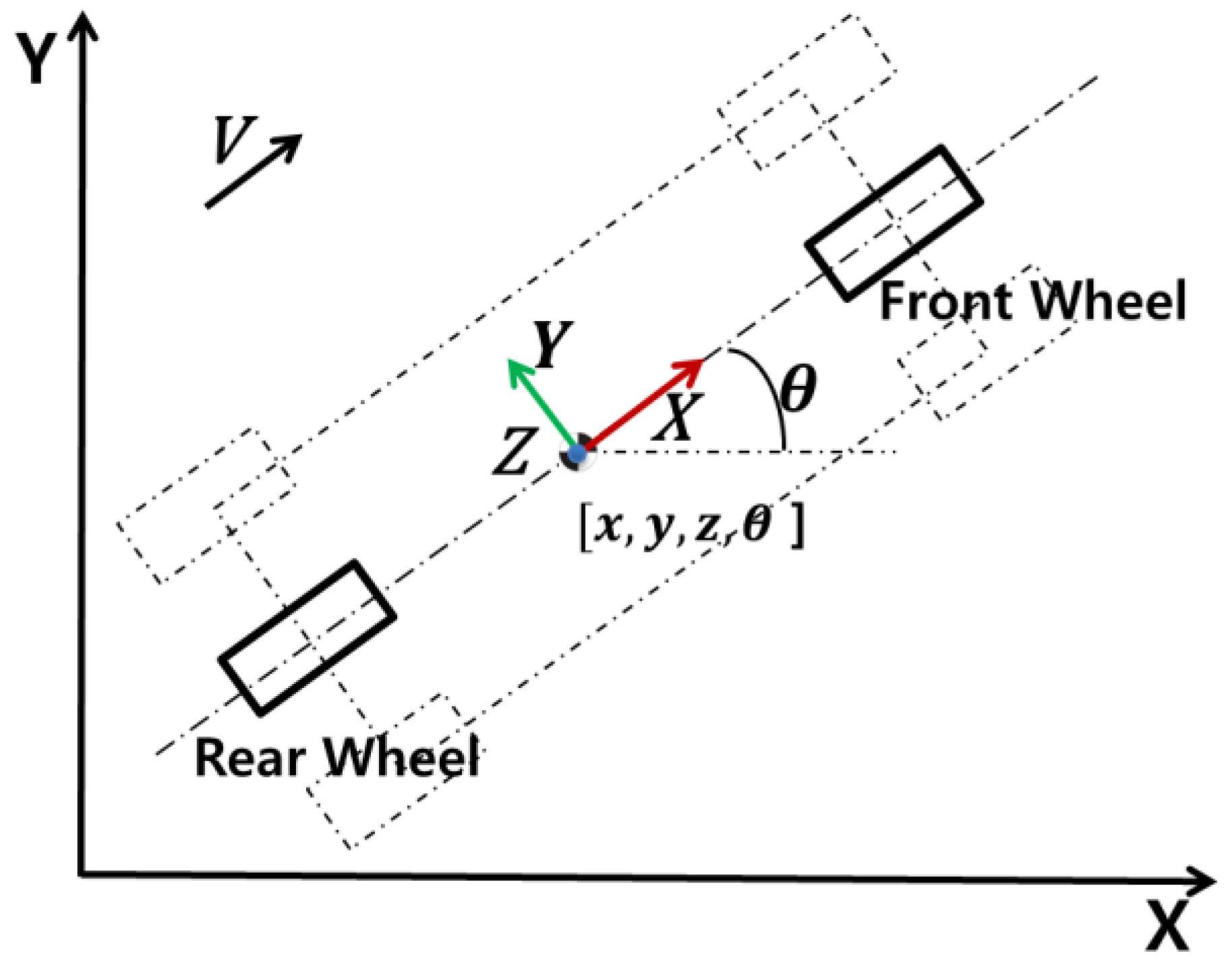
2. Extended Particle-Aided Unscented Kalman Filter

This section describes the implementation of the extended PAUKF. As is assumed with the initial PAUKF, the environment was taken as Markov, meaning that the current state depends only on the previous state. A bicycle model was used for making a prediction model of particles, as is shown in Figure 1. We assumed that the changes in steering and slip angle information were included in the yaw angle. From the XY plane, outside of the page, is the positive Z direction.

This study follows all the assumptions defined in the previous basic PAUKF. The extended algorithm is the particle filter portion. The unscented Kalman filter part is the same as that used with the previous basic PAUKF.

2.1. Particle Filter Initialization

Initialization provides the initial guess of the ego vehicle’s position in global coordinates via GPS. Once an algorithm knows the initial guess, it randomly generates some particles based on the initial position. If the algorithm is run in an indoor environment, an initial guess of the global map-based position should be given. In the PAUKF algorithm framework, an initial guess is not necessary per se, since features in the HD map provides a relative global position, but having one can make the estimated result converge to the ground truth more rapidly.

2.2. Particle Prediction

The prediction step predicts the state one timestamp ahead of the current state. According to Bayesian rule, the prediction always refers to the prior belief. It provides prior information of the vehicle based on the previous posterior belief, which is often the final estimated result of the previous timestamp. In this research, the road was assumed to be a flat XY plane, and movement in the vertical direction z was considered random noise. The state vector is given as Equation (1) and the vertical direction movement is given as Equation (2). Here, the value of ${\mathsf{\sigma }}_{{\mathrm{v}}_{\mathrm{z}}}$ is 0.3.

$$\mathrm{X}=\left[\mathrm{x}, \mathrm{y}, \mathrm{z}, \mathsf{\theta }\right],$$

(1)

$${\mathrm{z}}_{\mathrm{v}} ~ \mathrm{N}\left(0,{ \mathsf{\sigma }}_{{\mathrm{v}}_{\mathrm{z}}}^2\right).$$

(2)

Equation (3) shows the transition model of the particles. Each particle is generated randomly and calculates the next timestamp value based on the transition model. The predicted value provides the prior guess of each particle and all the particles will be weighted based on the predicted value and current measurement value [27].

$${\overline{\mathrm{X}}}_{\mathrm{k}+1}={\left[\begin{array}{c}\overline{\mathrm{x}}\\ \overline{\mathrm{y}}\\ \overline{\mathrm{z}}\\ \overline{\mathsf{\theta }}\end{array}\right]}_{\mathrm{k}+1}=\left[\begin{array}{c}\frac{{\mathrm{v}}_{\mathrm{k}}}{\dot{{\mathsf{\theta }}_{\mathrm{k}}\left(\Delta \mathrm{t}\right)}}\left[\sin \left({\mathsf{\theta }}_{\mathrm{k}}+\dot{{\mathsf{\theta }}_{\mathrm{k}}\left(\Delta \mathrm{t}\right)}\right)-\sin \left({\mathsf{\theta }}_{\mathrm{k}}\right)\right]\\ \frac{{\mathrm{v}}_{\mathrm{k}}}{\dot{{\mathsf{\theta }}_{\mathrm{k}}\left(\Delta \mathrm{t}\right)}}\left[\cos \left({\mathsf{\theta }}_{\mathrm{k}}\right)-\cos \left({\mathsf{\theta }}_{\mathrm{k}}+\dot{{\mathsf{\theta }}_{\mathrm{k}}\left(\Delta \mathrm{t}\right)}\right)\right]\\ {\mathrm{z}}_{\mathrm{v},\mathrm{k}+1}\\ \dot{{\mathsf{\theta }}_{\mathrm{k}}\left(\Delta \mathrm{t}\right)}\end{array}\right]+{\left[\begin{array}{c}\mathrm{x}\\ \mathrm{y}\\ 0\\ \mathsf{\theta }\end{array}\right]}_{\mathrm{k}}.$$

(3)

When the yaw rate equals zero, Equation (3) can be shown to become infinite. A different prediction model should therefore be used when the yaw rate is zero as shown in Equation (4).

$${\overline{\mathrm{X}}}_{\mathrm{k}+1}={\left[\begin{array}{c}\overline{\mathrm{x}}\\ \overline{\mathrm{y}}\\ \overline{\mathrm{z}}\\ \overline{\mathsf{\theta }}\end{array}\right]}_{\mathrm{k}+1}=\left[\begin{array}{c}{\mathrm{v}}_{\mathrm{k}}\cos \left({\mathsf{\theta }}_{\mathrm{k}}\right)\Delta \mathrm{t}\\ {\mathrm{v}}_{\mathrm{k}}\sin ({\mathsf{\theta }}_{\mathrm{k}})\Delta \mathrm{t}\\ {\mathrm{z}}_{\mathrm{v},\mathrm{k}+1}\\ 0\end{array}\right]+{\left[\begin{array}{c}\mathrm{x}\\ \mathrm{y}\\ 0\\ \mathsf{\theta }\end{array}\right]}_{\mathrm{k}}$$

(4)

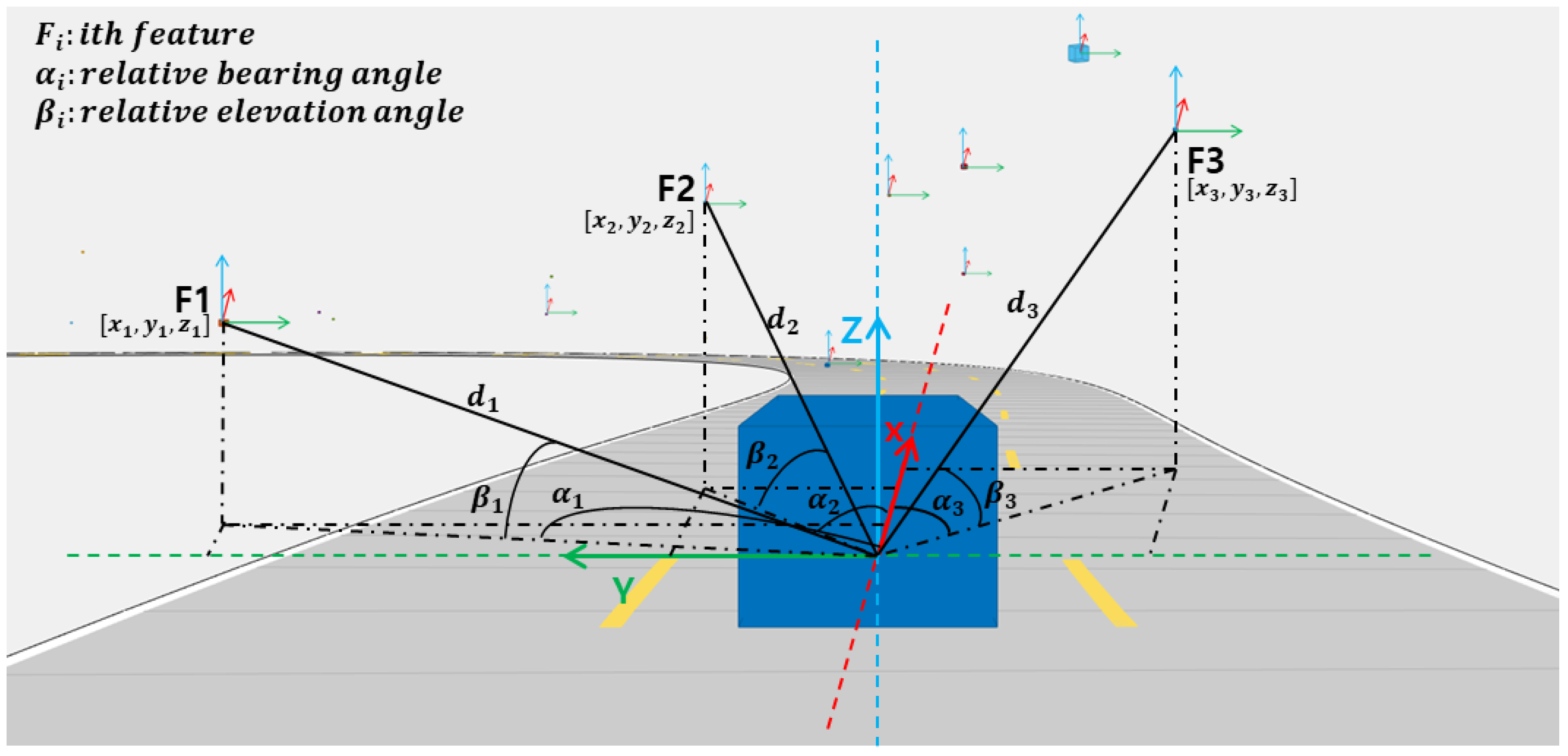
2.3. Particle Weight Estimation Based on Three-Dimensional Features

Weight estimation, also known as sequential importance sampling (SIS), is a critical step in that it directly affects the importance of each particle from the prediction step. The particle filter is an application of an SIS approach. The main idea of weight estimation is to represent the required posterior density function by a set of random samples, which are taken from the prediction step. These samples use associated weights to compute estimates based on these samples and weights [28].

It is necessary to calculate the error of the predicted mean value and the measured value of each particle, in order to calculate the weight. On the basis of the error of predicted and measured values, the weight of each particle can be calculated. Since the predicted value is calculated in the prediction step, the only parameter that affects weight is the measurement value. In this paper, the extended PAUKF considered the three-dimensional features from the perception module, such as LiDAR- and RADAR-based object recognition. Since the range sensor calculated the distance ${\mathrm{d}}_{\mathrm{i}}$ between features based on time of flight, the measured distance is the point-to-point distance, as Figure 2 shows. The method differs from the two-dimensional case. Because of the vertical offset of the features, the weight calculation should also be extended to a higher dimension. The only known measurement values are the point-to-point relative distance ${\mathrm{d}}_{\mathrm{i}}$ between vehicle and feature F as well as the angle of the relative bearing ${\mathsf{\alpha }}_{\mathrm{i}}$ and relative elevation ${\mathsf{\beta }}_{\mathrm{i}}$, as Figure 2 shows. The geometry perception data should be considered as well as the noise affection in the vertical direction.

The measurement value of the vehicle is shown as Equation (5), since sensors in the real world cannot precisely recognize out-ranged targets. Therefore, a valid recognition limit of 50 m was set, meaning that the vehicle localizes itself based on features within 50 m.

$$\begin{gathered} {\mathrm{If} \mathrm{d}}_{\mathrm{i}}<50,{\hspace{1em}\mathrm{Z}}_{\mathrm{k}+1 }={\left[\begin{array}{c}{\mathrm{d}}_{\left[\mathrm{i}\right]}\\ \Delta {\mathsf{\alpha }}_{\left[\mathrm{i}\right]}\end{array}\right]}_{\mathrm{k}+1}= \\ {\left[\begin{array}{c}\sqrt{{\left({\mathrm{x}}_{\mathrm{f}\_\mathrm{i},\mathrm{k}+1}-{\mathrm{x}}_{\mathrm{v}}\right)}^2+{\left({\mathrm{y}}_{\mathrm{f}\_\mathrm{i},\mathrm{k}+1}-{\mathrm{y}}_{\mathrm{v}}\right)}^2+{\left({\mathrm{z}}_{\mathrm{f}\_\mathrm{i},\mathrm{k}+1}-{\mathrm{z}}_{\mathrm{v}}\right)}^2}\\ \arctan \left(\frac{{\mathrm{x}}_{\mathrm{f}\_\mathrm{i},\mathrm{k}+1}-{\mathrm{x}}_{\mathrm{v}}}{{\mathrm{y}}_{\mathrm{f}\_\mathrm{i},\mathrm{k}+1}-{\mathrm{y}}_{\mathrm{v}}}\right)\end{array}\right]}_{\mathrm{k}+1}+{\left[\begin{array}{c}{ϵ}_{\mathrm{d}}\\ -{ \mathsf{\theta }}_{\mathrm{v}}+{ϵ}_{\Delta \mathsf{\alpha }}\end{array}\right]}_{\mathrm{k}+1}. \end{gathered}$$

(5)

The perception values are transformed based on the generated particle value ${\overline{\mathrm{X}}}_{\mathrm{k}+1}$, which is represented as ${\overline{\mathrm{x}}}_{\mathrm{f},\mathrm{k}+1}$, ${\overline{\mathrm{y}}}_{\mathrm{f},\mathrm{k}+1}$ and ${\overline{\mathrm{z}}}_{\mathrm{f},\mathrm{k}+1}$. As the feature extends to three dimensions, an extended method should be used to evaluate each weight. After unifying the measurement value and the predicted value in map coordinates, the multivariable normal distribution was used for weighting particles, as Equation (6) shows. The highest weighted particle was used for estimating the position. The total particle number N is 100.

$$\begin{gathered} {\mathrm{w}}_{\mathrm{i}}=\mathrm{P}\left({\mathrm{x}}_{\mathrm{p},\mathrm{i}},{\mathrm{y}}_{\mathrm{p},\mathrm{i}},{\mathrm{z}}_{\mathrm{p},\mathrm{i}}\right) \\ =\frac{1}{{\left(2\mathsf{\pi }\right)}^{\frac{3}{2}}{\mathsf{\sigma }}_{\mathrm{x}}{\mathsf{\sigma }}_{\mathrm{y}}{\mathsf{\sigma }}_{\mathrm{z}}}{\mathrm{e}}^{-\left(\frac{{\left({\overline{\mathrm{x}}}_{\mathrm{f}\_\mathrm{i},\mathrm{k}+1}-{\mathsf{\mu }}_{\mathrm{f},\mathrm{x}}\right)}^2}{2{\mathsf{\sigma }}_{\mathrm{x}}^2}+\frac{{\left({\overline{\mathrm{y}}}_{\mathrm{f}\_\mathrm{i},\mathrm{k}+1}-{\mathsf{\mu }}_{\mathrm{f},\mathrm{y}}\right)}^2}{2{\mathsf{\sigma }}_{\mathrm{y}}^2}+\frac{{\left({\overline{\mathrm{z}}}_{\mathrm{f}\_\mathrm{i},\mathrm{k}+1}-{\mathsf{\mu }}_{\mathrm{f},\mathrm{z}}\right)}^2}{2{\mathsf{\sigma }}_{\mathrm{z}}^2}\right)}, \mathrm{i}=1, 2, 3 \dots \mathrm{N}. \end{gathered}$$

(6)

On the basis of the multivariable distribution framework, if there are different sources of perception data, they can be fused simply. When the vehicle receives multiple perception data about one feature, the belief of each perception data can be calculated based on the multivariable normal distribution equation, as Equation (6) shows. After calculating the probability based on each sensor, the final weight of each particle can be calculated, as Equation (7) shows. This provides a feasible multisource data fusion method based on the PAUKF. Please note that the feasibility is not verified. In this paper, we only considered the single range sensor case.

$${\mathrm{w}}_{\mathrm{i}}={\mathrm{P}}_{\mathrm{LiDAR}}\left(\mathrm{x},\mathrm{y},\mathrm{z}\right){\ast \mathrm{P}}_{\mathrm{RADAR}}\left(\mathrm{x},\mathrm{y},\mathrm{z}\right){\ast \mathrm{P}}_{\mathrm{Camera}}\left(\mathrm{x},\mathrm{y},\mathrm{z}\right)\ast \dots {\mathrm{P}}_{\mathrm{perception} \mathrm{source}}\left(\mathrm{x},\mathrm{y},\mathrm{z}\right).$$

(7)

2.4. Resampling Particles

The resampling step tries to eliminate samples with low importance weights. As long as the importance weight is low, the particle’s value effect is small. In this paper, we only considered the precision of the filter; therefore, the algorithm resampling happens at every timestamp. The highest weight of the particle’s value was considered as the final estimated value.

2.5. UKF Part of Extended PAUKF

In previous research, we found that the PF estimated result is not smooth and stable. The UKF uses the PF estimated results, which can make the estimated result more stable and precise. In this paper, we optimized the geometry of perception and extended the weight calculation method based on the multinomial normal distribution equation, meaning that the UKF received more precise $\left[\mathrm{x}, \mathrm{y}, \mathsf{\theta }\right]$ measurement data. Since the remaining part was the same as in previous research, the implementation of the UKF is omitted in this paper.

The total pseudocode of the extended PAUKF is shown in

Table 1. The pseudocode of extended PAUKF.

Order	Process
1	Start one sample time iteration
2	Initialization $\mathrm{N}$ particles
3	For 1 to N do
4	${\overline{\mathrm{X}}}_{\mathrm{k}+1}= \mathrm{prediction} \mathrm{model}\left({\mathrm{X}}_{\mathrm{k}},{ \mathrm{u}}_{\mathrm{t}}\right)$
5	End for ${\hat{\mathrm{x}}}_{\mathrm{PF}}=\underset{\mathrm{x},\mathrm{y},\mathsf{\theta }}{\mathrm{argmax}}\mathrm{P}\left({\mathrm{x}}_{\mathrm{p},\mathrm{i}},{ \mathrm{y}}_{\mathrm{p},\mathrm{i}},{ \mathrm{z}}_{\mathrm{p},\mathrm{i}}\right)$
6	For 1 to ${\mathrm{n}}_{\mathrm{aug}}$ do
7	${\mathrm{X}}_{\mathrm{k}+1}$ = unscented transform ($\mathsf{\lambda },{ \mathrm{x}}_{\mathrm{k}},\mathsf{\sigma })$
8	${\overline{\mathrm{x}}}_{\mathrm{paukf},\mathrm{k}+1|\mathrm{k}}$ = CTRV model-based state prediction
9	${\overline{\mathrm{z}}}_{\mathrm{paukf},\mathrm{k}+1|\mathrm{k}}$ = A(${\overline{\mathrm{x}}}_{\mathrm{paukf},\mathrm{k}+1|\mathrm{k}}$) for measurement prediction
10	${\hat{\mathrm{x}}}_{\mathrm{paukf}},{\hat{\mathrm{P}}}_{\mathrm{paukf}}= \mathrm{state} \mathrm{update}\left({\mathrm{T}}_{\mathrm{k}+1|\mathrm{k}},{ \mathrm{S}}_{\mathrm{k}+1|\mathrm{k}},{\overline{\mathrm{z}}}_{\mathrm{paukf},\mathrm{k}+1|\mathrm{k}},{\overline{\mathrm{x}}}_{\mathrm{paukf},\mathrm{k}+1|\mathrm{k}},{\hat{\mathrm{x}}}_{\mathrm{PF}}, \mathrm{R}\right)$
11	End one sample time iteration of extended PAUKF

.

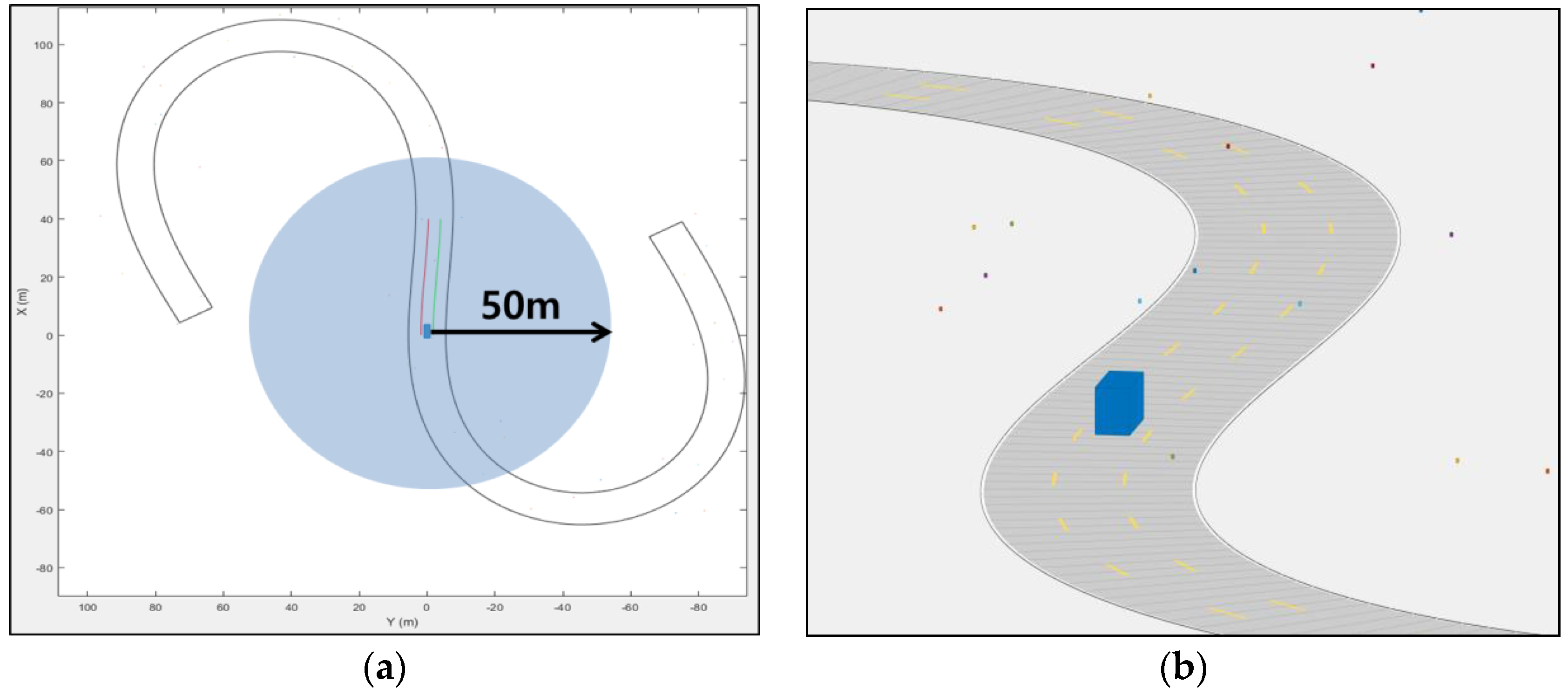
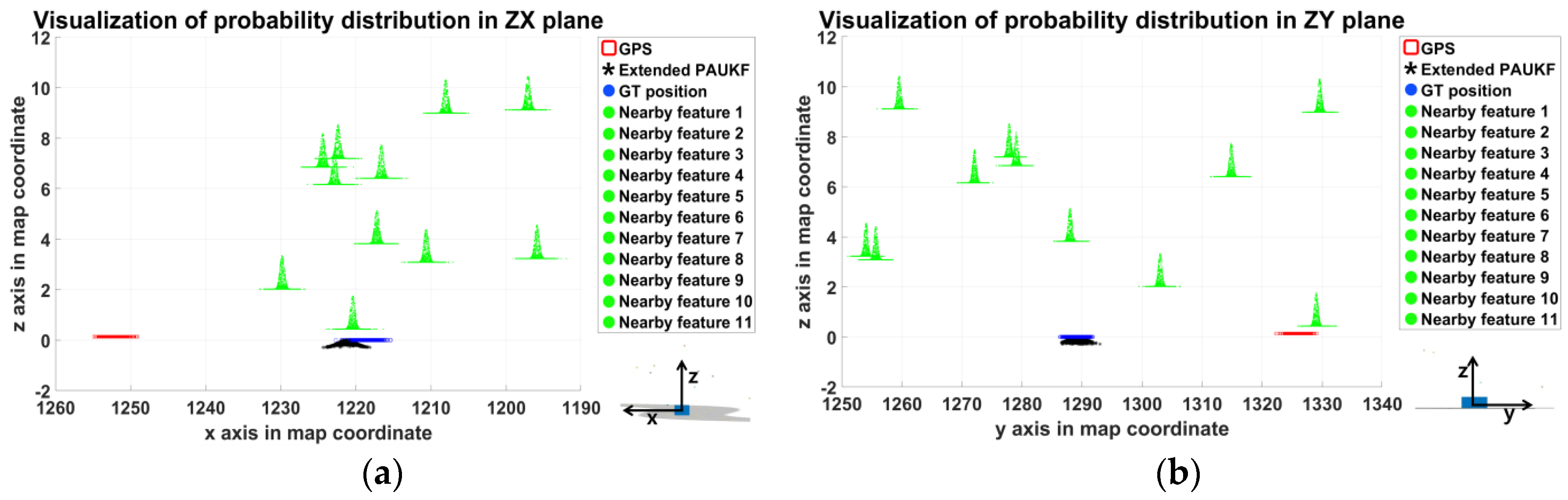
3. Simulation Environment

The simulation environment is based on the MATLAB autonomous driving toolbox. The whole algorithm is made in MATLAB .m file. Since previous research proved no significant differences between S shape roads and straight roads, in this paper, only the S shape road with the 50 m range of perception limit was used, as shown in Figure 3a. The three-dimensional features are generated randomly along the road, as shown in Figure 3b.

The noise setting parameters are shown in

Table 2. Simulation environment setting.

Noise Name	Generate Method
vehicle x-axis error (m)	$~15\sin \left(\mathrm{N}\left(0, 1\right)\right)+\mathrm{N}\left(9.65, 12.2\right)+5)$
vehicle y-axis error (m)	$~15\sin \left(\mathrm{N}\left(0, 1\right)\right)+\mathrm{N}\left(8.34, 12.33\right)+5)$
vehicle z-axis error (m)	$~\mathrm{N}\left(0, 0.09\right)$
$\mathrm{Velocity} \mathrm{error}$ (m/s)	$~\sin \left(\mathrm{N}\left(0, 0.09\right)\right)$
Yaw error (degree)	$~\sin \left(\mathrm{N}\left(0, 0.09 \right)\right)$
Yaw rate error ($\mathrm{degree}/{\mathrm{s}}^2)$	$~\sin \left(\mathrm{N}\left(0, 0.09\right)\right)$
Feature x, y, z error (m)	$~\mathrm{N}\left(0, 0.09\right)$
Feature z position (m)	Random(0,10)
Range sensor bearing error (degree)	$~\mathrm{N}\left(0, 0.09\right)$
Range sensor elevation error (degree)	~$\mathrm{N}\left(0, 0.09\right)$
${\mathsf{\sigma }}_{{\mathrm{PF}}_{\hat{\mathrm{x}}}},{ \mathsf{\sigma }}_{{\mathrm{PF}}_{\hat{\mathrm{y}}}},{ \mathsf{\sigma }}_{{\mathrm{PF}}_{\hat{\mathsf{\theta }}}}$ (m)	5
Random seed	50
Sample time (s)	0.05

. The GPS sensor data is used for the vehicle position initialization and particle initialization. The noise is generated by the normal distribution and transformed with sinusoidal function [29,30]. The onboard noise values are empirical values. The perception error is modeled as a normal distribution in x, y, z-directions. In this paper, we assumed that the perception was performed by a LiDAR sensor. These simulation noise parameters only provide reference results. The perception error depends on the algorithm of the perception module; therefore, it should also be tuned to the actual sensors. The velocity was assumed to be constant. The test velocities of the vehicle were 60 km/h, 70 km/h, 80 km/h, 90 km/h, 100 km/h, 110 km/h, and 120 km/h. The random seed was fixed to 50 for repeatable simulation. The sample time was set as 0.05 s, by considering the perception time. These parameters provide a reference for the performance of the extended PAUKF algorithm. These empirical noise parameters should therefore be tuned with the actual sensor characteristics. We also ran the algorithm in a huge perception error environment to confirm the performance of the algorithm.

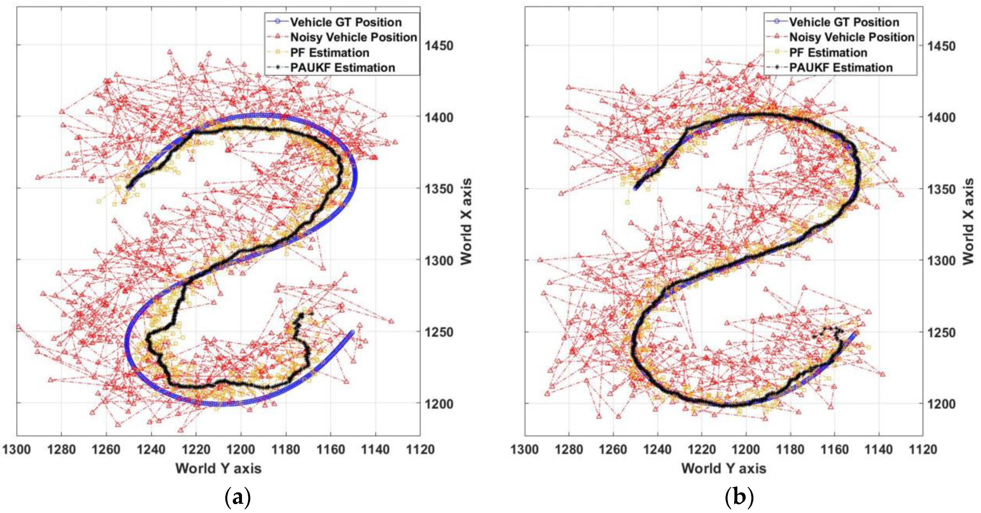
4. Simulation Results

The performance of the previous basic PAUKF and the extended PAUKF were compared based on the root mean square error (RMSE). The performance of filters can be realized by the numerical number of the RMSE of the estimation error. The calculation method of the RMSE of the estimation error is shown as Equation (8).

$$\left[\begin{array}{c}{\mathrm{RMSE}}_{\mathrm{est}}\\ {\mathrm{RMSE}}_{\mathrm{noise}}\end{array}\right]=\left[\begin{array}{c}\sqrt{[{\displaystyle \sum }_{\mathrm{i}=1}^{\mathrm{N}}{\left({\mathrm{Position}}_{{\mathrm{est}}_{\mathrm{i}}}-{\mathrm{Position}}_{{{\mathrm{mean}}_{\mathrm{est}}}_{\mathrm{i}}}\right)}^2]/\mathrm{N}}\\ \sqrt{[{\displaystyle \sum }_{\mathrm{i}=1}^{\mathrm{N}}{\left({\mathrm{Position}}_{{\mathrm{noise}}_{\mathrm{i}}}-{\mathrm{Position}}_{{{\mathrm{mean}}_{\mathrm{noise}}}_{\mathrm{i}}}\right)}^2]/\mathrm{N}}\end{array}\right].$$

(8)

Figure 4a,b show the previous basic PAUKF and the extended PAUKF at 60 km/h, respectively. In both figures, the blue line with the circles is the ground truth trajectory of the vehicle, the red line with the triangles is the noisy vehicle position, the yellow line with the square is the particle filter’s estimation result, and the black line with the circle is the final estimated vehicle position. The estimated trajectory of the previous basic PAUKF showed a significant error in relation to the ground truth trajectory, as shown in Figure 4a, since the previous basic PAUKF did not consider the geometry effect of perception. Furthermore, the previous basic PAUKF did not consider the effect of noise in the vertical direction. As a result, it cannot generate and select appropriately weighted particles. The extended PAUKF by contrast achieved better performance than the previous basic PAUKF, by not only improving the calculation of the geometry, but also by considering the vertical noise effect on the weight generation and the selection scheme. The trajectory of the extended PAUKF was very close to the ground truth data, as shown in Figure 4b.

Figure 5 shows the visualization result of the probability distribution of the features’ position, the ground truth position, the position from the GPS, and the estimated position from the extended PAUKF at 250th sample time. In order to make the figure easy to understand, the origin coordinate of probability distributions translates into the position of features, GPS, and vehicle. One thousand random numbers were used for visualizing the probability of each parameter. In the figure, the red square value is the position from the GPS, the black color with start marker is the position that is estimated from the extended PAUKF, and the blue data with the square is the ground truth data of the vehicle. The figure shows that all the features have different vertical values. The position from the GPS has a large error in relation to the ground truth data. The position from the extended PAUKF estimation is closest to the ground truth data. The extended PAUKF fused the surrounding feature position information to localize the vehicle itself in the map coordinates. This shows the effectiveness of the extended PAUKF.

Table 3. The root mean square error (RMSE) of the basic PAUKF and the extended PAUKF in different conditions (unit: m).

	Position of Vehicle		PF		PAUKF
	Basic	Extended	Basic	Extended	Basic	Extended
60 km/h	30.426	29.465	11.057	6.317	10.199	2.478
70 km/h	30.176	29.351	10.973	6.238	10.314	1.767
80 km/h	29.883	28.319	10.989	6.265	10.458	2.303
90 km/h	29.025	29.919	11.052	5.861	10.627	2.169
100 km/h	29.349	29.981	11.094	6.324	10.893	2.833
110 km/h	28.365	29.144	10.851	6.303	9.751	3.441
120 km/h	29.932	30.072	10.999	6.098	9.826	3.881
Mean	29.571	29.465	11.002	6.201	10.295	2.696
RMSE Change	−0.36%		−43.64%		−73.81%

shows the performance of each filter at a different velocity condition. The velocity of the vehicle was set at intervals of 10, from 60 km/h to 120 km/h. The performance of the filter changed slightly because of random environment effects. The RMSE change of noise shows that the vehicle position noise was almost the same at all velocity conditions. This suggests that both filters were in similar environments. From the RMSE of PF, it can be concluded that the previous basic particle filter estimation’s mean RMSE is 11.002 m and the extended particle filter estimation’s mean RMSE is 6.201 m. The estimation RMSE of PF decreased by about 43.64% compared to the previous PF. The final estimation result is shown in the right column of the PAUKF in Table 3. The mean of RMSE of the previous basic PAUKF was 10.295 m and that of the extended PAUKF was 2.696 m. Compared to the previous basic PAUKF, the extended PAUKF decreased the RMSE by about 73.81%. The extended PAUKF considered the geometry of perception, and improved the weight generation method and selection method. The extended PAUKF may therefore estimate the trajectory precisely.

In order to figure out the performance of the extended PAUKF in a huge perception error environment, we changed the perception noise from $\mathrm{N}\left(0, 0.09\right)$ to $\mathrm{N}\left(3, 9\right)$ in the x, y, z-directions, meaning that the minimum error of relative distance of every feature and vehicle was always larger than 5.196 m. In this noisy environment, with a velocity of 60 km/h, the RMSE of the total RMSE of the extended PAUKF was 5.771 m. Since the measurement variances were not changed, the extended PAUKF still attempted to rely on the measurement from the PF. The algorithm should perform better if we tune the variance of the measurement matrix. This simulation provides a reference for the extended PAUKF in a huge perceived noise environment. The algorithm requires tuning of the hyperparameters before implementation in the real world.

5. Conclusions

In this research, an extended version of particle-aided unscented Kalman filter was proposed for self-driving car localization. The extended PAUKF is based on more realistic assumptions. In this research, we processed the additional uncertainty by expanding the particle’s dimensionality and by improving the weight calculation method of each particle. From the simulation results, we conclude that the previous basic PAUKF has significant limitations in a three-dimensional feature environment. The mean RMSE of estimation based on the previous basic PAUKF was 10.295 m. Compared to the previous basic PAUKF, the extended PAUKF handled the three-dimensional features appropriately. As a result, the mean RMSE of the extended PAUKF was 2.696 m, which represented a 73.81% improvement in precision compared to the previous basic PAUKF, because of the extended particle processing and improved weight selection scheme of the extended PAUKF. We also proposed the feasibility of sensor fusion methodology based on the PAUKF framework. Using our algorithm, a vehicle can receive more precise and robust location information on the basis of traffic lights, road markers, and other traffic elements. However, some limitations still need to be solved. The hyperparameters should be tuned for optimal performance and the motion in vertical direction should be modeled not only by using noise, but also with consideration for the vertical dynamic. In future work, we plan to find the appropriate hyperparameters of the extended PAUKF and implement all the algorithms into a real ground vehicle with consideration for the vertical motion.

References

1. Azmat, M.; Kummer, S.; Moura, L.T.; Gennaro, F.D.; Moser, R. Future Outlook of Highway Operations with Implementation of Innovative Technologies Like AV, CV, IoT and Big Data. Logistics 2019, 3, 15. [Google Scholar] [CrossRef] [Green Version]
2. Jang, S.W.; Ahn, B. Implementation of detection system for drowsy driving prevention using image recognition and IoT. Sustainability 2020, 12, 3037. [Google Scholar] [CrossRef] [Green Version]
3. Wintersberger, S.; Azmat, M.; Kummer, S. Are We Ready to Ride Autonomous Vehicles? A Pilot Study on Austrian Consumers’ Perspective. Logistics 2019, 3, 20. [Google Scholar] [CrossRef] [Green Version]
4. Michail, M.; Konstantinos, M.; Biagio, C.; María, A.R.; Christian, T. Assessing the Impact of Connected and Automated Vehicles. A Freeway Scenario; Springer: Cham, Switzerland, 2017. [Google Scholar]
5. Rose, C.; Jordan, B.; John, A.; David, B. An integrated vehicle navigation system utilizing lane-detection and lateral position estimation systems in difficult environments for GPS. IEEE Trans. Intell. Transp. Syst. 2014, 15, 2615–2629. [Google Scholar] [CrossRef]
6. Kos, T.; Ivan, M.; Josip, P. Effects of multipath reception on GPS positioning performance. In Proceedings of the Elmar—International Symposium Electronics in Marine, Zadar, Croatia, 15–17 September 2010; pp. 399–402. [Google Scholar]
7. Larson, K.M.; Braun, J.J.; Small, E.E.; Zavorotny, V.U.; Gutmann, E.D.; Bilich, A.L. GPS Multipath and Its Relation to Near-Surface Soil Moisture Content. IEEE J. Sel. Top. Appl. Earth Obs. Remote Sens. 2010, 3, 91–99. [Google Scholar] [CrossRef]
8. Meguro, J.I.; Taishi, M.; Jun Ichi, T.; Yoshiharu, A.; Takumi, H. GPS multipath mitigation for urban area using omnidirectional infrared camera. IEEE Trans. Intell. Transp. Syst. 2009, 10, 22–30. [Google Scholar] [CrossRef]
9. Ladetto, Q.; Gabaglio, V.; Merminod, B. Two Different Approaches for Augmented GPS Pedestrian Navigation. In Proceedings of the International Symposium on Location Based Services for Cellular Users (Locellus), Munich, Germany, 5–7 February 2001. [Google Scholar]
10. Yoneda, K.; Chenxi, Y.; Seiichi, M.; Okuya, T.; Kenji, M. Urban Road Localization by using Multiple Layer Map Matching and Line Segment Matching. In Proceedings of the IEEE Intelligent Vehicles Symposium (IV), Seoul, Korea, 28 June–1 July 2015; pp. 525–530. [Google Scholar]
11. Atia, M.M.; Hilal, A.R.; Stellings, C.; Hartwell, E.; Toonstra, J.; Miners, W.B.; Basir, O.A. A Low-Cost Lane-Determination System Using GNSS/IMU Fusion and HMM-Based Multistage Map Matching. IEEE Trans. Intell. Transp. Syst. 2017, 18, 3027–3037. [Google Scholar] [CrossRef]
12. Cong, T.H.; Young Joong, K.; Myo Taeg, L. Hybrid Extended Kalman Filter-based localization with a highly accurate odometry model of a mobile robot. In Proceedings of the 2008 International Conference on Control, Automation and Systems, ICCAS 2008, Seoul, Korea, 14–17 October 2008; pp. 738–743. [Google Scholar]
13. Huang, S.; Gamini, D. Convergence and consistency analysis for extended Kalman filter based SLAM. IEEE Trans. Robot. 2007, 23, 1036–1049. [Google Scholar] [CrossRef]
14. Rezaei, S.; Raja, S. Kalman filter-based integration of DGPS and vehicle sensors for localization. IEEE Trans. Control Syst. Technol. 2007, 15, 1080–1088. [Google Scholar] [CrossRef]
15. Ahmad, H.; Toru, N. Extended Kalman filter-based mobile robot localization with intermittent measurements. Syst. Sci. Control Eng. 2013, 1, 113–126. [Google Scholar] [CrossRef]
16. Lu, J.; Li, C.; Su, W. Extended Kalman filter based localization for a mobile robot team. In Proceedings of the 28th Chinese Control and Decision Conference, CCDC 2016, Yinchuan, China, 28–30 May 2016; pp. 939–944. [Google Scholar]
17. Faisal, M.; Ramdane, H.; Mansour, A.; Khalid, A.-M.; Hassan, M. Robot localization using extended kalman filter with infrared sensor. In Proceedings of the IEEE/ACS International Conference on Computer Systems and Applications, AICCSA, Doha, Qatar, 10–13 November 2014; Volume 2014, pp. 356–360. [Google Scholar]
18. St-Pierre, M.; Denis, G. Comparison between the unscented Kalman filter and the extended Kalman filter for the position estimation module of an integrated navigation information system. In Proceedings of the IEEE Intelligent Vehicles Symposium, Parma, Italy, 14–17 June 2004; pp. 831–835. [Google Scholar]
19. Ndjeng, A.N.; Alain, L.; Dominique, G.; Sébastien, G. Experimental comparison of kalman filters for vehicle localization. In Proceedings of the IEEE Intelligent Vehicles Symposium, Xi’an, China, 3–5 June 2009; pp. 441–446. [Google Scholar]
20. Zhu, H.; Huosheng, H.; Weihua, G. Adaptive unscented Kalman filter for deep-sea tracked vehicle localization. In Proceedings of the 2009 IEEE International Conference on Information and Automation, ICIA 2009, Zhuhai/Macau, China, 22–24 June 2009; pp. 1056–1061. [Google Scholar]
21. Tamimi, H.; Henrik, A.; André, T.; Tom, D.; Andreas, Z. Localization of mobile robots with omnidirectional vision using Particle Filter and iterative SIFT. Robot. Auton. Syst. 2006, 54, 758–765. [Google Scholar] [CrossRef] [Green Version]
22. González, J.; Blanco, J.-L.; Cipriano, G.; Ortiz-de-Galisteo, A.; Juan-Antonio, F.-M.; Francisco Angel, M.; Jorge L, M. Mobile robot localization based on Ultra-Wide-Band ranging: A particle filter approach. Robot. Auton. Syst. 2009, 57, 496–507. [Google Scholar] [CrossRef]
23. Vlassis, N.; Terwijn, B.; Ben, K. Auxiliary particle filter robot localization from high-dimensional sensor observations. In Proceedings of the IEEE International Conference on Robotics and Automation, Washington, DC, USA, 11–15 May 2002; Volume 1, pp. 7–12. [Google Scholar]
24. Martin, A.; Sen, Z.; Lihua, X. Particle filter based outdoor robot localization using natural features extracted from laser scanners. In Proceedings of the IEEE International Conference on Robotics and Automation, New Orleans, LA, USA, 26 April–1 May 2004; Volume 2, pp. 1493–1498. [Google Scholar]
25. Montemerlo, M.; Sebastian, T.; William, W. Conditional Particle Filters for Simultaneous Mobile Robot Localization and People-Tracking. In Proceedings of the IEEE International Conference on Robotics &Automation, Washington, DC, USA, 11–15 May 2002; pp. 695–701. [Google Scholar]
26. Lin, M.; Yoon, J.; Kim, B. Self-driving car location estimation based on a particle-aided unscented Kalman filter. Sensors 2020, 20, 2544. [Google Scholar] [CrossRef] [PubMed]
27. Thrun, S.; Burgard, W.; Fox, D. Probabilistic Robotics; MIT Press: Cambridge, UK, 2000. [Google Scholar]
28. Ristic, B.; Sanjeev, A.; Neil, G. Beyond the Kalman Filter; Artech House: London, UK; Norwood, MA, USA, 2003. [Google Scholar]
29. Minfen, S.; Francis, H.Y.C.; Patch, J.B. A method for generating non-Gaussian noise series with specified probability distribution and power spectrum. In Proceedings of the IEEE International Symposium on Circuits and Systems, Bangkok, Thailand, 25–28 May 2003; Volume 2. [Google Scholar]
30. Suhr, J.K.; Jang, J.; Min, D.; Jung, H.G. Sensor Fusion-Based Low-Cost Vehicle Localization System for Complex Urban Environments. IEEE Trans. Intell. Transp. Syst. 2017, 18, 1078–1086. [Google Scholar] [CrossRef]
Figure 1. Vehicle state of the particle filter.
Applsci 10 05045 g001
Figure 2. The effect of three-dimensional perception.
Applsci 10 05045 g002
Figure 3. (a) Maximum perception range; (b) randomly generated 3D feature along the road.
Applsci 10 05045 g003
Figure 4. (a) Position estimation result of the basic particle-aided unscented Kalman filter (PAUKF) at 60 km/h; (b) position estimation result of the extended PAUKF at 60 km/h.
Applsci 10 05045 g004
Figure 5. The probability distribution at 250th sample time. (a) Visualization of the probability of values at ZX plane; (b) visualization of the probability of values at ZY plane.
Applsci 10 05045 g005