Article

Quantum Dilation and Erosion

1
Department of Physics, College of Arts and Sciences, Cornell University, New York, NY 14853, USA
2
Department of Physics, University of Science and Technology of China, Hefei 230026, Anhui, China
3
College of Engineering, Abu Dhabi University, Abu Dhabi 59911, UAE
4
Software Engineering Department, Lakehead University, Thunder bay, Ontario, ON P7B 5E1, Canada
5
College of Arts and Sciences, Abu Dhabi University, Abu Dhabi 59911, UAE
6
Institute for Quantum Science and Engineering, Texas A&M University, College Station, TX 77843, USA
*
Author to whom correspondence should be addressed.
Appl. Sci. 2020, 10(11), 4040; https://doi.org/10.3390/app10114040
Submission received: 29 April 2020 / Revised: 1 June 2020 / Accepted: 4 June 2020 / Published: 11 June 2020
(This article belongs to the Section Quantum Science and Technology)

Abstract

:
The dilation and erosion operations are the first fundamental step in classical image processing. They are important in many image processing algorithms to extract basic image features, such as geometric shapes; such shapes are then fed to higher level algorithms for object identification and recognition. In this paper, we present an improved quantum method to realize dilation and erosion in imaging processing. Unlike in the classical way, in the quantum version of imaging processing, all of the information is stored in quantum bits (qubits). We use qubits to code the location and other information of each pixel of the images and apply quantum operators (or quantum gates) to accomplish specific functions. Because of quantum entanglement and other nonintuitive features in quantum mechanics, qubits have many advantages over classical bits, but their nature presents challenges in designing quantum algorithms. We first built the quantum circuit theoretically, and then ran it on the IBM Quantum Experience platform to test and process real images. With this algorithm, we are looking forward to more potential applications in quantum computation.

1. Introduction

Image analysis is a technique of extracting useful information from images [1,2] using various computer vision algorithms. Image processing has been on the rise for many years [3]. The concept of image analysis is applicable in multiple fields like health, technology, government sectors, etc. The main objective of image processing is to analyze and capture the features of an image like its size, shape and various other characteristics. It has majorly impacted the health industry by enabling quicker analysis of blood cells to identify various diseases [4]. This technique is also being used by governments to work towards road safety by using computer vision algorithms in radars to capture the digits of vehicle number plates [5]. Morphological image processing is a crucial component of image processing relating to shape or morphology features of the image [6]. Structuring element is a central element of image morphology, in the form of a matrix of binary pixels. The structuring element either fits or intersects the image based on the binary value of the pixels, and it is applied to the input image to generate an output image. Dilation and erosion [2], in simpler terms, opening and closing, are the two eminent morphological operators [7]. These operators are used for a variety of tasks like eradicating noise, detecting outliers in the image, i.e., its depressions, holes etc. as well as linking and separating various elements in the image. Erosion is done to remove details in a binary image which results in reducing the size of the image, whereas dilation enlarges the image by connecting the gaps within the image pixels. Dilation and erosion act opposite to each other when applied on a binary image, with the structural element being the deciding factor in the outcome of the image.
Quantum morphology operations [8] are propounded based on the novel enhanced quantum representation model. The quantum logical operators are the base on which the quantum morphology operations are implemented. These quantum logical operators perform operations on pixels based on their corresponding pixel value within dual or multiple images. Logic gates are employed to transform input qubits to the same number of output qubits depending on the computation of the gates. Here, we will look at two quantum gates, the Toffoli gate and Swap gate. The Toffoli gate, aka CCNOT (controlled-controlled-not) gate [9,10], is a reversible logic gate which inverses the output bits based on the input bits. The swap gate interchanges the qubits based on their placement in the matrices.
In the paper written by Yuan et al. [11], a very interesting algorithm is proposed. They make use of the quantum circuits to accomplish the functions of dilation and erosion. Compared with the classical dilation and erosion algorithms, which are fundamental in classical image processing, this algorithm is pure quantum; that is, all of the operations are realized by the quantum gates in a quantum circuit. Although dilation and erosion are not very complicated algorithms, they require many of the conditions we need in quantum image processing. In this algorithm, a system for using qubits to code and process image information is built, so it could be easily applied to other algorithms in quantum image processing. The idea for the algorithm could also be applied into many other fields. This is a very practical attempt, or a good start, to the future use of real computers, which scientists all over the world are working on. This fundamental application promises the transplant action of more algorithms into quantum circuits in the future.
However, the proposed algorithm is not completely accurate due to the ambiguous definition of the qubits for different information in the images, which we will discuss in this paper. Here, we propose a more consistent algorithm for quantum dilation and erosion as well as its implementation in the IBM quantum simulator.

2. Preliminaries

In this section we give a brief review of the basic theories on state vector and the quantum representation of images [12,13,14].

2.1. Quantum Representation

In quantum computation, a system is represented by a vector in a Hilbert space. The vector is denoted by a Dirac notation | u . The smallest unit of information in the vector (i.e., the quantum system) is called a qubit which can be described as follows:
| φ = α | 0 + β | 1 = α 1 0 + β 0 1 ,
where α and β represent complex numbers satisfying | α | 2 + | β | 2 = 1 . The notation of | k in n qubit system means | k n 1 k 1 k 0 , where k n 1 k 1 k 0 designs the binary representation of k in n digits.

2.2. Morphological Image Processing

Morphological operators are a well established set of image processing operations often used to extracting geometric features from binary and gray scale images.
In image processing literature basic geometric shapes (such as circle, triangles, etc.) are detected by applying certain image operators; the output depends on whether or not the geometric shape is present inside the given image.
Clearly, the image operators to detect certain geometric features depend on the shape and size of the feature to be extracted.
Morphological Set operators such as union, intersection, inclusion, and complement can be directly generalized to gray-scale images of any dimension by considering the point-wise maximum and minimum operators.
The shape detection process starts by developing a structure element (SE) which is a small binary matrix with patterns of zeros and ones that represent the shape of interest. For example, to detect circles in an image, the structure element can be defined as a matrix with all ones on the perimeter of the circle and zero otherwise.

2.3. Operators in Set Theory

In image processing literature, the mathematical morphological operators are composed of few simple mathematical concepts from set theory.
In set theory, the fundamental set operators are the intersection ∩ and the union ∪ operators.
For binary image, they are denoted by
C = A B , D = A B .
For gray level images, the union operator is defined as the point-wise maximum operator ∨ and the intersection operator is defined as the point-wise minimum operator ∧,
( f h ) ( x ) = m a x [ f ( x ) , h ( x ) ] , ( f h ) ( x ) = m i n [ f ( x ) , h ( x ) ] .
The translation of set S by point z = ( z 1 , z 2 ) , connoted ( S ) z , is defined as
( S ) z = { c | c = s + z , s S } .

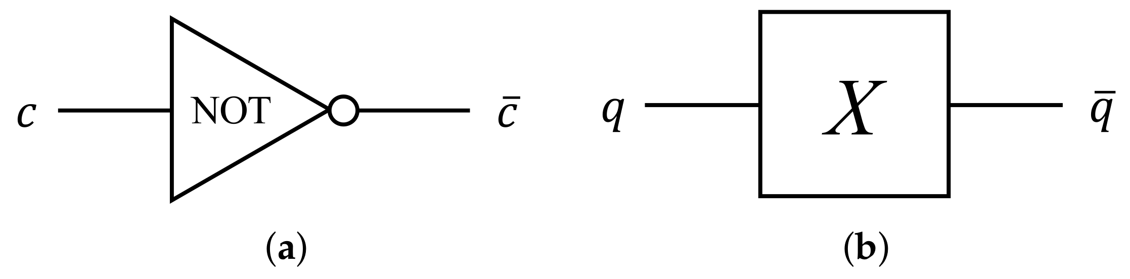
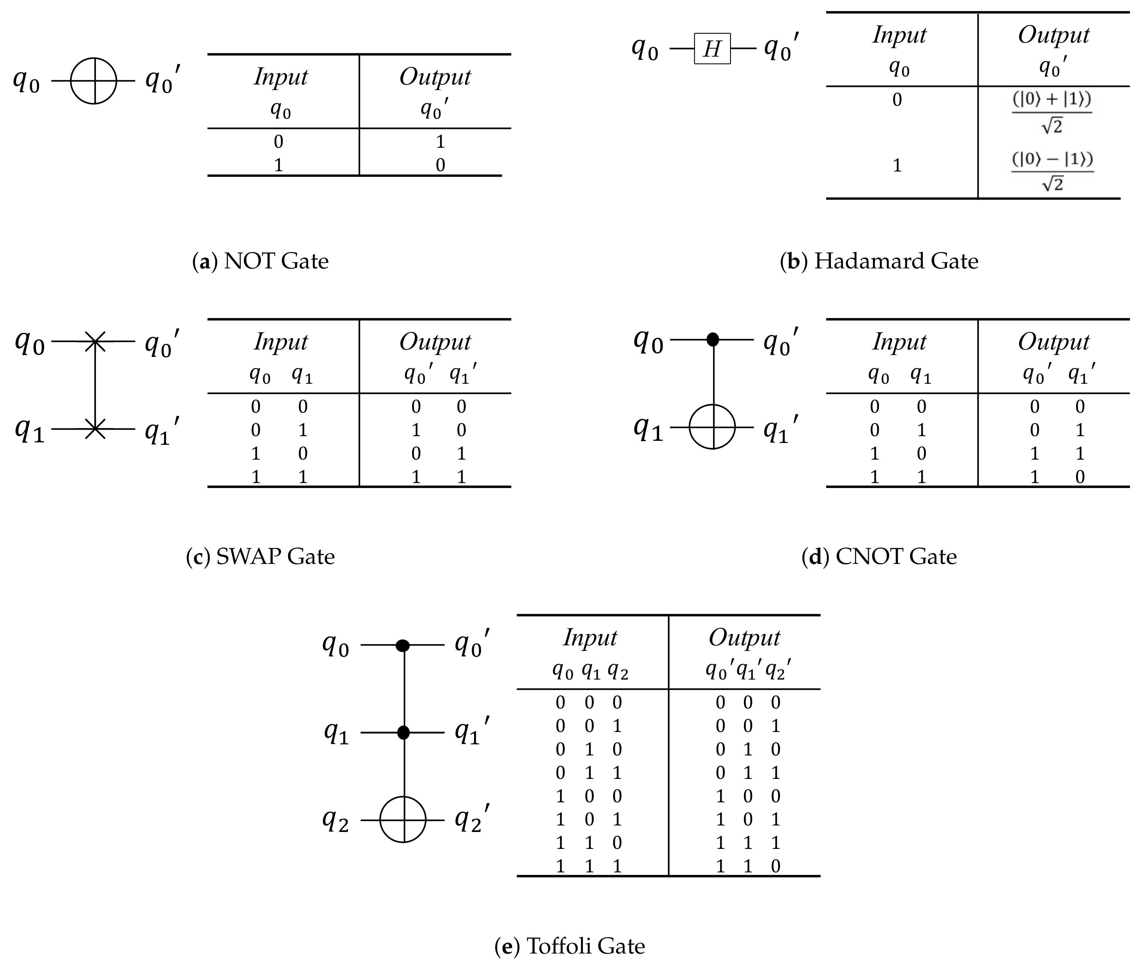
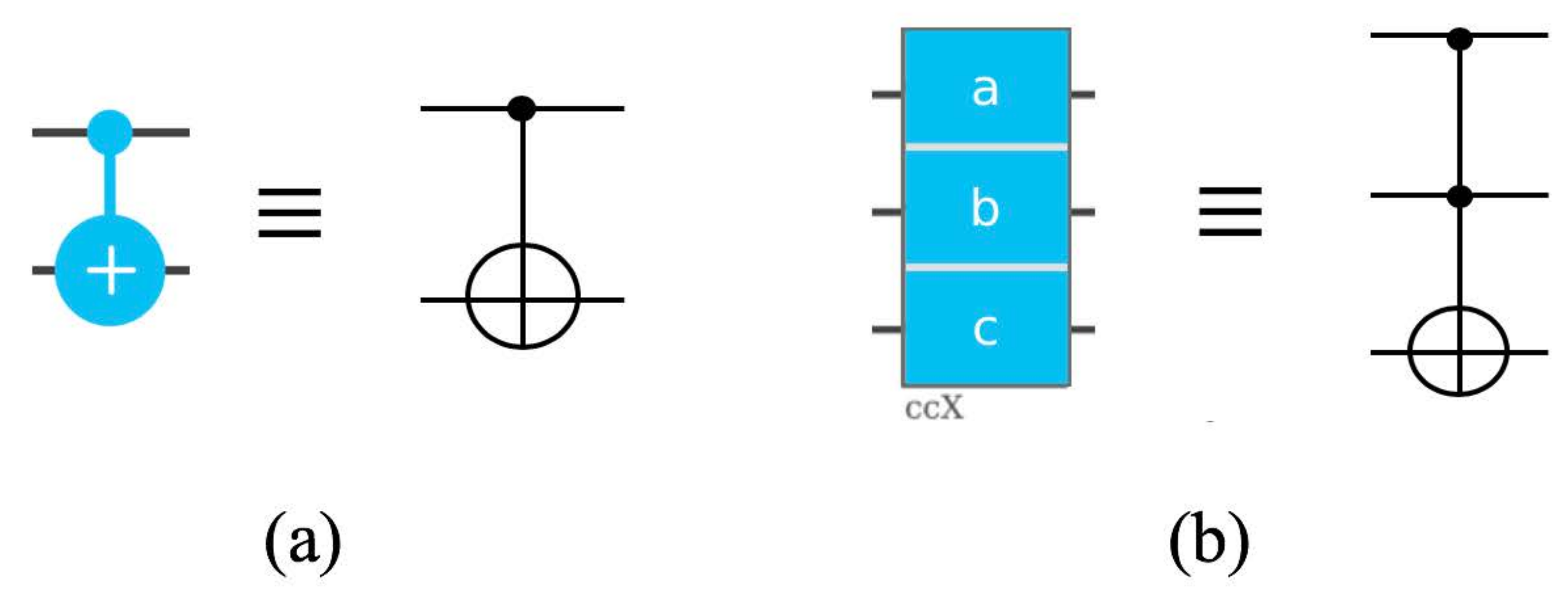
2.4. Operators in Quantum Circuits

The quantum circuit is composed of “wires” and “gates”. Wires are represented by the qubits that store information, while gates are utilized to execute computational operations. In some sense, the quantum circuit presents some similarity to the classical circuit such as, the classical NOT gate (Figure 1a) and the quantum NOT gate (X gate, Figure 1b). They act in the same way as flipping the state of a bit/qubit.
Classical binary gates are irreversible and the input logic state cannot be uniquely inferred from the output. For example if the output of the logic AND gate is logic 0, the input could be one of three states (00, 01 or 10). On the other hand all the gates in quantum circuits are reversible. NOT gate is considered as the central operation in both classical and quantum gate circuits. However, NOT gate is defined for only a one-qubit operation, it is not adapted for interactions between different qubits. By adding a control qubit to the NOT gate, we get the “controlled-NOT” gate, or CNOT gate. If the control qubit is | 0 , the target qubit will not be changed. For the control qubit with value | 1 , the target qubit is flipped. See Figure 2d for the representations and table truth of the CNot-gate. The function of CNOT gate can be represented also as | q 0 , q 1 | q 0 , q 0 q 1 where q 1 represents the control qubit, and ⊕ refers to the operation plus modulo 2. By adding another control qubit to the CNOT gate, we realize the “controlled-controlled-NOT” gate, which is also known as “Toffoli gate”. The target qubit is flipped only if both control qubits have the value | 1 . This gate is also represented by | q 0 , q 1 , q 2 | q 0 , q 1 , q 2 q 0 q 1 , where q 0 , q 1 design the control qubits [10] (Figure 2e).
Toffoli gate is considered as a universal reversible classical gate [15,16]. A universal gate is defined as a building block from which all other gates can be constructed. Nevertheless, toffoli gate is not enough to built a universal quantum gate, we need to combine with the single qubit Hadamard gate in order to obtain the universal quantum gate. We realize quantum circuit by using multiple gates in order to simplify the implementation.

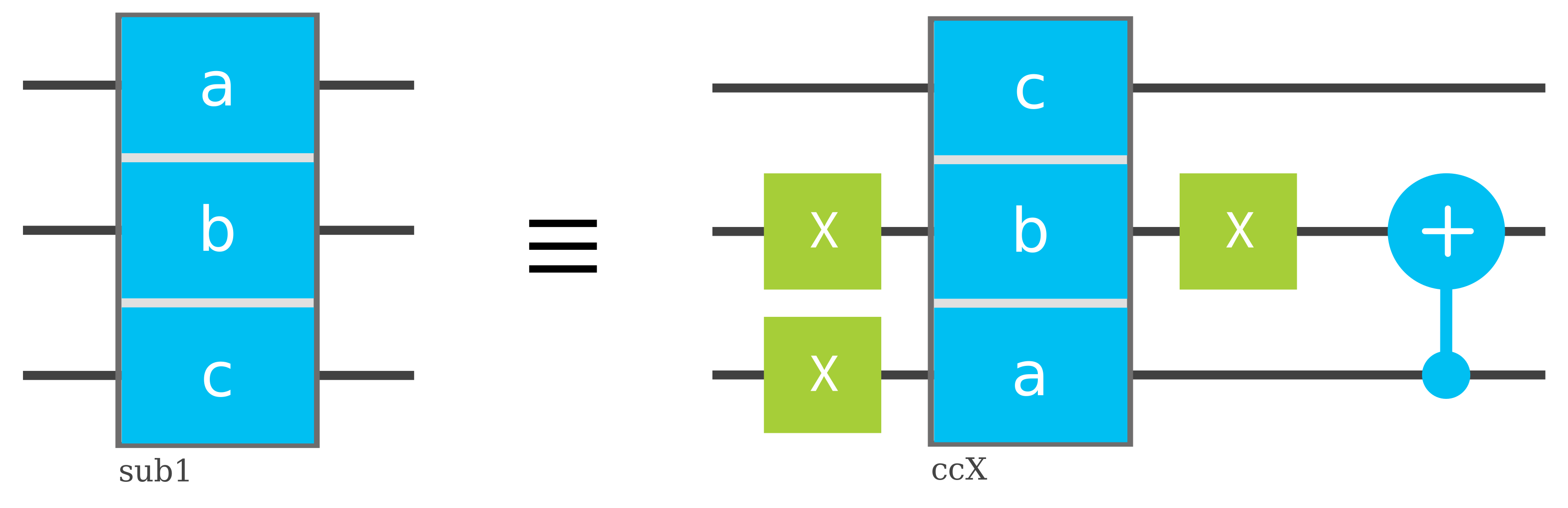
3. Quantum Dilation and Erosion Operations

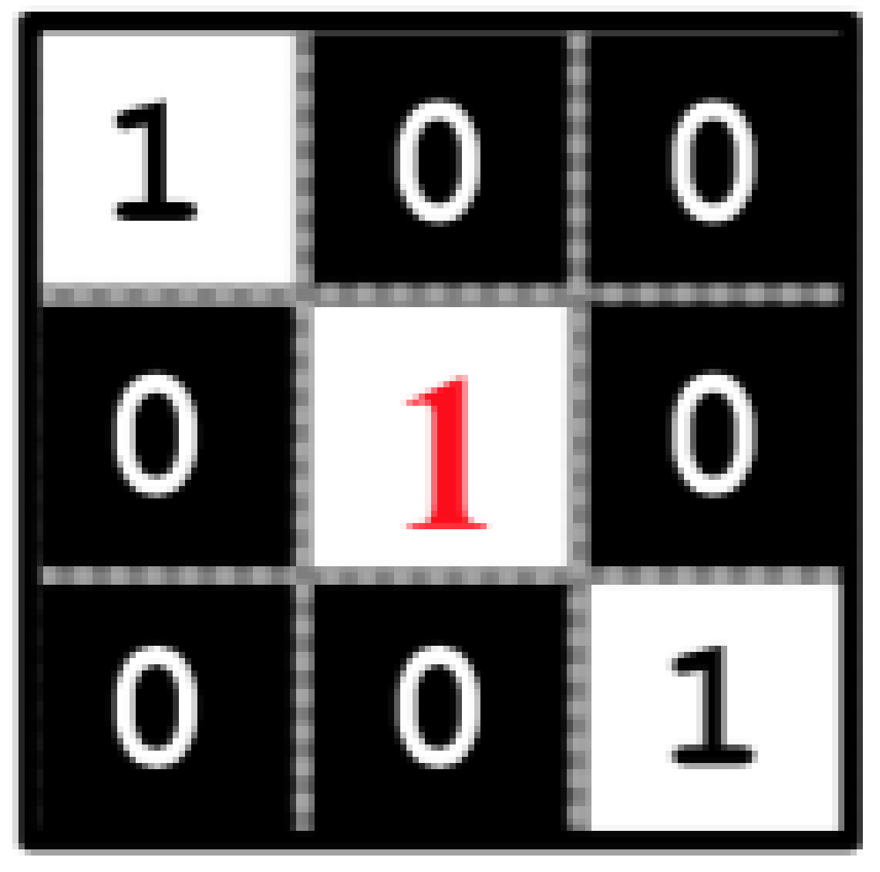
3.1. Image Representation

In black and white images, referred as binary images, the gray has the value either 0 or 1. The expression representing the 2 n × 2 n binary image is given by [17]:
| I = 1 2 n Y = 0 2 n 1 X = 0 2 n 1 | G Y X | Y X ,
where | G Y X encrypts the binary information, and | Y X defines the position information.

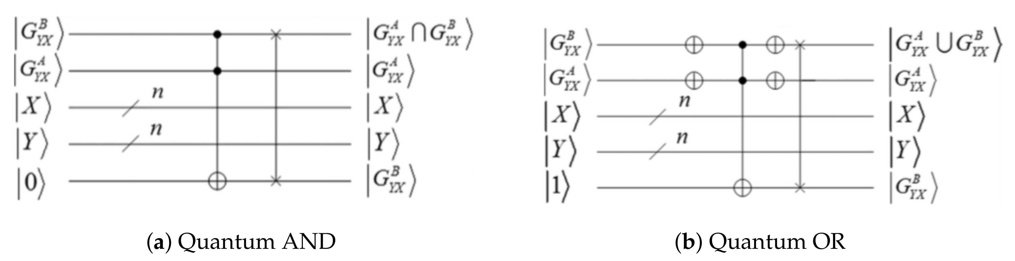
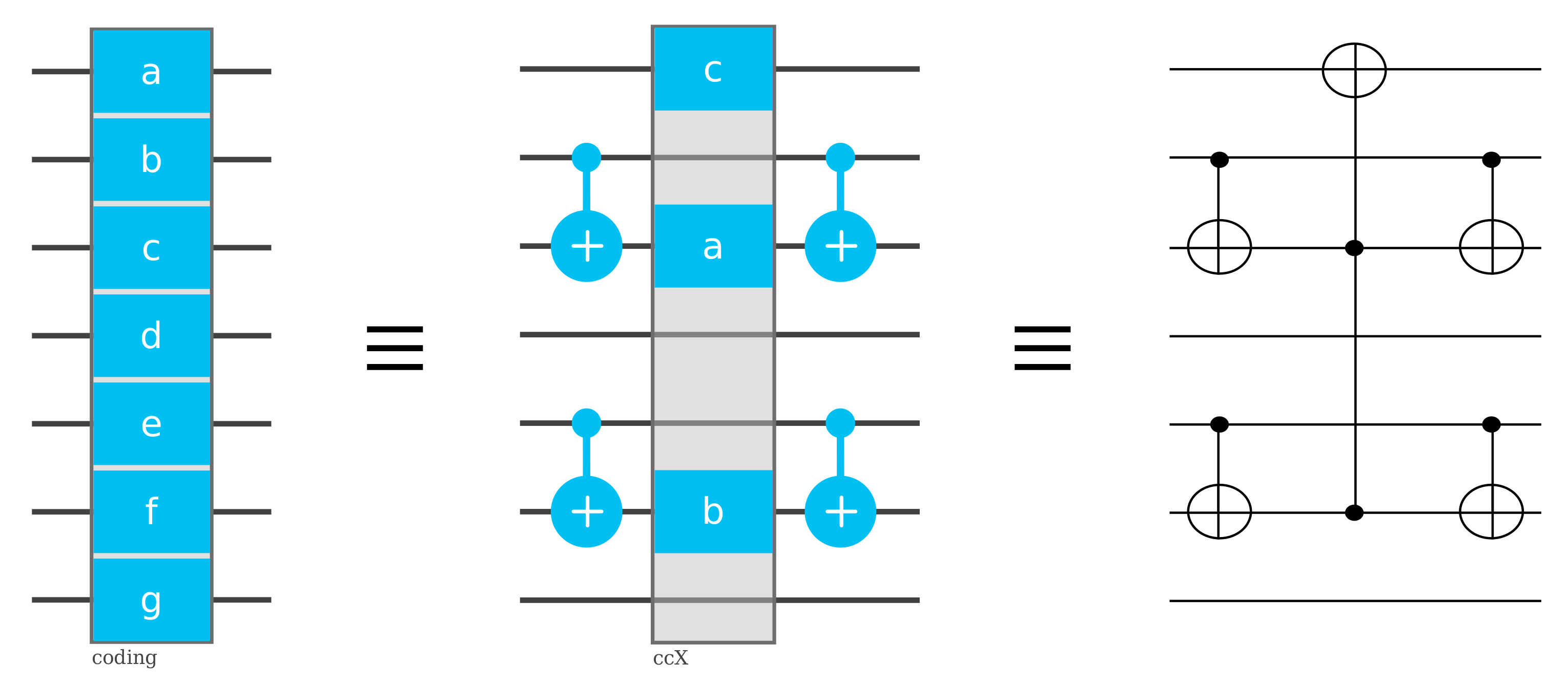
3.2. Quantum Logical Operations

Quantum AND and OR gates can be identified by the notations ∩ and ∪, respectively. The AND operation can be accomplished by Toffoli gate, that is, when both of the control qubits are | 1 , the target will be flipped. When we use an ancillary qubit initialized as | 0 as the target qubit and the control qubits for the two input states (representing two binary images A and B with the size 2 n × 2 n ) | G Y X A and | G Y X B , we can obtain the result of AND gate operation | G Y X A G Y X B after the SWAP gate in the target qubit. Figure 3a presents the quantum circuit of AND operation. Similarly, according to the symmetry of AND and OR operation, we can obtain the circuit for OR gate operation by Toffoli gate with NOT gate (Figure 3b).

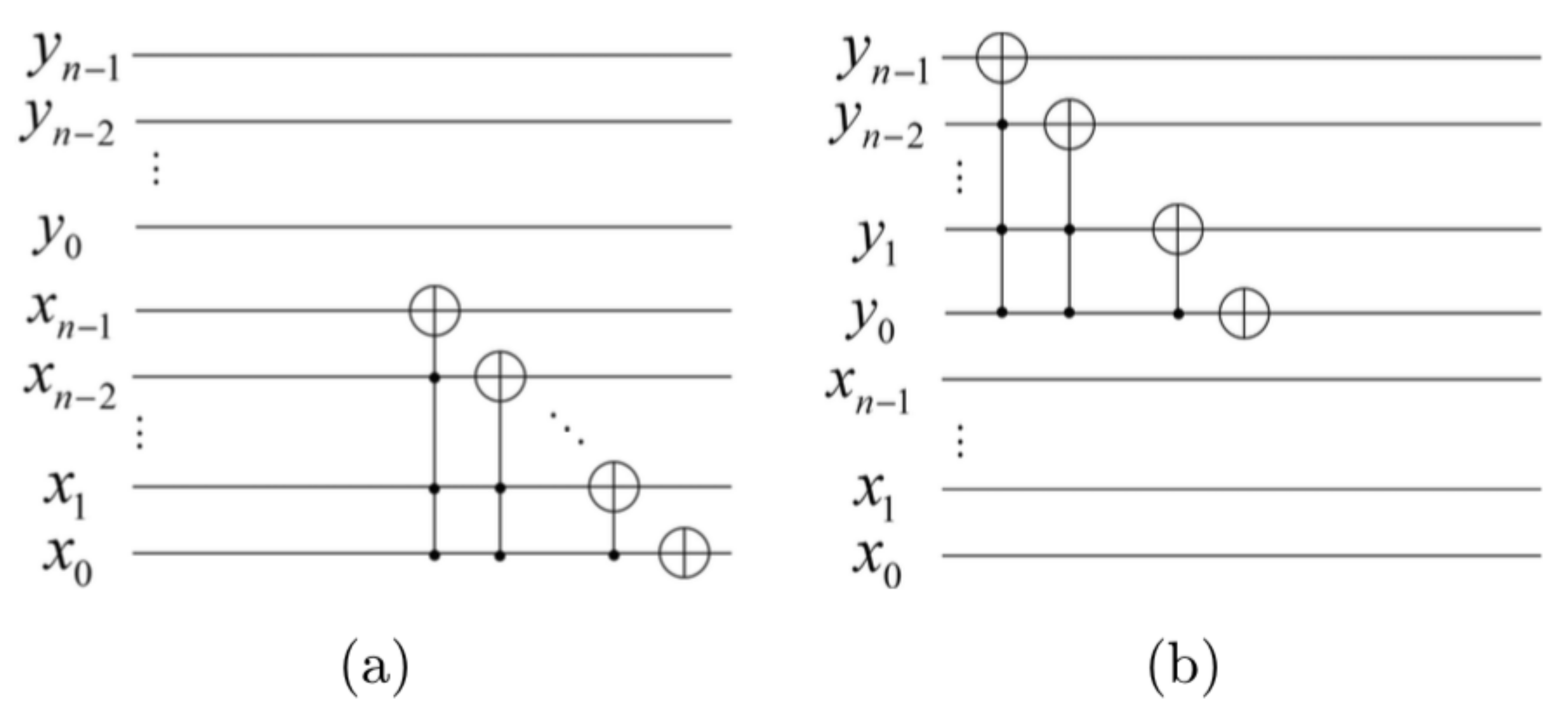
3.3. Position Shifting Transformation

In order to shift the whole image, here we introduce the position shifting transformation (Figure 4).
We can see the “add one” operation for a binary number is to flip the last “0” and all the following serial “1”s; the circuit perfectly accomplishes this function. In addition, when the number exceeds the maximum 2 n 1 , it will return to 0 automatically, so this operation is good for image shifting. If we swap all of the 0s and 1s the addition is changed to subtraction. Thus we can accomplish the “subtract one” operation in a similar way. Since all of the positions are changed, the stored image would shift as a whole. By applying the “add one” and “subtract one” operations, one can easily shift the image to any position. It is an essential operation in both dilation and erosion.

3.4. Dilation and Erosion

The pertinent structures of the image are extract by dilation and erosion which are considered as morphological operators. This can be accomplished by probing the image with another set of given shape—the structuring element (SE). The Dilation operation is defined as following: let us take the structure element S as a mask. The reference point of the structure element is placed on all pixels in the image that have the value 1 in A S . It is worth mentioning that this process is similar to convolution or cross-correlation of the image A with the mask S. Here for every position of the mask, instead of forming a weighted sum of products, we place the elements of S into the output image.
So, the dilation “thickens” or “grows” objects in the binary image.
In contrast, erosion “shrinks” or “thins” objects in the binary image. consequently, we can conceive the erosion operation as opposite to dilation.
The erosion of A by S, connoted by A S , is defined as: the output image A S is set to zero. S is placed at every masked point in A. If A contains S (for non-zero A AND S) then S is placed in the output image. The output image is the set of all elements for which S, translated to every point in A, is contained in A.

3.5. Operations

Let us consider a 2 n × 2 n binary image A, and a ( 2 k + 1 ) × ( 2 k + 1 ) structure element S. Their origin is located in the center point. The quantum dilation of A by S, denoted by A S is defined as
A S = { z | ( S ) z A } , z = | Y X ,
where
( S ) z = { c | c = s + z , s S } .
The quantum erosion of A by S, denoted by A S , is defined as
A S = { z | ( S ) z A c = } , z = | Y X ,
where A c is the complement of A.

3.6. Yuan’s Algorithm Problem

Yuan et al. [11], proposed an “improved quantum binary dilation operation” which requires replications of the quantum image state | I Y X . However, in their demonstration, they replicated the grey scale (color) qubits ( | Y X ) as well as the location qubits( | G ).
Therefore, given different copies of the image states, multiple copies of the location states | Y X were obtained as well, leading to the loss of the quantum correlations of the different images, i.e., all of the images are actually independent of each other. When we apply the operations to the replicated images, we do not obtain useful results.
We can see this from Figure 3. We can use the quantum AND and OR operations because the two images, A and B, share the same location states | Y X . In this way, they are correlated so that we can produce the right outcome of using quantum AND and OR. Yuan’s algorithm uses multiple images with different locations which can not be realized by the quantum AND and OR operations as the authors stated. Let us consider for simplicity two images, | I Y X A and | I Y X B , with two different location states, | Y X A and | Y X B , the procedure demonstrated in Figure 3 can not be done, since there is no quantum correlation.
In the following section, we discuss how we fix this problem and thereby improve the procedure of the “improved quantum binary dilation operation”.

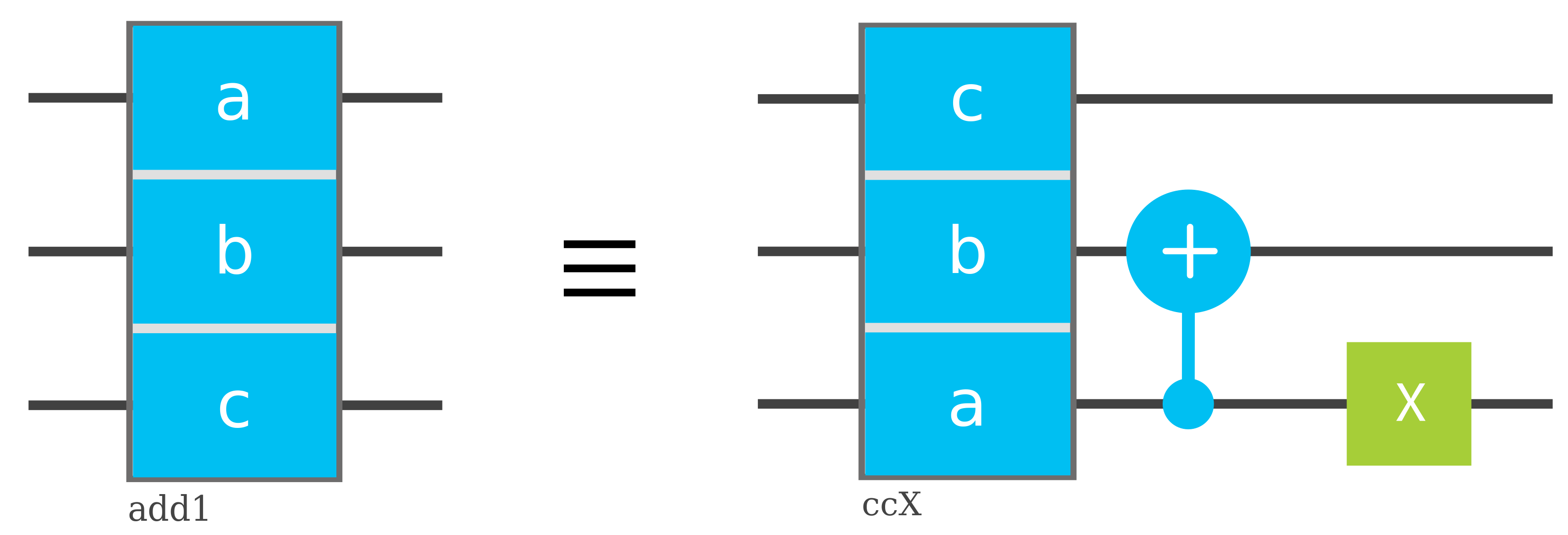
3.7. Our New Implement Procedure

Generally, suppose that the size of S is ( 2 k + 1 ) × ( 2 k + 1 ) , and then the structuring element S can be written in the form of matrix w as
w = h Y k , X k h Y k , X + k h Y , X h Y + k , X k h Y + k , X + k ,
where h i , j is either 0 or 1. Then, the quantum binary dilation of A by S can be obtained from the following steps:
Step 1: Prepare the location state | Y X and h qubits for color information | G Y X of the same quantum image | I Y X . These h qubits of | G Y X can be written as
{ | G Y X 1 , | G Y X 2 , , | G Y X h } ,
and the value of h is given by
h = h Y k , X k + h Y k , X k + 1 + + h Y , X + + h Y + k , X + k ,
where h i , j { 0 , 1 } .
Step 2: Code the image information to the h qubits of | G Y X . The position shifting transformation is applied to shift the image, then we obtain the set as
{ h Y k , X k | G Y k , X k , , h Y X | G Y X , , h Y + k , X + k | G Y + k , X + k } ,
where h i , j { 0 , 1 } . When h i , j = 0 , it means that | G i j is not needed. When h i , j = 1 , we need to obtain quantum state | G i j by performing the proper position shifting operation on the quantum state | G Y X obtained in step 1.
Note that all the images share the same location states | Y X , so after coding we need to apply another inverse position shifting transformation to restore the original | Y X . Then we have the h | G states.
Step 3. Obtain the improved quantum binary dilation and erosion operations. We need another qubit(s) | O to store the result of the new information.
For dilation, we apply the quantum OR operation, | O = h | G ; for erosion, we apply the quantum AND operation, | O = h | G . By measuring the output | O as well as the location states | Y X , we can obtain the results of the quantum dilation or erosion.

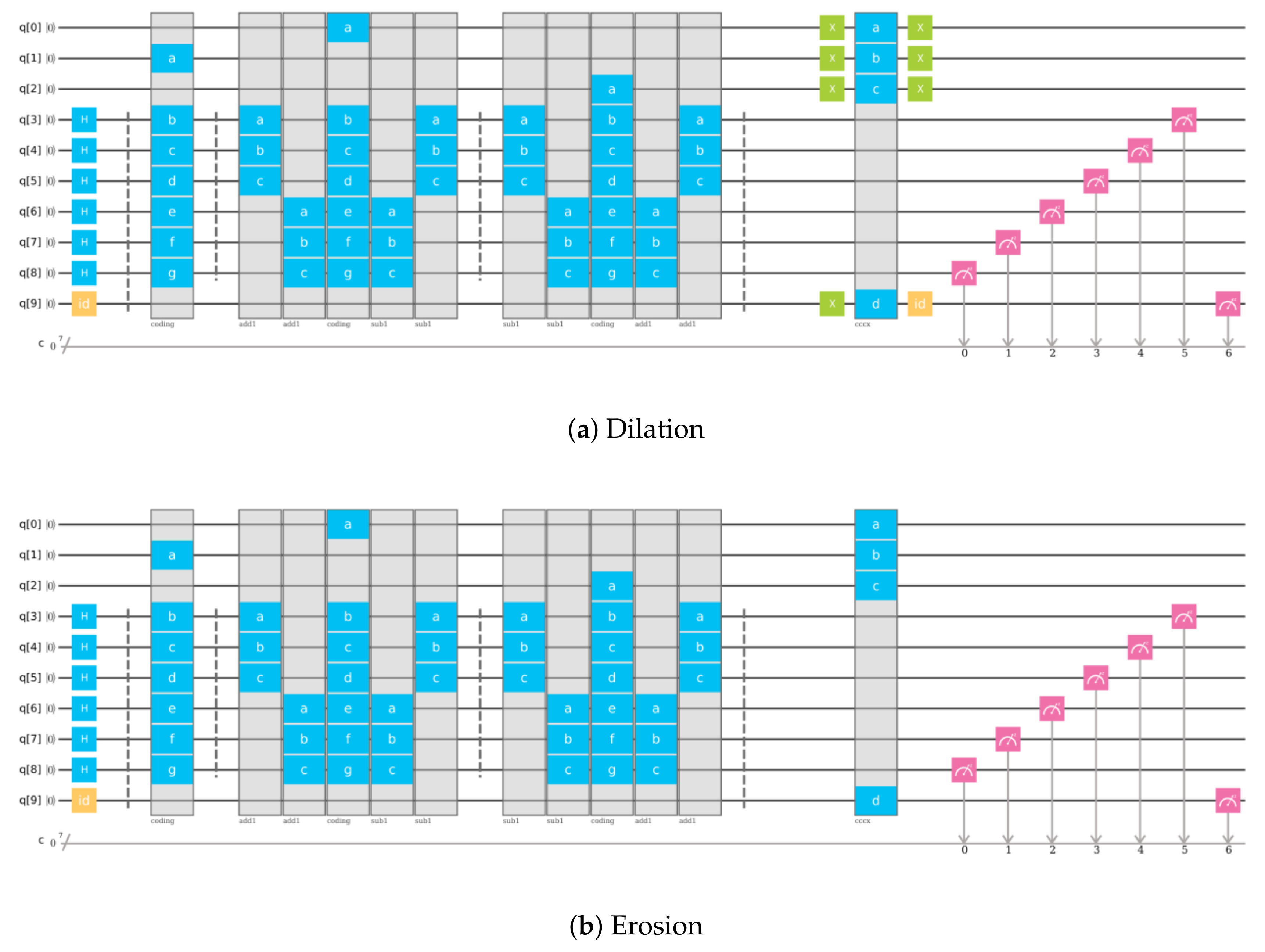
4. Implementation on IBM QE

4.1. The “Quantum Score” on IBM QE

IBM Quantum Experience was used to implement our quantum circuit. This quantum computer has its own symbols for the quantum gates. The blue stick with a big and a small circle on both sides is the CNOT gate (shown in Figure 5a). Just like the general notation of CNOT gate, the bigger circle with a plus sign is the target qubit, while the smaller circle denotes the control qubit. To measure the value of the qubits. In this way, we can read out the results of every qubit in the quantum circuit.
Besides some basic gates, this platform also provides a function for users to write their own self-designed gates. By this function one can make the quantum circuit more concise. A series of simple quantum gates can be integrated as a single self-designed gate, so that we can use only one gate to indicate the whole subroutine. For example, the “ccX” gate (controlled-controller-X gate, or the Toffoli gate), as shown in Figure 5b, can be represented by the blue box with the distinguished qubits denoted by the letters “a”, “b” and “c”. In the following sections there are more examples about this subroutine representation.

4.2. Image Coding

Here we give examples to show every detail of implementation. Suppose an image of 8 × 8 = 64 pixels, which means we need three qubits for Y and three qubits for X, in total six qubits for the location states. To simplify the system, we only use one qubit for the color information | G .
Suppose an image that has a white square of 4 × 4 pixels in the middle, and rest of the image is black. We denote black as | 0 and white as | 1 for | G , we can obtain the state of the image as
| I = 1 2 n Y = 0 2 n 1 X = 0 2 n 1 | G Y X | Y | X .
In order to accomplish this image state, it is easy to find that the circuit in Figure 6 can construct the state | I from the initial state | I 0 = 1 2 n Y = 0 2 n 1 | Y X = 0 2 n 1 | X .
The “coding” subroutine in Figure 6 accomplishes the target image state from the initial state with all | 0 s. Letters in the blue blocks denote the different qubits in this multi-qubit operation, where a is the qubit for color information, | G ; the position qubits | Y and | X consist of bcd and efg. The diagram in the middle of Figure 6 shows the composition in quantum IBM Q experience. Its counterpart is represented in quantum circuit notation on the right. This coding process including four CNOT gates and one Toffoli gate (“ccX”). By the first two CNOT gates, one can find that only the states after | 0 in Equation (13) can cause the target qubit to be flipped, so that the | G is coded. For example, if | Y = | 101 and | X = | 010 (i.e., bcd = 101 and efg = 010), the target qubit c of the upper CNOT is flipped from | 0 to | 1 because its control qubit b = | 1 , and for the lower CNOT, the target qubit f remains the input value | 1 as the control qubit e = | 0 . While qubit c and f are the control qubits of the following Toffoli (“ccX”) gate, the target qubit of the gate, which is qubit a, will be flipped because both qubit c and f are | 1 in this case. We put the other two CNOT gates at last just to counteract the influence from the previous CNOT gates, so that after the whole subroutine the states of qubit c and f will remain the same (if they are flipped by the first CNOT, they will be flipped back). In this way, the coding subroutine only encodes the color information qubit a while remains the position qubits unchanged.

4.3. Structure Element and Position Shifting

After the original image, we have a structure element shown in Figure 7. In this structure element we can see the number of ones h = 3 , so we need three | G s for the image information with different position shifting. The set of the image information states is
[ H ] | G Y 1 , X 1 , | G Y , X , | G Y + 1 , X + 1 .
Regarding the position shifting transformation circuit shown in Figure 4, if we want to add “add 1” to a number, for this case a three-bit binary number, we have the circuit shown in Figure 8. The inverse operation of “add one” is to “subtract one”; the circuit for subtracting 1 from a three-bit binary number is shown in Figure 9. With the circuits for “add one” and “subtract one” operations, we can apply the position shifting transformation to the states.
Now we can prepare the image information states. For | G Y , X , we directly apply the “coding” circuit to obtain the result. For | G Y 1 , X 1 , we apply the “add 1” operation to both | Y and | X to shift the image, then apply the “coding” circuit, and apply the inverse operation “sub 1” to restore the location states in the end. Because we shifted the image before “coding”, the result would be | G Y 1 , X 1 rather than | G Y , X . Similarly, by applying “sub 1” operations first and “add 1” operations in the end, we can obtain the set of information states.

4.4. Dilation and Erosion
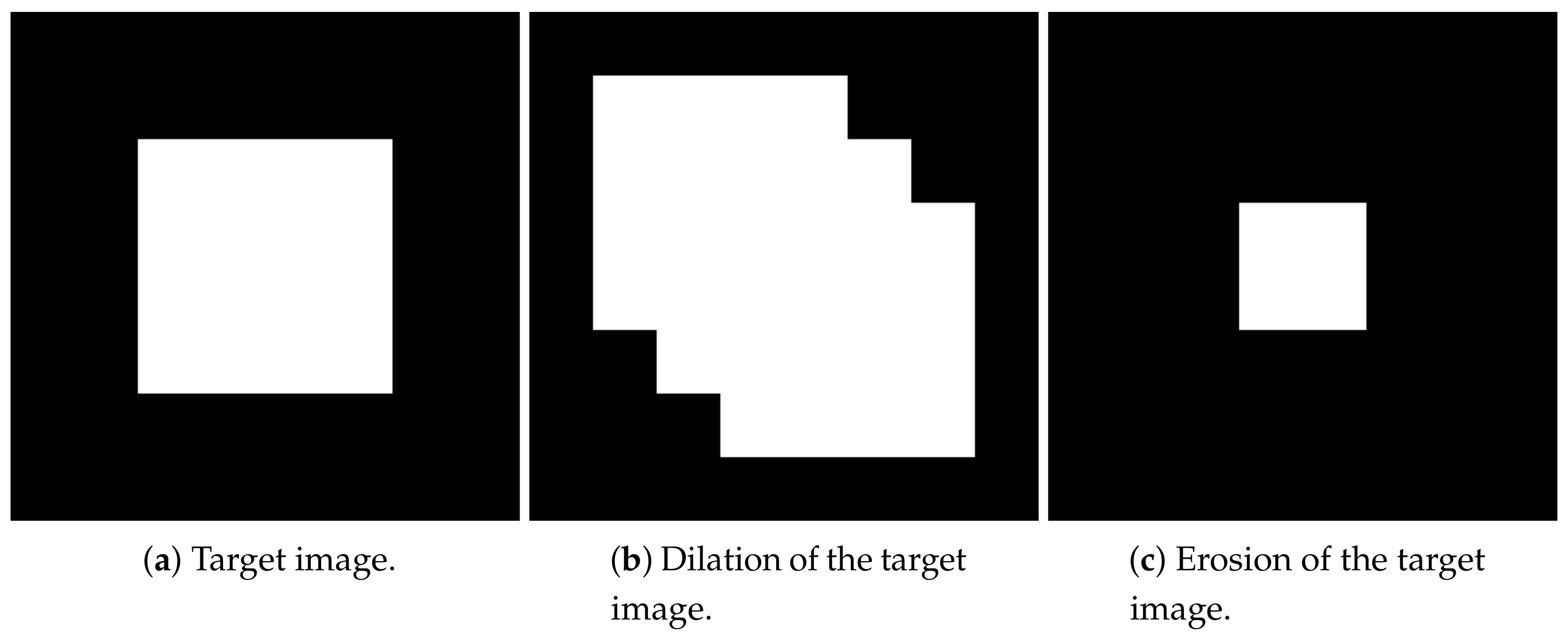
After all of the preparatory work, now we can implement the dilation and erosion operations and obtain the result. Recall that the dilation is in fact the OR operation and the erosion is the AND operation; by applying the quantum OR and AND gates (Figure 3) we can obtain the results of the dilation and erosion, as shown in Figure 10.
In the quantum circuit, we use qubit q [ 1 ] for | G Y , X , q [ 0 ] and q [ 2 ] for | G Y 1 , X 1 and | G Y + 1 , X + 1 , q [ 3 ] q [ 4 ] q [ 5 ] for | Y , q [ 6 ] q [ 7 ] q [ 8 ] for | X and q [ 9 ] for the result | O . To the far left side, the series of Hadamard gates for | Y and | X convert the all | 0 state to | I 0 = 1 2 n Y = 0 2 n 1 | Y X = 0 2 n 1 | X , so as to prepare the initial state of the qubits. At this moment, the position states | Y and | X have not entangled with the color information state | G . The second part of the implementation is the coding subroutine, as discussed in Section 4.2. Through this operation the color information state | G is coded according to the image information. After this step the quantum state of the whole image is obtained.
As we have stated in Section 3.7, we cannot use the same state for different shifting. So, when we use three different states to store the two shifted images, they share the same position qubits. In the third and fourth parts of the circuit the | G Y 1 , X 1 and | G Y + 1 , X + 1 are prepared. After all of the three states are prepared, we apply quantum OR or AND operations to accomplish the dilation and erosion processes, and then measure the results.

5. Results

First, as we prepare and code the color of the pixels into the states, we convert the information of the image to the different quantum states. This procedure is done by the proper coding operation (Figure 6) according to the exact original image. Then, after the dilation and erosion operations, we measure the final states and convert the information back to the pixels in the image. In this way, we obtain the dilated and eroded states via the quantum circuit.
In the previous parts we have already shown how to build the circuits on the IBM QE. Once the circuit is designed, it can be simulated by the simulator or run by the real quantum computers via the IBM cloud. As it is an evolution process of the quantum states, the measurement will destroy the state and makes it collapse to only one possibility. So we need to repeat the process many times to yield final results. By simulating the circuit and analysis the result, we can obtain the dilation and erosion of the target image, as shown in Figure 11.

6. Conclusions

In this work, a quantum algorithm is designed to accomplish the functions of image dilation and erosion. Compared to classical image processing algorithms, the quantum algorithm has several differences. First, rather than encoding the image by bits as in a classical computer, we use entangled qubits to realize this coding process. Second, the operations to the classical bits are straightforward. Because every single classical bit has only two different states. The coefficient of two quantum states can take continuous values rather than only two discrete values. Beside, in a quantum circuit, the qubits are significantly entangled. The change of any qubit will largely influence the states of the other qubits. Both of the features of qubits tremendously contribute to the complexity of quantum algorithms, at the same time, also largely expand the possibilities of the quantum algorithms.
The quantum algorithm in this paper realizes all of the functions of the image dilation and erosion processes via an improved method. It illustrates an efficient way to transplant classical algorithms into the quantum pattern. In this way, we can make full use of the quantum computer and promote understanding of this new field, which holds great potential.

Author Contributions

Conceptualization, H.E., H.H., S.-Y.M. and A.K.; methodology, S.-Y.M., H.E., H.H. and A.K.; software, S.-Y.M.; validation, H.E., H.H. and A.K.; formal analysis, S.-Y.M.; Writing—Original draft preparation, S.-Y.M., A.K., and H.E.; Writing—Review and editing, H.E., H.H. and A.K.; project administration, H.E., H.H. and A.K. All authors have read and agreed to the published version of the manuscript.

Funding

This research received no external funding.

Conflicts of Interest

The authors declare no conflict of interest.

References

  1. Baxes, G.A. Digital Image Processing: Principles and Applications; John Wiley & Sons: New York, NY, USA, 1994. [Google Scholar]
  2. Ngan, K.N.; Meier, T.; Chai, D. Model-Based Coding. In Advanced Video Coding: Principles and Techniques: The Content-based Approach; Elsevier: Burlington, NJ, USA, 1999; Volume 7, pp. 183–249. [Google Scholar]
  3. Li, H.; Chen, X.; Xia, H.; Liang, Y.; Zhou, Z. A Quantum Image Representation Based on Bitplanes. IEEE Access 2018, 6, 62396–62404. [Google Scholar] [CrossRef]
  4. Chen, S.; Zhao, M.; Wu, G.; Yao, C.; Zhang, J. Recent Advances in Morphological Cell Image Analysis. Comput. Math. Methods Med. 2012, 2012, 101536. [Google Scholar] [CrossRef] [PubMed] [Green Version]
  5. Anagnostopoulos, C.; Anagnostopoulos, I.; Loumos, V.; Kayafas, E. A License Plate-Recognition Algorithm for Intelligent Transportation System Applications. IEEE Trans. Intell. Transp. Syst. 2006, 7, 377–392. [Google Scholar] [CrossRef]
  6. Zhao, D.; Daut, D. Morphological hit-or-miss transformation for shape recognition. J. Visual Commun. Image Represent. 1991, 2, 230–243. [Google Scholar] [CrossRef] [Green Version]
  7. Zhou, R.G.; Fan, P.; Tan, C.; Hu, W. Quantum gray-scale image dilation/erosion algorithm based on quantum loading scheme. J. Comput. 2018, 29, 220–227. [Google Scholar]
  8. Yuan, S.; Mao, X.; Li, T.; Xue, Y.; Chen, L.; Xiong, Q. Quantum morphology operations based on quantum representation model. Quantum Inf. Process. 2015, 14, 1625–1645. [Google Scholar] [CrossRef]
  9. Barenco, A.; Bennett, C.; Cleve, R.; DiVincenzo, D.; Margolus, N.; Shor, P.; Sleator, T.; Smolin, J.; Weinfurter, H. Elementary gates for quantum computation. Phys. Rev. A 1995, 52, 3457–3467. [Google Scholar] [CrossRef] [PubMed] [Green Version]
  10. Nielsen, M.; Chuang, I. Quantum Computation And Quantum Information; Cambridge University Press: Cambridge, UK, 2010. [Google Scholar]
  11. Yuan, S.; Mao, X.; Chen, L.; Wang, X. Improved Quantum Dilation and Erosion Operations. Int. J. Quantum Inf. 2016, 14. [Google Scholar] [CrossRef]
  12. Srivastava, M.; Moulick, S.R.; Panigrahi, P.K. Quantum image representation through two-dimensional quantum states and normalized amplitude. arXiv, 2015; arXiv:1305.2251v4. [Google Scholar]
  13. Yao, X.-W.; Wang, H.; Liao, Z.; Chen, M.-C.; Pan, J.; Li, J.; Zhang, K.; Lin, X.; Wang, Z.; Luo, Z.; et al. Quantum Image Processing and Its Application to Edge Detection: Theory and Experiment. Phys. Rev. X 2017, 7. [Google Scholar] [CrossRef]
  14. Yan, F.; Iliyasu, A.; Jiang, Z. Quantum Computation-Based Image Representation, Processing Operations and Their Applications. Entropy 2014, 16, 5290–5338. [Google Scholar] [CrossRef] [Green Version]
  15. Miszczak, J.A. Models of quantum computation and quantum programming languages. Bull. Pol. Acad. Sci.-Tech. Sci. 2011, 59, 305–324. [Google Scholar] [CrossRef] [Green Version]
  16. Dragoman, D.; Dragoman, M. Quantum-Classical Analogies; Springer: Berlin/Heidelberg, Germany, 2004. [Google Scholar]
  17. Yang, Y.; Zhao, Q.; Sun, S. Novel Quantum Gray-Scale Image Matching. Optik 2015, 126, 3340–3343. [Google Scholar] [CrossRef]
Figure 1. NOT gates in binary and quantum circuits. (a) NOT gate in a classical binary circuit, which has input c and output c ¯ (the complement state of c). (b) NOT gate in a quantum circuit (X gate), which has input q and output q ¯ .
Applsci 10 04040 g001
Figure 2. The symbols in quantum circuits and truth tables of the five quantum gates.
Applsci 10 04040 g002
Figure 3. The quantum circuits for AND and OR operations where X and Y represent the position information (See the definition of the symbols in Figure 2).
Applsci 10 04040 g003
Figure 4. Quantum circuit for position shifting transformation. The function of the circuit is to add one to the n-qubit number. (a) The position shifting transformation of x. (b) The position shifting transformation of y.
Applsci 10 04040 g004
Figure 5. Quantum operators in the quantum scores of IBM QE. (a) The CNOT gate. The little dot denotes the control qubit and the larger circle with a “+” denotes the target qubit. (b) The “ccX” subroutine, which is actually the Toffoli gate. Letters in the blue blocks denote the different qubits in the multi-qubit operation, like the a and b are the control qubits and the qubit c is the target qubit.
Applsci 10 04040 g005
Figure 6. The “coding” subroutine. Letters in the blue blocks denote the different qubits in this multi-qubit operation, where a is the qubit for color information, | G ; the position qubits | Y and | X consist of bcd and efg (note that the letters in a specific operation are irrelevant between different operations, they only distinguish different qubits within the operations). The diagram in the middle shows the composition in quantum IBM Q experience, and the counterpart in the quantum circuit notation is shown on the right.
Applsci 10 04040 g006
Figure 7. Structure element.
Applsci 10 04040 g007
Figure 8. The “add 1” subroutine, to add one to a three-bit binary number. The number is denoted by the qubits as ( abc ) b . As explained before (Figure 5b), the “ccX” gate is the Toffoli gate in IBM quantum score with a and c are control qubits while c is the target. The green X gate is the quantum NOT gate, which simply flips the quantum state.
Applsci 10 04040 g008
Figure 9. The “sub 1” subroutine, to subtract one from a three-bit binary number. The number is denoted by the qubits as ( abc ) b . The “”ccX” gate is the Toffoli gate (Figure 5b). Where the qubits denoted by “a” and “b” are control qubits while “c” is the target.
Applsci 10 04040 g009
Figure 10. The circuits for dilation and erosion operation to the image (Equation (13)) by the structure element shown by Figure 7. The qubit q [ 1 ] is for | G Y , X , q [ 0 ] for | G Y 1 , X 1 , q [ 2 ] for | G Y , X , q [ 3 ] q [ 4 ] q [ 5 ] for | Y , q [ 6 ] q [ 7 ] q [ 8 ] for | X and q [ 9 ] for the result | O . To the very left side the Hadamard gates for | Y and | X convert the all | 0 state to | I 0 = 1 2 n Y = 0 2 n 1 | Y X = 0 2 n 1 | X . The “coding” subroutine can code the | G Y , X by the location states while retain the quantum states for position qubits after the operation. The blue blocks with “H” are the Hadamard gates, and the yellow blocks with “id” are identical operations that actually do nothing to the qubits. They are put there only for the symmetry of the circuit considering the possible errors from applying operations.The subroutines “coding”, “add1” and “sub1” are discussed above. (See Figure 6, Figure 8, and Figure 9). The “cccx” subroutine is simply a NOT gate with three control qubits, which is one more than a normal Toffoli gate, where ac are control qubits and d is the target. The pink blocks denote the measurements, where we can see the grey arrows showing that information is passed to classical bits. Then we can get the result | O in q [ 9 ] which is read out in the classical bit 6.
Applsci 10 04040 g010
Figure 11. The target image and its dilation and erosion according to the structure element in Figure 7. (a) A simple example with 8 × 8 = 64 pixels and the central 4 × 4 = 16 pixels being white and the rest black. (b) The dilated image after applying the dilation operator to the original image. It’s actually the union set of the original image and two images after applying position shifting operator at opposite directions. (c) The eroded image after applying the dilation operator to the original image. It’s the intersection of the original image and two position shifted ones.
Applsci 10 04040 g011

