Article

Reliability Analysis of Layered Soil Slopes Considering Different Spatial Autocorrelation Structures

1
Key Laboratory of Metallogenic Prediction of Nonferrous Metals and Geological Environment Monitoring, Ministry of Education, School of Geosciences and Info-Physics, Central South University, 932 South Lushan Road, Changsha 410083, China
2
Hunan Key Laboratory of Nonferrous Resources and Geological Hazards Exploration, 932 South Lushan Road, Changsha 410083, China
*
Author to whom correspondence should be addressed.
Appl. Sci. 2020, 10(11), 4029; https://doi.org/10.3390/app10114029
Submission received: 25 April 2020 / Revised: 6 June 2020 / Accepted: 8 June 2020 / Published: 11 June 2020
(This article belongs to the Section Earth Sciences)

Abstract

:
It is widely recognized that different geological formations often vary differently in space. Therefore, soil properties from different layers should be modeled by different autocorrelation functions (ACFs) to reflect such soil heterogeneity. However, the same ACFs are frequently used for different soil layers in slope reliability analysis for simplicity purpose in the literature. The present work is a study on the effects of ACFs on the reliability analysis of layered soil slopes, where the soil properties of different layers are considered by different ACFs. Five commonly used classical ACFs and the non-classical Whittle–Matérn model were investigated in this study. Cholesky decomposition and Monte Carlo simulation were used to simulate the spatial variability of the soil properties and estimate the probability of failure (Pf) of slopes, respectively. Illustrative examples with various parametric studies show that when the soil properties from different layers are characterized by the same ACFs, the Pf of the studied slopes is comparable with that estimated using different ACFs for different soil layers. This indicates that the type of ACF has only a small impact on the slope reliability assessment. However, the Pf may be underestimated by the single exponential ACF and overestimated by the cosine exponential ACF. The scale of fluctuation of the soil properties influences the slope reliability more than the ACFs. In addition, the smoothness parameter in the non-classical model has a significant influence on the reliability of the slope, where Pf increases with the increase of the smoothness parameter.

1. Introduction

Soil properties are anisotropic and exhibit spatial variability in nature because of the inherent variation in the mineral composition, formation, and alteration of the environment [1,2,3,4,5,6]. Variability is regarded as the observable characterization of heterogeneity, and ignoring it may overestimate the probability of failure ( P f ) of a slope, thus resulting in conservative slope designs [1,2,7]. An autocorrelation structure can be used to characterize the spatial variability [8,9,10,11], where the correlation between two arbitrary points within the soil is described by an autocorrelation function (ACF) [12,13,14,15]. In geotechnical engineering practice, the autocorrelation structure for a soil property is often determined from a large quantity of measurement data by using geostatistics. Site investigation data, however, is generally limited and sparsely measured because of the timeline and project budget. Accurate estimation of the autocorrelation structure is hence difficult to achieve. To this end, theoretical ACFs with assumed values of scale of fluctuation (SOF) are frequently used as the replacements to model the soil spatial variability in geotechnical probabilistic analysis, e.g., slope reliability analysis. Therefore, it is of great significance to investigate the effects of the autocorrelation structure on slope reliability analysis.
Many published studies have highlighted the effects of the theoretical ACF on slope reliability analysis. For example, Li [8] and Liu [16] systematically compared the effects of five commonly used ACFs on the reliability of soil slopes and seepage flow in an embankment, respectively. The same ACFs and SOFs are used for different soil layers in these studies. However, it might be argued that the SOFs for different soil layers can be different, even though the same ACF is adopted. In view of this observation, Liu [17] investigated the effects of SOFs on the reliability analysis of a layered slope, where soil properties were modeled by the same ACF but different SOFs were taken for different soil layers. It was found that when the difference in SOF between different soil layers is large, the slope reliability assessment results might be overestimated or underestimated. However, since different geological formations often vary differently in space, soil properties from different soil layers should be modeled by different ACFs to reflect the soil heterogeneity. As such, the available studies that generally assume the same ACFs for different soil layers in slope reliability analysis tend to be unreasonable. In addition, as stated by Spry [18] and Li and Lumb [19], the variability of soil properties changes with the soil type and location, and no autocorrelation model is univocally preferable over others on the basis of physical motivations. Hence, how to appropriately consider different autocorrelation structures for different soil layers in the reliability analysis of layered soil slopes is still an open question, which poses a challenge to assess the failure risk precisely.
The aim of this paper was to investigate the effects of ACFs on the reliability analysis of layered soil slopes, where soil properties of different soil layers were considered by different ACFs. Five commonly used ACFs and the non-classical Whittle–Matérn model in the literature were investigated. Cholesky decomposition and Monte Carlo simulation were used to simulate the spatial variability of soil properties and estimate the P f of slopes, respectively. A two-layered cohesive slope and a cohesive–frictional slope with a weak seam were studied to elaborate and compare the effects of multiscale soil spatial variability modeled by different ACFs on slope reliability analysis. Moreover, the influence of various SOFs on reliability analysis was also explored.

2. Reliability Analysis of Spatially Varied Soil Slopes

2.1. Autocorrelation Structure of Spatially Varied Soil Properties

The spatial variability of soil properties indicates that soil properties are heterogeneous, with a certain correlation between two points in space. In general, soil properties are far more correlated at adjacent locations than those far away from each other [20]. The SOF is a quantitative statistical index indicating the range within which the soil properties are correlated [21,22,23]. Therefore, a large SOF implies a uniform soil material while a small one implies a heterogeneous material for which the properties change rapidly [24]. It is worthwhile to point out that, as one of the two extremes of the SOF, when the SOF becomes infinitely large, the soil properties at all locations are completely correlated, which can be characterized by a spatial constant. On the contrary, when the SOF is nearly zero or extremely small, the soil properties present little spatial autocorrelation in space. Furthermore, it is noted that SOF is direction dependent and SOFs in different directions are often not consistent. The SOF in the horizontal direction is generally larger than that in the vertical direction because of the depositional and post-depositional processes during the geological formations. Mathematically, the correlation between soil properties at any two points is governed by the ACF, which is the function of the SOF. Both the ACF and SOF are determined from measurement data by using geostatistics with the following steps [20,25,26,27,28]: (1) Evaluate the sample or experimental ACF from data, and (2) fit the sample ACF with the best correlation function. However, owing to the sparse and limited measurement data in geotechnical engineering, it is usually difficult to accurately determine the ACF and SOF from the measurement data [29,30]. Hence, theoretical ACFs are widely used as replacements to describe the spatial variability of soil properties in the literature [16,23,31]. Since reliability analysis is a kind of simulation, it is acceptable to use the theoretical ACFs in slope reliability analysis. However, it is necessary to discuss the effects of different ACFs and SOFs on slope reliability analysis to further understand the potential ranges of the P f of a slope. As reported in the literature [8,12,18], five theoretical ACFs are commonly used for characterizing the spatial variability of soil properties, as listed in Table 1. In the table, ρ denotes the autocorrelation function, and τ x = | x i x j | and τ y = | y i y j | denote the horizontal and vertical lag distances between two points within the soil unit, respectively. δ h and δ v represent the horizontal and vertical SOFs, respectively. Obviously, these functions are different in their expressions, thus resulting in different autocorrelation structures for soil spatial variability. However, physical differences between these functions are not discussed herein as previous studies have investigated this in detail [8,16], and the purpose of this study was not to simply compare the differences between these ACFs. By contrast, the major aim of the current study was to further examine the effects of the combinations of different ACFs for different soil layers on the reliability analysis of layered slopes, which has not been investigated fully before.

2.2. Random Field Simulation of Spatially Varied Soil Properties

The random field theory is often used to simulate the spatial variability of soil properties to consider its effect on slope reliability analysis [22,32]. The steps of discretization of a random field are briefly introduced as follows: (1) Determine the statistical parameters, such as the mean, standard deviation, ACFs, and SOFs; (2) randomly sample a set of independent standard normal random variables; (3) generate the corresponding correlated standard random variables using some random field generation techniques, such as the Cholesky decomposition method [8], Karhunen–Loève expansion method [17,33], and local average subdivision method [34]; and (4) obtain the cross-correlated non-normal random fields through iso-probabilistic transformation. Interested readers can refer to Vanmarcke [32] and Li [8] for details of the generalization of random fields. In this study, the Cholesky decomposition method was adopted as the technique for the realization of random fields because of its simplicity. In addition, extending the Cholesky decomposition method to layered soils problem is straightforward. One only needs to discretize each of the soil layers into different subdomains, with random field simulation for each subdomain following the general procedure described above. Details for simulating non-stationary random fields for layered slopes are given elsewhere [10].

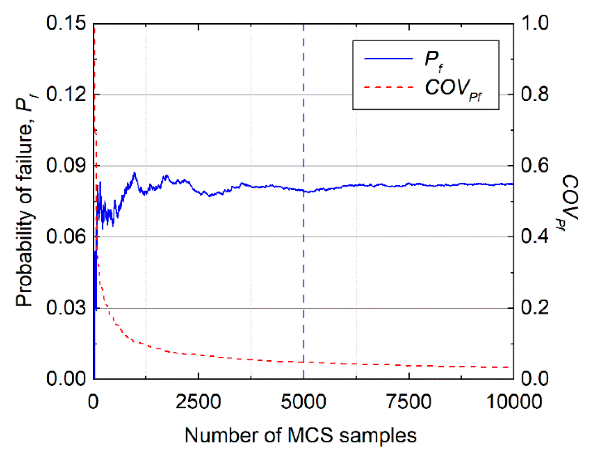
2.3. Monte Carlo Simulation for Slope Reliability Analysis

Regarding the slope reliability analysis considering soil spatial variability, several methods are available in the literature, such as the random limit equilibrium method (RLEM) [35,36], random finite element method (RFEM) [2,37,38], and random smoothed particle hydrodynamics (RSPH) [39]. In this study, the RLEM was adopted because it is conceptually simple and efficient. RLEM generally proceeds with a limit equilibrium method (LEM) within the framework of Monte Carlo simulation (MCS), where LEM is repeatedly performed for vast amounts of random field and/or variable samples to obtain the corresponding slope stability results, for example, the factor of safety (FS) and critical slip surface (CSS). Note that the SLOPE/W [40], which has been verified as an effective and efficient tool for slope stability analysis [8,15,36], was utilized to perform the LEM analysis here. An inhouse MATLAB code, however, was used to simulate random fields and conduct MCS. Each of the samples for a soil property was generated from its probability distribution function (PDF) and correlation structure using the suggested method described in Section 2.2. The variability and non-linearity of soil properties are therefore implicitly considered by the RLEM [3]. With the MCS, the statistics of FS, such as the mean, standard deviation, and distribution of the probability, can be easily obtained. The P f , which is defined as the probability that the FS is less than the unity, is then calculated as:
P f = 1 N m c s i = 1 N m c s I ( F S i < 1 ) ,
where Nmcs is the number of MCS samples; F S i is the FS for the ith MCS sample; and I ( · ) is an indicator function, which is equal to one when the FS is less than the unity and zero otherwise.
To ensure the number of MCS samples is adequate to obtain a relatively precise result, the coefficient of variation of P f , C O V P f , is taken as the indicator to validate the accuracy of the P f , which is expressed as:
C O V P f = 1 P f N m c s P f .
It can be seen from Equation (2) that the accuracy of the P f is inversely proportional to the number of MCS samples N m c s . A small value of C O V P f indicates a good accuracy of the estimated P f , and vice versa. As such, it is often faced with a dilemma of choosing between accuracy and efficiency in practical reliability analysis because N m c s is closely related to the computation efficiency. A reasonable value of the C O V P f is often desired based on the project demand [41]. However, in practice, the balance between calculation accuracy and computation efficiency is warranted, as will be illustrated later.

3. Illustrative Examples

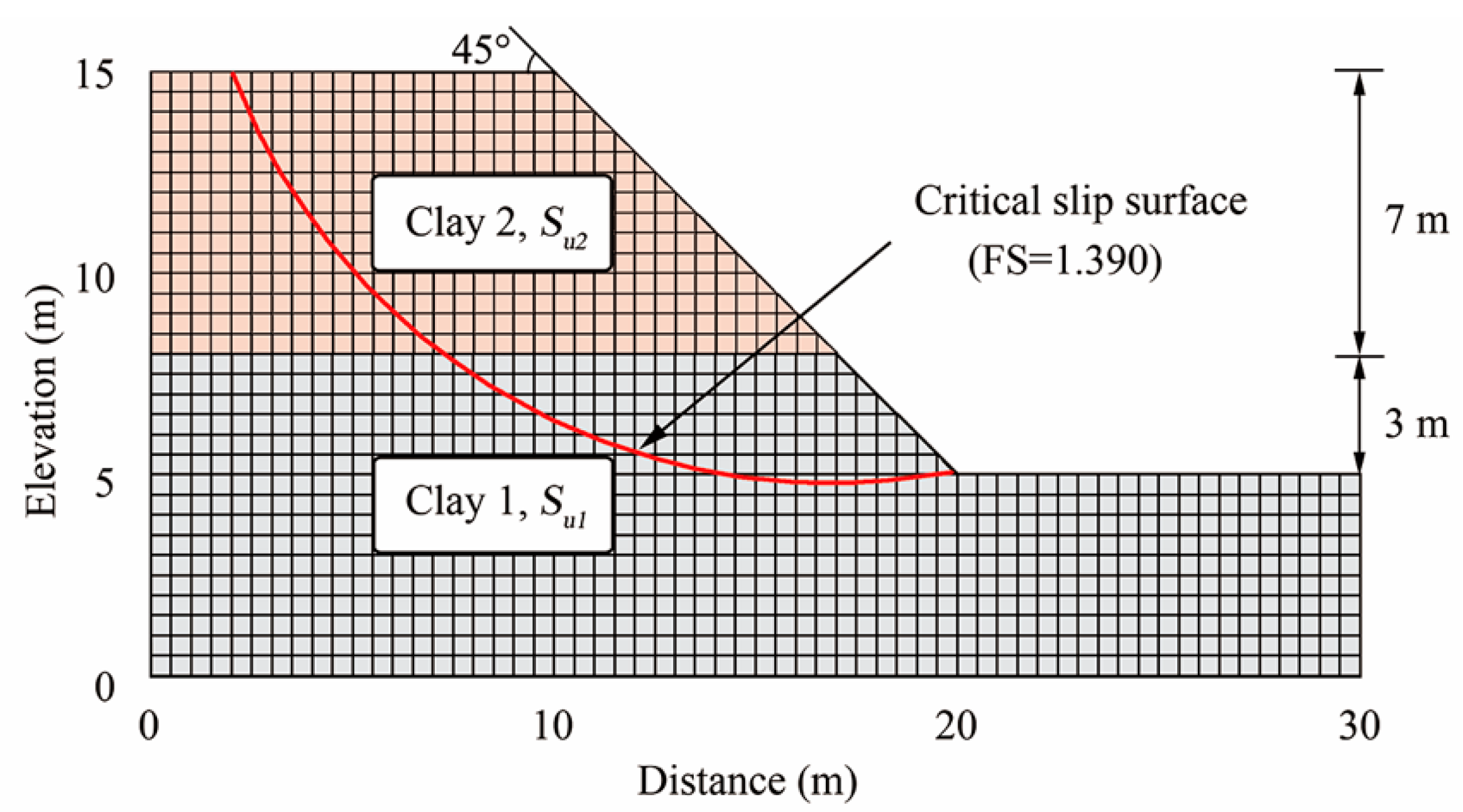
3.1. Example I: A Two-Layered Cohesive Slope

In this section, a two-layered cohesive slope, which has been used to investigate the slope system reliability by Liu [17], is taken as an illustrative example to further examine the effects of autocorrelation structures on the reliability analysis of the slope. It should be noted that the same ACFs were assumed for the two layers. The geometry of the slope and LEM results are schematically plotted in Figure 1. The slope comprises two undrained clay layers, where the substratum is denoted by clay 1 and the upper layer clay 2. The undrained shear strengths of the two clays, which are spatially varied here, are subjected to lognormal distributions. The statistics of the undrained shear strengths are given in Table 2. With the mean values of the soil properties, the FS was calculated as 1.390 using the Bishop’s simplified method and the associated CSS tends to be a toe failure, which is schematically shown in Figure 1. These results are consistent with those reported by Liu [17], showing that the constructed LEM model is accurate enough and can be used with MCS for the subsequent slope reliability analysis. Note that to be consistent with the previous study [17], the unit weight was considered constant.
To further consider the spatial variability of the undrained shear strengths in the established LEM model, the slope domain was then discretized into 1210 random field elements with 1281 nodes, as shown in Figure 1. Based on the midpoints of these elements, the stochastic nature of the undrained shear strengths was simulated by random field theory using the Cholesky decomposition method, as described in Section 2.2. It should be noted that the 1210 elements mean that there are a total of 1210 random variables in each MCS realization. For each of the MCS realizations, the above LEM model was invoked to evaluate the slope stability results. The whole execution of the MCS realizations is termed as the probabilistic slope stability analysis. Since the autocorrelation structure is the key input to the random field simulation, it is, therefore, easy to investigate the effect of the autocorrelation structure on the reliability analysis of the slope with varying ACF types and SOFs by using the probabilistic slope stability analysis. The effects of ACFs and SOFs are studied in the following subsections.

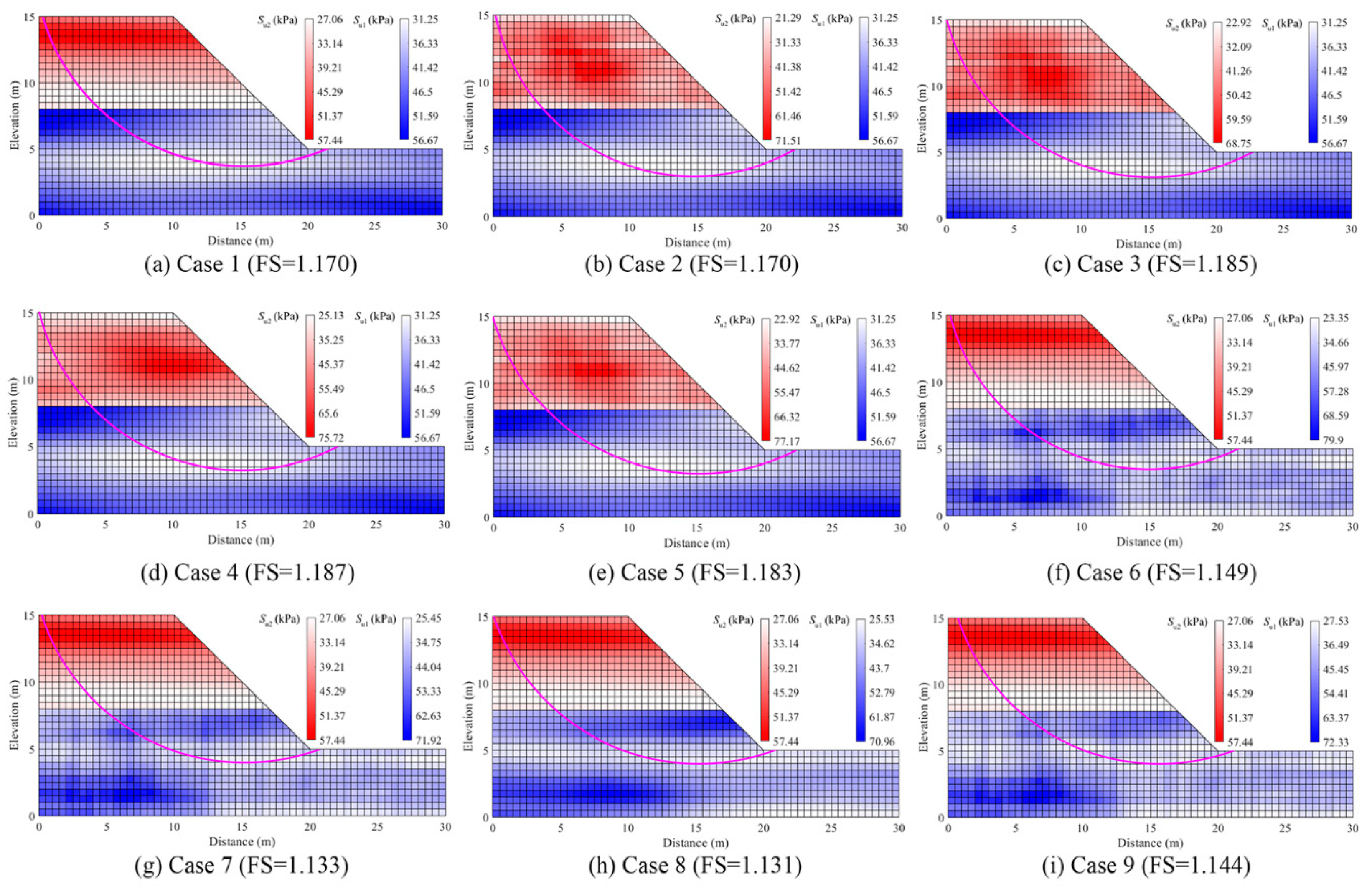
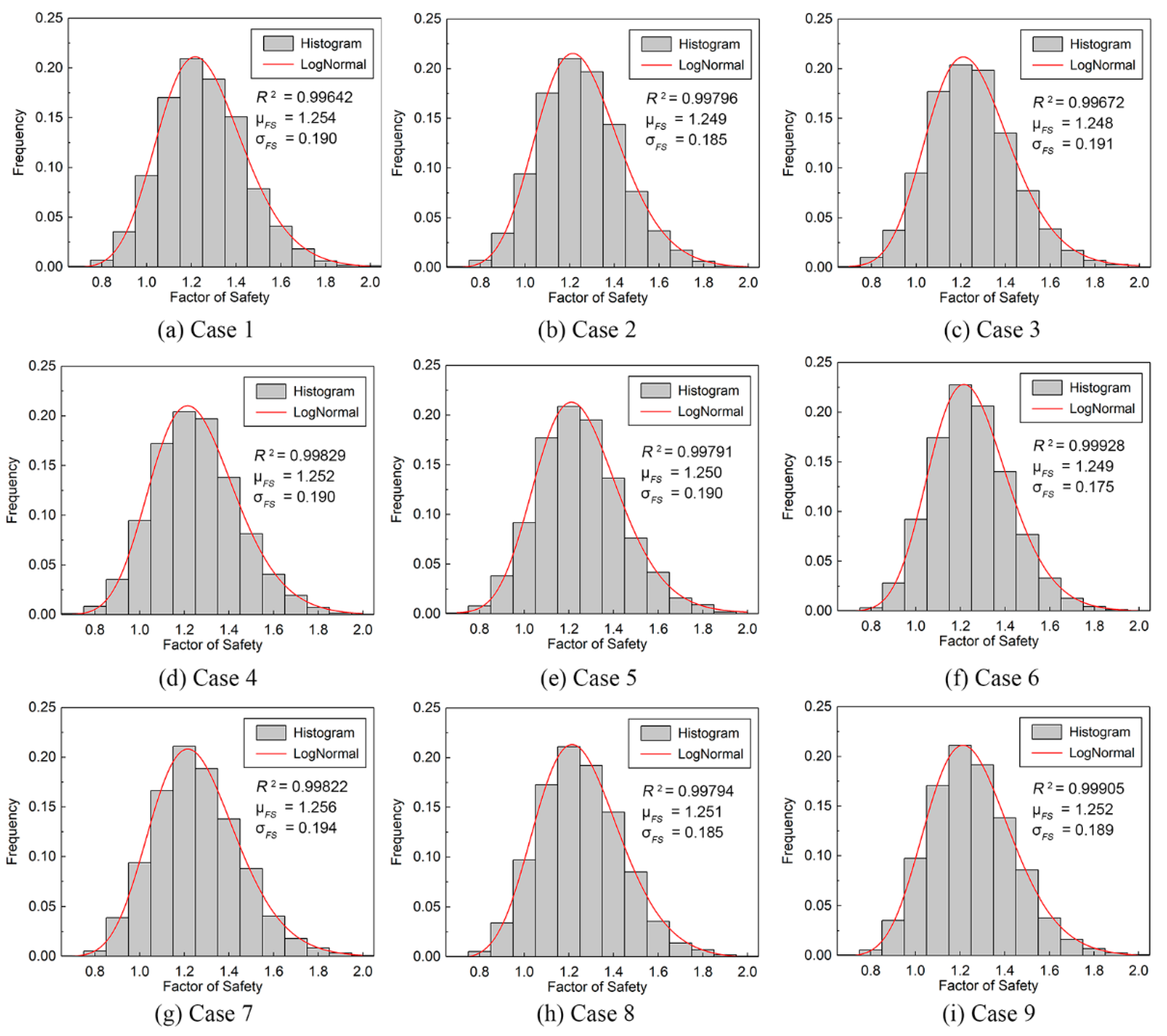
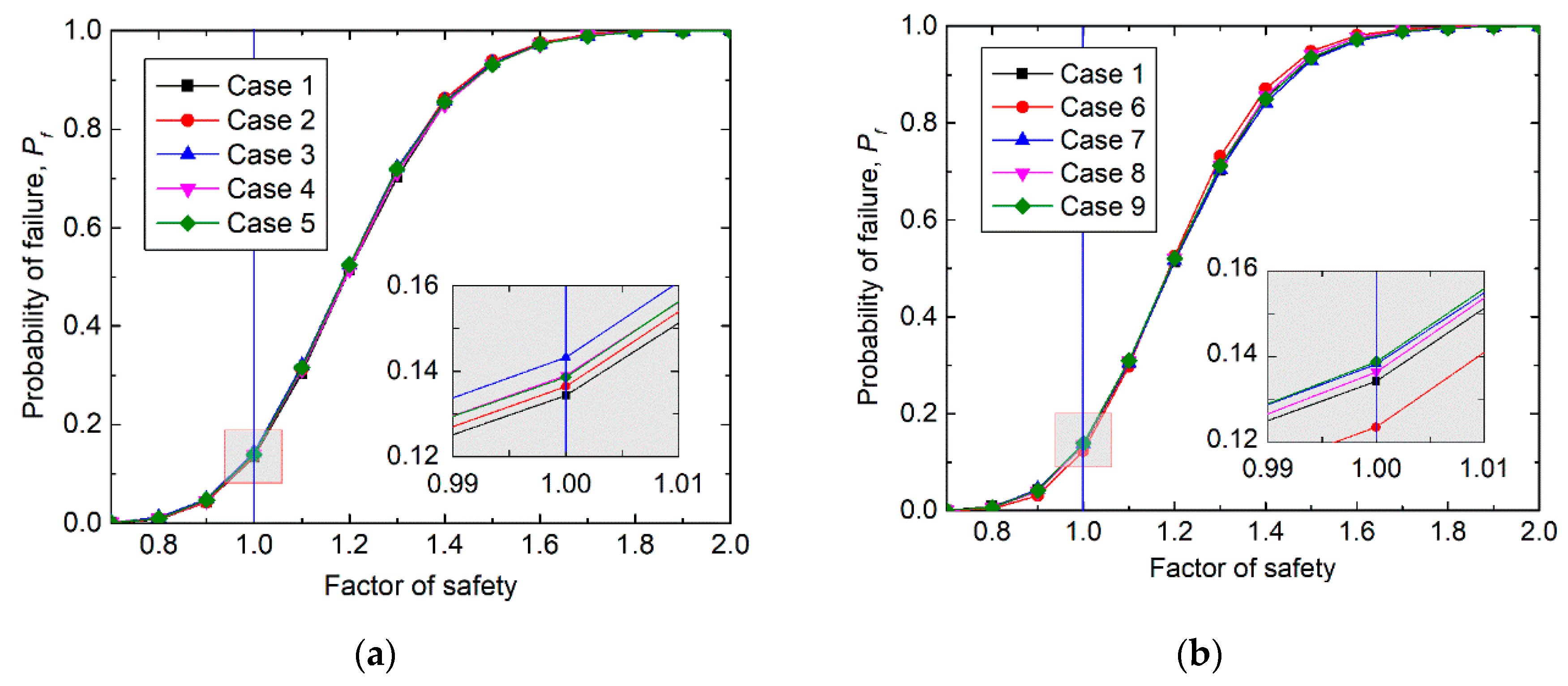
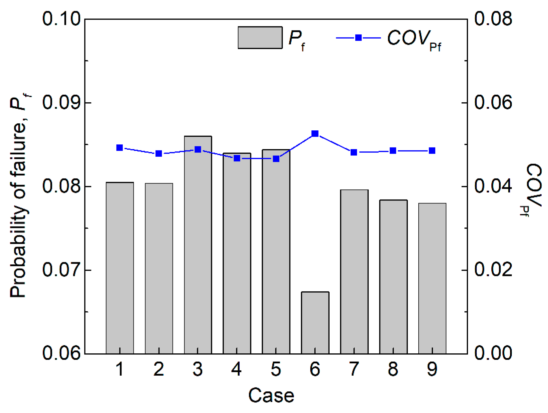
3.1.1. Effects of ACF types on Slope Reliability Analysis

This subsection describes the effects of ACFs on the slope reliability, where the ACF type was taken as the variable in the probabilistic stability analysis. Nine combinations of ACFs for different layers were considered and are listed in Table 3. In each of the nine cases, the ACF was changed among the five types given in Table 1 for clay 1 or clay 2. The cases can be divided into two groups: The change of ACF in the upper stratum (case 1–5) and the lower stratum (case 1 and 6–9). The horizontal SOF, δh, and vertical SOF, δv, were constant here and set as 40 m and 4 m, respectively, which follow a previous study [17] and are from common values of SOF in practice. To simplify the analysis, case 1, where both clay 1 and clay 2 take the SQEF, was considered as the baseline case, as most of the studies available in the literature prefer to use the SQEF to describe the soil spatial variability [4,8,17]. For case 1, the P f was estimated as 8.06 × 10⁻² by the current probabilistic stability model, which is well consistent with that (8.17 × 10⁻²) reported by Liu [17], showing the accuracy of the model. It should be noted that the number of random field realizations plays a crucial role in the accuracy of the result. Here, the MCS size was determined based on a sensitivity study of P f against the number of MCS samples, as shown in Figure 2. It was observed that P f converges to around 8.0 × 10⁻² at the number of around 3000, and remained stable with the increase in the number of the MCS samples. However, a total of 5000 MCS samples were finally used to keep a balance between computation accuracy (e.g., C O V p f < 0.05 ) and efficiency. For other cases, unless otherwise specified, an MCS size of 5000 was also preferably used.
Before directly stepping into the analysis of the effects of ACFs on slope reliability analysis, a visualization comparison of the random fields simulated based on different combinations of ACFs was conducted. Figure 3 plots the typical realizations of random fields for the nine cases, as well as the corresponding slope stability results in terms of CSS and FS. The random fields simulated for different layers are denoted by different colors. For the random field of a specific soil layer, the dark color indicates a large value of the shear strength value and vice versa. It was observed that when ACF is changed, the simulated random fields for the slope is changed accordingly, as well as the corresponding slope stability results. The random fields generated by SQEF and SMF show relatively smoother variation than those obtained from SEF, CEF, and BNF, which shows good consistency with previous studies that assume the same ACF for different soil layers [8]. Compared with the baseline case (case 1), the slope stability results for cases 2–5 where the ACF in the upper layer is respectively taking SEF, CEF, SMF, and BNF remain nearly unchanged whereas the results for cases 6–9 with the ACF in the lower layer respectively taking SEF, CEF, SMF, and BNF have changed to some extent. This shows that the lower layer might dominate the stability of the slope, although the spatial variability for the lower layer is varied. Overall, the assumption of the same ACF for different soil layers might produce conservative (case 1 vs. cases 2–5) or unconservative (case 1 vs. cases 6–9) results.
Statistical analysis of FS was then performed for various cases to further investigate the effects of ACFs on FS and P f based on the MCS results. Figure 4 presents the histograms and PDFs of FS for the nine cases. It can be seen that the FS is well fitted by the lognormal distribution for all cases and there is little difference between the nine cases in terms of the mean, standard deviation, and PDF of FS. However, compared with case 1, the standard deviation for case 2 and 6, where the spatial variability of the two soil layers are described by the SEF and SQEF, is the smallest, showing the large difference between the SEF and SQEF. This finding was also observed by Li [8], _ENREF_36where the same ACF was applied to different soil layers. Besides, Figure 5 compares the cumulative distribution functions (CDFs) of FS for all cases. As can be seen from the figure, the ACF has a minor effect on CDF. To gain more insights into the relative relationships between different ACFs, the locally enlarged images in Figure 5 reveals similar results as Figure 4, where the difference between SEF and SQEF is relatively larger than other combinations of ACFs. The result implies that the P f acquired from the other four ACFs may be overestimated compared with the baseline case, except for case 6.
Figure 6 compares the P f obtained for different cases. As seen from the figure, different combinations of ACFs have different effects on the P f . Generally, the change of ACF in the lower stratum has a greater influence on the P f than that for the upper stratum. Within each group, the results using CEF are relatively larger than those characterized by the other four ACFs. By contrast, the result using SEF is the minimum among the five ACFs. This phenomenon indicates that the P f obtained by the CEF is comparatively more conservative while the SEF may lead to an unconservative estimation. The COV of the P f , C O V P f , shows the opposite trend to the value of P f , which means that smaller P f leads to a greater coefficient of variation with the same MCS size.

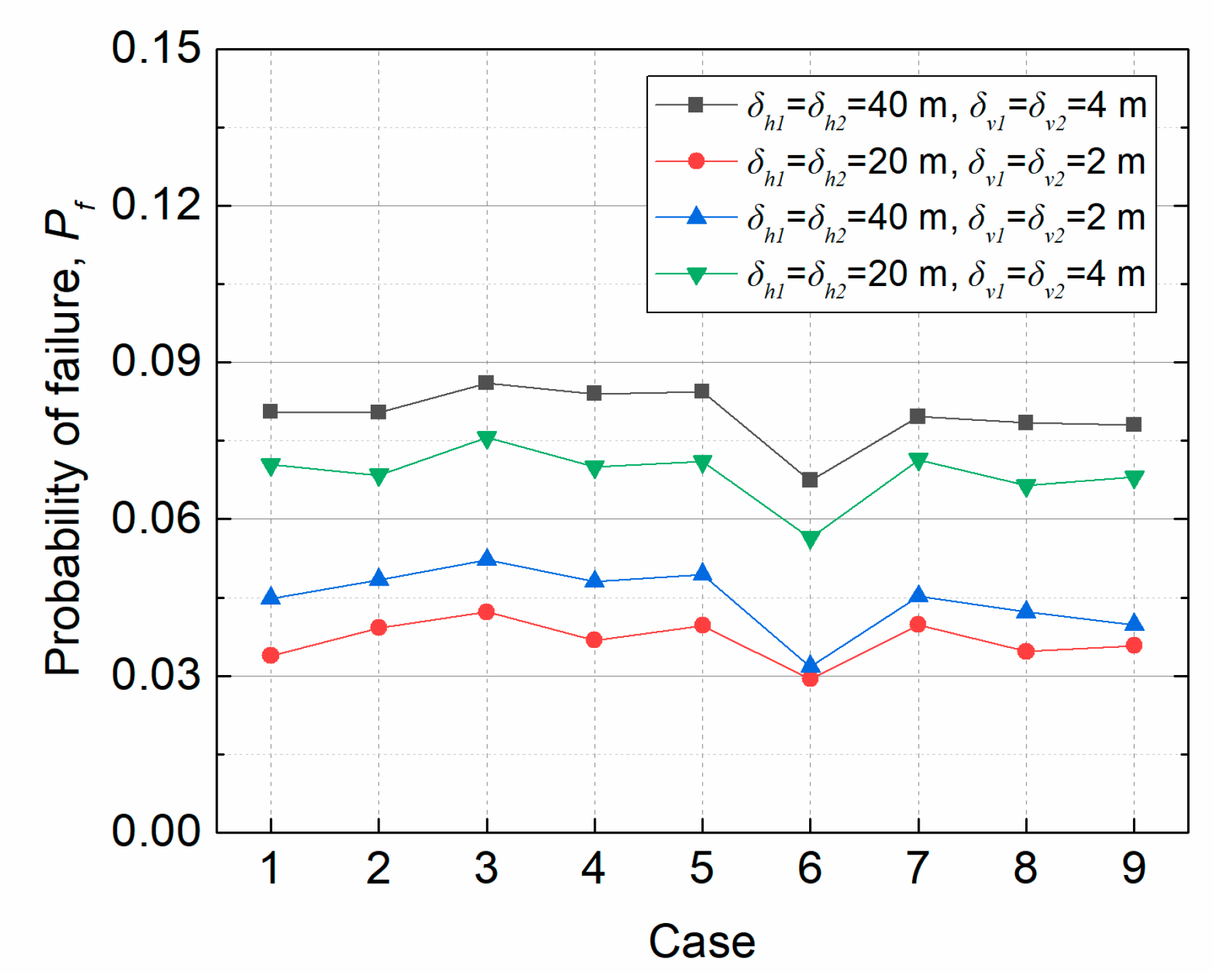
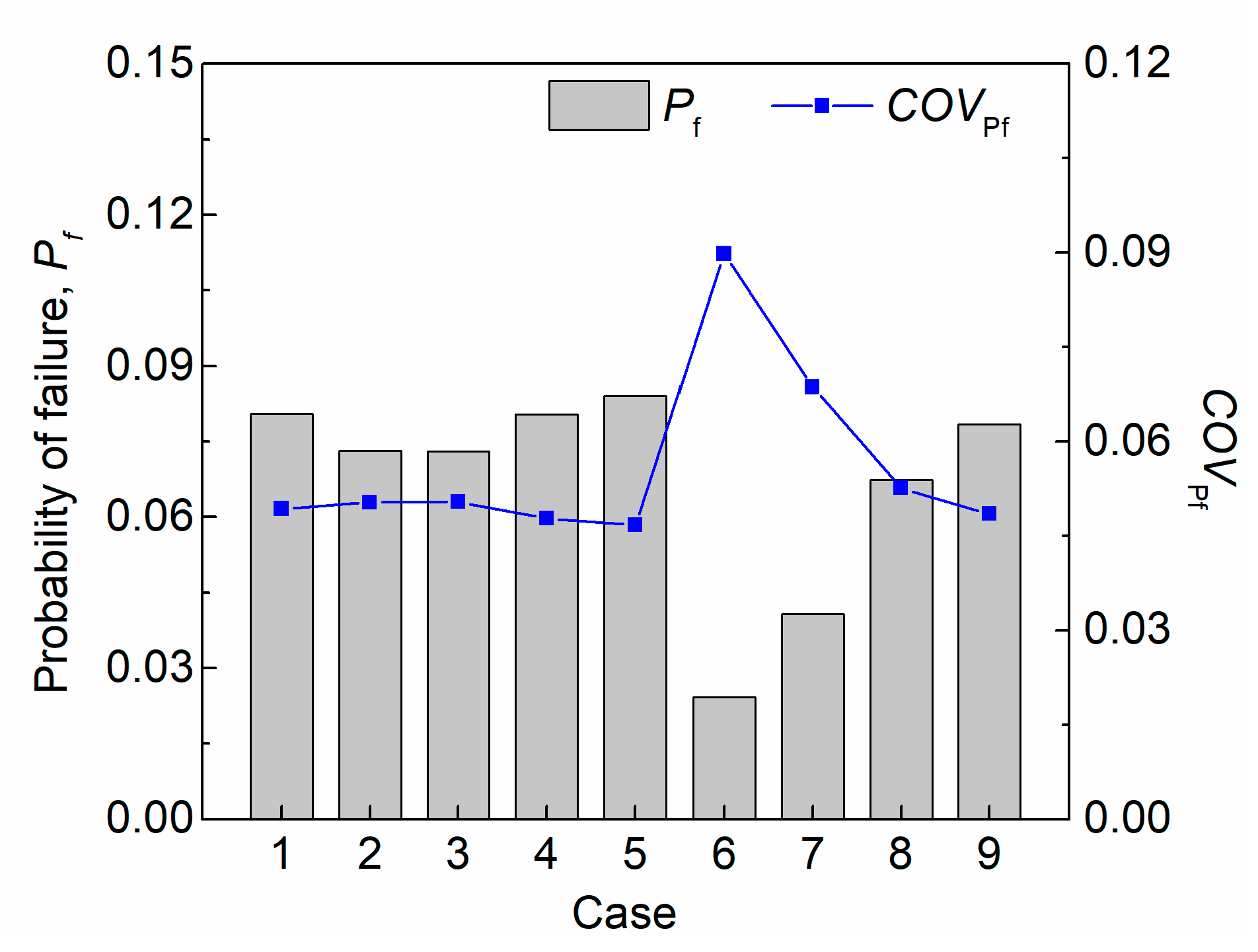
3.1.2. Effect of SOF on Slope Reliability Analysis

This part investigates the effect of SOF on the reliability of the slope. First, the conventional analysis where the same SOFs assumed for different soil layers were investigated, as shown in Figure 7. It is found that the SOF has a significant influence on the failure probability of the slope for different combinations of ACFs. The P f decreases as the vertical scale of fluctuation ( δ v ) or horizontal scale of fluctuation ( δ h ) decreases. In addition, compared with δ h , δ v is more sensitive to the P f . Such observations are expected and consistent with available studies in the literature [8].
Then, the effect of multiple scale SOFs on the reliability of the slope was analyzed, where for different soil layers, the SOFs were different. Various parametric studies on the horizontal and vertical SOFs were investigated, and only one parameter was varied in each study while keeping others as the same as those for the baseline case. For simplicity purposes, only the cases where SEF and CEF were used for describing the soil spatial variability were considered here. Figure 8 shows the influence of the SOFs of clay 1 on the slope reliability evaluation. It shows that P f increases as the horizontal or vertical SOF ( δ h 1 or δ v 1 ) of clay 1 increases for the two cases. Conventional analyses, which assume the same SOFs for different soil layers, can therefore be overestimated or underestimated. When only the SOFs for clay 2 are changed, similar results to those shown in Figure 9 can be observed. However, the P f is not sensitive to the variation of the horizontal SOF δ h 2 , indicating that the SOF in clay 1 has a more significant effect on the P f than the SOF in clay 2 does.

3.2. Example II: A Cohesive–Frictional Slope with a Weak Seam

For further illustration, the study was applied to a cohesive–frictional slope example with a weak seam, which was previously studied by Cheng [42] and Liu [43]. As shown in Figure 10, the slope height is 12.25 m and the slope length is 24.5 m. A 0.5 m weak seam lies below the slope. The shear strengths of the clay and weak seam were subjected to lognormal distributions. Table 4 summarizes the statistics of the parameters of the clay and weak seam. The shear strengths of the two soils were considered spatially variable while the unit weights for the two soils were the same and constant. Based on the mean values of the soil properties, the FS was calculated as 1.528, which was compared with the value of 1.51 reported by Liu [43], and this has validated the accuracy of the deterministic model. In addition, the reliability analysis result based on the SEF ACF is also consistent with that reported by Liu [43], as given in case 1 in Figure 11. Note that the correlation between c and φ is widely acknowledged and is often in a negative value. To ensure the validity of the slope model and to compare it with the previous results, this correlation was not considered here.

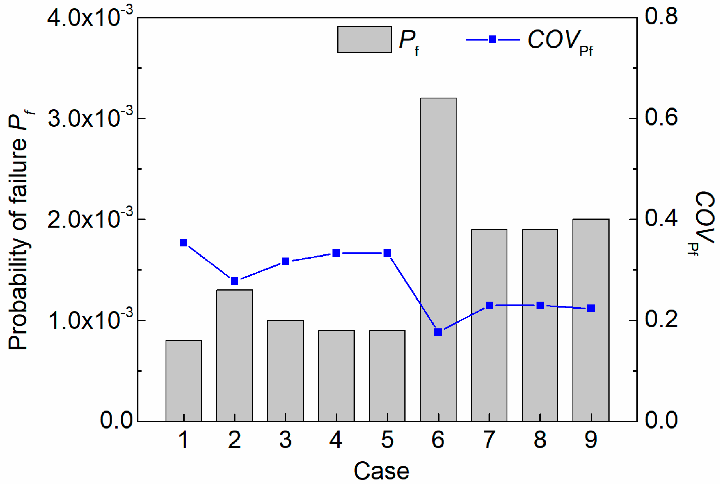
3.2.1. Effect of ACF on Slope Reliability Analysis

This part examines the effect of the ACFs on the reliability of the slope. Similar to example I, nine cases with different ACFs used for different soils were designed. Case 1, where both the clay and the weak seam use the same ACF of SEF, was considered as the baseline case here. Again, for simplicity, the nine cases were classified into two groups: Case 1–5 belong to the first group where SEF is used for the clay and the weak seam uses the other four ACFs. Case 1, 6–9 belong to another group, where SEF is used for the weak seam and the clay uses the other four ACFs. For all cases, the same SOFs are used for different soil layers, with δ h = 20   m and δ v = 4   m . The effect of ACFs on the slope reliability can therefore be easily investigated by changing the ACFs for different soil layers according to the cases in Table 5. Note that the Latin hypercube sampling (LHS) was used here as the level of failure probability is relatively low. The slope reliability results are schematically shown in Figure 11, where the P f values for different cases are signified by the histograms, and the COVs of the P f are plotted by a curved line. In general, different ACFs show different influences on the slope reliability. For the first investigating group (i.e., case 1–5), the difference between the five cases is not significant, showing that the ACF of the weak seam has little influence on the slope reliability analysis. By contrast, the difference between the five cases in the other investigating group (i.e., case 1, 6–9) is comparably significant. Overall, the change of the ACF in the clay has little influence on the slope reliability results, but the reliability results can be significantly different when opposite ACFs are used (e.g., case 2 vs. 6). In addition, the difference of the results obtained using SEF and CEF (i.e., case 2 vs. 6) is the largest among all cases, which shows good consistency with example I.

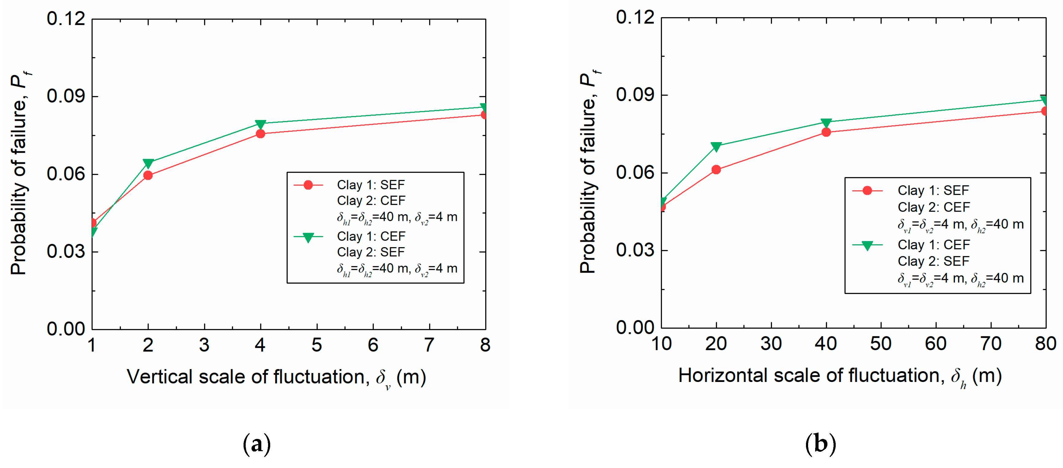
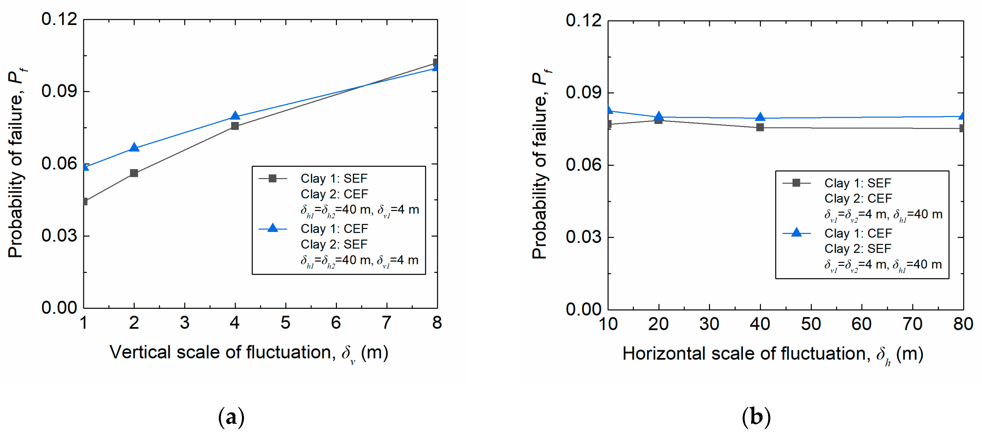
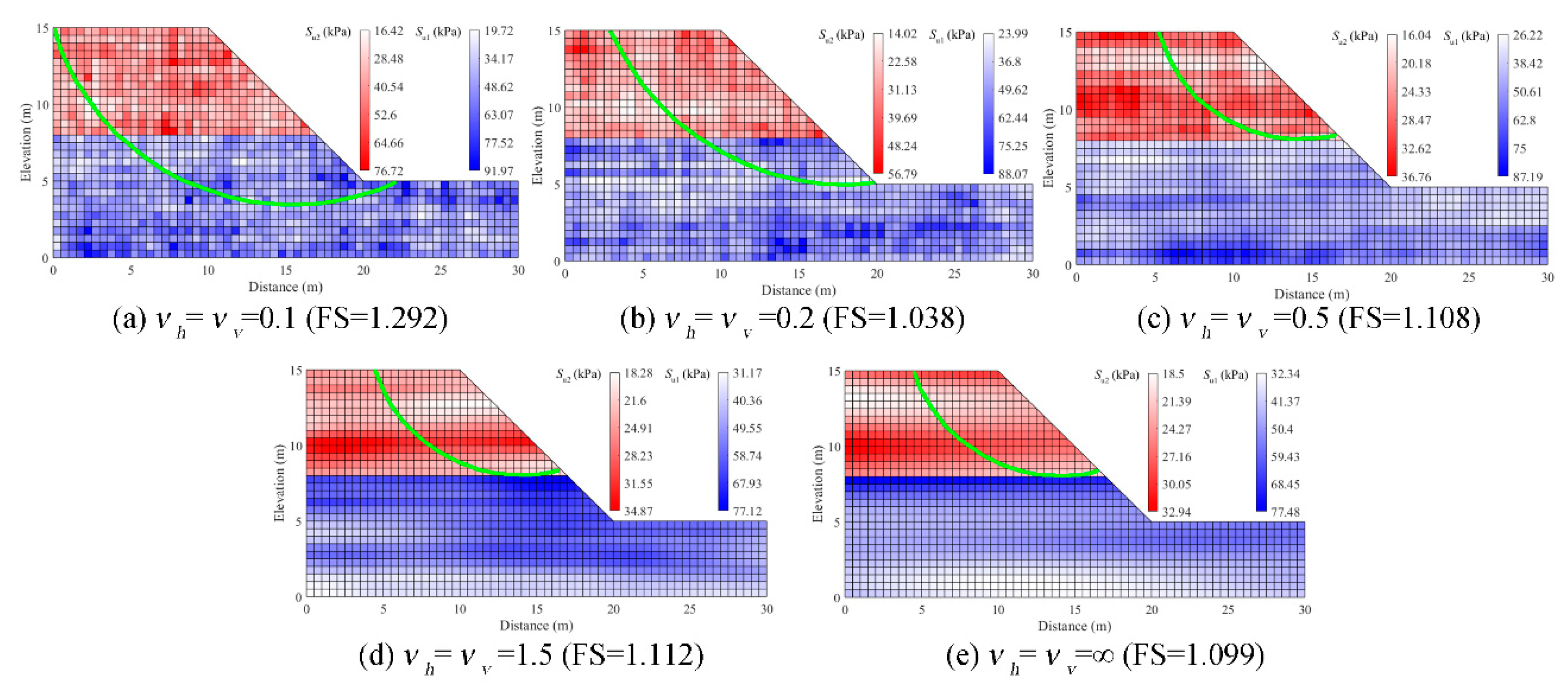
3.2.2. Effect of SOF on Slope Reliability Analysis

This part compares the effect of the vertical SOF ( δ v ) on the reliability of the slope considering that δ v is more sensitive than the horizontal SOF ( δ h ). Similar to example 1, the SEF and CEF are considered here, with each study varying one parameter while keeping the others the same as those for the baseline case. The results are given in Table 6. It shows that P f increases as the vertical SOF of clay increases for the two situations (case 1 vs. 2 and case 3 vs. 4), but the P f remains the same as the vertical SOF of the weak seam increases (case 5 vs. 6 and case 7 vs. 8). The reason may be that the thickness (0.5 m) of the weak seam is far less than the vertical SOF, which leads to the variation of the vertical SOF exerting little influence on the P f .

4. Discussion

Besides five commonly used classical ACF models, the non-classical ACF model, which contains two or more parameters, is usually used to fit two sample path features, such as the SOF and smoothness [13,44]. Ching [44] adopted the Whittle–Matérn (W–M) and powered exponential (PE) models to represent the real soil data and verified that the smoothness parameter has an effect on P f for some geotechnical problems. To reveal whether the non-classical ACF model would affect the reliability of the layered slope, the W–M model, which has been advocated as a general model for soil variogram [45], was used during the realizations of random fields. The Whittle–Matérn model can be expressed as follows [44,46,47]:
ρ ( τ ) = 2 Γ ( υ ) · ( π · Γ ( υ + 0.5 ) · τ Γ ( υ ) · δ ) υ K υ ( 2 π · Γ ( υ + 0.5 ) · τ Γ ( υ ) · δ ) ,
where υ is the smoothness parameter; Γ ( · ) denotes the Gamma function; K υ denotes the modified Bessel function of the second kind with order υ ; and τ is the lag distances between two points. Details for constructing a two-dimension random field can be found in Ching and Phoon [13]. The SEF, SMF, and SQEF are the special case of the W–M model with υ = 0.5, 1.5 and ∞, respectively [13,44]. For illustration, the slope in example I was utilized to investigate the effect of υ on the reliability analysis of the layered slopes. It is noted that the anisotropy of the smoothness was not considered here, which indicates that the smoothness parameters in the horizontal and vertical directions are the same within the realization of the model. Figure 12 plots the typical realization of the random fields with different υ . It can be observed that the random fields with a low υ value (Figure 12a,b) show a relatively rough distribution of the undrained shear strength. With the increase of υ , the random fields become smoother (Figure 12c–e), which may be more suitable to represent the natural property of soils.
Nine cases of combinations of different υ for different layers are listed in Table 7. These cases can be divided into two groups, the change of υ in the upper stratum (Case 1–5) and lower stratum (Case 1 and 6–9). Case 1 is considered as the baseline case. The rest of the parameters of the model are consistent with example I. Figure 13 shows that the slope reliability results for case 1–5 remain nearly unchanged with the increase of the υ . In the lower layer (Case 1, 6–9), P f increases with the increase of υ , showing a significant influence on the slope reliability. This result also further validates that the lower layer might dominate the stability of the slope.

5. Summary and Conclusions

The purpose of this paper was to investigate the effects of ACFs on the reliability analysis of layered soil slopes, where soil properties of different soil layers are considered by different ACFs. Five commonly used classical ACFs and a non-classical model (W–M model) in the literature constituting different cases were investigated. A two-layered cohesive slope and a cohesive–frictional slope with a weak seam were studied to illustrate the influence of ACFs and SOFs on the reliability analysis. The results showed that the autocorrelation structures generally have an influence on the reliability analysis of layered slopes. The ACF types have little influence on the slope reliability, whereas the SOFs can significantly affect the reliability assessment. When different ACFs are used for different soil layers, the reliability results are not sensitive to the change of ACFs either in the lower or upper soil stratum. However, it was found that when the SEF and CEF are used, the reliability results can be quite different from those estimated from other ACFs or from the conventional analysis. The reliability results from SEF tend to be underestimated, whereas those from the CEF can be overestimated. Furthermore, for layered slopes, there might be different SOFs for different soil layers, suggesting that the conventional reliability analysis with the same SOFs for different soil layers could be biased. It is also noted from the two examples that when two ACFs used for two soil layers are exchanged, the reliability results can be significantly varied. In the W–M model, the reliability of the slope would be affected by the smoothness parameter, where the probability of failure increases with the increase of the smoothness parameter to some extent.
To conclude, owing to the nature of soil spatial variability, the autocorrelation structure plays an important role in slope reliability analysis and should be carefully considered in practical reliability analysis. To accurately assess the reliability of slopes, geodata from the field and/or laboratory tests should preferably be used to estimate the autocorrelation structure. For practical situations where geotechnical data is limited, sensitivity studies are necessary in order to obtain a desirable safety assessment. The current study, therefore, can serve as a useful reference for such situations. It is also worthwhile to point out that only lognormal distributions were considered for describing the stochastic nature of soil properties in the current study. This can be a potential limit of this study because lognormal is always skewed to the right and the degree of skewness increases as the standard deviation increases for a fixed mean value. Furthermore, it is also worthwhile to study the effect of slope geometry uncertainty in the future study.

Author Contributions

Conceptualization, L.L.; Data curation, Y.L. and J.L.; Investigation, Y.L. and J.L.; Project administration, S.Z. and L.L.; Software, J.L.; Supervision, S.Z.; Writing—original draft, J.L. and Y.L.; Writing—review & editing, S.Z. and L.L. All authors have read and agreed to the published version of the manuscript.

Funding

This research was funded by grants from the Natural Science Foundation of China (Project Nos. 41902291 and 41872186).

Conflicts of Interest

The authors declare no conflict of interest.

References

  1. Uzielli, M.; Lacasse, S.; Nadim, F.; Phoon, K.K. Soil variability analysis for geotechnical practice. In Characterization & Engineering Properties of Natural Soils; CRC Press: Boca Raton, FL, USA, 2006. [Google Scholar]
  2. Griffiths, D.V.; Huang, J.; Fenton, G.A. Influence of spatial variability on slope reliability using 2-D random fields. J. Geotech. Geoenviron. 2009, 10, 1367–1378. [Google Scholar] [CrossRef] [Green Version]
  3. Cho, S.E. Probabilistic analysis of seepage that considers the spatial variability of permeability for an embankment on soil foundation. Eng. Geol. 2012, 133, 30–39. [Google Scholar] [CrossRef]
  4. Wang, B.; Liu, L.; Li, Y.; Jiang, Q. Reliability analysis of slopes considering spatial variability of soil properties based on efficiently identified representative slip surfaces. Int. J. Rock Mech. Rock Eng. 2020. [Google Scholar] [CrossRef]
  5. Liu, L.L.; Cheng, Y.M.; Pan, Q.J.; Dias, D. Incorporating stratigraphic boundary uncertainty into reliability analysis of slopes in spatially variable soils using one-dimensional conditional Markov chain model. Comput. Geotech. 2020, 118, 103321. [Google Scholar] [CrossRef]
  6. Pan, Q.J.; Qu, X.R.; Liu, L.L.; Dias, D. A sequential sparse polynomial chaos expansion using Bayesian regression for geotechnical reliability estimations. Int. J. Numer. Anal. Methods Geomech. 2020, 44, 874–889. [Google Scholar] [CrossRef]
  7. Santoso, A.M.; Phoon, K.K.; Quek, S.T. Effects of soil spatial variability on rainfall-induced landslides. Comput. Struct. 2011, 89, 893–900. [Google Scholar] [CrossRef]
  8. Li, D.Q.; Jiang, S.H.; Cao, Z.J.; Wei, Z.; Zhou, C.B.; Zhang, L.M. A multiple response-surface method for slope reliability analysis considering spatial variability of soil properties. Eng. Geol. 2015, 187, 60–72. [Google Scholar] [CrossRef]
  9. Qi, X.H.; Li, D.Q. Effect of spatial variability of shear strength parameters on critical slip surfaces of slopes. Eng. Geol. 2018, 239, 41–49. [Google Scholar] [CrossRef]
  10. Jiang, S.H.; Huang, J.S. Efficient slope reliability analysis at low-probability levels in spatially variable soils. Comput. Geotech. 2016, 75, 18–27. [Google Scholar] [CrossRef]
  11. Hicks, M.; Li, Y. Influence of length effect on embankment slope reliability in 3D. Int. J. Numer. Anal. Methods Geomech. 2018, 42, 891–915. [Google Scholar]
  12. Phoon, K.K.; Quek, S.T.; An, P. Identification of Statistically Homogeneous Soil Layers Using Modified Bartlett Statistics. J. Geotech. Geoenviron. 2003, 129, 649–659. [Google Scholar] [CrossRef]
  13. Ching, J.; Phoon, K.-K. Impact of Autocorrelation Function Model on the Probability of Failure. J. Eng. Mech. 2019, 145, 4018123. [Google Scholar] [CrossRef]
  14. Luo, N.; Bathurst, R.J. Probabilistic analysis of reinforced slopes using RFEM and considering spatial variability of frictional soil properties due to compaction. Georisk Assess. Manag. Risk Eng. Syst. Geohazards 2018, 12, 87–108. [Google Scholar] [CrossRef]
  15. Low, B.K.; Lacasse, S.; Nadim, F. Slope reliability analysis accounting for spatial variation. Georisk Assess. Manag. Risk Eng. Syst. Geohazards 2007, 1, 177–189. [Google Scholar] [CrossRef]
  16. Liu, L.L.; Cheng, Y.M.; Jiang, S.H.; Zhang, S.H.; Wang, X.M.; Wu, Z.H. Effects of spatial autocorrelation structure of permeability on seepage through an embankment on a soil foundation. Comput. Geotech. 2017, 87, 62–75. [Google Scholar] [CrossRef]
  17. Liu, L.L.; Zhang, S.H.; Cheng, Y.M. Advanced reliability analysis of slopes in spatially variable soils using multivariate adaptive regression splines. Geosci. Front. 2019, 10, 671–682. [Google Scholar] [CrossRef]
  18. Spry, M.J.; Kulhawy, F.H.; Grigoriu, M.D. Reliability-Based Foundation Design for Transmission Line Structures: Volume 1, Geotechnical Site Characterization Strategy: Final Report; Electric Power Research Institute: Palo Alto, CA, USA, 1988. [Google Scholar]
  19. Li, K.S.; Lumb, P. Probabilistic design of slopes. Can. Geotech. J. 1987, 24, 520–535. [Google Scholar] [CrossRef]
  20. Guo, X.; Dias, D.; Pan, Q. Probabilistic stability analysis of an embankment dam considering soil spatial variability. Comput. Geotech. 2019, 113, 103093. [Google Scholar] [CrossRef]
  21. Deutsch, C. Geostatistical Reservoir Modeling; Oxford University Press: Oxford, UK, 2002. [Google Scholar]
  22. Uzielli, M.; Vannucchi, G.; Phoon, K.K. Random field characterisation of stress-nomalised cone penetration testing parameters. Géotechnique 2005, 55, 3–20. [Google Scholar] [CrossRef]
  23. Fenton, G.A.; Griffiths, D.V. Risk Assessment in Geotechnical Engineering; John Wiley & Sons, Inc.: Hoboken, NJ, USA, 2008. [Google Scholar]
  24. Christian John, T.; Ladd Charles, C.; Baecher Gregory, B. Reliability Applied to Slope Stability Analysis. J. Geotech. Eng. 1994, 120, 2180–2207. [Google Scholar] [CrossRef]
  25. Guo, X.; Dias, D.; Carvajal, C.; Peyras, L.; Breul, P. Reliability analysis of embankment dam sliding stability using the sparse polynomial chaos expansion. Eng. Struct. 2018, 174, 295–307. [Google Scholar] [CrossRef]
  26. Guo, X.; Dias, D.; Carvajal, C.; Peyras, L.; Breul, P. A comparative study of different reliability methods for high dimensional stochastic problems related to earth dam stability analyses. Eng. Struct. 2019, 188, 591–602. [Google Scholar] [CrossRef]
  27. Guo, X.; Du, D.; Dias, D. Reliability analysis of tunnel lining considering soil spatial variability. Eng. Struct. 2019, 196, 109332. [Google Scholar] [CrossRef]
  28. Oliver, M.A.; Webster, R. Basic Steps in Geostatistics: The Variogram and Kriging; Springer International Publishing: Cham, Switzerland, 2015. [Google Scholar]
  29. Wang, Y.; Zhao, T.; Phoon, K.K. Statistical inference of random field auto-correlation structure from multiple sets of incomplete and sparse measurements using Bayesian compressive sampling-based bootstrapping. Mech. Syst. Signal Process. 2019, 124, 217–236. [Google Scholar] [CrossRef]
  30. Wang, Y.; Zhao, T.; Phoon, K.K. Direct simulation of random field samples from sparsely measured geotechnical data with consideration of uncertainty in interpretation. Can. Geotech. J. 2018, 55, 862–880. [Google Scholar] [CrossRef]
  31. Wang, Y.; Akeju, O.V.; Zhao, T. Interpolation of spatially varying but sparsely measured geo-data: A comparative study. Eng. Geol. 2017, 231, 200–217. [Google Scholar] [CrossRef]
  32. Vanmarcke, E.H. Random Fields Analysis and Synthesis; MIT Press: Cambridge, MA, USA, 1983. [Google Scholar]
  33. Phoon, K.K.; Huang, H.W.; Quek, S.T. Comparison between Karhunen-Loeve and wavelet expansions for simulation of Gaussian processes. Comput. Struct. 2004, 82, 985–991. [Google Scholar] [CrossRef]
  34. Fenton, G.A.; Vanmarcke, E.H. Simulation of random fields via local average subdivision. J. Eng. Mech. 1990, 116, 1733–1749. [Google Scholar] [CrossRef] [Green Version]
  35. Jiang, S.H.; Huang, J.; Yao, C.; Yang, J. Quantitative risk assessment of slope failure in 2-D spatially variable soils by limit equilibrium method. Appl. Math. Model. 2017, 47, 710–725. [Google Scholar] [CrossRef]
  36. Cho, S.E. Probabilistic Assessment of slope stability that considers the spatial variability of soil properties. J. Geotech. Geoenviron. 2010, 136, 975–984. [Google Scholar] [CrossRef]
  37. Griffiths, D.V.; Fenton, G.A. Probabilistic slope stability analysis by finite elements. J. Geotech. Geoenviron. 2004, 130, 507–518. [Google Scholar] [CrossRef] [Green Version]
  38. Huang, J.; Griffiths, D.V.; Fenton, G.A. System reliability of slopes by RFEM. Soils Found. 2010, 50, 343–353. [Google Scholar] [CrossRef] [Green Version]
  39. Wang, Y.; Qin, Z.; Liu, X.; Li, L. Probabilistic analysis of post-failure behavior of soil slopes using random smoothed particle hydrodynamics. Eng. Geol. 2019, 261, 105266. [Google Scholar] [CrossRef]
  40. GEO-SLOPE International Ltd. Stability Modeling With SLOPE/W: An Engineering Methodology [Computer Program]; GEO-SLOPE International Ltd.: Calgary, AB, Canada, 2012. [Google Scholar]
  41. Shooman, M. Probabilistic Reliability—An Engineering Approach; McGraw-Hill: New York, NY, USA, 1968. [Google Scholar]
  42. Cheng, Y.M.; Li, L.; Chi, S.C. Performance studies on six heuristic global optimization methods in the location of critical slip surface. Comput. Geotech. 2007, 34, 462–484. [Google Scholar] [CrossRef]
  43. Liu, X.; Li, D.Q.; Cao, Z.J.; Wang, Y. Adaptive Monte Carlo simulation method for system reliability analysis of slope stability based on limit equilibrium methods. Eng. Geol. 2020, 264, 105384. [Google Scholar] [CrossRef]
  44. Ching, J.; Phoon, K.-K.; Stuedlein, A.W.; Jaksa, M. Identification of sample path smoothness in soil spatial variability. Struct. Saf. 2019, 81, 101870. [Google Scholar] [CrossRef]
  45. Marchant, B.P.; Lark, R.M. The Matérn variogram model: Implications for uncertainty propagation and sampling in geostatistical surveys. Geoderma 2007, 140, 337–345. [Google Scholar] [CrossRef]
  46. Pardo-Iguzquiza, E.; Chica-Olmo, M. Geostatistics with the Matern semivariogram model: A library of computer programs for inference, kriging and simulation. Comput. Geosci. 2008, 34, 1073–1079. [Google Scholar] [CrossRef]
  47. Liu, W.F.; Leung, Y.F.; Lo, M.K. Integrated framework for characterization of spatial variability of geological profiles. Can. Geotech. J. 2016, 54, 47–58. [Google Scholar] [CrossRef]
Figure 1. Slope geometry and deterministic slope stability analysis results for example I.
Applsci 10 04029 g001
Figure 2. Number of Monte Carlo simulation (MCS) samples versus P f and C O V P f .
Applsci 10 04029 g002
Figure 3. Typical realizations of random fields underlying S u 1 and S u 2 associated slope stability results (color online).
Applsci 10 04029 g003
Figure 4. Histograms and fitted probability distribution functions (PDFs) of factor of safety (FS) for different cases.
Applsci 10 04029 g004
Figure 5. Cumulative distribution functions (CDFs) for different cases: (a) Case 1–5; (b) case 1 and 6–9.
Applsci 10 04029 g005
Figure 6. Probability of failure for different cases.
Applsci 10 04029 g006
Figure 7. Influence of scale of fluctuation (SOF)on slope failure probability.
Applsci 10 04029 g007
Figure 8. Influence of SOFs in the lower stratum on slope failure probability: (a) Slope failure probability versus δ v 1 ; (b) Slope failure probability versus δ v 1 .
Applsci 10 04029 g008
Figure 9. Influence of SOFs in the upper stratum on slope failure probability: (a) Slope failure probability versus δ v 2 ; (b) Slope failure probability versus δ h 2 .
Applsci 10 04029 g009
Figure 10. Slope geometry and deterministic slope stability analysis results for example II.
Applsci 10 04029 g010
Figure 11. Probability of failure for various cases for example II.
Applsci 10 04029 g011
Figure 12. Typical realizations of random fields based on example I with a different smoothness parameter, ν (νh and νv denote the horizontal and vertical smoothness parameter) (color online).
Applsci 10 04029 g012
Figure 13. Probability of failure for various cases with the W–M model.
Applsci 10 04029 g013
Table 1. Commonly used two-dimensional classical autocorrelation functions (ACFs) (adapted from [8]).
ACF TypeACF Expression
Squared exponential function (SQEF) ρ ( τ x , τ y ) = exp [ π ( τ x 2 δ h 2 + τ y 2 δ v 2 ) ]
Single exponential function (SEF) ρ ( τ x , τ y ) = exp [ 2 ( τ x δ h + τ y δ v ) ]
Cosine exponential function (CEF) ρ ( τ x , τ y ) = exp [ ( τ x δ h + τ y δ v ) ] cos ( τ x δ h ) cos ( τ y δ v )
Second-order Markov function (SMF) ρ ( τ x , τ y ) = exp [ 4 ( τ x δ h + τ y δ v ) ] ( 1 + 4 τ x δ h ) ( 1 + 4 τ y δ v )
Binary noise function (BNF) ρ ( τ x , τ y ) = { ( 1 τ x δ h ) ( 1 τ y δ v ) for τ x δ h and τ y δ v 0 otherwise
Table 2. Statistics of soil properties in example I.
ParameterMeanCOVDistribution
S u 1 51 kPa0.3Lognormal
S u 2 34 kPa0.3Lognormal
γ 19 kN/m3NANA
Note: “NA” means not applicable.
Table 3. Different cases for the study of the effects of autocorrelation function (ACF).
Case123456789
Clay 1SQEFSQEFSQEFSQEFSQEFSEFCEFSMFBNF
Clay 2SQEFSEFCEFSMFBNFSQEFSQEFSQEFSQEF
Table 4. Statistics of soil parameters for example II.
Soil TypeParameterMeanCOVDistribution
Clayc1 (kPa)28.50.3Lognormal
φ1 (°)20.00.3Lognormal
γ1 (kN/m3)18.84NANA
Weak seamc2 (kPa)0.0NALognormal
φ2 (°)10.00.2Lognormal
γ2 (kN/m3)18.84-NA
Note: “NA” means not applicable.
Table 5. Case study.
Case123456789
ClaySEFSEFSEFSEFSEFCEFSQEFSMFBNF
Weak seamSEFCEFSQEFSMFBNFSEFSEFSEFSEF
Table 6. Reliability results for different situations for example II.
Case No.ClayWeak Seam P f
1SEF: δh = 20 m, δv = 2 mCEF: δh = 20 m, δv = 4 m1 × 10−4
2SEF: δh = 20 m, δv = 8 mCEF: δh = 20 m, δv = 4 m4.7 × 10−3
3CEF: δh = 20 m, δv = 2 mSEF: δh = 20 m, δv = 4 m3 × 10−4
4CEF: δh = 20 m, δv = 8 mSEF: δh = 20 m, δv = 4 m1.22 × 10−2
5SEF: δh = 20 m, δv = 4 mCEF: δh = 20 m, δv = 2 m1 × 10−3
6SEF: δh = 20 m, δv = 4 mCEF: δh = 20 m, δv = 8 m1 × 10−3
7CEF: δh = 20 m, δv = 4 mSEF: δh = 20 m, δv = 2 m3.2 × 10−3
8CEF: δh = 20 m, δv = 4 mSEF: δh = 20 m, δv = 8 m3.2 × 10−3
Table 7. Different cases for the study of the effects of the smoothness parameter ν.
Case123456789
Clay 10.10.20.51.5
Clay 20.10.20.51.5

