Article

Identification of Deformation Stage and Crack Initiation in TC11 Alloys Using Acoustic Emission

1
College of Mechanical and Electrical Engineering, Beijing University of Chemical Technology, Beijing 100029, China
2
Envision Energy Group, Changning District, Shanghai 200336, China
*
Author to whom correspondence should be addressed.
Appl. Sci. 2020, 10(11), 3674; https://doi.org/10.3390/app10113674
Submission received: 22 April 2020 / Revised: 22 May 2020 / Accepted: 23 May 2020 / Published: 26 May 2020
(This article belongs to the Special Issue Nondestructive Testing (NDT): Volume II)

Abstract

:
The Acoustic Emission (AE) is a widely used real-time monitoring technique for the deformation damage and crack initiation of areo-engine blades. In this work, a tensile test for TC11 titanium alloy, one of the main materials of aero-engine, was performed. The AE signals from different stages of this test were collected. Then, the AE signals were decomposed by the Variational Mode Decomposition (VMD) method, in which the signals were divided into two different frequency bands. We calculated the engery ratio by dividing the two different frequency bands to characterize TC11′s degree of deformation. The results showed that when the energy ratio was −0.5 dB, four stages of deformation damage of the TC11 titanium alloy could be clearly identified. We further combined the calculated Partial Energy Ratio (PER) and Weighted Peak Frequency (WPF) to identify the crack initiation of the TC11 titanium alloy. The results showed that the identification accuracy was 96.33%.

1. Introduction

Aero-engines, the “heart” of airplanes, are large-scale power equipments, which require a high reliability to function. In an aero-engine, the low-pressure compressor blade is one of the key components and functions to complete the energy conversion [1]. It works under a harsh working environment because it is subjected to the combined effects of cycling loads during each flight cycle, including centrifugal tensile stress and centrifugal bending moment, aerodynamic stress and aerodynamic bending moment, and thermal stress and vibration alternating stress [2]. Furthermore, the blades are located at the front of the engines, making them susceptible to atmospheric corrosion [3]. As a result, the most common engine failures are caused by blade deformation and possible cracks caused by the above factors [4].
In the current maintenance protocols of aero-engines, the commonly used approaches for detecting blade deformation and cracks are the thermal infrared test method [5], ultrasonic method [6], endoscope method [7], and grating method [8]. These detection methods have to be performed with a nonworking engine, which is time consuming, labor intensive, and costly [9].
As a new type of non-destructive monitoring method, AE technology has become one of the most sought Non-Destructive Evaluation (NDE) techniques in structural health monitoring over the past few decades. In general, any external stimulus applied to the materials, such as an impact, change in pressure, or strain, would produce AE signals. It is known that AE signals contain implicit information about the material damage mechanism. These signals can be recorded by sensors and then applied to provide early warnings of the stimulus-caused damages. With the AE method, it is feasible to continuously monitor the material performance under loading. Thus, AE can be used to detect the failure of a specimen or a structure at a very early stage [10]. Given that, AE is a useful tool for structural health monitoring in situ [11]. There are many ways to recognize the different damage mechanisms from the detected AE signals. So far, most studies have employed AE descriptors such as the amplitude and energy of the signal to characterize the damage development [12,13,14]. The AE parameters of peak amplitude, peak energy, counts, hits, time of arrival, and rise time have also been experimentally confirmed to monitor the damage processes in composite materials and metals [10]. In the deformation monitoring of pressure vessels, AE technology was systematically studied, and relatively perfect detection standards were established [15]. Tatro conducted in-depth research on the physical mechanism of AE and believed that AE could become an important method in the field of damage monitoring of engineering materials due to its unique advantages over traditional non-destructive methods [10]. Maire et al. pointed out that the AE signals showed different features at different deforming stages of metals [16]. Hence, if the AE signals can be correctly obtained and effectively processed, the degree of metal deformation can be characterized. Since the AE signal originates from the structural damage, the flaws can be continuously monitored for a long time after clarifying the AE signals from the damage, which is difficult to be achieved by other non-destructive testing methods [17,18].
However, it should be noticed that the acquired AE signals are always accompanied by various noises, making the task of effectively processing the AE signals difficult. For the parameter-based AE descriptors, it is quite difficult to distinguish the AE event signals from the noise signals [10]. In the early years, the parametric analysis method was widely used for researching the AE signals due to the limitation of the available AE monitoring instruments. Based on the AE signals from aluminum and beryllium samples with defects, Dunegan et al. found that the total counts of AE signals were directly proportional to the fourth power of the stress intensity factor of materials [19,20]. Blanchette et al. studied the AE phenomenon of aluminum alloys during ductile fracture and pointed out that there was a strong correlation between the growing amount of cracks and the cumulative count of the AE signals [21]. Nowadays, the waveform analysis method is usually applied to the processing of the AE signals. Merson et al. evaluated the intensities of the AE sources at different deformation stages using a normalized spectral density curve [22]. Swit and Lu Chao applied the time-frequency analysis method to process the AE signals from composite materials in order to estimate the damage process and degree of material degradation [23,24].
In order to remove the noises of nonstationary signals, Kalman Filter (KF), Wavelet Transform (WT), Empirical Mode Decomposition (EMD), and other technologies have been presented in signal processing. The KF algorithm is a recursive estimation algorithm based on the minimum mean square error. It can process the time-varying system, nonstationary signal, and multidimensional signal, but it can cause errors when dealing with fast-changing signals [25]. The WT can decompose the signals into different frequency components through multiscale analysis and has good time-frequency localization characteristics, but it has problems with the selection of the wavelet basis function [26]. The EMD is a classical method of signal decomposition with good adaptability and it can reflect the local frequency characteristics of the signal very well [27]. It should be noted, however, that the method lacks strict mathematical proof in theory, and there are some problems, such as end-point effect, modal aliasing, etc. The Variable Mode Decomposition (VMD) has the ability of determining the frequency center and bandwidth of the decomposed component by iteratively searching the optimal solution of the variational model. Therefore, it can adaptively decompose the nonstationary signals with strong noise resistance and no modal aliasing [28,29].
In this work, a tensile test over TC11 titanium alloy was performed to obtain the AE signals produced at different stages of damaging. Then, one of the AE signals was decomposed and denoised using the VMD, in which the signal was divided into two different frequency bands corresponding to the signal generated by metal deformation and by friction and hydraulic system. To analyze these AE signals during the damage of TC11, the logarithm of the energy ratio between the two frequency parts of the signal was calculated as a AE characteristic parameter (AE signal energy ratio). It was shown that the signal energy ratio was different from each other at different stages of the specimen deformation, indicating that the signal energy ratio performs better than the peak amplitude and the peak energy in terms of distinguishing the deforming. In order to identify crack initiation, a method combining Partial Energy Ratio (PER) and Weighted Peak Frequency (WPF) of AE signal characteristic parameters was employed. The results showed that the method could provide real-time monitoring over the aero-engine blade cracks.

2. AE Signal Energy Ratio

In our testing system, the recorded AE signal contains information from AE sources, propagation media, coupling interfaces, and acquisition systems [30]. Coupling interfaces denote the bonding layer between the TC11 titanium alloy and sensors. Each characteristic system response can be dealt with the transfer function, that is, Hs for sources, Hm for propagation media, Hc for coupling interfaces, and Ht for acquisition systems. Thus, the system output of the AE signal can be given by the product of the four transfer functions in the frequency domain [30,31,32]:
H A E = H s · H m · H c · H t
where HAE is a combination of all influencing factors.
The effects of the propagation medium, coupling interface, and acquisition system on HAE are constant within the same set of experimental data. In the tensile test of the TC11 titanium alloy specimen, the AE source mainly includes three aspects, namely the TC11 deformation, friction between the specimen and fixture, and the hydraulic system of the testing machine. The AE signals generated by these three AE sources are based on a fixed pattern, so they show fixed frequency characteristics. From another perspective, for the friction signal and the signal generated by the hydraulic system, the energy of the AE does not affect the deformation of TC11, and it remains basically constant. In contrast, the energy of the AE signal related to deformation is constantly changing with the increase of metal deforming. In the domain of frequency, the AE signal measured in TC11 testing can be decomposed into an AE signal HUAE, generated by deformation, and a signal HNAE, generated by the friction and hydraulic system. These signals also include the effects from the propagation medium, coupling interface, and acquisition system, so Equation (1) is also applicable:
H U A E = H u s · H m · H c · H t H N A E = H n s · H m · H c · H t
where Hus represents the AE source from deformation, and Hns represents the AE from friction and hydraulic systems.
The ratio of the total energy of HUAE and the total energy of HNAE, r, as shown in Equation (3), is employed to eliminate the influence of the propagation medium, coupling interface, and acquisition system:
r = E U A E E N A E = E u s · E m · E c · E t E n s · E m · E c · E t = E u s E n s
where Ex represents the energy of AE signals from different sources.
We found through repeated experiments that in the actual monitoring, the ratio r has a wide distribution range, which is not conducive to intuitive judgment on TC11 deforming. Instead, the logarithm of r is used as a new AE characteristic parameter to evaluate the AE signals collected during the tensile damage of the specimen.
R = log r

3. Experiment

3.1. Test Specimen

The experimental material was TC11 titanium alloy, a common material of aero-engine blade. Its chemical composition and tensile mechanical properties are shown in Table 1 and Table 2. The TC11 is a flat tensile specimen which is made according to GB /T 228.1 of China National Standard [33], a standard that is roughly equivalent to the E8/E8M−16a of ASTM Standard [34] (the geometric dimensions of the TC11 is shown in Figure 1). The main differences between both standards have been described by the authors of [33,34].

3.2. Sensor Arrangement and Parameter Setting

The tensile test was carried out on Instron 8801 electrohydraulic servo control testing machine, and the loading speed of the test load was 0.5 mm/min. The test loading system can measure the load displacement curve of the specimen in real time and obtain the stress-strain curve in the process of stretching. In order to more accurately characterize the deformation of the specimen, a microscope camera was used to record the entire process of stretching. The AE signals were collected with a multichannel acquisition system. Table 3 shows the parameter settings of the AE acquisition system.
A total of four AE sensors (S1, S2, S3, S4) were used in the experiment and were symmetrically placed on both sides of the deformation area of the specimen. S1 and S3 are the sensor model R15, with a resonant frequency of 150 kHz; S2 and S4 are the sensor model WS, with a resonant frequency of 650 kHz. Figure 2 shows the setup of the experiment and the specific locations of the four sensors. Table 4 indicates the specific information of the sensor and the threshold value of the corresponding channel. The thresholds were selected to avoid the noise of the hydraulic system during the AE signal collecting procedure [35].

4. Analysis of Experimental Results

4.1. AE Signals during Deformation and Damage of TC11 Titanium Alloy

Figure 3 shows the stress-strain curve and the amplitude change of the AE signal of the TC11 titanium alloy during material deformation. Generally, metal deformation could be divided into four stages, namely the elastic stage, yield stage, strengthening stage, and necking stage [36]. It should be mentioned that a large number of nonferrous metals, including TC11 titanium alloys, do not have an obvious yield point [37]. The stress-strain curve of the TC11 specimen during the elastic deformation is not strictly linear, indicating that the plastic deformation occurs at this stage. Thus, the elastic deformation and yield stage were classified as the first stage. In this work, the deformation of the TC11 specimens was composed of four stages, including the elastic-yield stage, strengthening stage, necking stage, and fracture stage. In the elastic-yield stage (oa segment), a large number of AE signals were produced at this stage, mainly due to the large amount of dislocation movement and grain boundary slip inside the material. This also means that the plastic deformation of the material occurred in the elastic stage. The results are similar to those reported by the authors of [38], in which the loading applied to the low-carbon structural steel apparently affected the acoustic activity. An increased acoustic activity was found when achieving the critical density of the fatigue microracks. Over the strengthening stage (ab segment), plastic deformation intensified with the increase of the load. The material began to harden, resulting in a great reduction of the free dislocation movement, thus decreasing the number of corresponding AE signals. At the necking stage (bc segment), the specimen underwent a great plastic deformation, in which the dislocation freedom became extremely small, and the dislocation congestion was serious. So, the quantity of the AE signal at this stage was also small, which can be attributed to the formation of a microcrack in the TC11, which decreased the acoustic activity [39]. At the fracture stage (cd segment), the sharp drop in the load at point c (1280s) and the sharp increase in the amplitude of the AE signal predicted the occurrence of cracks. At the same time, a visible macro crack can be observed at point I (1287s) by the micro camera. Obvious crack growth can also be observed at point II, as shown in Figure 4. At this stage, the specimen began to initiate micro cracks at weak stress points and continued to expand until the final fracture happened. Although this section lasts for a short time, a large amount of AE signals are still generated [40]. The changes of the AE signals after the loading reflect the evolution of the TC11 damage in the fatigue process. These changes are related to primary dislocation-hardening at the early stage of fatigue and propagation of micro cracks at the later stage of fatigue [41].
Figure 5 shows the typical time- and frequency-domain AE signals obtained form the TC11 titanium alloy at different stages of deformation. From the signal spectrum, it can be seen that during the first three stages of the testing, the signal amplitude and frequency components over 50–200 kHz remained mostly unchanged. These signals mainly corresponded to the friction between the test piece and the fixture and the HNAE by the hydraulic system, as described in Section 2. In comparison, the signals over 200–500 kHz changed significantly in the four stages of material deforming, which corresponded to the HUAE. In the 200–500 kHz range, the AE signals had higher amplitudes during the elastic-yield stage than those during other stages, especially in the 200–300 kHz range. The AE signals at this stage exhibited a significant burst-type feature. During the strengthening stage, there were three types of signals, as shown in Figure 5a–c, respectively. The signal amplitudes in the range of 200–300 kHz were slightly reduced during this stage, but the signal amplitudes in 300–500 kHz were basically unchanged. In the necking stage, the signal amplitudes in 200–500 kHz range decreased significantly, and at the same time, the signal showed the features of continuous AE signals generated by the friction and hydraulic systems. During the fracture stage of the specimen, the signal amplitudes were in the 200–500 kHz range and reached the maximum due to the generation and expansion of the crack. The signal amplitudes in the 150–200 kHz range increased as well. The characteristics of the AE signal in the frequency domain are in agreement with the microscopic activities of the materials at each stage, and this provides a basis for the subsequent decomposition of the signal in the frequency domain [42].

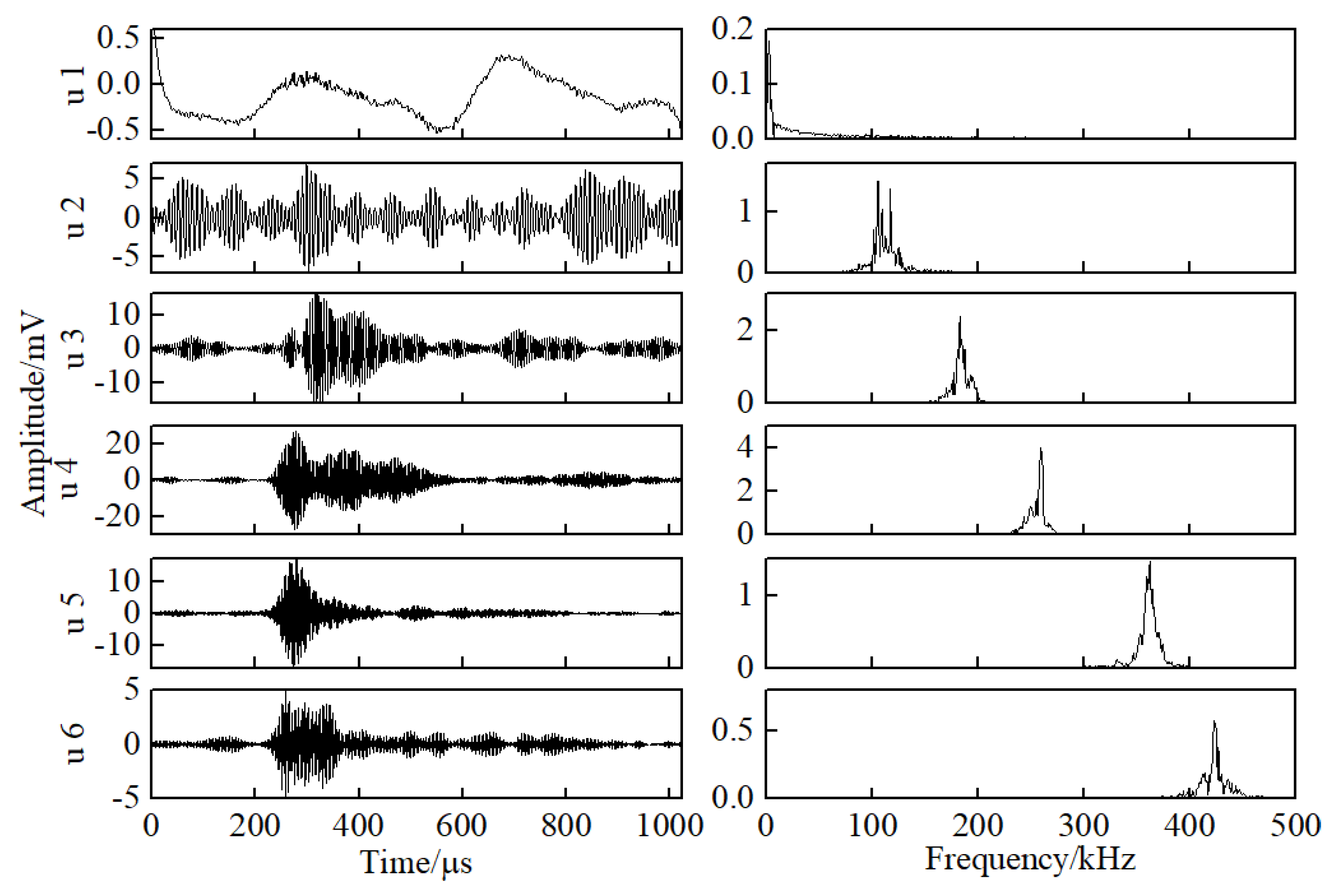
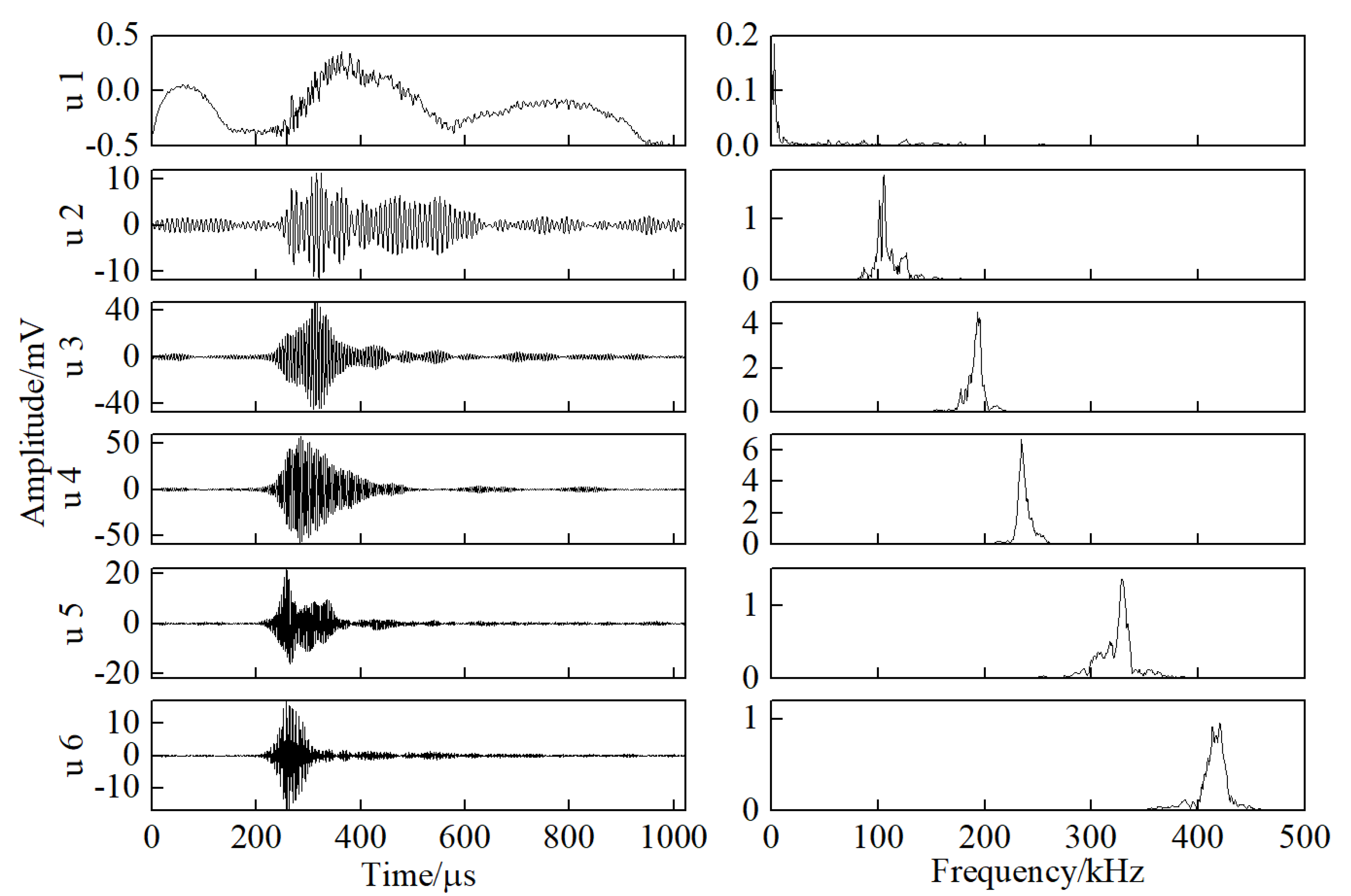
4.2. AE Signal Preprocessing Based on Variational Modal Decomposition

Based on the above analysis, the VMD was used to preprocess the AE signals collected at each stage. The VMD algorithm can obtain the optimal solution of the variational model by iterative optimization in the frequency domain, making it easy to determine the frequency center and bandwidth of each modal component [28].
There are two main purposes for VMD decomposing. The first one is to decompose the AE signal into two frequency bands, 50–200 kHz and 200–500 khz, ensuring no useful information was lost. The second purpose is to filter out the noise that has a frequency less than 50 kHz. Figure 6, Figure 7, Figure 8 and Figure 9 show the time- and frequency-domain plots of the various components of a typical AE signal in the four stages after six-layer VMD. It can be seen that the first component, u1, of all signals had an upper-limit frequency of less than 50 kHz and a peak frequency of about 3 kHz. Its amplitude and energy were both low, indicating a typical noise and irregular behavior. Of the five remained components, u2 and u3 were distributed between 50–200 kHz and had the characteristics of continuous signals, while u4-u6 were between 200–500 kHz and showed obvious burst-type characteristics. By comparing the amplitudes of each component at four stages, it can be found that they are completely consistent with the results described in the previous section.

4.3. AE Signal Energy Ratio in Deformation Damage

Based on the AE signal analysis in four stages, each component obtained by the VMD was first reconstructed into two signals positioned, respectively, in 50–200 kHz and 200–500 kHz. Then, the energy ratio R between two signals was calculated with Equations (3) and (4), as shown in Figure 10.
From Figure 10, we can find an obvious dividing line of R = −0.5 for the four stages, which is represented by a black dashed solid line. In the elastic-yield stage (Figure 10a) of TC11 titanium alloy, the majority of the AE signal energy ratio was greater than −0.5. This was due to the simultaneous elastic and plastic deformation of the material at this stage. Shifting and dislocation activities were extremely active, resulting in a great number of AE signals with large proportion of Hus. Some signals showed R values of greater than 0.5. After the deformation, the specimen began to come to the strengthening stage (Figure 10b). The number of signals with R value greater than −0.5 decreased sharply, and nearly no signals with R value greater than 0.5 were generated. At the same time, a large number of signals with R values less than −0.5 were generated. Due to the crystal slip and dislocation freedom reduction, a large area of dislocation plugging occurred. This reduced the energy of the collected AE signal Hus from the deformation of the specimen, and the signals Hns from the friction and hydraulic systems began to dominate. At the necking stage of the specimen deformation (Figure 10c), the R value of most signals was less than −0.5, and the plastic deformation of the material at this stage lost its balance. The plastic deformation, except the necking zone stops and the dislocation congestion produced by the necking area, increased significantly, which resulted in the AE signals generated by the deformation of the piece being greatly reduced in both quantity and amplitude. During the fracture stage (Figure 10d), the R value began to show similar characteristics to that in the elastic-yield stage. This was because under the three-dimensional tensile force inside the necking region, the front edge of the dense dislocation group produced a large tensile stress and aggregated to the weak part to start small cracks. The gradual propagating of the macro cracks led to the complete fracture of the TC11. The occurrence of cracks caused the Hus to dominate, resulting in a much lager R value.
In order to clearly show the distribution characteristics of the AE signal energy ratio R at the four stages of specimen deformation, a normal distribution curve was plotted and shown in Figure 11. It can be seen that the R value was mainly distributed in the (−0.5, 0.5) during the elastic-yield stage. There were two peaks in the strengthening stage. Most of the signal R values were distributed between (−1.5, −0.5), and some were in (−0.5, 0.5). The R value of the necking stage was mainly distributed over (−1.5, −0.5). The R values at the fracture stage were in (−0.5, 0.5). Table 5 shows the mean and standard deviation of the AE signal energy ratio of the four specimens in the tensile test.
In traditional approaches, the energy of the AE signal is one of the significant characteristic parameters. In order to show the advantage of the AE signal energy ratio R, the change of the AE signal energy with time was plot in Figure 11. The AE energy gradually decreased with the progress of deforming, but the change did not apparently show the stage-related features. We can only make a rough assessment of the state of the specimen using this parameter, and it is hard to determine the deformation stage. However, the calculated AE signal-to-energy ratio exhibited direct phase characteristics. According to the distribution of R value, the deformation stage of the specimen can be judged effectively. Thus, as the blade enters the dangerous necking stage, the crack can be well predicted by signal energy ratio, so that the blade can be repaired or replaced before an accident happens.

4.4. AE Crack Initiation Identification Method

From Figure 5 to Figure 9, we observed that the AE signal in the fracture stage had obvious sudden signal characteristics, with two peak frequencies located between 150–200 kHz and 200–250 kHz. In Figure 9, the signals in these frequency ranges originated from the beginning of the AE activity, eliminating the possibility of these high-frequency signals being related to wave reflection. For the remaining three stages of deformation, there were stable signal components within 50–150 kHz. These signals were mainly generated from the friction between the specimen and the fixture and the hydraulic system of the testing machine.
Based on the analysis results of the time- and frequency-domain of the AE signals, two Partial Energies (PE), PE1 and PE2, were employed, corresponding to the signal energy with frequency positioned in the range of 50–150 kHz and 150–500 kHz, respectively. The VMD was used to decompose the signal in 10 layers. The ith component obtained by the decomposition was recorded as ui, and the Peak Frequency (PF) corresponding to each component was recorded as pfi. For each AE signal, the values of PE1 and PE2 were:
PE 1 = i = 1 n 1 E ( u i ) p f i [ 50 , 150 ] kHz PE 2 = i = 1 n 2 E ( u i ) p f i [ 150 , 500 ] kHz
where E ( u i ) is the energy ratio between the ui component and the total energy of the signal.
From Figure 5, by comparing the signal in the elastic-yield stage to the signal peaks in the fracture stage, we found that there was no significant difference of signal peaks between 150–300 kHz at the fracture stage. In order to distinguish the AE signals between these two stages, a AE characteristic parameter, Weighted Peak Frequency (WPF), is presented, which is expressed by:
WPF = { i = 1 n 1 E ( u i ) p f i PE 1 PE 1 > PE 2 i = 1 n 2 E ( u i ) p f i PE 2 PE 1 PE 2 ,
We found that the calculated Weighted Peak Frequency can distinguish the AE signals dominated by PE1 and PE2, respectively. Additionally, for all the AE signals dominated by PE2, the different energy distribution characteristics can be displayed in the frequency of greater than 150 kHz. Thus, the AE signal generated after the crack initiation can be identified from the elastic yield stage.
In every stage of deformation damage, 200 AE signals were selected (uniformly distributed in the time history) for each stage of TC11 titanium alloy deformation. The PE2 values of the decomposed 800 AE signals for the four stages were plotted in a two-dimensional scatter diagram as shown in Figure 12, with the WPF being the abscissa. We can see that the AE signal after the crack was clearly distinguished, and it was mainly concentrated in the range of PE2 > 0.7 and WPF < 235 kHz. For the signals of PE2 < 0.5 and WPF < 150 kHz, these ranges were mainly related to the AE signals generated by the friction and hydraulic systems with low signal-to-noise ratio. The AE signal in the elastic-yield stage was mainly distributed in the range of PE2 > 0.7 and WPF > 235 kHz. Therefore, the combination of PE2 and WPF can effectively identify the crack initiation during the tensile process of the specimen. In the fracture stage, 8 out of the 200 signals fell outside the crack initiation area, but these points did not lead to a misjudgment of the result. We also found that there were 22 out of the 600 signals in the remaining three stages which fell in the crack initiation area. These 22 points gave us a small percent error. Therefore, the correct rate of judgment on the crack is 96.33%, which was calculated with the presented two parameters. We should also notice that using this method caused the crack initiation time showed to be earlier than the macroscopic crack time recorded by the micro camera.

5. Conclusions

In this study, the AE was used to monitor the deformation and damage of TC11 titanium alloy specimens. A characteristic parameter of AE signal energy ratio was used to determine the deforming stage of the specimen. The VMD was used to decompose the AE signals into different frequency ranges. The result showed that the AE signal energy ratio had a better performance compared with the traditional AE energy indicator. In addition, a method combining the partial energy ratio (PER) and the weighted peak frequency (WPF) was employed to determine the crack occurrence. The following conclusions can be drawn:
  • The AE signals collected in the four stages of blade deformation had different characteristics in the time domain or the frequency domain. Thus, the AE can be used to obtain the deformation state of the specimen in time.
  • Preprocessing the AE signal by the VMD method can effectively filter out noises with frequencies less than 50 kHz, and it can decompose the AE signal in the frequency domain.
  • The AE signal energy ratio, the ratio of the AE signal energy generated by deformation to the signal energy generated by friction and hydraulic systems, can be used to identify the deformation stage of the test specimen, showing better robustness than the traditional AE characteristic parameters.
  • The combined use of the PER and WPF of the AE signal can determine the time of crack occurrence in the TC11 titanium alloy material, but with an earlier prediction time than the actual observation from the micro camera device.
  • The method we proposed in the paper will help to eliminate the need for a middle sensor by separating the noise based on frequency.

Author Contributions

J.H. conceived and designed the experiments; J.H. and Z.Z. performed the experiments under the supervision of G.Y.; J.H., Z.Z. and C.H. analyzed the data under the supervision of G.Y.; G.Y. contributed reagents/materials/analysis tools; J.H. wrote the paper under the supervision of G.Y. All authors have read and agreed to the published version of the manuscript.

Funding

This work is partially supported by the National Natural Science Foundation of China (Grant No. 51575035).

Conflicts of Interest

The authors declare no conflict of interest.

References

  1. Hamed, A.; Tabakoff, W.C.; Wenglarz, R.V. Erosion and Deposition in Turbomachinery. J. Propuls. Power 2012, 22, 350–360. [Google Scholar] [CrossRef] [Green Version]
  2. Witek, L. Experimental crack propagation and failure analysis of the first stage compressor blade subjected to vibration. Eng. Fail. Anal. 2009, 16, 2163–2170. [Google Scholar] [CrossRef]
  3. Silveira, E.; Atxaga, G.; Irisarri, A.M. Failure analysis of a set of compressor blades. Eng. Fail. Anal. 2008, 15, 666–674. [Google Scholar] [CrossRef]
  4. Mishra, R.K.; Srivastav, D.K.; Srinivasan, K.; Nandi, V.; Bhat, R.R. Impact of Foreign Object Damage on an Aero Gas Turbine Engine. J. Fail. Anal. Prev. 2015, 15, 25–32. [Google Scholar] [CrossRef]
  5. Quan, Y.M.; Xu, H.; Ke, Z.Y. Research on some influence factors in high temperature measurement of metal with thermal infrared imager. Phys. Procedia 2011, 19, 207–213. [Google Scholar]
  6. Papakyriacou, M.; Mayer, H.; Fuchs, U.; Stanzl-Tschegg, S.E.; Wei, R.P. Influence of atmospheric moisture on slow fatigue crack growth at ultrasonic frequency in aluminium and magnesium alloys. Fatigue Fract. Eng. Mater. Struct. 2010, 25, 795–804. [Google Scholar] [CrossRef]
  7. Szczepankowski, A.; Szymczak, J. Initiation of Damage to the Hot Part of Aircraft Turbine Engines. Res. Work. Air Force Inst. Technol. 2016, 38, 61–74. [Google Scholar] [CrossRef] [Green Version]
  8. García, I.; Zubia, J.; Durana, G.; Aldabaldetreku, G.; Illarramendi, M.A.; Villatoro, J. Optical Fiber Sensors for Aircraft Structural Health Monitoring. Sensors 2015, 15, 15494–15519. [Google Scholar] [CrossRef] [Green Version]
  9. Mukhopadhyay, S.C.; Ihara, I. Sensors and Technologies for Structural Health Monitoring: A Review. In New Developments in Sensing Technology for Structural Health Monitoring; Springer Berlin and Heidelberg GmbH & Co. KG: Berlin, Germany, 2011; pp. 78–82. [Google Scholar]
  10. Barile, C.; Casavola, C.; Pappalettera, G.; Vimalathithan, P.K. Damage characterization in composite materials using acoustic emission signal-based and parameter-based data. Compos. Part B 2019, 178, 107469. [Google Scholar] [CrossRef]
  11. Beattie, A.G. Acoustic emission, principles and instrumentation. J. Acoust. Emiss. 1983, 2, 95–128. [Google Scholar]
  12. Ativitavas, N.; Fowler, T.; Pothisiri, T. Acoustic Emission Characteristics of Pultruded Fiber Reinforced Plastics under Uniaxial Tensile Stress; European Working Group on Acoustic Emission: Berlin, Germany, 2004; pp. 447–454. [Google Scholar]
  13. Barre, S.; Benzeggagh, M.-L. On the use of acoustic emission to investigate damage mechanisms in glass-fiber reinforced polypropylene. Compos. Sci. Technol. 1994, 52, 369–376. [Google Scholar] [CrossRef]
  14. Marec, A.; Thomas, J.H.; Guerjouma, R.E. Damage characterization of polymer-based composite materials: Multivariable analysis and wavelet transform for clustering acoustic emission data. Mech. Syst. Signal Process. 2008, 22, 1441–1464. [Google Scholar] [CrossRef]
  15. Jiang, J.; Ye, C.; Zhang, Z.Z.; Zhang, B.B. Study on Sources Classification Amplitude Criterion of Non-ferrous Metal Pressure Vessel Acoustic Emission Inspection. Petro-Chem. Equip. 2015, 44, 11–15. [Google Scholar]
  16. Maire, E.; Carmona, V.; Courbon, J.; Ludwig, W. Fast X-ray tomography and acoustic emission study of damage in metals during continuous tensile tests. Acta Mater. 2007, 55, 6806–6815. [Google Scholar] [CrossRef]
  17. Hu, S.W.; Lu, J.; Fan, X.Q. The Fracture of Concrete Based on Acoustic Emission. Appl. Mech. Mater. 2011, 80–81, 261–265. [Google Scholar] [CrossRef]
  18. Elforjani, M.A. Condition Monitoring of Slow Speed Rotating Machinery Using Acoustic Emission Technology. Ph.D. Thesis, Cranfield University, Cranfield, UK, 2010. [Google Scholar]
  19. Harris, D.O.; Dunegan, H.L. Continuous monitoring of fatigue-crack growth by acoustic-emission techniques. Exp. Mech. 1974, 14, 71–81. [Google Scholar] [CrossRef]
  20. Haugse, E.D.; Leeks, T.J.; Ikegami, R.; Johnson, P.E.; Ziola, S.M.; Dorighi, J.F.; May, S.; Phelps, N. Crack growth detection and monitoring using broadband acoustic emission techniques. In Nondestructive Evaluation of Aging Aircraft, Airports, and Aerospace Hardware III; Proc. SPIE: Newport Beach, CA, USA, 1999. [Google Scholar]
  21. Blanchette, Y.; Dickson, J.I.; Bassim, M.N. Acoustic emission behavior during crack growth of 7075-T651 Al alloy. Eng. Fract. Mech. 1986, 24, 647–656. [Google Scholar] [CrossRef]
  22. Merson, D.L.; Razuvaev, A.A.; Vinogradov, A.Y. Application of the Spectral Analysis of Acoustic Emission Signals to Studies of Vulnerability of TiN Coatings on Steel Substrates. Russ. J. Nondestruct. Test. 2002, 38, 508–516. [Google Scholar] [CrossRef]
  23. Świt, G.; Adamczak, A.; Krampikowska, A. Time-frequency analysis of acoustic emission signals generated by the Glass Fibre Reinforced Polymer Composites during the tensile test. Mater. Sci. Eng. Conf. Ser. 2017, 251, 012002. [Google Scholar] [CrossRef]
  24. Lu, C.; Ding, P.; Chen, Z. Time-frequency Analysis of Acoustic Emission Signals Generated by Tension Damage in CFRP. Procedia Eng. 2011, 23, 210–215. [Google Scholar] [CrossRef] [Green Version]
  25. Rocadenbosch, F.; Soriano, C.; Comerón, A.; Baldasano, J.M. Lidar Inversion of Atmospheric Backscatter and Extinction-To-Backscatter Ratios by Use of a Kalman Filter. Appl. Opt. 1999, 38, 3175–3189. [Google Scholar] [CrossRef] [PubMed] [Green Version]
  26. Barely Visible Impact Damage Assessment in Laminated Composites Using Acoustic Emission. Available online: https://www.researchgate.net/publication/326333149 (accessed on 14 July 2018).
  27. Huang, N.E.; Shen, Z.; Long, S.R.; Wu, M.C.; Shih, H.H.; Zheng, Q.; Yen, N.C.; Tung, C.C.; Liu, H.H. The empirical mode decomposition and the Hilbert spectrum for nonlinear and non-stationary time series analysis. Proc. R. Soc. Lond. 1998, 454, 903–955. [Google Scholar] [CrossRef]
  28. Dragomiretskiy, K.; Zosso, D. Variational mode decomposition. IEEE Trans. Signal Process. 2014, 62, 531–544. [Google Scholar] [CrossRef]
  29. Yin, A.; Ren, H. A propagating mode extraction algorithm for microwave waveguide using variational mode decomposition. Meas. Sci. Technol. 2015, 26, 095009. [Google Scholar] [CrossRef]
  30. Ono, K. Acoustic Emission in Materials Research—A Review. J. Acoust. Emiss. 2011, 29, 284–308. [Google Scholar]
  31. Sause, M. Identification of Failure Mechanisms in Hybrid Materials Utilizing Pattern Recognition Techniques Applied to Acoustic Emission Signals. Ph.D. Thesis, Augsburg University, Augsburg, Germany, 2010. [Google Scholar]
  32. Sherine, M.E.; Kumari, S.L. Study of acoustic emission signals in continuous monitoring. In Proceedings of the Circuit, Power and Computing Technologies (ICCPCT), Kollam, India, 20–21 April 2017. [Google Scholar]
  33. GB/T228.1-2010. Metallic Materials-Tensile Testing-Part 1: Method of Test at Room Temperature; Standardization Administration of the P. R. C., Standards Press of China: Beijing, China, 2011. [Google Scholar]
  34. ASTM E/E8M-13. Standard Test Methods for Tension Testing of Metallic Materials; ASTM International: West Conshohocken, PA, USA, 2013. [Google Scholar]
  35. Kundu, T.; Nakatani, H.; Takeda, N. Acoustic source localization in anisotropic plates. Ultrasonics 2012, 52, 740–746. [Google Scholar] [CrossRef]
  36. Maugis, D.; Pollock, H.M. Surface forces, deformation and adherence at metal microcontacts. Acta Metall. 1984, 32, 1323–1334. [Google Scholar] [CrossRef]
  37. Kuwabara, T.; Sugawara, F. Multiaxial tube expansion test method for measurement of sheet metal deformation behavior under biaxial tension for a large strain range. Int. J. Plast. 2013, 45, 103–118. [Google Scholar] [CrossRef]
  38. Botvina, L.R.; Tyutina, M.R.; Petersenb, T.B.; Levina, V.P.; Soldatenkova, A.P.; Prosvirnin, D.V. Residual Strength, Microhardness, and Acoustic Properties of Low-Carbon Steel after Cyclic Loading. J. Mach. Manuf. Reliab. 2018, 47, 516–524. [Google Scholar] [CrossRef]
  39. Botvina, L.R.; Shebalin, P.N.; Oparina, I.B. The mechanism of temporal variations of seismicity and acoustic emission before microfracture. Dokl. Akad. Nauk 2001, 376, 480–484. [Google Scholar]
  40. Botvina, L.R.; Tyutin, M.R. New acoustic parameter characterizing loading history effects. Eng. Fract. Mech. 2019, 210, 358–366. [Google Scholar] [CrossRef]
  41. Barile, C. Innovative Mechanical characterization of CFRP by using acoustic emission technique. Eng. Fract. Mech. 2019, 210, 414–421. [Google Scholar] [CrossRef]
  42. Fatih, L.O.; Nuri, E.; Stepan, V. Do high frequency acoustic emission events always represent fibre failure in CFRP laminates? Compos. Part A 2017, 103, 230–235. [Google Scholar]
Figure 1. Shape and size of TC11 titanium alloy tensile specimen (mm).
Applsci 10 03674 g001
Figure 2. Experimental test system and sensor layout.
Applsci 10 03674 g002
Figure 3. Amplitude of AE signals induced by stress of TC11.
Applsci 10 03674 g003
Figure 4. Crack observed by the micro camera.
Applsci 10 03674 g004
Figure 5. Typical time- (left column) and frequency-domain (right column) AE signals induced by the deformation of TC11 titanium alloys: (a) Elastic-yield section; (b) Strengthening section; (c) Necking section; (d) Fracture section.
Applsci 10 03674 g005
Figure 6. Time-and frequency-domain components of the typical AE signals after the Variable Mode Decomposition (VMD) in the elastic-yield stage.
Applsci 10 03674 g006
Figure 7. Time-and frequency-domain components of the typical AE signals after the VMD in the strengthening stage.
Applsci 10 03674 g007
Figure 8. Time- and frequency-domain components of the typical AE signals after the VMD in the necking stage.
Applsci 10 03674 g008
Figure 9. Time- and frequency-domain components of the typical AE signals after the VMD in the fracture stage.
Applsci 10 03674 g009
Figure 10. AE signal energy ratio of titanium alloy in four stages of deformation damage: (a) Elastic yield stage; (b) Strengthening stage; (c) Necking stage; (d) Fracture stage.
Applsci 10 03674 g010
Figure 11. Normal distribution curve of AE signal energy ratio in four stages of deformation damage of TC11 titanium alloy.
Applsci 10 03674 g011
Figure 12. PE2-WPF during deformation and damage of titanium alloy.
Applsci 10 03674 g012
Table 1. Alloy composition of TC11 titanium alloy.
Alloy CompositionAlMoZrSiTi
Quality score (%)5.8–7.02.8–3.80.8–2.00.20–0.35margin
Table 2. Tensile properties of TC11 titanium alloy bar (d = 20 mm).
Temperature θ/°C δ b / MPa δ p 0.2 / MPa δ 5 / % ψ / %
201114101417.652.1
50078059322.459.0
Note: 1. δ b is tensile strength, δ p 0.2 is yield strength, δ 5 is elongation after breaking and ψ is rate of reduction in area.
Table 3. AE system parameter settings.
Instrument ParametersValue
Sampling frequency/MHz1
Sampling length/k
Peak definition time/μs
Impact definition time/μs
Impact blocking time/μs
1 k
300
600
1000
Table 4. Details of Acoustic Emission (AE) sensors.
SensorResonant Frequency/kHzFrequency Range/kHzThreshold/dB
S1/S315050–40048
S2/S4650100–100038
Table 5. Mean and standard deviation of AE signal energy ratio in four stages of deformation of TC11.
Characteristic ValueSpecimenElastic-Yield StageStrengthening StageNecking StageFracture Stage
Mean value1
2
3
4
−0.084
−0.124
−0.076
−0.054
−0.145
−0.167
−0.092
−0.085
−0.973
−1.017
−0.954
−0.921
−0.974
−1.114
−0.967
−0.957
−0.196
−0.210
−0.185
−0.231
Standard deviation1
2
3
4
0.266
0.244
0.198
0.231
0.218
0.195
0.241
0.187
0.178
0.183
0.154
0.207
0.189
0.213
0.171
0.192
0.209
0.167
0.204
0.157

