Article

Assessment of the Future Climate Change Projections on Streamflow Hydrology and Water Availability over Upper Xijiang River Basin, China

1
College of Civil Engineering and Architecture, Guangxi University, Nanning 530004, China
2
Guangxi Key Laboratory of Disaster Prevention and Engineering Safety, Nanning 530004, China
3
Civil Engineering Department, University of Engineering and Technology, Peshawar 25000, Pakistan
4
Key Laboratory of Plant Genetic and Breeding, College of Agriculture, Guangxi University, Nanning 530004, China
5
School of Civil and Environmental Engineering (SCEE), National University of Sciences and Technology, Islamabad 44000, Pakistan
6
Environmental Protection Agency, Lahore 54000, Pakistan
*
Author to whom correspondence should be addressed.
Appl. Sci. 2020, 10(11), 3671; https://doi.org/10.3390/app10113671
Submission received: 15 April 2020 / Revised: 22 May 2020 / Accepted: 23 May 2020 / Published: 26 May 2020
(This article belongs to the Special Issue Hydrologic and Water Resources Investigations and Modeling)

Abstract

:
Hydrological models are widely applied for simulating complex watershed processes and directly linking meteorological, topographical, land-use, and geological conditions. In this study, the Soil and Water Assessment Tool (SWAT) was calibrated at two monitoring stations, which improved model performance and increased the reliability of flow predictions in the Upper Xijiang River Basin. This study evaluated the potential impacts of climate change on the streamflow and water yield of the Upper Xijiang River Basin using Arc-SWAT. The model was calibrated (1991–1997) and validated (1998–2001) using the Sequential Uncertainty Fitting Algorithm (SUFI-2). Model calibration and validation suggest a good match between the measured and simulated monthly streamflow, indicating the applicability of the model for future daily streamflow predictions. Large negative changes of low flows are projected under future climate scenarios, exhibiting a 10% and 30% decrease in water yield over the watershed on a monthly scale. Overall, findings generally indicated that winter flows are expected to be affected the most, with a maximum impact during the January–April period, followed by the wet monsoon season in the May–September period. Water balance components of the Upper Xijiang River Basin are expected to change significantly due to the projected climate change that, in turn, will seriously affect the water resources and streamflow patterns in the future. Thus, critical problems, such as ground water shortages, drops in agricultural crop yield, and increases in domestic water demand are expected at the Xijiang River Basin.

1. Introduction

Water is an essential element for the survival of life, economic growth, and development of the agricultural industry [1]. However, rapid population growth, urbanization, and industrialization have exerted unprecedented pressure over this limited resource. In addition to scarcity, the contamination of water resources is another chronic threat. To overcome future water stresses, the assessment of future trends and the availability of sustainable quantities of water resources at local to global scales has become inevitable [2]. Sustainable water resource management needs to analyze and quantify several hydrological processes taking place within the watershed [3]. Land-use and land-cover (LULC) changes affect these hydrological processes, so LULC practices and water resource management are closely related [4]. Unplanned LULC change remains a critical challenge for society, which seriously threatens the global environment and can result in severe impacts on human livelihood [5]. Anthropogenic effects have markedly modified global eco-systems. These rapid changes can be seen as the results of socio-economic development, population growth, and deforestation for the expansion of cities [6]. Anthropogenic forcing mainly includes the emissions of greenhouse gases (GHGs), as well as land-use/land-cover changes [7].
Climate change and land-use change have played a major role in building stress over the water resources of the La Boung River Basin in the south of Vietnam, where a significant decrease in number of wet days and annual streamflow has been found using the Soil and Water Assessment Tool (SWAT) model [8]. Evidence suggests that human activities have significantly imbalanced the hydrological cycle, resulting in the frequent occurrence of extreme events [9]. Flood risks due to distinct environmental changes and human activities have created huge concerns for climate change experts [10]. Frequent extreme precipitation events have caused severe floods, leading to runoff [11]. Global warming-altered precipitation and temperature patterns could have a significant impact on the local hydrological cycle [12]. Changes in the hydrological cycle result in the alteration of stream water flow patterns. Other factors that modify stream discharges are retardation of infiltration and evapotranspiration processes [13]. Changes in LULC were shown to decrease evapotranspiration losses, resulting in a 15% increase in water yield from 1994–2014 and a 40% increase is predicted during the period 2014–2029 in the upper Citarum watershed, Indonesia [14]. Future hydrological projections for the Upper Indus Basin have indicated high flows in spring and winter with low values of annual recurrence intervals, increasing the possibility of future flood hazards in the Upper Indus Basin [15].
Hydrological models have been widely used by researchers to evaluate the impact of climate change on the hydrological regimes. These tools help to quantify several hydrological parameters such as streamflow, run-off, evapotranspiration, and water yield. Computation of these hydrological parameters and selection of hydrological tools are critical in evaluating the present and future impacts of climate change [2,16]. Due to the wider application of the Soil and Water Assessment Tool (SWAT), it was selected to simulate the hydrological parameters under current and future climate at a basin-scale [17,18,19]. SWAT has already been successfully applied, at a basin-scale, to study water quality and water quantity under a wide range of environmental conditions around the globe. The main benefit of choosing SWAT is its modular implementation, where processes can be represented by parameters in the model and can be run with a minimum number of parameters [20,21]. Distributed hydrological models are associated with some degree of uncertainty, due to the poor quality of the input data and conceptual simplification of environmental processes [22,23]. The performance of the SWAT model to simulate the streamflow and water balance was reliable when calibrated with streamflow [24]. Yuan, Zhao [25] found that statistical downscaling (SD) is the most predominant uncertainty source in projections of extremely high flow and has a considerable contribution to the uncertainty in monthly streamflow over the Xijiang River Basin. Zhang, Lu [26] determined that changes in the discharge time series were identified by applying the Mann–Kendall test and Pettitt test for abrupt changes in the Pearl River Basin. They maintained that the annual water discharge had been significantly influenced by the precipitation variability and that the introduction of reservoirs at the Upper Xinjiang River Basin had little influence on water discharge. Unlike previous studies, Zhu, Das [27] compared a physically-based distributed model, Liuxihe (LXH), and a lumped conceptual model, Xinanjiang (XAJ), to assess the impact of climate change on streamflow using one global climate model BCC-CSM-1.1 under two future scenarios, representative concentration pathway (RCP)-4.5 and RCP-8.5, over the Xijiang River Basin. They found that the distributed model generated a high magnitude and correctly simulated higher peaks than the lumped model. Hydrological response to climate change in the Tarim Basin, China, under the mean conditions of four RCPs, showed a decrease of 21.5–40% in annual mean runoff [28]. Many studies have shown interest in analyzing the chain of uncertainties—from the general circulation models (GCMs) over all four emission scenarios (RCPs) to hydrological models—in order to improve the reality and robustness of future projections [28,29].
The Xijiang River Basin is the main tributary of the Pearl River Basin, which lies in the sub-tropical region of South China. The Pearl River Basin is the third largest river basin of China, serving the demands of more than 100 million people. Since 1990, the Xijiang River Basin observed frequent flooding disasters due to heavy storm events [30]. The Xijiang River Basin has not undergone rapid land-cover changes historically; however, government reforms in the early 1980s, which aimed to enhance the economic growth and improve the living standards in the area, yielded an urbanization rate of 300% and reflected notable impacts over the area’s hydro-climatology [31,32]. Ren, Zhou [33] presented evidence on the rapid urbanization effect. An increase in temperature of 0.05 °C per decade was recorded because of urbanization in mainland China. Many researchers have analyzed the impact of climate change on water resources in the Xijiang River Basin. However, to the best of our knowledge, no study has reported a comprehensive evaluation of the impacts of climate change on streamflow and water yield using several global climate models (GCMs) under all four future scenarios. Guo, Hu [34] summarized that the climate plays a key role in changing basin hydrology and streamflow in the Xijiang River Basin.
This study aimed to assess the effects of future climate change on streamflow and water yield over the Upper Xijiang River Basin. The Soil and Water Assessment Tool (SWAT) was used to simulate streamflow using global climate models (GCMs) under the future scenarios of all four representative concentration pathways (RCPs). The uncertainty in runoff projections related to GCMs and land use land cover (LULC) scenarios were also investigated. Finally, the projections in streamflow and water yield were revealed. This study was intended to serve as a contribution to the literature and to assist decision-makers, policy formulators, and so on.

2. Materials and Methods

The methodology was as follows: (1) Statistical downscaling of global climate models and bias-correction; (2) Hydrological modeling of the Upper Xijiang River Basin with multi-gauge calibration and validation; and (3) Analyzing streamflow and water yield under historical and future climate scenarios.

2.1. Study Area

The selected study area is the Upper Xijiang River Basin (Figure 1) upstream of the Qianjiang river gauge station, which is the largest river basin contributing to the Pearl River Basin located in South China. The total drainage area of the Upper Xijiang River Basin is 1.18 × 10⁵ km2.
The Xijiang River originates from the Maxiong mountains of Yunnan province in southwest China and flows southeastward, passing through Guizhou, Guangxi, and Guandong provinces, and flows into the South China Sea. The main channel of the Upper Xijiang River Basin has distinctive names for particular sections: Beipanjiang, Nanpanjiang, Hongshuihe, and Qianjiang [26]. The basin has a humid and tropical climate with ample precipitation and generally high air temperature. The mean air temperature varies from 14 to 22 °C. The mean annual precipitation remains between 1200 and 1900 mm. Precipitation mainly occurs from April to October, which accounts for 72–86% of the annual precipitation [35].

2.2. Input Data

2.2.1. Geo-Spatial Data

Hydrological modeling requires topographic data, soil characteristics, and land-use/land-cover (LULC) maps, as summarized in Table 1. The digital elevation model (DEM) is the most important data in the SWAT setup, providing topographic details. A shuttle radar topography mission digital elevation model (SRTM-DEM) with 90 m resolution (as delineated in Figure 2), obtained from the CGIAR Consortium for Spatial Information (CGIAR-CSI) (http://srtm.csi.cgiar.org/), was used. The DEM is the basic input layer in the model setup and is used to extract the slope and drainage network in the study area. The required soil map of the study area, the FAO–UNESCO global soil map (with 5 km resolution), was obtained from the Food and Agriculture Organization (FAO) (http://www.fao.org/nr/land/soils/digital-soil-map-of-the-world/en/).
Three LULC data types were obtained from various agencies to evaluate performance, presented in Table 1 and Figure 3. The Land-Cover Institute (LCI) of United States Geological Survey (USGS), based on 10 years (2001–2010) of collection, provided the 5.1 MCD12Q1 land-cover type data (with a resolution of 15 arc-seconds) (https://archive.usgs.gov/archive/sites/landcover.usgs.gov/global_climatology.html).
The LULC 2000 was obtained for the China region from the Global Land Cover 2000 map developed by Forest Resources and Carbon Emissions (IFORCE). (https://forobs.jrc.ec.europa.eu/products/glc2000/products.php).
LULC 1995, 2005, and 2015, developed by the European Space Agency (ESA) under the Climate Change Initiative CCI-LC project, were also analyzed to simulate streamflow and water yield. (http://maps.elie.ucl.ac.be/CCI/viewer/download.php).

2.2.2. Weather Data

Daily precipitation data from 36 weather stations and two stream gauge stations located in the Xijiang River Basin were obtained from the National Meteorological Information Centre (NMIC) of the Chinese Meteorological Administration (CMA).

2.2.3. Downscaling and Bias-Correction of Global Climate Model (GCM) Data

GCMs are important tools, which are preferable to understand climate change scenarios. These scenarios simulate the response of the global climate system to changes occurring in the atmospheric conditions [36]. Future monthly streamflow was simulated with five global climate models (GCMs) participating in the Coupled Model Inter-comparison Project Phase 5 (CMIP5) under four representative concentration pathways (RCPs) for the period of 2020–2050, considering the historical period of 1971–2001 for the baseline flow. Streamflow projections were carried out by assuming the projected precipitation and temperature inputs to SWAT, assuming non-evolution of the LULC ESA 2005 and soil properties in the future period. In this study, we analyze Geophysical Fluid Dynamics Laboratory, USA (GFDL-ESM2M), Meteorological Office Hadley Centre, United Kingdom (HadGEM2-ES), Institute Pieree Simon Laplace, France (IPSL-CM5A-LR), Atmospheric and Ocean Research Institute, The University of Tokyo, Japan (MIROC-ESM-CHEM), and Bjerknes Centre for Climate Research, Norwegian Meteorological Institute, Norway (NorESM1-M), of the Inter-Sectoral Impact Model Inter-comparison Project (ISI-MIP) [37], under the emission scenarios of all four representative concentration pathways (RCPs) (RCP-2.6, RCP-4.5, RCP-6.0, and RCP-8.5). The outputs of the GCMs were statistically downscaled using the bias-correction special disaggregation (BCSD) tool in the climate change toolkit (CCT) [38,39,40]. In detail, the climate change toolkit (CCT) extracted, downscaled, bias corrected, and interpolated the GCM outputs. All climate data sets (i.e., precipitation, temperature, relative humidity, solar radiation, and wind) were downscaled using a 0.5-degree spatial resolution and are available in simple text format. Projected changes in mean monthly streamflow were analyzed by the percent change method, yielding a percent increase or decrease. The historical GCM (1971–2001) was used as a baseline for future projection changes.

2.3. Soil and Water Assessment Tool (SWAT)

The Soil and Water Assessment Tool (SWAT) is a semi-distributed physically-based basin-scale model developed in [41]. Based on daily/sub-daily precipitation data, temperature, relative humidity, and wind speed data, the SWAT model uses the soil conservation services (SCS) method and simulates hydrological processes, such as surface runoff, snowmelt runoff, lateral flow, and infiltration in a river basin, as well as water balance and streamflow [42,43,44]. In the SWAT model, vegetation and soil characteristics are categorized by their hydrologic response unit (HRU). Run-off is calculated separately from the HRUs, and the total run-off of the entire catchment is calculated using the hydrological model [34]. The SWAT hydrological model is based on the basic water balance equation:
S W t = S W 0 + t = 1 t ( R d a y Q s u r f E a W s e e p Q g w ) ,
where S W t   ( mm   H 2 O ) is the final soil water content, S W 0   ( mm   H 2 O ) is the initial soil water, t is the time (in days), R day is the daily precipitation amount, Q surf is the surface run-off, E a is the actual evapotranspiration, W seep is the amount of water that percolates to the vadose zone on day t, and Q gw is the return flow on day t.
Water yield is one of the critical parameters for analyzing sustainable water resource management. The water yield is the cumulative amount of water leaving the HRU and entering the main tributary during a given time step [41,45]. Water yield within a basin is evaluated by the model based on the following equation:
W y i e l d = Q s + Q g w + Q l a t T l o s s ,
where W y i e l d is the measure of water yield (mm), Q s is the surface runoff (mm), Q g w is the groundwater flow (mm), Q l a t is the lateral flow contribution to the streamflow (mm), and T l o s s is the total losses (mm) from the tributary in the hydrologic response unit (HRU) by means of transmission through the bed. The water yield is one of the main components of water balance. The water balance is the (Precipitation = Water Yield + Evapotranspiration − Transmission Losses). Evapotranspiration is considered as the major loss. Water yield is the sum of surface runoff, groundwater flow, and lateral flow, subtracting transmission losses and pond abstractions. Total water yield (WYLD) is the amount of streamflow leaving the watershed outlet amid the time step. Surface runoff can be estimated using the Soil Conservation Service (SCS) curve number system by the United States Department of Agriculture (USDA), given by:
Q s = ( P d a i l y 0.2 S ) 2 ( P d a i l y + 0.8 S ) ,
S = 25.4 ( 100 C N 1 ) ,
where P d a i l y is the daily precipitation (mm), S (Equation (4)) is the retention parameter (mm), and C N is the curve number. The prediction of lateral flow by the SWAT model is defined as:
Q l a t = 0.024 ( 2 S S C sin α θ d L ) ,
where Q l a t is the lateral flow (mm/day), S is the drainable volume of soil water per unit area of saturated thickness (mm/day), S C is the saturated hydraulic conductivity (mm/hr), L is the flow length, sin α is the land slope, and θ d is the drainable porosity. The groundwater flow, Q g w , contributes to the main channel, which can be calculated as:
Q g w = Q g w 1 × e ω Δ t + W a q u ( 1 e ω Δ t ) ,
where Q g w is the groundwater flow (mm), ω is the baseflow recession constant, Δ t is the time step, and W a q u is the water recharge entering the aquifer (mm/day).

2.4. Model Calibration and Validation

The SWAT-CUP (Soil and Water Assessment Tool-Calibration and Uncertainty Program) software was developed to calibrate and validate hydrological processes by the SWAT model [23]. The Sequential Uncertainty Fitting Algorithm (SUFI-2), which is capable of analyzing a large number of parameters and measuring data from multi-gauge stations simultaneously, was used to obtain a better correlation between simulated and observed data, following [46]. Calibration is one of the processes that adjusts the model input parameter values and their boundary conditions to match the simulated values with the observed values [47]. Calibration can be carried out through uncertainty analysis (UA) or sensitivity analysis (SA), such that the model predictions lie within in a certain confidence range [48,49]. The applicability of the SWAT model can be checked through careful calibration using one of the following algorithms: generalized likelihood uncertainty estimation (GLUE), sequential uncertainty fitting (SUFI-2), parameter solution (ParaSol), and Markov chain Monte Carlo (MCMC) [46,50,51,52].
Modeled streamflow data were calibrated (1991–1997) and validated (1998–2001) with observed climatic data and five LULC scenarios for various time periods. Five performance indices were analyzed, and the results were satisfactory. Model calibration on a sub-stream scale was carried out. Finally, the calibrated parameters were used for the analysis in the Arc-SWAT project.
The objective functions, p-factor, and r-factor values for calibration (1991–1997) and validation (1998–2001) are presented in Table 2 and Table 3 with the observed precipitation and using various LULCs at Qianjiang and Tianr hydrological stations, respectively. The performance indicators of the model for Qianjiang station had more satisfactory results, compared to that for Tianr station. However, the performance indicator values for Tianr station, as shown in Table 3, still had acceptable values. These values confirmed the good performance of the model using observed climatic data and all five LULC scenarios.

2.4.1. SUFI-2 Algorithm

We calibrated and validated the SWAT model using the SUFI-2 algorithm, which considers several uncertainties in driving variables, measured data sets, conceptual data, and parameters [46]. A sensitivity analysis was carried out by using the Latin hypercube and one factor at a time (LH-OAT) sampling method in SWAT-CUP, where a set of model parameters was selected to identify the sensitive parameters that were capable of significantly affecting the model output [52,53]. In this study, 12 parameter sets were selected initially. Then, the model was run for 1000 iterations, on a monthly scale, at each gauge station during calibration and validation. Calibration and validation were performed using the observed and global climate model (historical) data sets with LULC, USGS (2001–2010), ESA (1995, 2005, 2015), and global land cover (GLC) China 2000. The p-value and t-state value were used to indicate the significance of sensitive parameters. A larger absolute t-stat and lower p-value (approaching zero) signifies higher sensitivity. The 95% percent prediction uncertainty (95PPU) was calculated through Latin hypercube sampling (LHS), which restricts 5% of the bad simulations. Further, the strength of the model calibration and validation was measured by the p-factor and r-factor, the values of which vary from 0 to 1. The p-factor indicates the measured data covered in a 95% range of uncertainty (95PPU). Highly sensitive parameters have lower p-factor values, where parameters with a near-zero p-factor are the most sensitive [54]. The r-factor is the average thickness of the 95PPU band divided by the standard deviation of measured data. A low r-factor describes less uncertainty and that approaching 1 indicates high uncertainty in a certain parameter [23]. SUFI-2 operates by performing several iterations. In each iteration, the parameter ranges get smaller, zooming in on the region of parameter space that produces better results than the previous iteration.

2.4.2. Statistical Performance Indices

This study used five objective functions—coefficient of regression (R2), Nash–Sutcliffe efficiency (NSE), percent bias (PBIAS), Kling–Gupta equation (KGE), and the ratio of root mean square error to standard deviation (RSR)—to evaluate the statistical performance of the SWAT model. R2 is the measurement of correlation between simulated and observed values, which is known as the coefficient of determination. The range of R2 varies from 0 to 1, where a value approaching 1 means better performance. The Nash–Sutcliffe equation (NSE) is a normalized, dimensionless statistic that defines the relative magnitude of residual variance, compared to the measured data variance [55]. The NSE value ranges from −∞ to 1, with an optimal value of 1 [56]. The KGE is the Kling–Gupta efficiency between observed and simulated values, with the treatment of missing values. This goodness of fit was developed in [57] to provide a decomposition of the NSE that facilitates the analysis of relative importance, such as correlation, bias, and variability, in the context of hydrological modeling. PBIAS (percent bias) calculates the average tendency of simulated values to be larger or smaller than the observed values [56]. A smaller magnitude of PBIAS indicates better model performance with an optimal value of zero. A positive PBIAS value indicates underestimation of the model, while negative values represent overestimation. RSR is the ratio of the root mean square error (RMSE) to the standard deviation. The values of the RSR range from 0 to ∞, where a lower RSR value indicates a lower RMSE value and a better model simulation performance [58]. A threshold of 0.5 is satisfactory for R2 and NSE [59]. The P-factor and R-factor were also used to evaluate model performance. A P-factor close to 1 and R-factor close to zero indicates a good fit. The P-factor is the percentage of measured data covered by 95PPU, while the R-factor is the ratio of the average of the band to the measurement of the standard deviation of measured variables, which varies from 0 to infinity; an R-factor value less than 1 indicates better performance [23]. A threshold for passing the sensitivity check (p-value < 0.05) could play a significant role in hydrological simulations [60].
The statistical performance parameters of the five global climate models (historical rainfall data), compared with the observed rainfall data, are shown in Table 4.

3. Results

3.1. Sensitivity Analysis (SA)

The sensitivity analysis performed to understand the processes and their associated parameters in SWAT were primarily controlling the hydrology of the watershed, particularly with respect to flow at the outlet. Based on the sensitivity analysis, the parameters soil evaporation and compensation factor (ESCO), runoff curve number (CN2), available soil water capacity (SOL_AWC), baseflow recession constant (ALPHA_BF), groundwater “revap” coefficient (GW_REWAP), Manning’s “n” value for overland flow (OV_N), depth from soil surface to bottom layer (SOL_Z), saturated hydraulic conductivity (SOL_K), groundwater delay time (GW_DELAY), and deep aquifer percolation fraction (RCHRG_DP) were identified as the most sensitive, as presented in Table 5.

3.2. Evaluation of LULC and Its Impacts on Streamflow

The results of monthly runoff calibration and validation for various LULC scenarios at Qianjiang and Tianr are presented in Figure 4 and Figure 5, respectively. Results achieved using LULC 1995 were a bit overestimated, while those using LULC GLC 2000 developed by IFORCE were slightly underestimated. The underestimation with GLC 2000 is shown in the LULC area classification in Table 6. The classified LULC had no urban area and a significant reduction in evergreen forest and increase in the deciduous forest area. Mixed forests dominated the basin, with a share of more than 60%. The urban land area increased from 0.146% in 1995 to 0.587% in 2015. The change in urban land, which is one of the major driving forces for changing runoff, was not significant. LULC (2001–2010) developed by USGS, showed that the map area was influenced mostly by mixed forests (68.425%) and slightly by urban land (0.982%).
The average observed streamflow at Qianjiang station was 2238.27 m3/s. The simulated average streamflow value was 2033.57 m3/s (9% decrease) with LULC (2001–2010) USGS; with LULC ESA (1995), it was 2521.11 m3/s (12% increase); with LULC ESA (2005), it was 2146.18 m3/s (4% decrease); with LULC ESA (2015), it was 2083.9 m3/s (6.89% decrease); and, with LULC GLC (2000), it was 1744.037 m3/s (22.08% decrease). The average observed streamflow at Tianr hydrological station was 1512.62 m3/s. The simulated average streamflow values were 1314.37m3/s (13.10% decrease) with LULC (2001–2010) USGS, 1721.55 m3/s (13.8% increase) with LULC ESA (1995), 1434.33 m3/s (5.17% decrease) with LULC ESA (2005), 1410.56 m3/s (6.74% decrease) with LULC ESA (2015), and 1312.33 m3/s (13.24% decrease) with LULC GLC (2000). LULC ESA (2005) and LULC USGS (2001–2010) showed the best match with the observed values. LULC ESA (2005) was, therefore, considered as a reference scenario for future streamflow projections based on the best match as well as the most acceptable parameter indices.

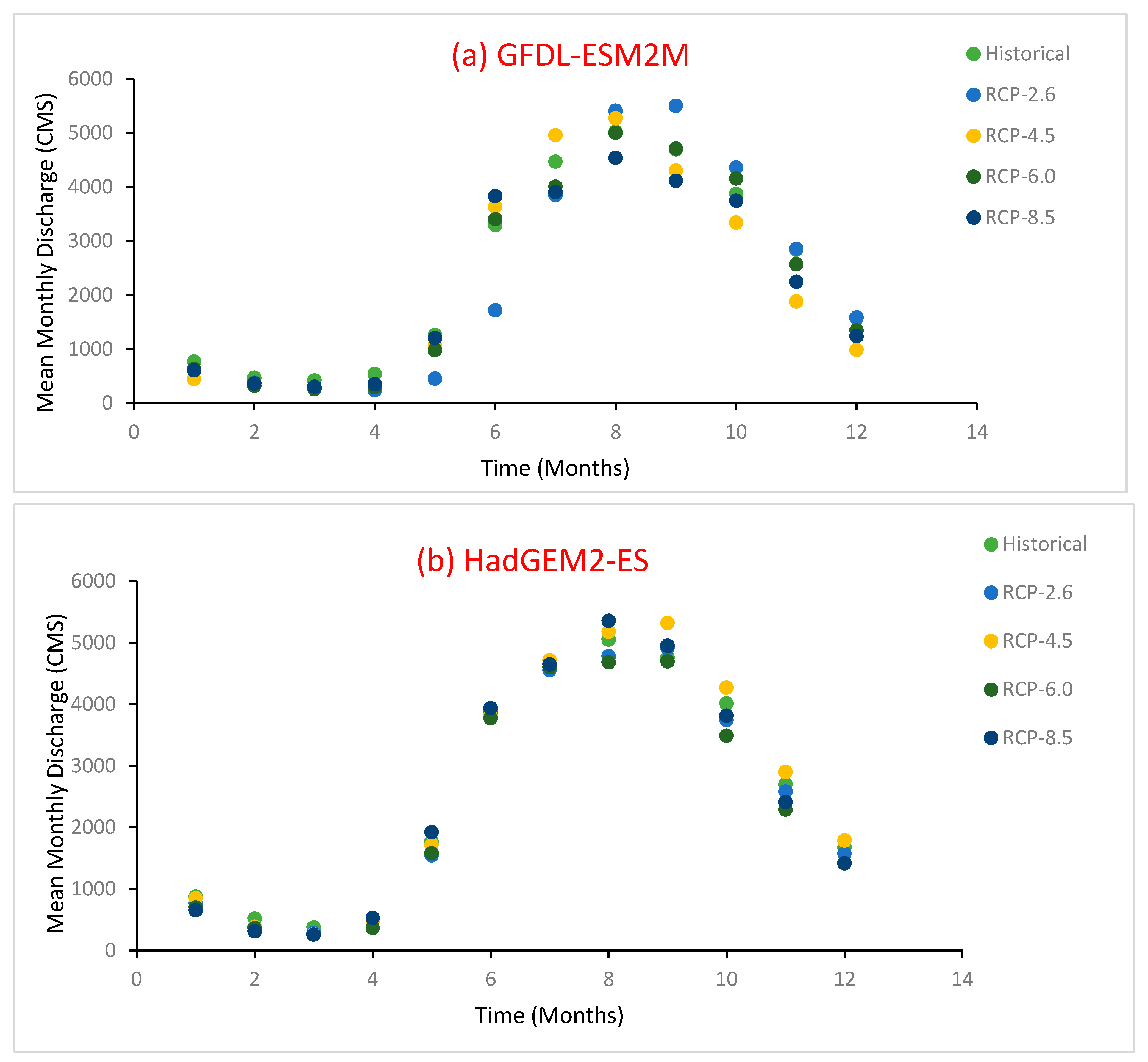
3.3. Future Projections of Mean Monthly Streamflow

The mean monthly streamflow for the historical period and future period under all four emission scenarios of each climate model are presented in Figure 6a–e. Future flow projections were compared for the basin outlet. The observed mean monthly discharge at Qianjiang hydrological station (considered as the basin outlet) was 2238.27 m3/s. The GFDL-ESM2M historical mean monthly discharge, presented in Figure 6a, was 2433.94 m3/s, while the projected mean monthly discharge under RCP-2.6 was 2267.93 m3/s; for RCP-4.5, 2231.61 m3/s; for RCP-6.0, 2306.45 m3/s; and for RCP-8.5, 2203.219 m3/s. The HadGEM2-ES historical mean monthly discharge, presented in Figure 6b, was 2560.865 m3/s, while the projected mean monthly discharge for RCP-2.6 was 2458.32 m3/s; for RCP-4.5, 2639.80 m3/s; for RCP-6.0, 2350.47 m3/s; and for RCP-8.5, 2516.08 m3/s. The IPSL-CM5A-LR historical mean monthly discharge, presented in Figure 6c, was 2546.93 m3/s, while the projected mean monthly discharge for RCP-2.6 was 2172.80 m3/s; for RCP-4.5, 2204.61 m3/s; for RCP-6.0, 2268.96 m3/s; and for RCP-8.5, 1911.05 m3/s. The MIROC-ESM-CHEM historical mean monthly discharge, presented in Figure 6d, was 2574.14 m3/s, while the projected mean monthly discharge for RCP-2.6 was 2268.74 m3/s; for RCP-4.5, 2250.32 m3/s; for RCP-6.0, 2355.68 m3/s; and for RCP-8.5, 2241.57 m3/s. The NorESM1-M historical mean monthly discharge, presented in Figure 6e, was 2546.93 m3/s, while the projected mean monthly discharge for RCP-2.6 was 2791.36 m3/s; for RCP-4.5, 2725.03 m3/s; for RCP-6.0, 2635.87 m3/s; and for RCP-8.5, 2692.98 m3/s. The five global climate models had similar patterns in pre-monsoon discharge trends, followed by abrupt peaks during monsoon and medium peaks post-monsoon. February, March, and April had the lowest peaks (i.e., lower than 1000 cm3/s).

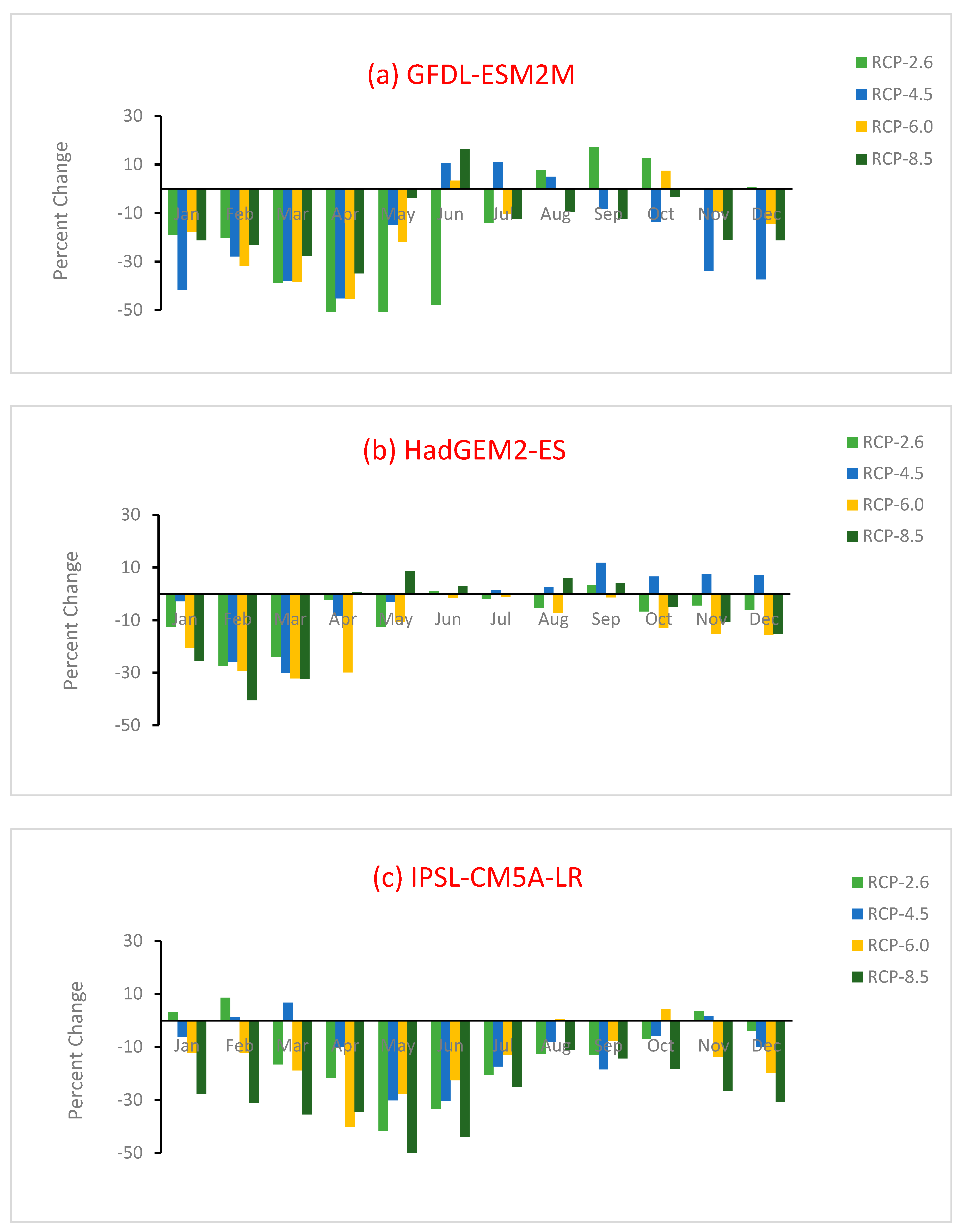
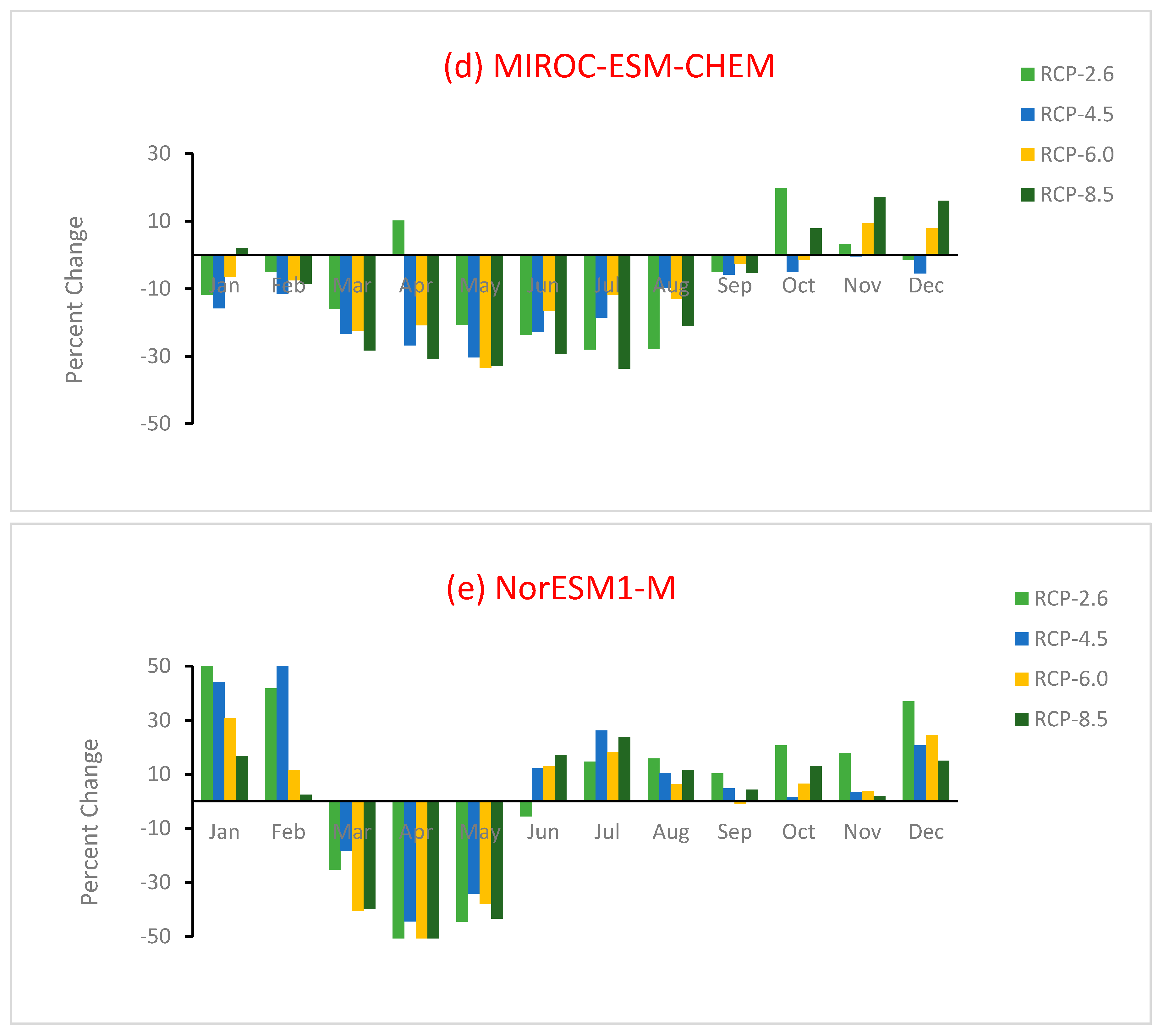
3.4. Projected Changes in Mean Monthly Streamflow

A significantly negative change was observed in all five GCMs. NorESM1-M had exceptional results, as shown in Figure 7e, showing a positive change during monsoon.
The effects of climate change on streamflow in the upper Xijiang River Basin at the Qianjiang outlet were estimated, as shown in Table 7. GFDL-ESM2M simulated negative change under all four scenarios, with a high chance (−19.5%) under RCP-4.5. HadGEM2-ES showed an unlikely slightly negative change (2.8%) under the same scenario. Only NorESM1-M showed a positive change (7.6% and 6.46% under RCP-2.6 and RCP-4.5, respectively). Summarizing the results, RCP-2.6 will likely decrease the streamflow by 7%, RCP-4.5 by 8.2%, RCP-6.0 by 11.4%, and RCP-8.5 by 13.5%. The average percent change of future scenarios predicts that the future streamflow will decrease by 8.1% under RCP-2.6, 8.2% under RCP-4.5, 11.45% under RCP-6.0, and 13.5% under RCP-8.5.
Similarly, the season-wise impacts of climate change on streamflow were also evaluated. The effect will likely be largest in the winter season, due to the cold temperature. The change in streamflow in the January–April period is higher, as compared to the wet-season of May–September. The dry climate corresponded to a decrease in streamflow. The largest decrease was observed in the January–April period, likely due to the declining trend of precipitation in this period.

3.5. Water Yield (WYLD) Response to Changing Climate under Future Scenarios

We also considered water yield, an important parameter estimated by the SWAT model for efficient water management and planning in watersheds. The contribution of each sub-basin in the watershed to the total water yield was analyzed for the observed data. The average annual basin values for the different water balance components during the calibration and validation periods simulated by the SWAT model are presented in Table 8. Evapotranspiration and groundwater contributed larger amounts to the water balance components. About 23% of the precipitation that occurs in the basin is returned to the atmosphere, when using evapotranspiration as a relative percentage of the average rainfall.
Total water yield (WYLD) is the amount of streamflow leaving the watershed outlet during the time step. The total annual water yield for 1991–2001 was predicted to be 1310.86 mm, comprising 58.55 mm of surface runoff, 1211.45 mm of baseflow (groundwater flow + tile flow), and 13.50 mm of lateral flow; the rest are transmission losses. Water yield for each year from 1991–2001 was quantified, as reported in Figure 8. Observed medium floods in 1994 and 1998 in Hongshui river, a tributary to the Xijiang River Basin, generated a large water yield, as also concluded by [61,62]. The lowest water yield was 82 mm in 1991, while a high value of water yield (1662 mm) was generated in 1998.
The results of the simulated mean annual water budget components for the Upper Xijiang River Basin under mean historical and future scenarios of five global climate models (GCMs) are presented in Table 9. The results also present the impacts of likely future climate change on the hydrologic conditions. The results are significant, especially in terms of evapotranspiration and water yield (WYLD). Evapotranspiration is increased by less than 5% under all future scenarios, compared to the baseline period.
Water yield is the most significant component of the water budget for sustainable water resource management and decision-making processes. Water yield for the future period (2020–2050) is summarized in Figure 9, while Figure 10 shows the percent change in water yield under baseline and future scenarios. There will be a likely decrease of 30% in water yield under the average of the future scenarios. A decrease of 40% is more likely under RCP-4.5. Figure 10 indicates that 2032, 2040, and 2049 will likely face substantial changes in water yield; while 2029, 2041, and 2042 will likely face slight changes in water yield.

3.6. Limitations

In this study, we did not consider the influence of reservoirs and other water storage options, which is the main limitation of this study. The authors of [26] studied long-term changes in annual water discharge and found that it is mainly controlled by precipitation variation. However, the construction of reservoirs/dams has had little influence on water discharge in the Zhujiang River Basin. The authors of [63] concluded that the impact of reservoirs should be considered in simulation of runoff. The projections of the SWAT model of hydrological components for the future scenarios were based on the use of the same LULC and soil properties as exist at present (LULC ESA-2005, in this study). This assumption may have led to underestimation of the actual evapotranspiration in the future periods [23]. Some hydropower and irrigation projects exist, which were also not included in this study, which may have altered the hydrology of the study area. Therefore, considering these limitations in the current research work, they should be accounted for in the projected results for the future planning of water resources.

4. Discussion

Quantification of uncertainty using the SUFI-2 algorithm showed that the largest share of uncertainty was related to the curve number, CN, as well as the soil properties for monthly streamflow and water yield projections during most of the annual cycle in the Upper Xijiang River Basin. This uncertainty mainly arose from the statistical downscaling, as well as the use of global LULC and soil data combined at a regional scale. These findings are in general agreement with most previous studies, which concluded that the LULC classification scheme and the validation methodology had the highest error contribution and implementation priority and showed that there are many inconsistencies between the definition of the map classes [64,65,66,67]. Kay, Davies [68] pointed out that the sensitivity of hydrological projections is based on the selection of global climate models (GCMs). The main objective of this study was to evaluate the best-suited representative land-use and climate change scenario for deducing the impacts on streamflow and water yield over the Upper Xijiang River Basin using the SWAT model. The most effective parameters for surface runoff calibration and validation, as categorized by Arnold, Moriasi [41] based on the behaviors of 64 watersheds, are CN2, AWC, ESCO, EPCO, OV_N, and SURLAG. The SWAT model was calibrated over the Pearl River Basin to evaluate the effects of temperature change on water discharge, where it was found that CN2, ESCO, RCHRG_DP, and SOL_AWC were the most sensitive parameters [69]. Memarian, Balasundram [70] highlighted the impacts of land-use and -cover change (LUCC) on the hydrological conditions (water discharge and sediment load) of a tropical basin were investigated by using the Soil and Water Assessment Tool (SWAT), where the most sensitive parameters were found to be RCHRG_DP, CN2, SOL_K, and SOL_AWC. The curve number, CN2, depends on soil and LULC characteristics and was found to be the most sensitive parameter, followed by SOL_AWC, ESCO, and SOL_K, in a study over the Eastern Nile Basin [71].
The main limitation of the SWAT model is that the baseflow simulation cannot generate acceptable values, as indicated by several studies [72,73]. In this study, we also concluded that parameters such as ground flow, tile flow, sublimation, and other related parameters are not well-simulated, resulting in sensitivity of the ESCO and ALPHA_BF parameters.
Uncertainty analysis (UA) is one of the techniques used to parameterize a hydrologic model and to reduce the uncertainty range [74]. The performance indices R2 and NSE were used to assess the goodness of fit between the observed and simulated values [72]. A hydrologic model can be assessed by multiple statistical and graphical performance indices, to compensate for the shortcomings of every performance indicator [75]. PBIAS, KGE, and RSR can be used to highlight poor model performance and integrate the benefits of an error index [58,76,77]. In this study, we achieved acceptable values for the five performance indicators reported in Table 10 (i.e., R2, NSE, PBIAS, KGE, and RSR).
The result of calibration and validation for both hydrological stations shows that the parameter indices are satisfactory; several studies have concluded that such values are acceptable in this range [2,78,79].
Land use and land cover (LULC) have been changing, either directly or indirectly, due to human activities. These changes affect the hydrological cycle and water balance components. In this study, LULC data from 1995, 2000, 2005, and 2015 developed by European Space Agency (ESA), USGS, and GLC IFORCE were evaluated to study the impacts on discharge and water yield. Awotwi, Yeboah [80] estimated a significant decrease in land cover, decline in surface water and base flow, and effects on annual water yield and evapotranspiration (ET). Woldesenbet, Elagib [81] found that an increase in surface run-off and decrease in baseflow and actual evapotranspiration would have negative impacts on water resources. In this study, we revealed that simulated values for all LULC scenarios showed a decrease in surface runoff and increase in baseflow. Global climate models’ (GCMs’) data simulated by the SWAT model for both historical (1971–2001) and future (2020–2050) periods reported that an increase in evapotranspiration will likely decrease surface runoff and base flow, with a resulting decrease in water yield under future RCP scenarios. Similar results were reported in Yom and Nan River Basins, Thailand. Moreover, these quantitative changes will be a challenge and will be more sever in the near future and can directly impact water availability [82].
This study has improved our understanding of the relationship between climate-induced changes and LULC changes on streamflow regime indicators that are relevant for the well-being of humans and freshwater ecosystems. Future climate change uncertainties are therefore expected to affect the water management strategies and reservoir operation in the catchment.

5. Conclusions

A SWAT model was built, and its performance was evaluated in terms of, R2 NSE, PBIAS, KGE, and RSR, which revealed that there was a strong correlation between simulated and observed streamflow for the baseline period at a monthly time step. The overall objective of this study was to assess the future climate change projections on streamflow and water yield over the Upper Xijiang River Basin. The key conclusions from this study are: (a) Statistical performance indices, along with P-factor and R-factor, achieved ideal values in the calibration (1991–1997) and validation (1998–2001) periods, so the SWAT model performed well during these periods. LULC ESA (2005) was considered as a reference scenario for future streamflow projection, based on its best match and most acceptable parameter indices. (b) In this study, it was concluded that a set of five global climate models have similar patterns in pre-monsoon discharge trends, followed by abrupt peaks during monsoon and average peaks post-monsoon. February, March, and April had the lowest peaks recorded (below 1000 cm3/s). Future projections (2020–2050) predicted decreases of 8.1%, 8.2%, 11.45%, and 13.5% in streamflow under RCP-2.6, RCP-4.5, RCP-6.0, and RCP-8.5, respectively. The change in streamflow in the January–April period was higher, as compared to that of the wet-season of May–September; thus, dry climate corresponded to a decrease in streamflow. The largest decrease was observed in January–April, likely due to the declining trend of precipitation in this period. (c) The total water yield from 1991–2001 was estimated at 1310.86 mm, comprising 58.55 mm of surface runoff, 1211.45 mm of base flow (groundwater flow + tile flow), and 13.50 mm of lateral flow, with the remainder being transmission losses. Water yield for the future period (2020–2050) is likely to decrease by 30% in water yield under the average of all future scenarios; a decrease of 40% is likely to be more prominent under RCP-4.5. Thus, the water balance components of the Upper Xijiang River Basin are expected to change significantly due to the projected climate change that, in turn, would seriously affect water resources and streamflow patterns in the future. Further studies should be conducted under different modified LULC and climate change scenarios for estimating these future projections. There are many other dynamic factors such as crop management practices, water infrastructures, and land management within the catchment that can affect the future projections. Furthermore, attention is required for selecting parameters for calibration and validation of hydrological models.
To tackle the impacts of climate change, the availability of adaptation options is vital. The results of this study can be useful for developing climate change adaptation plans, measures, and reforms in the agriculture and water sectors, by keeping the future projections in mind for the policy makers.

Author Contributions

M.T. came up with the idea, performed the analysis, designed the study, and wrote the paper; L.C. and T.M. helped in providing technical support and supervision; K.Y. and Y.W. helped in collecting the data and partial analyses; A.K. and A.S. helped with language editing and figures production. M.W.I. helped in review and proof-reading. All authors have read and agreed to the published version of the manuscript.

Funding

This study was supported by the National Key Research and Development Program of China [2017YFC0405900], the National Natural Science Foundation of China [51669003], and the Guangxi Key R&D Program [AB16380284].

Conflicts of Interest

The authors declare no conflict of interest.

References

  1. Najafi, M.R.; Moradkhani, H.; Piechota, T.C. Ensemble Streamflow Prediction: Climate signal weighting methods vs. Climate Forecast System Reanalysis. J. Hydrol. 2012, 442–443, 105–116. [Google Scholar] [CrossRef]
  2. Chanapathi, T.; Thatikonda, S.; Raghavan, S. Analysis of rainfall extremes and water yield of Krishna river basin under future climate scenarios. J. Hydrol. Reg. Stud. 2018, 19, 287–306. [Google Scholar] [CrossRef]
  3. Anil, A.P.; Ramesh, H. Analysis of climate trend and effect of land use land cover change on Harangi streamflow, South India: A case study. Sustain. Water Resour. Manag. 2017, 3, 257–267. [Google Scholar] [CrossRef]
  4. Fan, X.; Ma, Z.; Yang, Q.; Han, Y.; Mahmood, R. Land use/land cover changes and regional climate over the Loess Plateau during 2001-2009. Part II: Interrelationship from observations. Clim. Chang. 2015, 129, 441–455. [Google Scholar] [CrossRef] [Green Version]
  5. Guzha, A.; Rufino, M.C.; Okoth, S.; Jacobs, S.; Nóbrega, R.L. Impacts of land use and land cover change on surface runoff, discharge and low flows: Evidence from East Africa. J. Hydrol. Reg. Stud. 2018, 15, 49–67. [Google Scholar] [CrossRef]
  6. Lambin, E.F.; Geist, H.J.; Lepers, E. Dynamics of land-use and land-cover change in tropical regions. J. Annu. Rev. Environ. Resour. 2003, 28, 205–241. [Google Scholar] [CrossRef] [Green Version]
  7. Pielke, R.A. Land use and climate change. Science 2005, 310, 1625–1626. [Google Scholar] [CrossRef] [Green Version]
  8. Khoi, D.N.; Nguyen, V.T.; Sam, T.T.; Nhi, P.T. Evaluation on Effects of Climate and Land-Use Changes on Streamflow and Water Quality in the La Buong River Basin, Southern Vietnam. Sustainability 2019, 11, 7221. [Google Scholar] [CrossRef] [Green Version]
  9. Song, X.; Song, S.; Sun, W.; Mu, X.; Wang, S.; Li, J.; Li, Y. Recent changes in extreme precipitation and drought over the Songhua River Basin, China, during 1960–2013. Atmos. Res. 2015, 157, 137–152. [Google Scholar] [CrossRef]
  10. Ruimin, H.E.; Jianyun, Z.H.; Zhenxin, B.A.; Xiaolin, Y.A.; Guoqing, W.A.; Cuishan, L.I. Response of runoff to climate change in the Haihe River basin. Adv. Water Resour. 2015, 26, 1–9. [Google Scholar]
  11. Al Aamery, N.; Fox, J.; Snyder, M. Evaluation of climate modeling factors impacting the variance of streamflow. J. Hydrol. 2016, 542, 125–142. [Google Scholar] [CrossRef]
  12. Chen, Y.; Takeuchi, K.; Xu, C.; Chen, Y.; Xu, Z. Regional climate change and its effects on river runoff in the Tarim Basin, China. Hydrol. Process. 2006, 20, 2207–2216. [Google Scholar] [CrossRef]
  13. Watkins, R.; Kolokotroni, M. The London Urban Heat Island–upwind vegetation effects on local temperatures. In Proceedings of the PLEA2012-28th Conference, Opportunities, Limits & Needs towards an Environmentally Responsible Architecture, Lima, Perú, 7–9 November 2012. [Google Scholar]
  14. Zhang, X.; Dai, Z.; Chu, A.; Du, J. Impacts of relative sea level rise on the shoreface deposition, Shuidong Bay, South China. Environ. Earth Sci. 2014, 71, 3503–3515. [Google Scholar] [CrossRef]
  15. Khan, A.J.; Koch, M.; Tahir, A.A. Impacts of Climate Change on the Water Availability, Seasonality and Extremes in the Upper Indus Basin (UIB). Sustainability 2020, 12, 1283. [Google Scholar] [CrossRef] [Green Version]
  16. Mishra, V.; Lilhare, R. Hydrologic sensitivity of Indian sub-continental river basins to climate change. J. Glob. Planet. Chang. 2016, 139, 78–96. [Google Scholar] [CrossRef]
  17. Zhang, L.; Meng, X.; Wang, H.; Yang, M.; Cai, S. Investigate the Applicability of CMADS and CFSR Reanalysis in Northeast China. Water 2020, 12, 996. [Google Scholar] [CrossRef] [Green Version]
  18. Shao, G.; Zhang, D.; Guan, Y.; Xie, Y.; Huang, F. Application of SWAT Model with a Modified Groundwater Module to the Semi-Arid Hailiutu River Catchment, Northwest China. Sustainability 2019, 11, 2031. [Google Scholar] [CrossRef] [Green Version]
  19. Tufekcioglu, M.; Yavuz, M.; Zaimes, G.N.; Dinc, M.; Koutalakis, P.; Tufekcioglu, A. Application of soil water assessment tool (swat) to suppress wildfire at bayam forest, turkey. J. Environ. Biol. 2017, 38, 719. [Google Scholar] [CrossRef]
  20. Schuol, J.; Abbaspour, K.C.; Yang, H.; Srinivasan, R.; Zehnder, A.J. Modeling blue and green water availability in Africa. Water Resour. Res. 2008, 44. [Google Scholar] [CrossRef] [Green Version]
  21. Koutalakis, P.; Zaimes, G.; Ioannou, K.; Iakovoglou, V. Application of the SWAT model on torrents of the Menoikio, Greece. Fresen. Environ. Bull. 2017, 26, 1210–1215. [Google Scholar]
  22. Wagener, T.; Sivapalan, M.; McDonnell, J.; Hooper, R.; Lakshmi, V.; Liang, X.; Kumar, P. Predictions in ungauged basins as a catalyst for multidisciplinary hydrology. Eos Trans. Am. Geophys. Union 2004, 85, 451–457. [Google Scholar] [CrossRef] [Green Version]
  23. Abbaspour, K.; Freund, E.R.; Vaghefi, S.A.; Srinivasan, R.; Yang, H.; Kløve, B. A continental-scale hydrology and water quality model for Europe: Calibration and uncertainty of a high-resolution large-scale SWAT model. J. Hydrol. 2015, 524, 733–752. [Google Scholar] [CrossRef] [Green Version]
  24. Jin, X.; Jin, Y. Calibration of a Distributed Hydrological Model in a Data-Scarce Basin Based on GLEAM Datasets. Water 2020, 12, 897. [Google Scholar] [CrossRef] [Green Version]
  25. Yuan, F.; Zhao, C.; Jiang, Y.; Ren, L.; Shan, H.; Zhang, L.M.; Zhu, Y.; Chen, T.; Jiang, S.; Yang, X.-L.; et al. Evaluation on uncertainty sources in projecting hydrological changes over the Xijiang River basin in South China. J. Hydrol. 2017, 554, 434–450. [Google Scholar] [CrossRef]
  26. Zhang, S.; Lu, X.; Higgitt, D.L.; Chen, C.-T.A.; Han, J.; Sun, H. Recent changes of water discharge and sediment load in the Zhujiang (Pearl River) Basin, China. Glob. Planet. Chang. 2008, 60, 365–380. [Google Scholar] [CrossRef]
  27. Zhu, D.H.; Das, S.; Ren, Q.W. Hydrological Appraisal of Climate Change Impacts on the Water Resources of the Xijiang Basin, South China. Water 2017, 9, 793. [Google Scholar] [CrossRef] [Green Version]
  28. Huang, Y.; Ma, Y.; Liu, T.; Luo, M. Climate Change Impacts on Extreme Flows Under IPCC RCP Scenarios in the Mountainous Kaidu Watershed, Tarim River Basin. Sustainability 2020, 12, 2090. [Google Scholar] [CrossRef] [Green Version]
  29. Vetter, T.; Reinhardt, J.; Flörke, M.; Van Griensven, A.; Hattermann, F.; Huang, S.; Koch, H.; Pechlivanidis, I.G.; Plötner, S.; Seidou, O.; et al. Evaluation of sources of uncertainty in projected hydrological changes under climate change in 12 large-scale river basins. Clim. Chang. 2017, 141, 419–433. [Google Scholar] [CrossRef]
  30. Hui, H.; Hong, L.; Yi, O. Flood Characteristics of the Xijiang River Basin in 1959–2008. Adv. Clim. Chang. Res. 2009, 3, 134–138. [Google Scholar]
  31. Lin, W.; Zhang, L.; Du, D.; Yang, L.; Lin, H.; Zhang, Y.; Li, J. Quantification of land use/land cover changes in Pearl River Delta and its impact on regional climate in summer using numerical modeling. Reg. Environ. Chang. 2009, 9, 75–82. [Google Scholar] [CrossRef]
  32. Seto, K.C.; Woodcock, C.E.; Song, C.; Huang, X.; Lu, J.; Kaufmann, R.K. Monitoring land-use change in the Pearl River Delta using Landsat TM. Int. J. Remote Sens. 2002, 23, 1985–2004. [Google Scholar] [CrossRef]
  33. Ren, G.; Zhou, Y.; Chu, Z.; Zhou, J.; Zhang, A.; Guo, J.; Liu, X. Urbanization effects on observed surface air temperature trends in North China. J. Clim. 2008, 21, 1333–1348. [Google Scholar] [CrossRef] [Green Version]
  34. Guo, H.; Hu, Q.; Jiang, T. Annual and seasonal streamflow responses to climate and land-cover changes in the Poyang Lake basin, China. J. Hydrol. 2008, 355, 106–122. [Google Scholar] [CrossRef]
  35. Fischer, T.; Gemmer, M.; Su, B.; Scholten, T. Hydrological long-term dry and wet periods in the Xijiang River basin, South China. J. Hydrol. 2013, 17, 135–148. [Google Scholar] [CrossRef] [Green Version]
  36. Githui, F.; Gitau, W.; Mutua, F.; Bauwens, W. Climate change impact on SWAT simulated streamflow in western Kenya. Int. J. Climatol. 2009, 29, 1823–1834. [Google Scholar] [CrossRef]
  37. Hempel, S.; Frieler, K.; Warszawski, L.; Schewe, J.; Piontek, F. A trend-preserving bias correction–the ISI-MIP approach. Earth Syst. Dyn. 2013, 4, 219–236. [Google Scholar] [CrossRef] [Green Version]
  38. Vaghefi, S.A.; Abbaspour, K. Climate Change Toolkit (CCT) User Guide; 2W2E GmbH: Zürich, Switzerland, 2019. [Google Scholar]
  39. Vaghefi, S.A.; Keykhai, M.; Jahanbakhshi, F.; Sheikholeslami, J.; Ahmadi, A.; Yang, H.; Abbaspour, K.C.; Ahmadi, A. The future of extreme climate in Iran. Sci. Rep. 2019, 9, 1464. [Google Scholar] [CrossRef] [Green Version]
  40. Abbaspour, K.C.; Faramarzi, M.; Ghasemi, S.S.; Yang, H. Assessing the impact of climate change on water resources in Iran. Water Resour. Res. 2009, 45. [Google Scholar] [CrossRef] [Green Version]
  41. Arnold, J.; Moriasi, D.N.; Gassman, P.W.; Abbaspour, K.C.; White, M.J.; Srinivasan, R.; Santhi, C.; Harmel, R.D.; Van Griensven, A.; Van Liew, M.W.; et al. SWAT: Model use, calibration, and validation. J. Trans. ASABE 2012, 55, 1491–1508. [Google Scholar] [CrossRef]
  42. Rostamian, R.; Jaleh, A.; Afyuni, M.; Mousavi, S.F.; Heidarpour, M.; Jalalian, A.; Abbaspour, K.C. Application of a SWAT model for estimating runoff and sediment in two mountainous basins in central Iran. Hydrol. Sci. J. 2010, 53, 977–988. [Google Scholar] [CrossRef]
  43. Wang, Y.J.; Meng, X.Y.; Liu, Z.H. Snowmelt Runoff Analysis under Generated Climate Change Scenarios for the Juntanghu River Basin, in Xinjiang, China. Tecnol. Cienc. Del Agua 2016, 7, 41–54. [Google Scholar]
  44. Dhami, B.; Himanshu, S.K.; Pandey, A.; Gautam, A.K. Evaluation of the SWAT model for water balance study of a mountainous snowfed river basin of Nepal. Environ. Earth Sci. 2018, 77, 21. [Google Scholar] [CrossRef]
  45. Ayivi, F.; Jha, M.K. Estimation of water balance and water yield in the Reedy Fork-Buffalo Creek Watershed in North Carolina using SWAT. Int. Soil Water Conserv. Res. 2018, 6, 203–213. [Google Scholar] [CrossRef]
  46. Abbaspour, K.C.; Yang, J.; Maximov, I.; Siber, R.; Bogner, K.; Mieleitner, J.; Zobrist, J.; Srinivasan, R. Modelling hydrology and water quality in the pre-alpine/alpine Thur watershed using SWAT. J. Hydrol. 2007, 333, 413–430. [Google Scholar] [CrossRef]
  47. Daggupati, P.; Pai, N.; Ale, S.; Douglas-Mankin, K.R.; Zeckoski, R.W.; Jeong, J.; Parajuli, P.B.; Saraswat, D.; Youssef, M.A. A recommended calibration and validation strategy for hydrologic and water quality models. Trans. ASABE 2015, 58, 1705–1719. [Google Scholar]
  48. Beven, K.J. Comment on “Equifinality of formal (DREAM) and informal (GLUE) Bayesian approaches in hydrologic modeling?” by Jasper A. Vrugt, Cajo JF ter Braak, Hoshin V. Gupta and Bruce A. Robinson. Stoch. Environ. Res. Risk Assess. 2009, 23, 1059–1060. [Google Scholar] [CrossRef]
  49. Clark, M.P.; Slater, A.; Rupp, D.E.; Woods, R.; Vrugt, J.A.; Gupta, H.V.; Wagener, T.; Hay, L.E. Framework for Understanding Structural Errors (FUSE): A modular framework to diagnose differences between hydrological models. Water Resour. Res. 2008, 44. [Google Scholar] [CrossRef]
  50. Beven, K.; Binley, A. The future of distributed models: Model calibration and uncertainty prediction. Hydrol. Process. 1992, 6, 279–298. [Google Scholar] [CrossRef]
  51. Kuczera, G.; Parent, E. Monte Carlo assessment of parameter uncertainty in conceptual catchment models: The Metropolis algorithm. J. Hydrol. 1998, 211, 69–85. [Google Scholar] [CrossRef]
  52. Van Griensven, A.; Meixner, T.; Grunwald, S.; Bishop, T.; DiLuzio, M.; Srinivasan, R. A global sensitivity analysis tool for the parameters of multi-variable catchment models. J. Hydrol. 2006, 324, 10–23. [Google Scholar] [CrossRef]
  53. Setegn, S.G.; Srinivasan, R.; Dargahi, B. Hydrological modelling in the Lake Tana Basin, Ethiopia using SWAT model. Open Hydrol. J. 2008, 2, 49–62. [Google Scholar] [CrossRef] [Green Version]
  54. Singh, A.; Imtiyaz, M.; Isaac, R.; Denis, D. Assessing the performance and uncertainty analysis of the SWAT and RBNN models for simulation of sediment yield in the Nagwa watershed, India. Hydrol. Sci. J. 2014, 59, 351–364. [Google Scholar] [CrossRef]
  55. Nash, J.E.; Sutcliffe, J.V. River flow forecasting through conceptual models part I—A discussion of principles. J. hydrol. 1970, 10, 282–290. [Google Scholar] [CrossRef]
  56. Gupta, H.V.; Sorooshian, S.; Yapo, P.O. Status of automatic calibration for hydrologic models: Comparison with multilevel expert calibration. J. Hydrol. Eng. 1999, 4, 135–143. [Google Scholar] [CrossRef]
  57. Gupta, H.V.; Kling, H.; Yilmaz, K.K.; Martinez, G.F. Decomposition of the mean squared error and NSE performance criteria: Implications for improving hydrological modelling. J. Hydrol. 2009, 377, 80–91. [Google Scholar] [CrossRef] [Green Version]
  58. Moriasi, D.N.; Arnold, J.G.; Van Liew, M.W.; Bingner, R.L.; Harmel, R.D.; Veith, T.L. Model evaluation guidelines for systematic quantification of accuracy in watershed simulations. Trans. ASABE 2007, 50, 885–900. [Google Scholar] [CrossRef]
  59. Ghoraba, S.M. Hydrological modeling of the Simly Dam watershed (Pakistan) using GIS and SWAT model. Alex. Eng. J. 2015, 54, 583–594. [Google Scholar] [CrossRef] [Green Version]
  60. Leng, M.; Yu, Y.; Wang, S.; Zhang, Z. Simulating the Hydrological Processes of a Meso-Scale Watershed on the Loess Plateau, China. Water 2020, 12, 878. [Google Scholar] [CrossRef] [Green Version]
  61. Jun, Q. The Xijiang river basin flood disaster analysis and some flood prevention suggestions. J. GX Water Resour. Hydropower Eng. 2000, 2, 33–35. [Google Scholar]
  62. Dinguo, L. Combine with the Project of Flood Control of the Xijiang River Basin, Priority to Selection for Hydro-power Construction in Guangxi. J. Hongshui River 1995, 1, 19–23. [Google Scholar]
  63. Men, B.; Liu, H.; Tian, W.; Wu, Z.; Hui, J. The Impact of Reservoirs on Runoff Under Climate Change: A Case of Nierji Reservoir in China. Water 2019, 11, 1005. [Google Scholar] [CrossRef] [Green Version]
  64. Wang, R.; Kalin, L.; Kuang, W.; Tian, H. Individual and combined effects of land use/cover and climate change on Wolf Bay watershed streamflow in southern Alabama. J. Hydrol. Process. 2014, 28, 5530–5546. [Google Scholar] [CrossRef]
  65. Prestele, R.; Alexander, P.; Rounsevell, M.D.A.; Arneth, A.; Calvin, K.; Doelman, J.; Eitelberg, D.A.; Engström, K.; Fujimori, S.; Hasegawa, T.; et al. Hotspots of uncertainty in land-use and land-cover change projections: A global-scale model comparison. Glob. Chang. Boil. 2016, 22, 3967–3983. [Google Scholar] [CrossRef] [PubMed] [Green Version]
  66. Congalton, R.; Gu, J.; Yadav, K.; Thenkabail, P.S.; Ozdogan, M. Global land cover mapping: A review and uncertainty analysis. Remote. Sens. 2014, 6, 12070–12093. [Google Scholar] [CrossRef] [Green Version]
  67. Alexander, P.; Prestele, R.; Verburg, P.H.; Arneth, A.; Baranzelli, C.; E Silva, F.B.; Brown, C.; Butler, A.; Calvin, K.; Dendoncker, N.; et al. Assessing uncertainties in land cover projections. Glob. Chang. Boil. 2017, 23, 767–781. [Google Scholar] [CrossRef] [Green Version]
  68. Kay, A.L.; Davies, H.N.; A Bell, V.; Jones, R.G. Comparison of uncertainty sources for climate change impacts: Flood frequency in England. Clim. Chang. 2009, 92, 41–63. [Google Scholar] [CrossRef]
  69. Li, Y.; Chen, B.; Wang, Z.-G.; Peng, S.-L. Effects of temperature change on water discharge, and sediment and nutrient loading in the lower Pearl River basin based on SWAT modelling. Hydrol. Sci. J. 2011, 56, 68–83. [Google Scholar] [CrossRef] [Green Version]
  70. Memarian, H.; Balasundram, S.K.; Abbaspour, K.; Talib, J.B.; Sung, C.T.B.; Sood, A.M. SWAT-based hydrological modelling of tropical land-use scenarios. Hydrol. Sci. J. 2014, 59, 1808–1829. [Google Scholar] [CrossRef]
  71. Mengistu, D.T.; Sorteberg, A. Sensitivity of SWAT simulated streamflow to climatic changes within the Eastern Nile River basin. Hydrol. Earth Syst. Sci. 2012, 16, 391–407. [Google Scholar] [CrossRef] [Green Version]
  72. Narsimlu, B.; Gosain, A.; Chahar, B.R.; Singh, S.K.; Srivastava, P.K. SWAT model calibration and uncertainty analysis for streamflow prediction in the Kunwari River Basin, India, using sequential uncertainty fitting. Environ. Process. 2015, 2, 79–95. [Google Scholar] [CrossRef]
  73. Nguyen, V.T.; Dietrich, J. Modification of the SWAT model to simulate regional groundwater flow using a multicell aquifer. Hydrol. Process. 2018, 32, 939–953. [Google Scholar] [CrossRef]
  74. Duan, Q.; Sorooshian, S.; Gupta, V. Effective and efficient global optimization for conceptual rainfall-runoff models. J. Water Resour. Res. 1992, 28, 1015–1031. [Google Scholar] [CrossRef]
  75. Moriasi, D.N.; Gitau, M.W.; Pai, N.; Daggupati, P. Hydrologic and water quality models: Performance measures and evaluation criteria. Trans. ASABE 2015, 58, 1763–1785. [Google Scholar]
  76. Biondi, D.; De Luca, D.L. Performance assessment of a Bayesian Forecasting System (BFS) for real-time flood forecasting. J. hydrol. 2013, 479, 51–63. [Google Scholar] [CrossRef]
  77. Gupta, R.D.; Kundu, D. Theory & methods: Generalized exponential distributions. Aust. N. Z. J. Stat. 1999, 41, 173–188. [Google Scholar]
  78. Cao, Y.; Zhang, J.; Yang, M.; Lei, X.; Guo, B.; Yang, L.; Zeng, Z.; Qu, J. Application of SWAT Model with CMADS Data to Estimate Hydrological Elements and Parameter Uncertainty Based on SUFI-2 Algorithm in the Lijiang River Basin, China. Water 2018, 10, 742. [Google Scholar] [CrossRef] [Green Version]
  79. Du, F.-H.; Tao, L.; Chen, X.-M.; Yao, H.-X. Runoff Simulation Using SWAT Model in the Middle Reaches of the Dagu River Basin. In Sustainable Development of Water Resources and Hydraulic Engineering in China; Springer: Berlin/Heidelberg, Germany, 2019; pp. 115–126. [Google Scholar]
  80. Awotwi, A.; Yeboah, F.; Kumi, M. Assessing the impact of land cover changes on water balance components of White Volta Basin in West Africa. Water Environ. J. 2015, 29, 259–267. [Google Scholar] [CrossRef]
  81. Woldesenbet, T.A.; Elagib, N.; Ribbe, L.; Heinrich, J. Hydrological responses to land use/cover changes in the source region of the Upper Blue Nile Basin, Ethiopia. Sci. Total Environ. 2017, 575, 724–741. [Google Scholar] [CrossRef]
  82. Petpongpan, C.; Ekkawatpanit, C.; Kositgittiwong, D. Climate Change Impact on Surface Water and Groundwater Recharge in Northern Thailand. Water 2020, 12, 1029. [Google Scholar] [CrossRef] [Green Version]
Figure 1. Map of the Upper Xijiang River Basin.
Applsci 10 03671 g001
Figure 2. (a) Digital elevation model (DEM), (b) Land use and land cover (LULC) 2015, (c) Soil map, and (d) Slope map of Upper Xijiang Watershed.
Applsci 10 03671 g002
Figure 3. Process of the Soil and Water Assessment Tool (SWAT) hydrological modeling.
Applsci 10 03671 g003
Figure 4. Simulated and observed discharge at Qianjiang Station.
Applsci 10 03671 g004
Figure 5. Simulated and observed discharge at Tianr Station.
Applsci 10 03671 g005
Figure 6. Mean monthly discharge of historical and future periods under four emission scenarios for each global climate model: (a) GFDL-ESM2M, (b) HadGEM2-ES, (c) IPSL-CM5A-LR, (d) MIROC-ESM-CHEM, and (e) NorESM1-M.
Applsci 10 03671 g006aApplsci 10 03671 g006b
Figure 7. Percent change of mean monthly discharge for the future period under four emission scenarios for each global climate model: (a) GFDL-ESM2M, (b) HadGEM2-ES, (c) IPSL-CM5A-LR, (d) MIROC-ESM-CHEM, and (e) NorESM1-M.
Applsci 10 03671 g007aApplsci 10 03671 g007b
Figure 8. Annual water yield for the entire watershed.
Applsci 10 03671 g008
Figure 9. Water yield simulated by model under historical and future scenarios: (a) Historical (1971–2001); (b) RCP-2.6 (2020–2050); (c) RCP-4.5 (2020–2050); (d) RCP-6.0 (2020–2050); and (e) RCP-8.5 (2020–2050).
Applsci 10 03671 g009
Figure 10. Percent change in water yield comparison under historical and future scenarios.
Applsci 10 03671 g010
Table 1. Summary of data description and sources.
Data TypeSpatial ResolutionSource
Digital Elevation Model90 mShuttle Radar Topography Mission Digital Elevation Model (SRTM-DEM)
http://srtm.csi.cgiar.org/
Soil Data5 kmFAO-UNESCO Global Soil Map
http://www.fao.org/nr/land/soils/digital-soil-map-of-the-world/en/
Land Use500 mLULC-2001–2010 USGS Land Cover Institute (LCI)
https://archive.usgs.gov/archive/sites/landcover.usgs.gov/global_climatology.html
1000 mGlobal Land Cover LULC-2000-Forest Resources and Carbon Emissions (IFORCE)
https://forobs.jrc.ec.europa.eu/products/glc2000/products.php
300 mLULC-1995, -2005, and -2015 European Space Agency CCI-LC
http://maps.elie.ucl.ac.be/CCI/viewer/download.php
Climate500 m(Meteorological Data) Global Climate Models (GCMs) CMIP5
https://pcmdi.llnl.gov/mips/cmip5/
-Observed Precipitation and Temperature Data
National Meteorological Information Centre (NMIC) of the China Meteorological Administration (CMA)
-Observed Discharge Data
National Meteorological Information Centre (NMIC) of the China Meteorological Administration (CMA)
Table 2. Objective function values with observed rainfall using LULC USGS-(2001–2010), European Space Agency (ESA) (1995, 2005, 2015), and global land cover (GLC)-2000 China data for the Qianjiang Hydrological Station.
Objective
Function
LULC
USGS
(2001–2010)
ESA
1995
ESA
2005
ESA
2015
GLC
2000
CalValCalValCalValCalValCalVal
R20.850.80.890.890.890.860.900.910.900.83
NSE0.840.870.880.820.880.850.890.860.830.77
PBIAS7.711.9−11.5−15.12.86.50.718.322.521.3
KGE0.890.870.870.790.930.900.950.810.710.75
RSR0.400.360.350.420.350.390.330.370.420.48
P-Factor0.640.710.670.830.730.690.640.480.680.58
R-Factor0.420.480.680.810.440.500.320.360.420.48
Table 3. Objective function values with observed rainfall using LULC USGS-(2001–2010), ESA (1995, 2005, 2015), and GLC-2000 China for the Tianr Hydrological Station.
Objective
Function
LULC
USGS
(2001–2010)
ESA
1995
ESA
2005
ESA
2015
GLC
2000
CalValCalValCalValCalValCalVal
R20.800.830.880.860.830.760.830.830.820.84
NSE0.780.790.790.850.820.740.820.770.810.78
PBIAS12.114.8−20.2−2.60.812.80.817.28.122.2
KGE0.830.830.750.830.910.800.910.790.870.75
RSR0.470.470.450.390.420.510.420.480.40.47
P-Factor0.610.670.670.500.740.710.730.500.650.71
R-Factor0.470.540.820.440.510.560.510.420.480.56
Table 4. Performance of global climate model (GCM) rainfall data with observed rainfall data (1970–2000).
IndicesGFDL-ESM2MHadGEM2-ESIPSL-CM5A-LRMIROC-ESM-CHEMNorESM1-M
R20.690.780.750.550.69
NSE−0.50−1.33−1.20−0.80−1.02
KGE0.50−0.400.20−0.29−1.23
PBIAS (%)7.36.99.511.088.5
RSR1.301.501.391.451.23
Table 5. Fitted, initial, and final values of optimized parameters.
ParametersFitted ValueInitial ValueFinal ValueP-FactorT-Stat
R__CN2.mgt−0.06−0.170.080.0001−6.02
V__ALPHA_BF.gw0.2590.1520.2690.780.281
V__GW_DELAY.gw76.1744.74111.6191.580.148
V__GW_REVAP.gw0.1990.1780.250−0.5440.599
R__SOL_K(..).sol0.3570.0590.3650.220.829
V__ESCO.hru0.7280.71550.855−5.240.0005
R__RCHRG_DP.gw0.2670.1460.311−2.0110.075
V__OV_N.hru5.014.256.99−0.5360.6044
R__SOL_Z(..).sol0.403−0.0170.1754.2790.002
R__SOL_AWC(..).sol0.350.2840.4650.0820.935
R: Value is multiplied by a fraction; V: Value to be replaced by given value.
Table 6. SWAT land use classes.
LULC Description/CodeLULC Area Percentage
USGS
(2001–2010)
ESA
1995
ESA
2005
ESA
2015
GLC
2000
Agriculture (AGRL)23.55230.2331.1729.52316.67
Forest-Mixed (FRST)68.41661.2860.8062.27130.139
Forest-Deciduous (FRSD)0.0061.341.391.34834.942
Pasture (PAST)NA0.430.150.1224.98
Orchard (ORCD)0.0095.655.275.312NA
Wetlands (WETL)0.5580.130.170.1162.58
Residential-Low Density (URLD)0.9820.150.290.587NA
Water (WATR)0.2370.710.730.7210.601
Forest-Evergreen (FRSE)0.45NANANANA
Agriculture Generic (AGRC)0.31NANANA2.02
Range-Grasses (RNGE)5.479NANANANA
Meadow Bromgrass (BROM)NANANANA8.04
Table 7. Mean monthly historical (1971–2001) and future (2020–2050) discharge (cm3/s) and percent change of global climate models (GCMs) under all four future scenarios.
GCMs ScenariosGFDL-ESM2MHadGEM2-ESIPSL-CM5A-LRMIROC-ESM-CHEMNorESM1-M
Historical2433.94 (NA)2560.86 (NA)2546.93 (NA)2574.14 (NA)2546.93 (NA)
RCP-2.62267.93 (−18.3)2458.32 (−8.2)2172.80 (−12.9)2268.74 (−8.8)2791.36 (7.63)
RCP-4.52231.61 (−19.5)2639.80 (−2.8)2204.61 (−10.5)2250.32 (−14.6)2725.04 (6.46)
RCP-6.02306.45 (−14.8)2350.47 (−14.7)2268.96 (−15.3)235.68 (−9.9)2635.87 (−2.3)
RCP-8.52203.22 (−14.5)2516.08 (−8.9)1911.05 (−29.05)2241.57 (−12.2)2692.98 (−3.14)
Table 8. Mean annual (1991–2001) water balance components for the entire watershed.
Water Balance ComponentsDepth (mm)
Precipitation1865.32
Surface Runoff58.55
Lateral Flow13.50
Baseflow1211.45
Evapotranspiration365.21
Total Water Yield1310.86
Table 9. Annual average historical (1971–2001) and future (2020–2050) water balance components for the entire watershed.
ComponentsHistoricalRCP-2.6RCP-4.5RCP-6.0RCP-8.5
Precipitation (mm)1394.7714881508.511345.311477.68
Surface Runoff (mm)237.42292.23280.04269.32233.05
Lateral Flow (mm)12.5212.2012.6010.5813.22
Baseflow (mm)470.82459.04479.53331.06536.61
Evapotranspiration (mm)624.45674.16684.69686.23642.76
Total Water Yield (mm)746.53788.73798.53629.68812.20
Table 10. Performance indices for Tianr and Qianjiang Hydrological Stations.
Objective FunctionR2NSEPBIASKGERSR
CalValCalValCalValCalValCalVal
Tianr0.830.820.800.798.413.90.850.800.430.46
Qianjiang0.880.850.860.839.0414.620.870.820.370.40

