1. Introduction
Understanding the relationship between agricultural output and environmental factors—in particular, variation in climatic conditions—is critical, since plants depend on their genetic makeup and environmental conditions to germinate, grow, and produce food and fiber that is useful for humans. Investigating the effects of climatic variability is of special interest because agricultural production worldwide is known to be very sensitive to changes in temperature and precipitation patterns [
1,
2,
3,
4,
5]. Climate change is expected to have profound effects on all dimensions of food security, i.e., its availability, access, use, utilization, and stability [
6,
7,
8,
9]. For example, Mendelsohn [
10] finds that a 3 °C warming would yield about a USD 84B loss in agriculture worldwide. Lachaud et al. [
11], using climate projections from the Intergovernmental Panel on Climate Change, estimate potential output losses that range from USD 14.7 to 31.4Bin Latin America and the Caribbean over the 2015–2050 period under different greenhouse gas emission scenarios.
There is a growing concern among policy makers, agricultural economists, and leaders in international institutions about whether the world will be able to produce enough food to satisfy the global demand given current trends in climate change and population growth (see Ray et al. [
12]). The human population is expected to grow significantly by 2050 [
13]. According to the US Census Bureau, the population of the United States (US) is expected to rise by 78 million people between 2017 and 2060. Thus, as demand for food is expected to grow significantly, increasing food production will be a major challenge. The literature shows different projections of the need for growth in the food supply by 2050. According to the Food and Agriculture Organization [
14], food production must increase by 70 percent to feed the growing global population. By the same token, Tiltman et al. [
15] and Ray et al. [
12] suggest that the world will need to double global agricultural production—an increase of 100 percent—to meet the global food demand in 2050.
Lachaud et al. [
16] argue that increasing agricultural land through deforestation or using more resources to meet the future global food demand is not a sustainable or desirable option. Thus, to meet future food needs, it is essential to increase agricultural productivity through technological improvements, especially those that foster resilience to climatic variability and climate change [
17,
18,
19,
20].
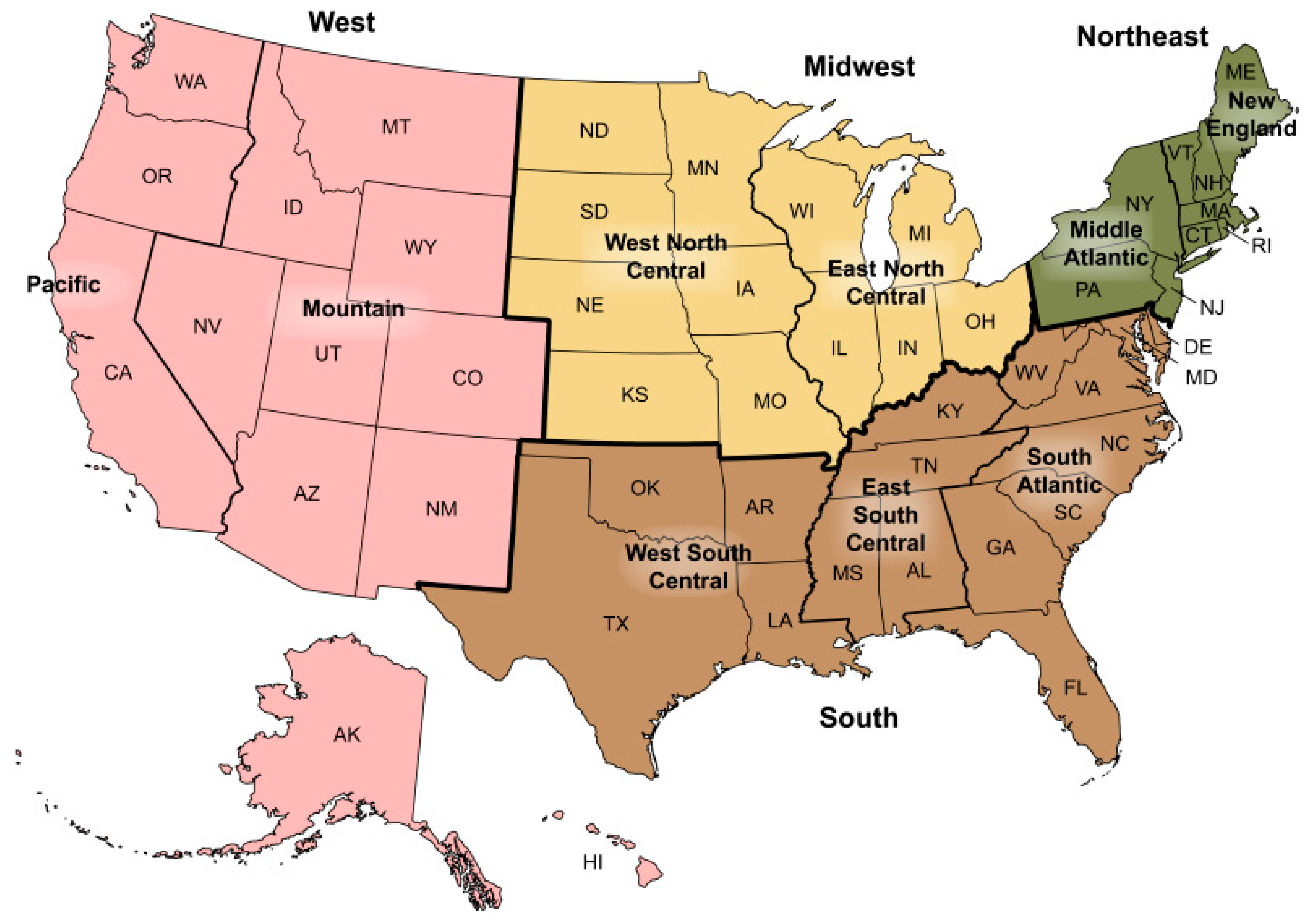
This study focuses on the Southern US, given the importance of agriculture in this region and its agroecological characteristics. According to the US Census Bureau, this region includes three divisions known as South Atlantic, East South-Central, and West South-Central, respectively, as shown in
Figure 1 below.
The South Atlantic division comprises eight states and one district: Delaware, District of Columbia, Florida, Georgia, Maryland, North Carolina, South Carolina, Virginia, and West Virginia. The East South-Central division includes four states: Alabama, Kentucky, Mississippi, and Tennessee. Finally, the West South-Central division comprises Arkansas, Louisiana, Oklahoma, and Texas. In terms of agronomic characteristics, the southern region varies significantly across states. Notably, there is a strong north-south variation in average temperatures. The northwest reaches of the region, which include the states of Kentucky and West Virginia, include cold regions in USDA plant hardiness zone 6 (−23.3 to −17.8 °C), while the southern reaches of the region, which include the state of Florida, include warm regions in plant hardiness zone 11 (4.4 to 10 °C). There is also an east-west gradient in precipitation that is evident in soil moisture regimes. The eastern reaches of the region are more wet with aquic and udic soil moisture regimes, while the western reaches of the region (i.e., Texas and Oklahoma) are more arid with udic ustic, typic ustic, and aridic ustic soil moisture regimes.
To increase productivity, it is fundamental to identify, understand, and analyze its main drivers. There are several factors that affect productivity. First, technological progress (TP)—which is defined as having access to better technologies to produce—has been identified as one of the main drivers of productivity growth worldwide [
21,
22,
23]. Second, technical efficiency (TE) that captures a farmer’s managerial ability. The overuse of inputs leads to inefficiency in the production process, suggesting that inefficient farmers can achieve their current levels of output while using fewer inputs. While having access to the best available technologies is a key component to increase productivity, knowing how to use them (i.e., being technically efficient) is a different question. Third, scale efficiency (SE) that captures whether a farm is using its optimal size of operations. Fourth, we account for state time-invariant specific characteristics. Finally, productivity is driven by changes in the production environment, i.e., climatic effects (CE) or conditions.
Therefore, the objectives of this study are threefold: (i) assess and analyze the impacts of climatic variability on agricultural production in the Southern US; (ii) calculate total factor productivity (TFP) across these states; (iii) identify the drivers of TFP growth. To achieve our objectives, we first use a stochastic production frontier (SPF) model to estimate the agricultural production function for the studied area. Then, we use the estimated parameters of the SPF to calculate, analyze, and decompose TFP into the aforementioned components: TP, TE, SE, CE, unobserved heterogeneity (UH), and statistical noise (SN) [
16,
24,
25].
The remainder of this paper is structured as follows:
Section 2 presents the methodological framework and data;
Section 3 presents the results; and
Section 4 concludes.
2. Materials and Methods
We use a SPF panel data approach to analyze the effects of climatic variability on agricultural production and productivity in 16 states in the southern region of the US. We assume that the Cobb–Douglas (CD) functional form can represent the underlying agricultural production technology of the SPF model and, thus, the estimated parameters are the partial elasticities of production. The CD functional form was used because it satisfies all the basic economic properties (i.e., non-negativity, monotonicity, and homogeneity) that are needed to derive the TFP framework used in this study, as opposed to a translog functional form [
26].
We estimate four empirical models with and without climatic variables using two alternative specifications, true fixed effects (TFE) and true random effects (TRE). The former specification is based on a maximum likelihood estimator (MLE), whereas the latter is based on a simulated MLE (SMLE). SMLE consists of maximizing the log likelihood based on a simulated estimate of the density function [
27]. The former model specification (TFE) assumes that state-specific, time-invariant unobserved heterogeneity (e.g., soil quality, unobserved environmental conditions) is correlated with the choice of inputs, whereas the latter model specification (TRE) assumes they are not (see Greene [
28]). Statistical tests are used to select the preferred model, and its associated estimates are used to calculate and decompose TFP growth by using the O’Donnell [
25] methods.
2.1. Panel Data Stochastic Production Frontiers
We start by presenting the methodological approach of the TFE and TRE SFP panel data models and explain the rationale behind each specification.
2.1.1. TFE Model
When conducting regression analyses with data that represent repeated observations of discrete entities such as geographical areas or states (as in our case), it is important to control for the entity-specific characteristics or effects that might affect the dependent variable. Unobservable factors may cause omitted variable bias, but if these factors are time-invariant and constant across entities, the TFE model is an appropriate approach [
27]. However, one potential limitation of TFE models is that they cannot assess the effect of variables that have little within-group variation [
28].
Formally, the TFE model can be expressed as follows:
where
denotes the natural logarithm (log) of agricultural production for the
i-th state in the
t-th time period;
is a (
1 ×
K) vector of inputs (expressed in logarithm), which includes capital, land, labor, intermediate inputs, and irrigation;
T is a time trend that captures technological progress;
is a random state-specific intercept parameter that captures time-invariant unobserved heterogeneity; and the other Greek letters are parameters to be estimated. The term
is a random error assumed to follow a normal distribution with mean zero and constant variance
, and
is a non-negative unobservable random term that captures the inefficiency of the
i-th state in period
. The inefficiency term
is assumed to follow a half-normal distribution. There are
NT observations (
N states during
T years).
Equation (1) can be modified to include climatic variables:
where the original parameters are as previously defined and
is a set of climatic variables expressed in levels that include annual mean temperature, annual mean precipitation, monthly standard deviation of mean temperature, and monthly standard deviation of precipitation. The specification of the climatic variables in Equation (2) follows the current strand of literature (e.g., see [
29] for an extensive literature review).
2.1.2. TRE Model
The TRE model enables controlling for time-invariant heterogeneity that is not correlated with input choices and climatic variables. This specification better handles variables such as temperature that slowly changes over time and can be expressed as follows:
This specification assumes that all the unmeasured heterogeneity (
) is uncorrelated with the included regressors. As before, this model is subsequently modified to incorporate climatic variables:
All variables are as defined before, and all models are estimated using the econometric package N-LOGIT 6.
2.1.3. Technical Efficiency
To calculate technical efficiency, we use the Jondrow et al. [
30] estimator to break down the composite error as follows:
where
, and
represents the signal-to-noise ratio that captures the weight of inefficiency in the total error term, or output variability. The terms
are the standard normal and conditional density functions, respectively.
2.1.4. Climate Adjusted Total Factor Productivity
We now turn to the calculation and decomposition of climate-adjusted TFP. The TFP index is the ratio of total output to all the inputs [
31]. Thus, the TFP index, which compares the TFP of state
at time
with that of state
in period
, can be expressed as follows:
Following O’Donnell [
25], Equation (6) can be rewritten as follows:
where the first right-hand term is an index that captures relative change in scale efficiency; the second represents technological progress; the third term is the change in climatic effects; the fourth component measures relative change in technical efficiency; and the last term captures statistical noise (SN). All Greek parameters are calculated as defined above, and
represents returns to scale.
2.2. Data
Our output–input dataset was obtained from the Economic Research Service (ERS) of the US Department of Agriculture (USDA). It is a panel dataset that covers 45 years and 16 states with a total of 720 observations. It contains one output, four conventional inputs, and four environmental variables. The output data are defined as gross production leaving the farm, and are an index constructed by combining physical quantities of crop production and livestock. The four inputs are capital, land, labor, and materials, and they are all indexes. Descriptive statistics are presented in
Table 1 below.
The capital index was constructed by obtaining data on rental prices and capital stock for each asset type, state, and the aggregate farm sector. The perpetual inventory method is used to develop stocks from data on investment for depreciable assets. Second, for land data, intertemporal price indexes of farmlands were created to obtain a constant quality land stock. The stock of land is then constructed implicitly as the ratio of the value of farmlands to the intertemporal price index. Here, aggregation is at the county level with the assumption that land in each county is homogeneous. To account for quality differences of land across states and regions, which prevented the direct comparison of observed prices, relative prices of land were calculated using hedonic regression results. Third, labor input data were calculated by using state-specific demographic data, such as age, sex, education, and employment class, which were obtained from the decennial census of population by the US Department of Commerce. Labor indexes were constructed by using demographically cross-classified hours and compensation data for each state and aggregate farm sector. Finally, intermediate input is covered as materials, which include goods used in production during the calendar year, such as pesticides, fertilizers, seeds, other purchased services, etc.
In addition, we use a set of climatic variables to capture the impacts of climate variability on production and productivity. State-level data for temperature and precipitation and the intra-standard deviation of temperature and precipitation are from the National Climatic Data Center (NCDC) of the National Oceanic and Atmospheric Administration (NOAA). Temperature and precipitation data are measured in Celsius and millimeters, respectively. According to Yang and Shumway [
32] and Lachaud et al. [
16], using aggregate climatic data makes empirical estimation possible in terms of identification and causality.
Irrigation data for states were obtained from the US Geological Survey, and they are measured in millions of gallons per day. The data were only available every five years. To obtain missing values for the remaining years, we used linear interpolation techniques. Specifically, the linear interpolation approach used in this study assumes that the estimates of missing values in a continuous range between two data points with known values can be computed using the following formula:
where
and
are the initial and later known values of two datapoints
and
, respectively, and
is the value of datapoint
which is to be found.
3. Results and Discussion
We estimate four different models including two alternative specifications (with and without climatic variables) and two distinctive econometric methods (TRE and TFE). These models are presented in
Table 2 and
Table 3 in the following order: Model 1, TRE
nc; Model 2, TFE
nc; Model 3, TRE
c; and Model 4, TFE
c, where the subscripts
nc and
c are used to differentiate models without and with climate variables, respectively. We use a CD functional form, as previously mentioned, to estimate all of them. We then compare the estimated models using statistical tests. Specifically, we compare TFE and TRE and then models with and without climatic variables (TFE
c and TRE
c). We then focus the discussion on the preferred model. Finally, we decompose TFP into its various components of efficiency and discuss their contribution to TFP growth.
3.1. Parameter Estimates
As shown in
Table 2 and
Table 3 below, the parameters for the variables that measure the conventional inputs are highly statistically significant across all estimated models. Regularity conditions from production economic theory, which require that partial output elasticities be nonnegative, are also satisfied across models. In addition, technological progress, which is captured by the parameter for the time trend, is significant at the 1% level, with a slight variation in Model 3. The estimated parameters for all the climatic variables are statistically significant across models, except for temperature in Model 4 (see
Table 3). Finally, the parameter
λ, which represents the signal-to-noise ratio, is highly significant across models, indicating that inefficiency plays a critical role in total output variability.
We then compare all the models using statistical tests to select the preferred one. First, we compare Model 1 vs. Model 2, and Model 3 vs. Model 4, using the Hausman test [
28]. Under the null hypothesis, the estimates of the TFE (Models 2 and 4) and TRE (Models 1 and 3) are both consistent, but only those of the TRE are efficient, whereas under the alternative hypothesis only the TFE estimates are consistent. Recall that the TRE models are built on the assumption of orthogonality of the random effect and the covariates [
27]. The results yield rejection of the null hypothesis with a large Hausman statistic, suggesting that TFE and TRE estimates are not similar. More precisely, the TRE estimates are inconsistent and affected by correlation bias between state-specific effects and the independent variables.
Specifically, under the null hypothesis, for Models 1 and 2 the Hausman test with a distribution has a statistic H = 2780.5 and a p-value = 0.000. Therefore, we reject the null hypothesis that the TRE model provides consistent estimates. Likewise, for Models 3 and 4 the Hausman test with a distribution has a statistic H = 3081.9 and a p-value = 0.000. Once again, we reject the null hypothesis that the TRE model provides consistent estimates.
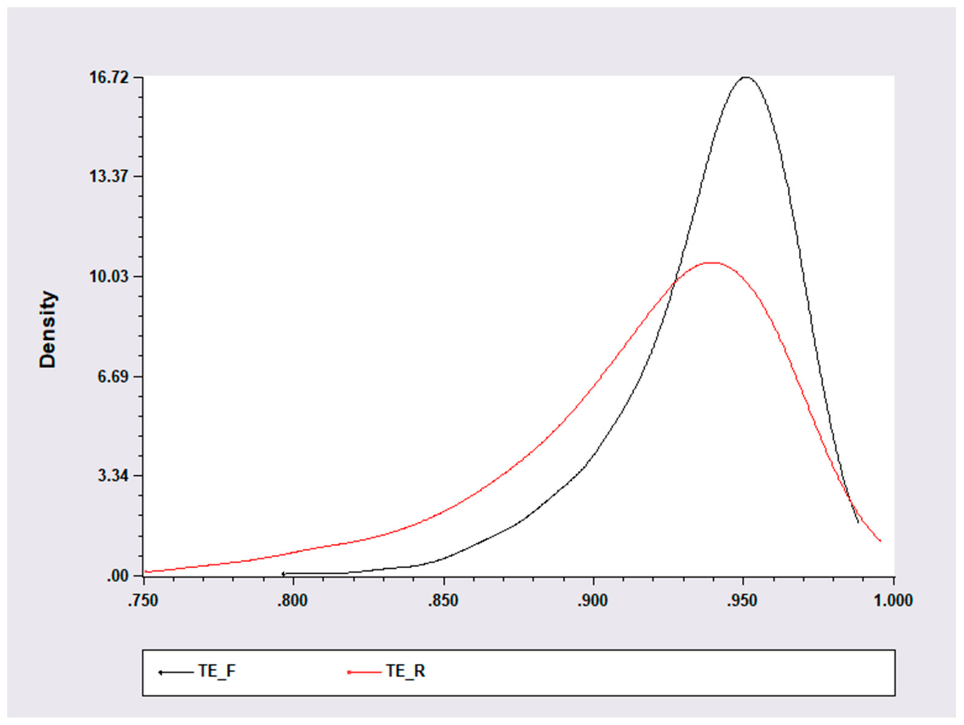
Furthermore, the difference between TFE and TRE can be better observed in
Figure 2 below. We compare TFE with climatic variables with its TRE counterpart, and the models report different efficiency estimates. For example, Model 3 displays efficiency means of 0.92 with standard deviations of 0.2, whereas Model 4 presents higher TE estimates with means of 0.96 that are less dispersed, with standard deviations of 0.01.
Now, we compare both TFE models, with and without climatic variables, using the Likelihood Ratio (LR) test [
28]. LR examines the goodness of fit of both models given the data (Models 2 and 4), based on the ratio of their likelihoods as reported in
Table 3. The results show that TFE with climatic variables outperforms TFE without climatic variables at the 1% level of significance. Thus, Model 4 is the preferred model, and we use the estimates obtained from this model to analyze and assess the impact of climatic variability on production and productivity.
As can be seen in
Table 3, the findings suggest that agricultural production in the southern US is most responsive to labor, and that production has been increasing at an annual growth rate of 1.3% across states due to technological progress. With regards to the impact of variables accounting for climatic fluctuations, annual precipitation has an overall, positive, and significant impact on agricultural production. However, the intra-annual standard deviation, a measure of variability, has a significant and negative impact. Both temperature and intra-annual deviation in temperature have a negative impact on production, but only the latter is statistically significant.
As expected, irrigation has a positive and significant impact on production. Specifically, our estimates suggest that if we increase irrigation by 100 million of gallons of water across all 16 states, agricultural production could increase, on average, by 3.7%. This result agrees with the negative impact on production related to variations in inter-annual precipitation presented earlier, since the availability of irrigation reduces the potential detrimental impact of droughts on crop yield, offers a more consistent availability of waters during the growing season, and lessens the effect of heat stress to both plans and animals during the summer month.
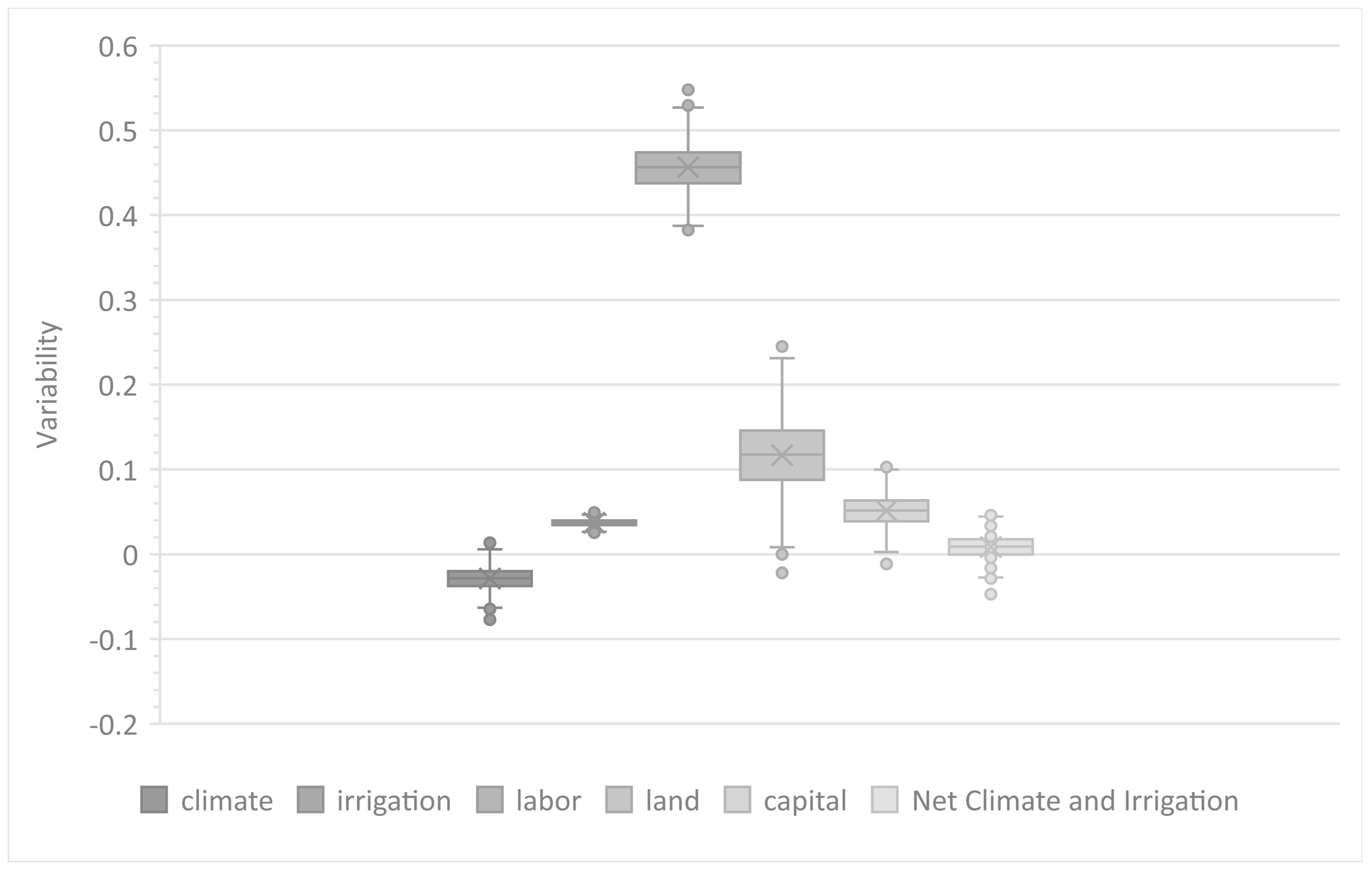
To better apprehend the magnitude of the impacts of climatic variability on agricultural production in the southern US, we can draw a comparison to other elements in the analysis (
Figure 3). To begin with, the total impact of climate effects must account for climatic conditions and variability and, therefore, must include the impact of temperature and precipitation, as well as the intra-annual variation in both. The comparison reveals that the single most important contributor to agricultural production is labor, and that the impact of labor is one or more orders of magnitude larger compared to that of the other inputs. However, the comparison also shows that the impact of climate is quite similar in magnitude (but opposite in sign) to the impact of irrigation. In practice, irrigation serves to smooth over climate variability, by providing water to crops during dry periods or at critical points in the growing cycle, and as a protection against frost. Thus, it can be expected that increased climatic variability may cancel out some or all of the marginal effects of irrigation on production. According to the analysis, the net effect of irrigation and climate effects on agricultural production was not statistically different from zero, implying that by 2004, most of the net gains of irrigation had been cancelled out by climatic variability effects.
3.2. TFP Decomposition
We now turn to the analysis of TFP, which we decompose into its multiple measures of efficiencies, using Equation (7).
Table 4 shows that over the period 1960–2004, average agricultural productivity increased by about 1.13 percent per year. All states have positive TFP growth. Agricultural productivity in West Virginia grew the fastest (1.42% per year), followed by Maryland, (1.26% per year), South Carolina (1.2% per year), and Louisiana (1.2% per year), whereas Oklahoma (0.99% per year), Arkansas (1.01% per year), and Kentucky (1.06% per year) display the slowest TFP growth. The last column in
Table 4 presents the specific constant for each state that captures state-specific time-invariant unobserved heterogeneity. The evidence shows that there is significant variability across states. Recall that this constant captures factors that we cannot observe or that we do not capture in the data, such as soil quality and other agronomic conditions that differ across states and have an impact on agricultural productivity.
Most states in the region have been producing below their frontier, i.e., they show the presence of inefficiency in production. In fact, among the 16 states in the sample, 10 of them have a negative TE growth. The evidence suggests that farms across these states are not operating at their optimal size, except for those in West Virginia. These results are not surprising, given that the technology they use exhibits decreasing returns to scale (See
Table 3).
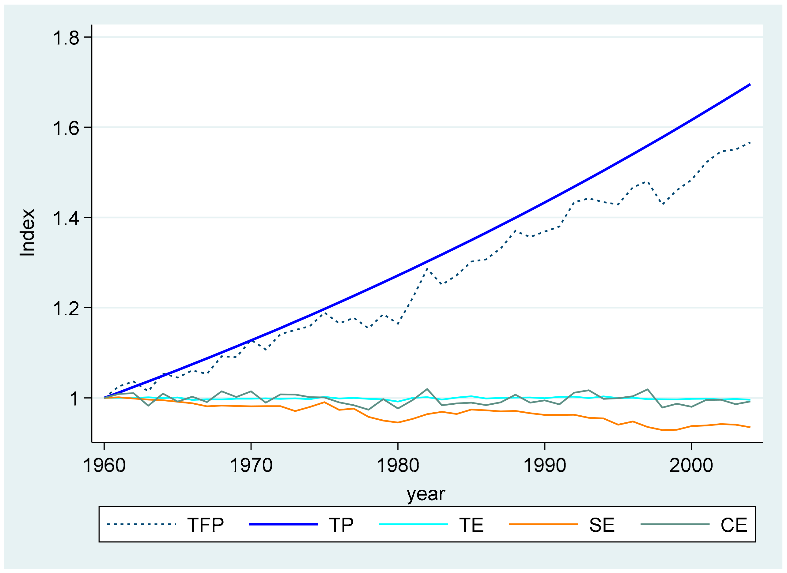
Figure 4 shows that technological progress has been the key driver of TFP, and it has increased, on average, at an annual growth rate of 1.26% (
Table 4). Technical efficiency components have remained quite flat, decreasing at an 0.01% annually, without much of an effect on productivity. Scale efficiency has been decreasing over time by 0.12% annually, and this result is not surprising given the nature of the technology’s decreasing returns to scale.
With respect to the impact of climate on agricultural productivity, the estimates for climatic effects show mixed effects, i.e., negative in some states and positive in others. Specifically, climatic variability has a negative effect on 10 states out of the 16, as can be seen in
Table 4, and its impacts are unevenly distributed. Before the 1980s, climatic variability captured by the CE index was above TE in an almost consistent manner over time, and then, on average, displayed a reverse trend, implying that the negative effect of productivity has increased over time in these states after the 1980s and, if this trend continues, the impact will be more severe in the coming years.
4. Conclusions
Agriculture or output variability is highly dependent on environmental factors, among other things, and the impact of climatic variability on agricultural production and productivity has been gaining attention in the past years. Despite the significance of this issue, up to now, very few studies have investigated its effects on agricultural productivity worldwide and, especially, on the southern region in the US. One of the main objectives of this study was to identify the main drivers of agricultural productivity in the southern US. This information can be useful for decision makers in the development of effective and sustainable agricultural policies [
33]. For example, we have demonstrated that the overall effect of climate change on agricultural productivity in the southern US has been negative, and that continued increases in climatic variability can cancel out the productivity gains from irrigation.
This study used input–output data from the USDA-ERS for 16 states over a 45-year period (1960–2004) to analyze the impact of climatic variability on agricultural production and productivity, accounting for unobserved heterogeneity across the states in the southern US. While it would have been preferable to use more recent data if they were available, the estimates of this study can be used to forecast TFP and all its components, as in Lachaud et al. [
21]. This exercise is beyond the scope and objectives of this study. The input–output data were augmented with average annual temperature and precipitation and intra-annual standard deviations of temperature and precipitation data from the NCDC, and by irrigation data from the US Geological Survey. The analysis relies on alternative SPF model specifications with and without climatic variables to estimate agricultural production functions for the region.
We found that agricultural production in the region is most responsive to labor and has been increasing over time at a rate of 1.3 percent annually. Technological progress was identified as the main driver of agricultural productivity (similar results are reported in [
34]). Several studies have reported that R&D spending is the main source of innovation and technological progress. Therefore, increasing federal and private funding for agricultural research is essential to improve and sustain agricultural productivity.
On the other hand, technical efficiency has been decreasing over time. It is important to recall that efficiency in production captures managerial skills and agricultural knowledge, and consequently, governs the ability of farmers to use the best management practices and available technologies. Thus, our results support the investment in extension programs that can help farmers in the southern US reach efficient levels of production. These types of policies would require increasing extension programs funding by federal, state, and local governments for researchers, universities, and other farm and agriculture organizations.
Our results also show that, on average, increasing precipitation has a positive and significant effect on production, and increasing temperature has a negative but non-significant impact. Intra-annual variations in precipitation and temperature, which could be considered as a measure of precipitation anomaly, have a negative impact on production. Further, the impact of climatic variability on agricultural productivity is mixed and unevenly distributed across the 16 states. In fact, it has a negative impact on 10 out of the 16 states in the region. Thus, to mitigate the negative impact of climate variability on agricultural production it is important for local and state governments to invest in climate adaptation strategies and mitigation programs, which can help farmers minimize the impact of climatic variability in the region. In fact, our results suggest that investing in irrigation could be an effective tool to mitigate climate effects in the studied areas.
While this study focuses only on the southern US, the impact of climatic variability on agricultural production and productivity is a global phenomenon with eventual severe consequences for food security in the US and worldwide. Farmers who are not landowners might be the most vulnerable and least able to cope with this problem. Investment in R&D to introduce new technologies, the main driver of TFP, should be oriented towards the development and use of climate-smart agriculture, the development of new varieties of plants that are adapted to variations in precipitation and temperature, and other farming strategies that are more resilient to climatic variability.


