A Critical Review of Current States of Practice in Direct Shear Testing of Unfilled Rock Fractures Focused on Multi-Stage and Boundary Conditions

Abstract

Direct shear (DS) is a common geotechnical laboratory test used to determine strength and deformation properties of rock discontinuities, such as normal and shear stiffness, peak and residual shear strength, and dilation. These are used as inputs for discontinuous geomechanical numerical models to simulate discontinuities discretely and shear strength is often expressed by Mohr–Coulomb, Patton, or Barton–Bandis constitutive models. This paper presents a critical review of the different boundary conditions and procedural techniques currently used in practice, summarizes previous contributions, addresses their impacts on interpreted results for rock engineering design, and introduces clarifying terminology for shear strength parameters. Based on the review, the authors advise that constant normal stress is best suited for discrete numerical-model-based rock engineering design in dry conditions, but constant normal stiffness should be considered where fluid permeability is of interest. Multi-stage testing should not be used to obtain peak shear strength values except for stage 1, because of accumulating asperity damage with successive shear stages. Nevertheless, if multi-stage testing must be employed due to limited budget or specimen availability, guidance is presented to improve shear strength results with limited displacement techniques.

1. Introduction

Direct shear testing is a common laboratory method used to measure geomechanical properties of rock discontinuities [1,2], including normal and shear stiffness (e.g., [3]), peak and residual shear strengths (e.g., [4]), and dilation angles (e.g., [5,6,7]). Measured shear strengths can be used to determine constitutive model parameters of linear and/or nonlinear failure envelopes. Linear methods commonly characterize discontinuities in terms of Mohr–Coulomb constitutive parameters: joint friction angle (φ) and joint shear strength y-intercept in shear stress versus normal stress space (apparent cohesion, c). Nonlinear approaches commonly use the Barton–Bandis constitutive model, which quantifies discontinuity shear strength in terms of joint roughness coefficient (JRC), joint compressive strength (JCS), and residual friction angle (φ_r) [4,8]. The accuracy of these calculated geomechanical properties partly depends on the selected laboratory test procedures used to measure the data in direct shear. Staged tests (e.g., single stage or multi-stage) and boundary conditions (e.g., constant normal load, constant normal stress, or constant normal stiffness) are the laboratory procedures that are the focus of this paper.

The current standard for laboratory direct shear testing (D5607-16) published by the American Society for Testing and Materials (ASTM) [9], along with the most recent suggested method published by the International Society for Rock Mechanics and Rock Engineering (ISRM) by Muralha et al. [2], state that at least three to five different normal loads are required to define a shear strength envelope [2,9]. To achieve this, there are two direct shear testing procedures that can be followed: (1) single-stage direct shear testing and (2) multi-stage direct shear testing. Under the multi-stage procedure, two techniques are described: (i) with repositioning of the specimen to zero displacement and (ii) without repositioning, between each stage. To address some of the limitations associated with multi-stage direct shear testing, an alternative procedure was proposed by Barla et al. [10] and Petro [11]. The proposed method limits the shear displacement within each stage of a multi-stage test to prevent extensive post-peak damage to the specimen and is referred to as limited displacement multi-stage direct shear testing (LDMDS) [11,12].

Over time, many researchers have questioned the validity of multi-stage testing as it has been observed to damage the surface of a specimen with successive shearing and impact the interpreted failure envelope strength parameters [11,12,13,14,15,16,17,18,19]. To evaluate the feasibility of multi-stage direct shear testing, test programs have been completed by various researchers to directly compare the results of single- and multi-stage tests and the interpreted Mohr–Coulomb parameters (e.g., [11,12,17,18,19]).

The ISRM suggested method by Muralha et al. [2] discusses constant normal load (CNL), constant normal stress (CNL*), and constant normal stiffness (CNS) boundary conditions for laboratory direct shear testing. The ASTM D5607-16 standard [9] only refers to the CNL condition, which was the first to be applied in laboratory research [20]. CNL and CNL* are unconstrained conditions that represent laboratory-scale analogues for fractures in near-ground surface environments where gravity-driven shear dominates [5,21]. In contrast, CNS is a constrained condition that represents deep underground environments where shear of rock fractures is driven by in situ and induced ground stresses near excavations (e.g., [20,22]).

It is important to note that the behaviour of a rock fracture can be generalized into two main categories: filled and unfilled fractures. The shear behaviour of an unfilled, clean, rock fracture is a function of the roughness and compressive strength of the fracture walls. On the other hand, filled fractures are mainly concerned with the physical and mineralogical properties of the infilling material [4]. The review presented herein is focused on unfilled, clean, rock fractures. Further, it is important to understand that the term discontinuity is often used to define several geological features, including, but not limited to, bedding planes, fractures, cleavage, veins, joints, and faults. In this paper, the term discontinuity is used interchangeably with the terms rock fracture and joint to identify a clean mechanical break in a rock mass with negligible tensile strength.

2. History of Direct Shear and Multi-Stage Testing

Direct shear testing has been a laboratory testing method used as early as 1776 by Coulomb, who, at that time, used it to determine the material properties of soils [23]. The practice of direct shear testing is still used today for the purposes of testing both soils and rock discontinuities.

The practice of multi-stage testing originally dates to 1950, where it was used in triaxial testing for the determination of soil strength properties. This original test was completed by De Beer, who stated “by increasing the axial load by steps and for each step determining the corresponding minimum lateral principal stress, a certain number of combinations of ultimate principal stress is obtained. The Mohr circles corresponding to these combinations can be drawn, and the envelope of these circles is determined” [24].

Taylor [25] confirmed the validity of this testing procedure for the use of determining peak shear strengths of a soil by completing a final stage following the testing program at the same pressure as stage 1 of the multi-stage testing program and comparing the results. Taylor observed that the final stage agreed with the first stage and deemed it was an acceptable procedure as long as the materials are not sensitive to a change in structure. These findings led to the belief that a multi-stage procedure was advantageous considering that the four-stage test gives as much information as four conventional single-stage tests and provides better information unless four identical samples can be collected [25].

Following the original multi-stage tests completed on soils, the first use of a multi-stage testing procedure on rocks was by Jaeger [26], who completed a series of multi-stage triaxial tests on natural joints and model joints (rock cylinders saw-cut at various angles to their axes) to gain information about the coefficient of friction and the process of sliding between rock surfaces. Shortly thereafter, Ripley and Lee [27] completed a series of multi-stage direct shear tests on both artificially smoothed and naturally rough surfaces of rock joints and separated bedding planes. Planar artificially smoothed surfaces were used to provide data on the basic friction properties of the materials and as a basis of comparison for assessing the effects of roughness on the sliding resistance of naturally rough surfaces [27]. This work by Ripley and Lee investigated the contribution that rough undulating surfaces have on the sliding resistance along planes of separation that extends beyond the contribution from simple friction between planar surfaces. This work is accredited with being the first published result that separates the effects of the geometry of the discontinuity from the coefficient of friction of the material [28]. During the study, the specimen surface in each subsequent stage was either washed or blown clean, and it was found that in all cases the initial stage produced values of resistance considerably higher than the subsequent stages. The difference in strength was attributed to the shearing of asperities during the initial stage and confirmed through visual observations [27].

The literature suggests that the practice of multi-stage testing for triaxial and direct shear testing of both rock and soil has been followed since some of the earliest research on direct shear testing (e.g., [25,27,29]). Although there was early evidence that its use impacts the strength results of later stages (e.g., [27]), the overall use of a multi-stage technique was viewed as an advantageous way to obtain additional data from a specimen using only one sample for testing as opposed to multiple samples [25,29,30]. A similar claim was made by Muralha [15], who stated “it is not practical to use a joint sample to perform a single shearing under a constant normal stress. Instead, several shearings under different normal stresses are performed on the same joint, enabling the assessment of its failure envelope”.

In the original suggested method for laboratory determination of direct shear strength published by the ISRM [1], the direct shear test was defined as a method of establishing values for peak and residual shear strengths of a test horizon. In the suggested method, the use of a multi-stage procedure was only detailed and suggested to establish additional residual strength values, with no mention of its use for determining additional peak shear strengths. After reaching a peak strength, the original ISRM reads “having established a residual strength the normal stress may be increased or reduced and shearing continued to obtain additional residual strength values” [1].

3. Current Practice for Laboratory Direct Shear Testing of Rock Fractures

Laboratory direct shear testing of rock specimens involves subjecting a specimen to a constant shear displacement rate under an applied normal load that is maintained under one of three boundary conditions: constant normal load (CNL), constant normal stress (CNL*), or constant normal stiffness (CNS). The appropriate selection of a boundary condition depends on the real-world application of the testing results and is discussed further in Section 4. It is worth noting that despite the boundary condition or staging technique used in a test, all direct shear testing machines incorporate the following components: a stiff testing frame, specimen holder, normal and shear loading devices, load and displacement monitoring instrumentation, pressure-maintaining devices, and data acquisition equipment. They can also be servo-controlled, meaning that a user-defined computer program controls the load and displacements of the direct shear machine and records data throughout the test. The programming of the servo-controlled component may vary depending on the testing regime. The setup of a typical direct shear testing apparatus is illustrated in Figure 1.

In general, all three boundary conditions begin with the application of a target normal load or stress to the test specimen, followed by application of a shear force at a constant shear displacement rate until the yield, peak, and then residual shear strengths are achieved. In some cases, two different peak shear strengths may occur. Examples of these shear strength parameters measured from direct shear test data are shown in Figure 2.

Yield shear strength is the onset of nonlinear behaviour following elastic loading and is commonly defined as the point of maximum curvature [31]. The first peak shear strength typically occurs shortly after yield and is followed by the first decrease in shear stress. This is commonly referred to as the peak shear strength and is typically observed in all three boundary conditions (CNL, CNL*, and CNS). Upon additional shear displacement after the first peak shear strength, residual shear strength is typically observed under CNL and CNL* boundary conditions. However, under CNS boundary conditions, a second peak shear stress may occur prior to reaching residual. Due to a variety of terminologies in the literature for first and second peak shear strengths, it is difficult to distinguish between these important parameters. To overcome variations in the definitions of peak shear strength under different boundary conditions, the authors propose the following blanket terminology that can be used for direct shear tests under any boundary condition (CNL, CNL*, or CNS).

Unconstrained peak shear strength (τ_p-u) refers to the maximum attainable shear stress followed by the first decrease in shear stress immediately following yield. Under CNL and CNL* conditions, there is no constraint on the specimen’s ability to dilate. However, under CNS boundary conditions (that allow dilation to be constrained), the applied normal stress at this point is either equal to or very close to the initial normal stress level and is regarded as unconstrained. It is worth noting that yield and unconstrained peak shear strengths may be equivalent in some cases.

Constrained peak shear strength (τ_p-c) applies to the maximum attainable shear stress that may occur with additional shear displacement following τ_p-u. This (second) peak shear strength is more commonly observed under CNS boundary conditions where KNM > 0. The introduction of a positive KNM will lead to an increase in the applied normal stress as a response to positive normal displacement to constrain the experienced dilation during shear testing.

The sustained shear stress in the post-peak region is referred to as the residual or ultimate shear strength. To define a shear strength envelope, ISRM and ASTM require three to five shear strengths measured at different normal loads. To achieve this, three methods have been developed: single-stage, multi-stage, and limited displacement multi-stage direct shear testing. Currently, only the first two methods are described in detail by the ISRM Suggested Methods [1,2] and ASTM Standard [9]. Limited displacement multi-stage direct shear testing is a more recent development and is described by several authors [10,11,12]. The details of each staging methodology are further discussed in Section 5.

Figure 2. Example of shear stress versus shear displacement direct shear test data with common linear shear stiffness measurements and shear strength parameters for (a) rough, clean limestone joint under constant normal stress (CNL*) boundary condition (modified after [6,32]); (b) rough, clean granitic crystalline joint under constant normal stiffness (CNS) boundary condition (modified after [7]).

Figure 2. Example of shear stress versus shear displacement direct shear test data with common linear shear stiffness measurements and shear strength parameters for (a) rough, clean limestone joint under constant normal stress (CNL*) boundary condition (modified after [6,32]); (b) rough, clean granitic crystalline joint under constant normal stiffness (CNS) boundary condition (modified after [7]).

4. Direct Shear Test Boundary Conditions

In laboratory direct shear testing, it is necessary to define the boundary condition under which a sample will be tested. The purpose of varying boundary conditions is to simulate real world stress conditions. In general, this can be simplified into two external conditions: (i) the normal stress remains relatively constant during shearing (achieved with CNL or CNL* boundary conditions); and (ii) the normal stress varies during shearing (achieved with a CNS boundary condition). Each boundary condition is representative of different scenarios that may be encountered in rock engineering designs (e.g., [20,33]).

The use of CNL or CNL* boundary conditions represents fracture behaviour in slopes and other near surface gravity driven environments in which the applied normal load or stress remains constant (Figure 3a). Alternatively, a CNS boundary condition is representative of rock fractures near underground excavations such as tunnels, mines, and nuclear waste repositories in which sliding blocks are constrained between parallel dilatant joints where little to no normal displacement occurs, or a controlled stiffness response occurs [20], as illustrated in Figure 3b. In these respective conditions, under CNL/CNL*, the fracture is free to dilate during shearing with no feedback between dilation and normal stress, whereas under CNS conditions, dilation is constrained by feedback between dilation and normal stress to maintain a constant machine stiffness. The details of dilation behaviour in each of these boundary conditions are described and illustrated in the following sections.

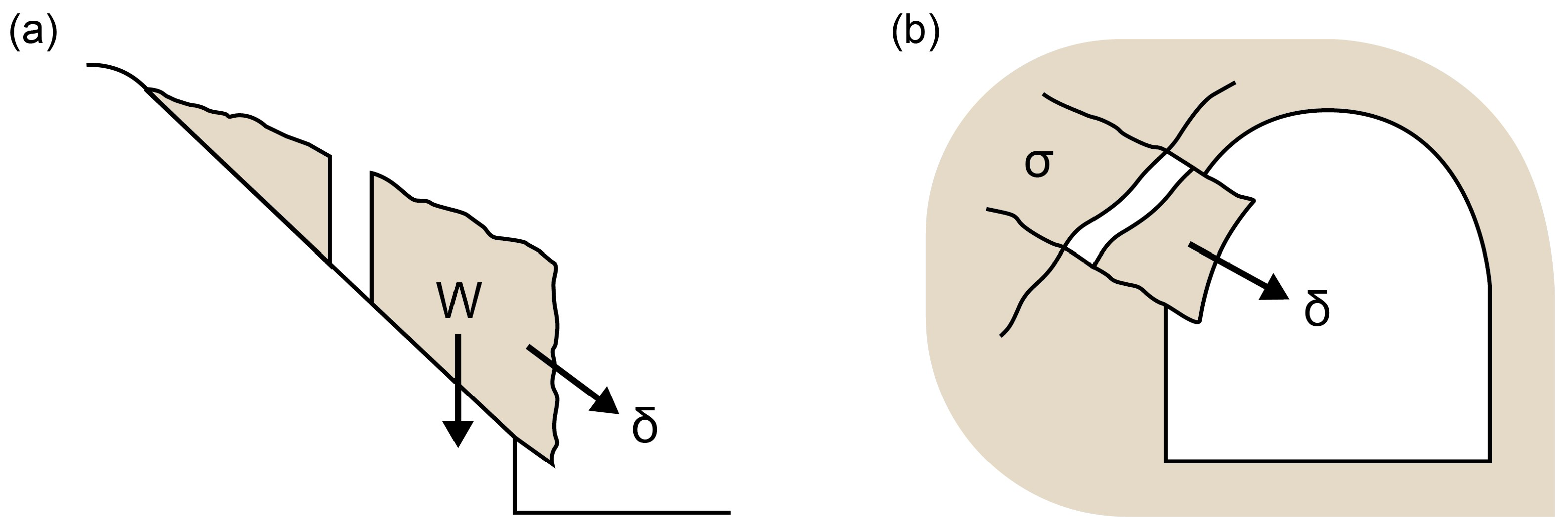
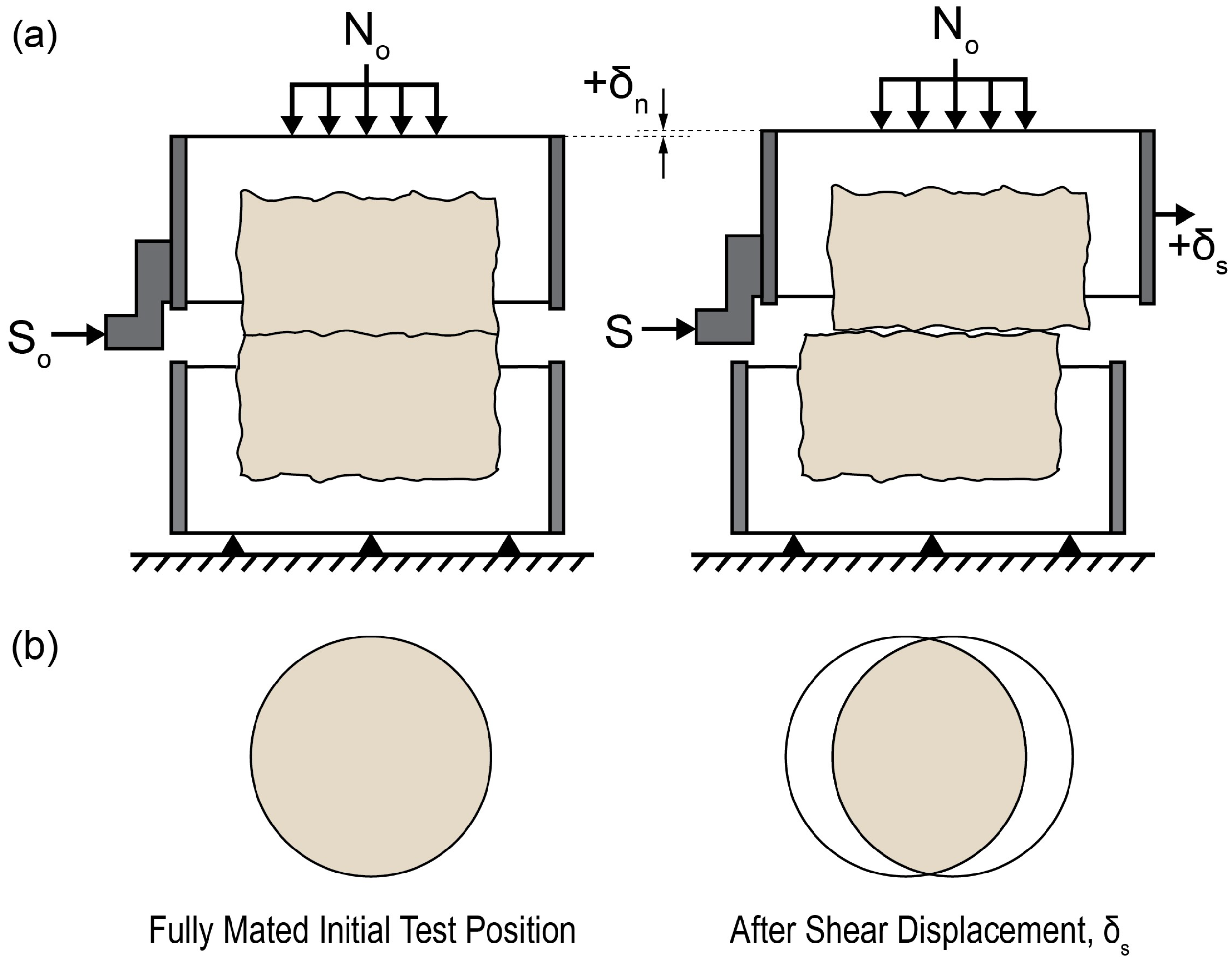
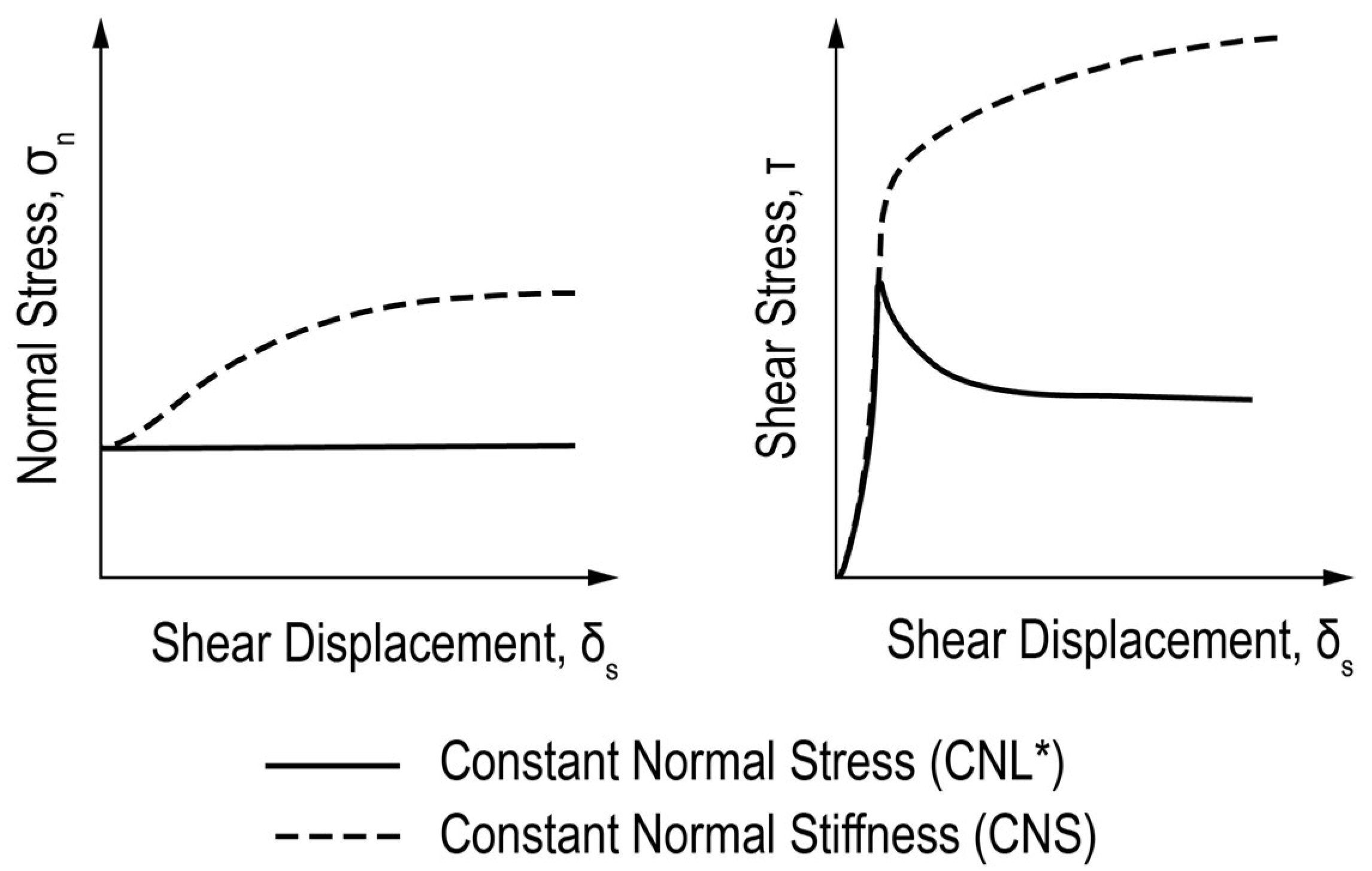
4.1. Constant Normal Load (CNL) and Constant Normal Stress (CNL*)

Constant normal load (CNL) is the conventional and first-used boundary condition for laboratory direct shear testing [20]. CNL testing is achieved by applying a normal load to the specimen using either weights or hydraulic pressure (depending on the mechanics of the machine), which remains constant for the duration of a direct shear test. More recently, the development of servo-controlled laboratory direct shear machines has made it possible to complete direct shear tests under CNL* boundary conditions. A servo-controlled machine is an automated device that uses a negative feedback loop from the system to adjust internal mechanisms to minimize the error between the machine input and the machine output [34]. For CNL and CNL* testing, a measurement of normal stress lower than the input would prompt the machine to increase the normal load until the desired normal stress is achieved during shear displacement. Based on an input geometry representing the cross-sectional target shear area of the specimen, the servo-controlled direct shear machine can calculate and update the contact surface area at any shear displacement. Knowing the change in surface area and the rate at which shear displacement occurs, the servo-controlled machine can continuously calculate and update the required applied normal load for the duration of a shear test. This continuous feedback allows for the applied normal load to vary accordingly and maintain a constant normal stress. An example of changing contact surface area of a specimen during a CNL or CNL* direct shear test is illustrated in Figure 4.

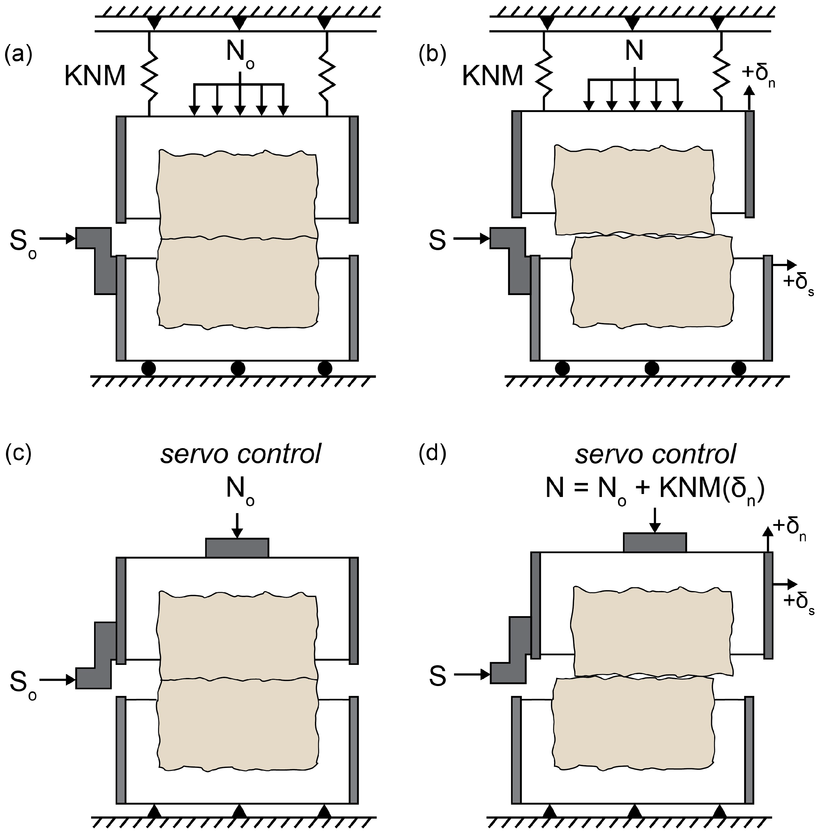
4.2. Constant Normal Stiffness (CNS)

Although the use of CNL and CNL* boundary conditions are representative of near-surface projects where a fracture is free to dilate, it is considered unrepresentative for projects at depth where the dilation of a fracture is constrained by the surrounding rock mass. This was confirmed in a study conducted by [35], who concluded that a CNS boundary condition should be applied to jointed rock masses in which dilation is constrained as there is a strengthening effect due to the normal stiffness of the rock mass. Johnston et al. [22] further studied the boundary between cast-in-place concrete piles and a sandstone rock mass and concluded that a CNS boundary condition can be applied to better represent the shear behaviour of rough rock joints when dilation is constrained. A CNS boundary condition involves restricting a fracture’s ability to dilate, resulting in an increase in the applied normal stress, which in turn increases the measured shear strength of a fracture [35,36,37]. The change in the applied normal load ($∆F_n$) to the test specimen depends on the change in normal displacement ($∆{\delta }_n$) of the specimen and normal stiffness of the machine ($KNM$), as mathematically described in Equation (1) [35], where $KNM$ is the machine normal stiffness, $N$ is the applied normal stress, and $N_o$ is the initial applied normal stress. Readers are directed to [7] for additional detail.

$$N=N_o+∆F_n=N_o+KNM\left(∆{\delta }_n\right)$$

(1)

The CNS boundary condition can be implemented using two types of machines: (i) a CNL machine outfitted with springs of known stiffness or (ii) a servo-controlled direct shear machine [38]. For a spring-outfitted CNL machine, the bottom half of the specimen box is constrained to movements in the horizontal direction and the top half of the specimen box is rigidly constrained so that it can only move in the vertical direction. Furthermore, to simulate CNS conditions, the constrained top half of the box can only move against a spring of known stiffness. The steel shaft transmits the normal force through a load cell and a screw jack to a suspended spring system mounted at the top of the frame [22] (Figure 5a,b). For a servo-controlled machine, a negative feedback loop is used to satisfy a user-defined constant machine normal stiffness (KNM) (Figure 5c,d). This is achieved as the normal actuator holds the machine stiffness constant and the feedback loop increases or decreases the applied normal load based on an empirical relationship used to represent the normal stiffness of a rock mass. As a joint begins to dilate, negative feedback will be prompted, and the machine will correct for the change in normal displacement by increasing the applied normal load. On the contrary, in the case where a joint begins to contract, a negative feedback loop will prompt the machine to decrease the load to maintain a constant normal stiffness. At points where there is no dilation (and no increase or decrease of the normal load due to dilation or contraction), the machine will hold the normal load constant rather than the normal stress constant [7].

For underground tunnelling applications, machine normal stiffness ($KNM$) can be calculated based on the elastic properties of a rock block (Young’s modulus, $E$, and Poisson’s ratio, $\nu$), joint spacing in the rock mass, $L$, and the test fracture surface area, $A$, with Equation (2) by Packulak et al. [7]. For additional methods to calculate machine normal stiffness for different applications, readers are encouraged to read Johnston et al. [22] and Skinas et al. [39].

$$KNM=\frac{E}{2L\left(1-{\nu }^2\right)}A$$

(2)

5. Single- and Multi-Stage Direct Shear Testing

The conventional approach for direct shear testing is to follow a single-stage testing procedure, which involves testing a minimum of three to five different specimens that are similar in nature and come from the same discontinuity or sampling horizon. Each specimen is tested at a different normal stress and the results are used to define a shear strength envelope of the discontinuity. A single-stage test is complete once the residual shear stress for the tested specimen is defined [2,9]. The idealized results for four typical single-stage direct shear tests at different normal loads under CNL/CNL* boundary conditions and their corresponding failure envelopes are illustrated in Figure 6a.

5.1. Conventional Multi-Stage Direct Shear Testing

In practice, it is often difficult and/or expensive to obtain several specimens from the same discontinuity or discontinuity set that are similar in nature for the purpose of completing multiple single-stage tests. As a result, it has become common practice to repeatedly test the same specimen under several increasing normal stresses to define a failure envelope. Similar to the single-stage procedure, a minimum of three to five normal stresses are required to define the failure envelope. In contrast to a single-stage test, once the residual shear stress for a specimen is achieved, this indicates the completion of stage 1. Following stage 1, an additional two to four stages are required to be completed on the same specimen. When using a multi-stage testing procedure, there are two methods that can be followed for the subsequent stages: (i) multi-stage without repositioning (Figure 6b); and (ii) multi-stage with repositioning (Figure 6d). The practice of repositioning involves returning the specimen to zero shear displacement between each stage prior to increasing the normal load. Alternatively, the specimen can begin subsequent stages at the final position of the previous shear stage [2,9]. In terms of the applied normal load for each stage, it is recommended by ASTM D5607-16 [9] that each consecutive stage should be performed with a higher normal load, starting at the lowest required normal load, to reduce the potential for the effects of specimen degradation and wear. It is worth emphasizing that the current ASTM standard details that prior to increasing the normal load for each subsequent stage, residual strength is required to be established.

At this point it is worth clarifying a key difference between the 1974 and 2014 ISRM publications. As opposed to the original 1974 ISRM Suggested Method, the updated 2014 ISRM Suggested Method has retracted its statement of using multi-stage testing to obtain additional residual strength values and now states “Using the data records and the shear stress versus shear displacement graphs, evaluate the peak and ultimate or residual shear stress for each sample of the same rock joint or test horizon in the case of single stage tests, or for all stages of multi-stage tests of the same rock sample” [2]. The same statement is made for obtaining peak and/or residual dilation angles. Although the use of multi-stage results is considered for the determination of peak and residual parameters, the limitations of multi-stage testing do not go unnoticed. Within the same ISRM Suggested Method, a cautionary statement is made that reads “In the case of multi-stage tests, the apparent cohesion can be exaggerated due to accumulation of damage with successive shearing of the same joint specimen” [2].

5.2. Limited Displacement Multi-Stage Direct Shear Testing

The multi-stage direct shear testing method described by the ISRM and ASTM (and here in Section 5.1) results in the accumulation of damage to the discontinuity surface as the specimen is sheared to its residual shear strength for each shear stage. To prevent extensive asperity damage and limit the shear displacement during each stage, Barla et al. [10] developed an alternative procedure, which was later termed by Petro [11] as the limited displacement multi-stage direct shear (LDMDS) test. This technique, which has been conducted only under CNL or CNL* boundary conditions, limits the damage by pausing the shear displacement once the unconstrained peak shear strength is achieved and is designed to not slip past the first critical asperity. Once paused, the normal load/stress is increased to the next desired load/stress, and shear displacement is resumed. Once the unconstrained peak shear strengths are measured for each normal load/stress magnitude, residual shear strength can then be defined [10,11,12]. An example of a shear stress versus shear displacement curve of an LDMDS test is shown in Figure 6c.

6. Shear Behaviour of Clean Rock Joints

The shear strength of a discontinuity in rock has been observed to be controlled by several components, including joint size, joint roughness, joint compressive strength, asperity height, asperity angle, joint weathering, joint infill material(s), joint loading history, and stress conditions (among others, [4,5,40,41]). As there are several components that influence the shear behaviour of a discontinuity, it is important to understand the fundamentals of each one and how it impacts shear behaviour. Many analytical and experimental studies have been completed to investigate empirical relationships using single-stage laboratory testing under CNL/CNL* boundary conditions (e.g., [42,43,44,45]) and CNS boundary conditions (e.g., [38,46,47]). Thirukumaran and Indraratna [48] present further discussion on the shear strength constitutive models specifically for rock joints subjected to CNS boundary conditions. With the increased use of computational tools over the past few decades, research has started to focus on how numerical codes predict how fractures will behave when sheared (e.g., [49,50,51]).

As shear strength is dependent on normal stress, many researchers have developed empirical relationships that rely on various input parameters (among others, [4,8,21,41,44,52,53,54,55]. Many of these constitutive models have been created using empirical relationships based on field observations and laboratory results, while some have been developed based on theory. Regardless, it is important to understand that each constitutive model has been developed under certain boundary conditions and assumptions that may not hold true to every scenario. Of these, there are three main shear strength criteria for rock discontinuities that are commonly referenced and expanded on in the literature: Mohr–Coulomb’s linear shear strength criterion [52], Patton’s bilinear failure envelope [53], and Barton–Bandis’ nonlinear shear strength criterion [8].

This section provides an overview of these three common shear strength criteria and the shear failure mechanism of rock joints in a simplified manner.

6.1. Common Shear Strength Criteria for Rock Fractures

6.1.1. Mohr–Coulomb Linear Shear Strength Criterion

The linear Mohr–Coulomb shear strength criterion is the oldest constitutive model created to quantify the shear strength of soils and is described by Equation (3) [52]. The Mohr–Coulomb model has been adopted into the rock mechanics field to describe both the shear strength of intact rock and rock discontinuities. As it has been adopted from soil mechanics, the Mohr–Coulomb criterion is subject to several limitations as it does not take into consideration the surface profile and roughness, the geological material, asperity order, weathering, or stress history. Despite its limitations, this shear strength criterion remains perhaps the most widely used today.

$$\tau ={\sigma }_n\ast \tan \mathsf{\varphi }+\mathrm{c}$$

(3)

where $\tau$ is maximum shear strength, ${\sigma }_n$ is the applied normal stress, ϕ is the friction angle, and c represents cohesion [52]. The units of these parameters in rock mechanics are typically expressed in degrees (°) for friction angle, and megapascals (MPa) for all of shear stress, normal stress, and cohesion.

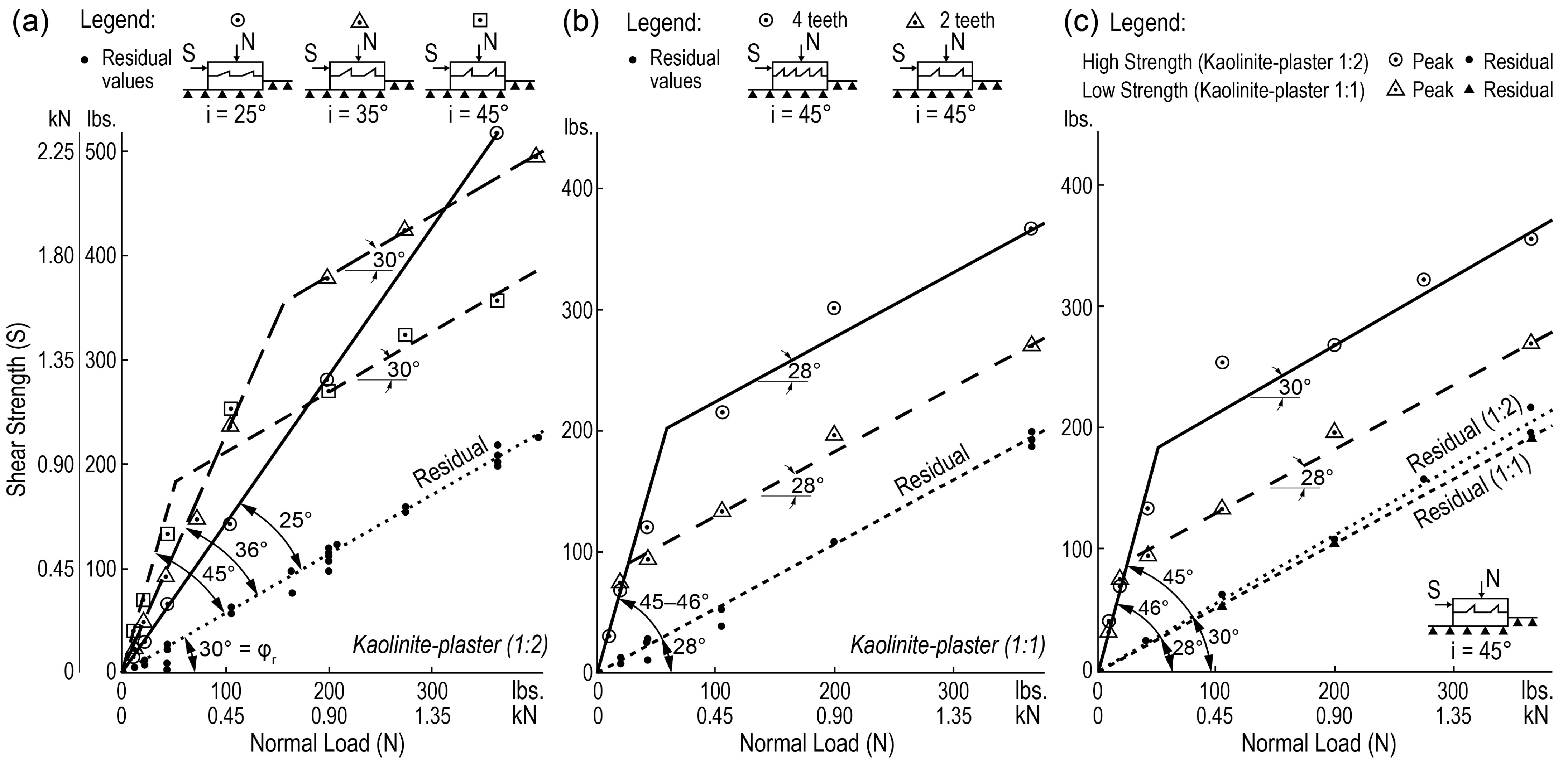
6.1.2. Patton Bilinear Shear Strength Criterion

The bilinear Patton constitutive model was one of the earliest models created to describe the modes of failure for laboratory direct shear testing of rough rock joints [56]. Patton completed a series of laboratory direct shear tests on artificial sawtooth joints to evaluate the different modes of failure. From his results, Patton verified an observation that was originally noted by Newland and Allely [57], who suggested that the differences between the angle of sliding friction, ϕ_μ, and the angle of internal friction, ϕ_f, can be explained through the mode of failure, which itself is a function of ϕ_μ. Patton observed that the failure envelopes are better approximated by two straight lines as opposed to one, whereby the inflection point is related to a change in the mode of failure from sliding to shearing, as shown in Figure 7 [53]. Patton completed a series of direct shear tests to develop failure envelopes and changed one variable each time. Figure 7 illustrates Patton’s findings when varying (a) the inclination of the artificial teeth, (b) the number of artificial teeth, and (c) the internal strength of the artificial teeth [53]. From his research, Patton observed that the data points plotting along the steeply sloping (primary) portion of the envelope are approximately equal to ϕ_μ + i (where i is the inclination from horizontal of saw tooth asperities), whereas the data plotting along the secondary portion of the envelope are approximately equal to ϕ_r [53]. As a result, Patton concluded that ϕ does not vary throughout a wide range of normal loads (although ϕ + i does) and that changes in the mode of failure are related to the physical properties of irregularities along the failure surface [56]. He further suggested that the vertical distance between a peak failure envelope and residual failure envelope is the strength contributed from the irregularities on the surface.

Patton [56] proposed two equations to express the shear strength of rock joints with inclined teeth for a single direction of shearing. Equation (4) represents the steeper (primary) portion of the bilinear failure envelope at lower normal stresses (where sliding over asperities dominates the shear mechanism) and Equation (5) represents the secondary portion at higher normal stresses (where shearing through asperities dominates the shear mechanism) of the envelope:

$$\tau ={\sigma }_n\ast \mathrm{t}\mathrm{a}\mathrm{n} ({\mathsf{\varphi }}_b+i)$$

(4)

$$\tau =c+{\sigma }_n\ast \mathrm{t}\mathrm{a}\mathrm{n} \left({\mathsf{\varphi }}_r\right)$$

(5)

where $\tau$ is the total shear strength, ${\sigma }_n$ is the applied normal stress, ${\mathsf{\varphi }}_b$ is the basic friction angle, i is the angle of inclination of the teeth from the horizontal, $c$ is the cohesion intercept (mobilized when teeth are sheared off at their base), and ${\mathsf{\varphi }}_r$ is the angle of residual shearing resistance [53].

The bilinear Patton [53] constitutive model is similar to the Mohr–Coulomb [52] model in that both can be described in terms of cohesion (c) and friction angle (ϕ). As opposed to developing a failure envelope using Equations (4) and (5), a single straight line would be used to define the shear failure envelope of the rock fracture, giving it a nonzero positive shear strength at an applied normal stress of 0, commonly referred to as apparent cohesion. Patton [53] notes the limitations to this method, as a single line would suggest only one mode of failure and assumes a nonzero cohesive strength at zero to low normal stresses which may be incorrect. True cohesive strength is present when cemented surfaces are sheared and represents the strength of the cementing material [58]. Rock joints that are clean (with no infilling) will have zero cohesive strength at zero to low confinement and their strength will be defined by the friction angle. Figure 8 illustrates the relationships between shear and normal stresses on a sliding surface for five different geological scenarios at a range of normal stress conditions [58].

In contrast to the idea of a joint having zero cohesive strength for an applied normal stress of 0 MPa, the observed cohesion is the result of the interlocking surfaces of nonplanar joints. Goodman et al. [3] state that through the cohesion due to interlocking asperities, the joint strength is related to the wall rock strength.

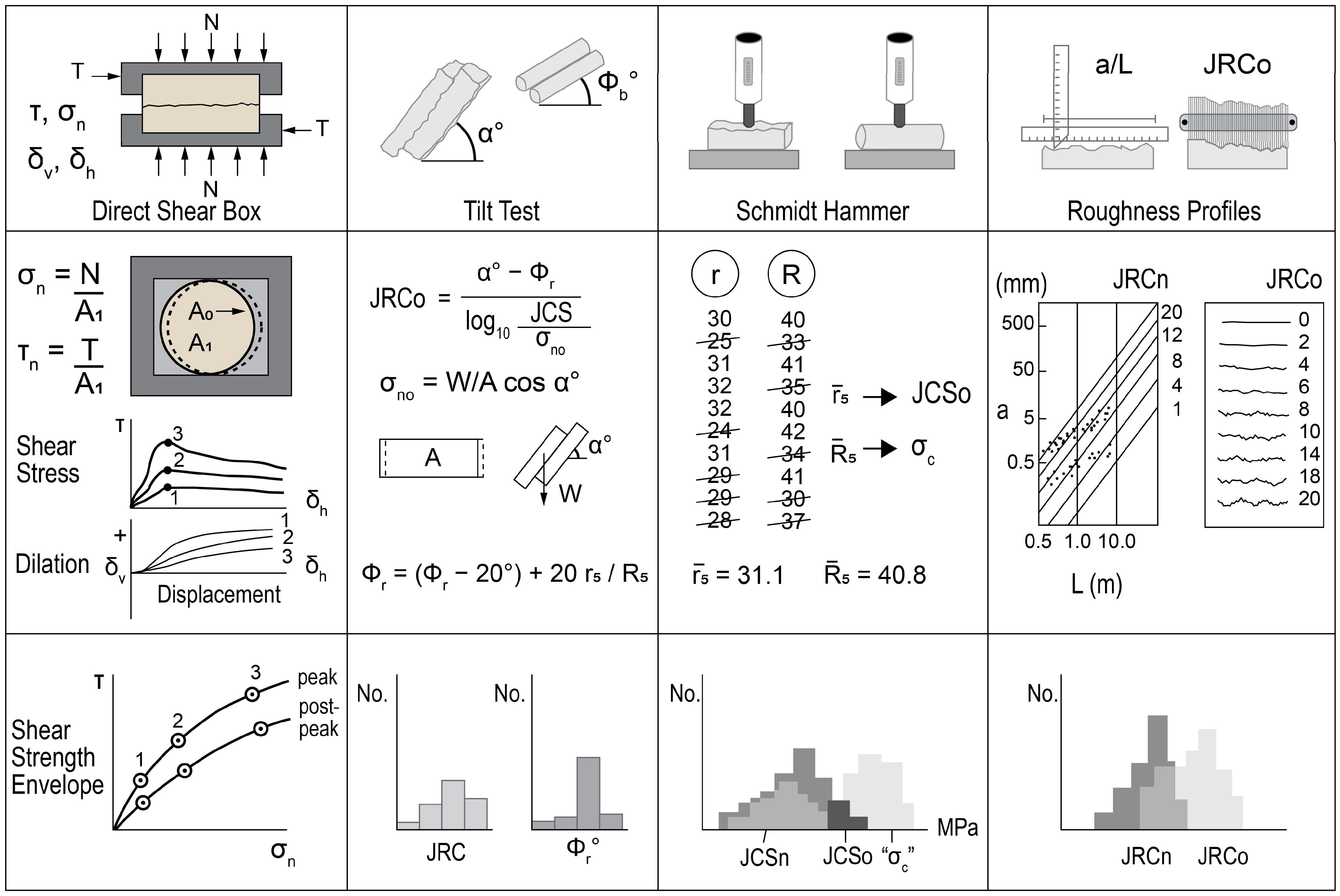
6.1.3. Barton–Bandis Nonlinear Shear Strength Criterion

This nonlinear constitutive model is an empirical relationship for shear strength of rock fractures (i.e., joints) that was originally developed to be used in three different ways: (i) curve fitting to experimental peak shear strength data; (ii) extrapolation of experimental peak shear strength data; and (iii) prediction of peak shear strength data [4]. Over time, the equation has been revisited by the author and the up-to-date equation is expressed by Equation (6) [8]. Equation (6) contains three main parameters that vary shear strength ($\tau$, MPa) with respect to the applied effective normal stress (${\sigma }_n$, MPa), depending on the joint character: joint roughness coefficient ($JRC$, unitless), joint wall compressive strength ($JCS$, MPa), and the residual friction angle (${\mathsf{\varphi }}_r$, °) [4,59]. Figure 9 contains three peak shear strength envelopes that were calculated using Equation (6) to illustrate the nature of the empirical law, and the effects that both $JRC$ and $JCS$ have on peak shear strength [4].

$$\tau ={\sigma }_n\ast \mathrm{t}\mathrm{a}\mathrm{n} (JRC\ast \log \frac{JCS}{{\sigma }_n}+{\mathsf{\varphi }}_r)$$

(6)

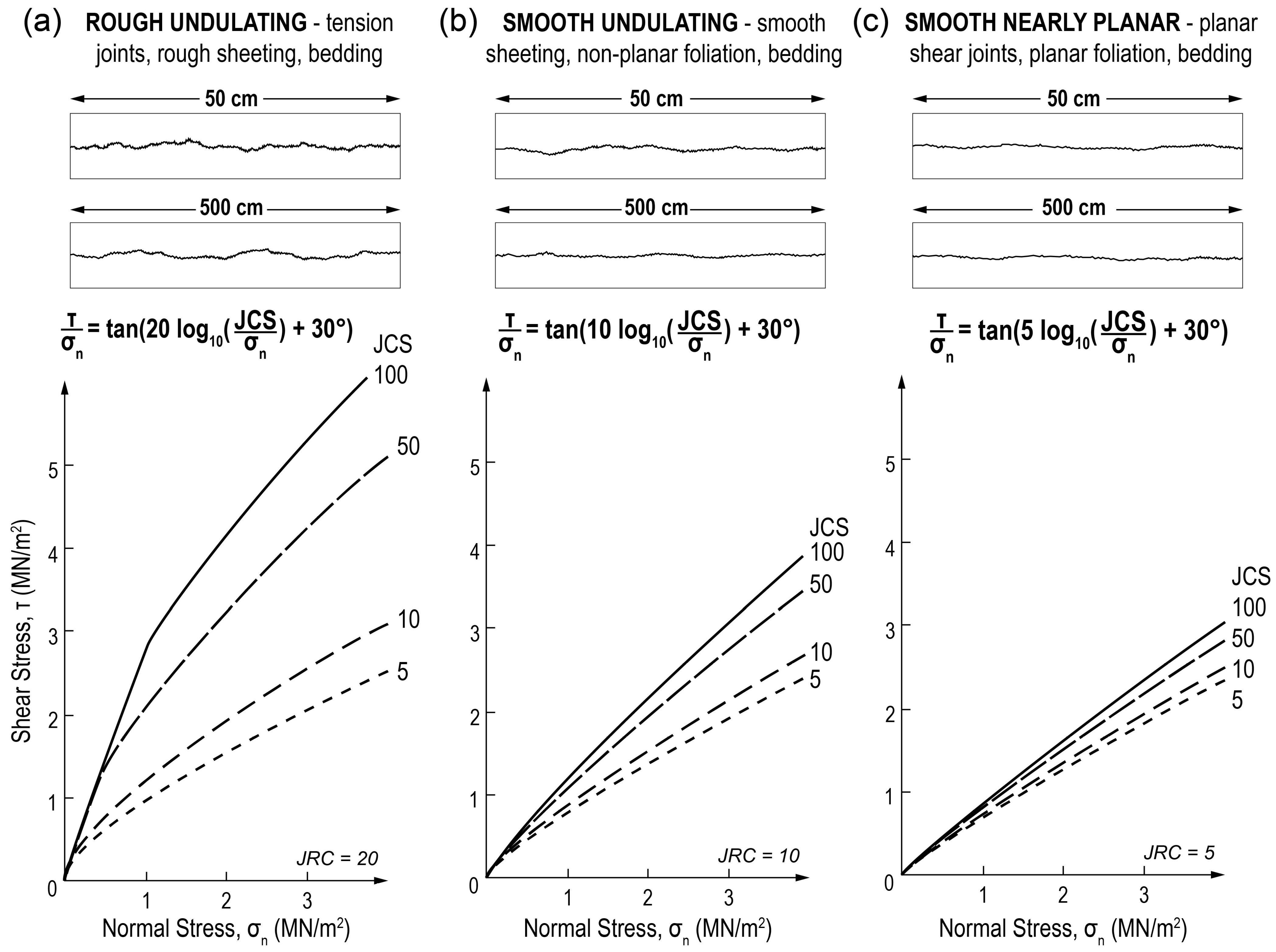
Joint Roughness Coefficient

The joint roughness coefficient was originally introduced in Barton’s [5] shear strength criterion as a method to define a joint’s surface profile in terms of roughness and quantify it for use in his empirical equation. To define $JRC$, Equation (6) can be rearranged to give Equation (7).

$$JRC=\frac{{\tan }^{-1}\left(\tau /{\sigma }_n\right)-{\mathsf{\varphi }}_r}{\log \left(\frac{JCS}{{\sigma }_n}\right)}$$

(7)

In the event that shear stress data are unavailable, Barton and Choubey [4] presented an alternative method to crudely estimate the JRC of a joint. This method involves visually comparing the roughness profile for the joint in question to a series of typical roughness profiles. The 10 typical roughness profiles were based on 136 tested joint specimens and are illustrated here in Figure 10. Although this method is still commonly used today, it was originally stated that the most satisfactory method to obtain JRC is by back-calculation, based on a tilt and/or push/pull test. In this instance, the angle at which sliding occurs represents $({\tan }^{-1}\left(\tau /{\sigma }_n\right))$ in Equation (7) and the shear stress and normal stress are generated by the weight of the top half of the specimen [4]. It is acknowledged and emphasized by Barton and Oslo [60] that the “ten JRC profiles” were only developed to illustrate the range of surfaces tested and that using them to represent a surface’s roughness is far too subjective a method.

Joint Compressive Strength

Similar to JRC, joint compressive strength (JCS) was introduced in Barton’s [5] shear strength criterion as a method to define the compressive strength of a joint. The introduction of JCS allows for shear strength estimations while considering the effects of joint alteration (weathering). JCS values can be obtained by measuring the intact rock strength from conventional uniaxial compressive stress (UCS) laboratory tests on intact rock cylinders or from point load tests on diamond drill core rock samples. However, this method may encounter issues when joint alteration has occurred. To overcome this issue, the use of a Schmidt hammer has been suggested. By applying a Schmidt hammer directly to the exposed joint wall, the recorded rebound number can then be converted to an estimate of the compressive strength using Deere and Miller’s [61] method [4]. For additional information pertaining to the practical testing details when using a Schmidt hammer, readers are referred to [4] and Barton and Oslo [60].

Residual Friction Angle

Unlike JRC and JCS, the residual friction angle (ϕ_r) was not a component of Barton’s [5] original shear strength criterion. Rather, it was introduced in the updated version of the criterion by Barton and Choubey [4]. To determine the residual friction angle of a joint, Barton and Choubey [4] proposed completing a residual tilt test and utilizing Schmidt hammer rebound numbers. An updated empirical equation to relate these results and determine residual friction angle is expressed in Equation (8) [62]. A residual tilt test involves performing a tilt test on dry, unweathered, sandblasted joint surfaces whereby the angle at which slippage occurs represents the basic friction angle.

$${\varphi }_r=\left({\varphi }_b-20°\right)+20(r_5/R_5)$$

(8)

where

${\varphi }_b$ = basic friction angle estimated from residual tilt tests on dry unweathered sawn surfaces (°);

$R_5$ = mean Schmidt hammer rebound number of the top 50% measured on a dry unweathered sawn surface (unitless);

$r_5$ = mean Schmidt hammer rebound number of the top 50% measured on the natural joint surface (unitless).

Scale Effect

The empirical equation developed by Barton and Bandis [8] is scale-dependent and results will vary based on whether JRC and JCS values correspond to laboratory or field scales. For laboratory scale, the two variables are denoted as JRC_o and JCS_o, whereas the scale-corrected field scale values are denoted as JRC_n and JCS_n [8,59]. Scale effect has been observed to impact peak friction angles in work completed by Pratt et al. [63], who observed a reduction in peak friction angle as sample length increased. These observations were later confirmed through a series of work with molded joint replicas by Bandis [64] and Bandis et al. [65], as well as extensive review of amalgamated data points by Barton [66]. Barton’s [66] review further observed that joint shear stiffness (K_s) is the parameter most affected due to simultaneous reductions in strength and increases in peak displacement as dimensions are increased [59]. As a result, Barton and Bandis [40] developed Equations (9) and (10) to account for scale correction. The effect of these scale factors on stress–displacement curves is shown in Figure 11 [8,40]. When defining the input value for Ln, it should reflect the naturally occurring block size by considering the mean spacing of joints crossing the joint set of interest [62,65].

$${JRC}_n\approx {JRC}_o\ast ({\frac{L_n}{L_o})}^{-0.02\ast {JRC}_o}$$

(9)

$${JCS}_n\approx {JCS}_o\ast ({\frac{L_n}{L_o})}^{-0.03\ast {JSC}_o}$$

(10)

where

Subscript ($n$) = in situ (field scale) block size;

Subscript ($o$) = laboratory scale (100 mm) size;

$L$ = length (m).

Inputs to Numerical Models

The commonly used nonlinear Barton and Bandis [8] shear strength criterion was introduced as early as 1973 by Barton. Since then, this criterion for shear strength of joints and other rock fractures has faced several modifications and updated methods to estimate the required parameters using index tests and empirical equations. A summary for the recommended direct shear and index testing when using the Barton–Bandis criterion as coded in Itasca Consulting Group’s UDEC-BB software, for discrete element method geomechanics numerical modelling [67], is illustrated in Figure 12 [60,62]. Readers are encouraged to visit these publications for additional and up-to-date details pertaining to the use of the Barton–Bandis shear strength criterion.

Figure 11. Summary of scale effect of shear stress–displacement behaviour for nonplanar joints (modified after [40]).

Figure 11. Summary of scale effect of shear stress–displacement behaviour for nonplanar joints (modified after [40]).

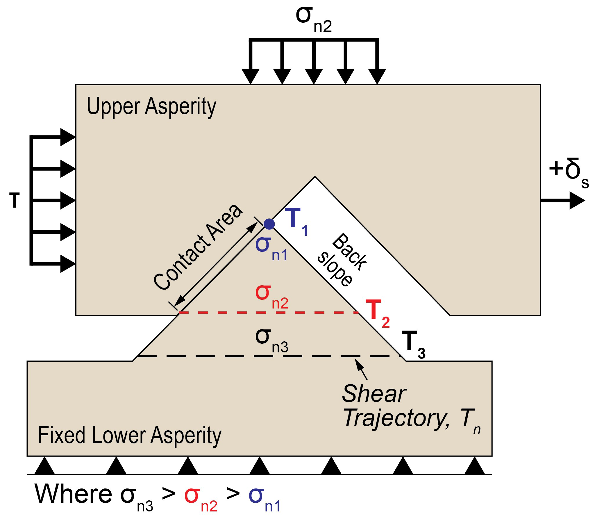
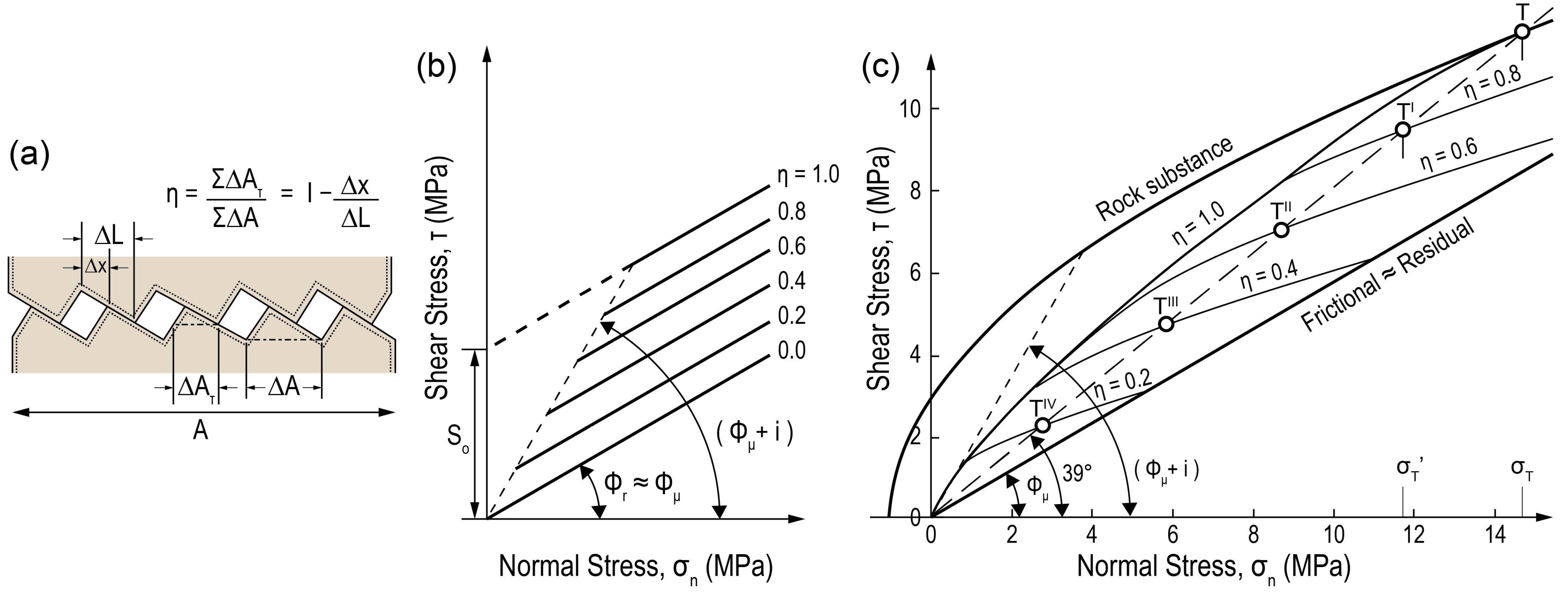
6.2. Shear Failure Mechanism of Rock Fractures

It is well known that joint roughness and asperities play a key role in the shear behaviour of a joint, so it is important to understand the microscopic shear failure mechanism of joints at the scale of an asperity. The two behavioural modes that control joint shear failure, namely, asperity sliding and asperity shearing, have been experimentally observed to act independently at very low and very high normal stresses (e.g., [53,56]). More commonly, these two failure modes have been observed to act together in combination. As the morphology of a natural rock joint is random and complex, it is difficult to accurately recognize the types of shear failure areas [68].

To simplify the visualization of joint shear failure and asperity contact, each joint can be visualized to contain many triangular asperities using a simplified two-dimensional illustration (Figure 13). In Figure 13, the applied normal stress is represented by σ_ni. Depending on the shear direction, only a subset of an asperity will be in contact and subject to surface wear, whereas the back slope of an asperity will not be in contact and can be assumed to have a tensile strength of zero for noncemented joints [44]. The shear mechanism of a joint will vary depending on the applied normal load, strength, and roughness. According to Li et al. [68], the microscopic shear failure mechanism of a joint can be generally explained by the following three trajectories (T_n):

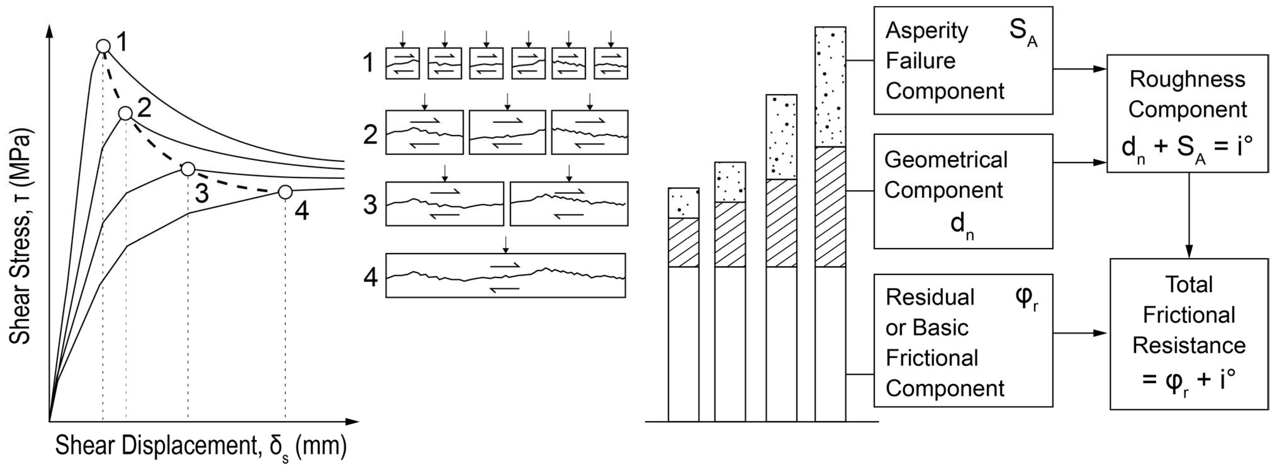
• T₁: Under a low normal stress condition (σ_n1), the upper asperity will slip along the lower asperity to vertex T₁, where major sliding movements occur along the joint. At this point, the shear strength satisfies the lower portion of Patton’s [53,56] bilinear failure envelope, and failure modes of the joint are mainly caused by asperity sliding wear.
• T₃: Under a high normal stress condition that exceeds the strength of intact material of the asperity (σ_n3), no sliding movement occurs, and the asperity is completely sheared through along trajectory T₃. At this point, the shear strength satisfies the upper portion of Patton’s [53,56] bilinear failure envelope, and the failure modes of the joint are mainly caused by shearing through the asperities.
• T₂: Under moderate normal stress conditions that fall in between σ_n1 and σ_n3 (σ_n2), a combination of the two failure modes is expected. Initially, sliding of the upper asperity will occur whereby the sliding shear stress along the asperity is less than the asperity strength. As the sliding continues, the contact area of the joint gradually reduces, and the effective normal stress gradually increases. Thus, the sliding shear stress of the asperity also gradually increases. At some point, the normal stress in the asperity reaches a critical value where the sliding shear stress is greater than the strength of the asperity, and the behaviour will change from sliding to shear failure along trajectory T₂. The failure modes of joints for this scenario are composed of asperity sliding wear and asperity shearing failure.

7. Geomechanical Parameters Calculated from Direct Shear Test Data

In addition to determining the overall shear behaviour of a joint from laboratory direct shear tests, several geomechanical parameters can be calculated from their results. These parameters are in turn used in geomechanics numerical modelling software where joints are discretely simulated for the purpose of rock engineering design. The frequently used geomechanical parameters and the corresponding methods in calculating them from direct shear test data, including pre-peak normal and shear stiffness, yield and peak shear strengths, peak shear displacement, peak friction angle, dilation, and residual shear strength, are presented in the following sections.

7.1. Pre-Yield Deformation Behaviour: Stiffness

Joint deformation is a critical component in understanding joint behaviour and the performance of a discontinuous rock mass under changing stress conditions. To understand joint behaviour, Goodman et al. [3] note that it does not only depend on the applied loads and constraints, but also the properties of component joints (stiffness and strength) along with the fabric of a joint system as a whole (spacing, orientation, persistence, etc.). This section details two of the three component joint parameters that Goodman et al. [3] introduced to describe joint behaviour: joint normal stiffness (K_n) and joint shear stiffness (K_s). These stiffness parameters can be characterized using normal stress versus normal displacement and shear stress versus shear displacement plots by describing the rate of change between normal stress and normal displacement, and shear stress and shear displacement, respectively.

7.1.1. Joint Normal Stiffness (K_n)

Joint normal stiffness is defined as the deformation (joint closure) of a discontinuity that occurs as it is subject to increasing normal stress and can be measured during the initial normal loading stage of a laboratory direct shear test. Experimental results have shown that this relationship can vary and has led to the development of multiple closure laws in order to estimate joint normal deformation (e.g., [20,31,64,69,70,71]). Of these closure laws, the relationship has commonly been described as nonlinear hyperbolic (e.g., [20,64]) and as linear responses (e.g., [31]), and less commonly described as nonlinear power law [70] and semilogarithmic [71,72] responses.

The hyperbolic response has been discussed to be the result of increasing contact areas as normal stress increases. The contact area of a joint when subject to a normal load of zero is very small and is defined by the contacts of a few asperities. When subject to an increasing normal load, the point contacts enlarge by elastic deformation, crushing, and tensile cracking, while the deformation brings new regions into contact [20]. An example of a hyperbolic response is shown in Figure 14a. Along with initial contact area, normal deformability of a discontinuity is also dependent on rock type, joint wall strength, roughness, strength, and deformability of asperities, thickness and properties of infill material (if present), and aperture distribution [64].

In contrast to the hyperbolic response, a linear relationship was found to exist between normal displacement and normal stress in a study completed by Hungr and Coates [31] on natural joints in limestone and sandstone. From the results of their study, it was determined that no correction was needed to be applied to the joint normal closure test results, and neglecting minor irregularities, all normal stress versus normal displacement plots were close to linear. Based on these findings, it was considered realistic to represent the normal stiffness coefficient by fitting a linear function to the plotted results. Further, as the relationship observed differed from those made by [20,69], it was believed that this may be a result caused by the samples of natural joints having been precompressed in situ by pressures considerably greater than those applied in the laboratory tests. Therefore, it is thought that the relationship given by [20,69] is only valid for joints that are not precompressed. Figure 14a outlines the effect that precompression has on the normal stress–displacement behaviour of unfilled joints [31].

The linear relationship observed by Hungr and Coates [31] faced criticism by Bandis et al. [73] as they believed that the observations were a result of three things. First, the joints were subject to previous in situ compression under higher stresses than those used for testing. Second, the applied normal stresses did not range high enough to reveal complete joint behaviour (the maximum applied normal stress in the study by Hungr and Coates [31] was 2.3 MPa). Third, the authors seemingly did not consider the inevitable disturbance of the natural in situ closure seating condition [73].

Swan [70] advised that a power law would be suitable for normal stresses below 30 MPa. Packulak et al. [74] reported good agreement with fitting Swan’s [70] power law to direct shear test data of granitic joints after correcting the test data to eliminate the effect of machine deformation on the fracture deformation results.

Regarding the semilogarithmic closure law, Evans et al. [71] defined its single free parameter as the “stiffness characteristic”, dK_n/dσ_n, which makes this closure law appealing because only one closure measurement over a small normal stress range is needed to fully define the nonlinear stiffness behaviour for a large stress range [72].

Several laws and equations have been developed in efforts to describe joint normal deformability (stiffness). As such, each individual closure law has been developed while considering various assumptions and constraints, and each closure law is subject to a series of advantages and disadvantages. There is currently no recommended normal closure law to be used when evaluating joint normal stiffness according to ASTM Standards and ISRM Suggested Methods [2,9]. Therefore, the selection of a closure law may require the comparison of several closure laws for a dataset in order to determine which law will best represent joint closure for different lithologies and joint characteristics.

7.1.2. Joint Shear Stiffness (K_s)

Joint shear stiffness can be characterized using the shear stress versus shear displacement plot obtained from a direct shear test. Shear stiffness represents the resistance of the specimen to shear displacement under an applied shear force prior to reaching the peak shear strength [9]. Observing the pre-peak portion of a shear stress versus shear displacement plot, both linear and nonlinear behaviours can be identified, with nonlinearity being more profound in weathered and/or disturbed joints. In addition to the degree of weathering, there are several other parameters that affect shear deformability, which include roughness, size, applied normal stress, infill material(s) (if present), and stress history [73]. As the shear load–deformation curves have been observed to be characteristically different, Goodman [75] made several generalizations about the results for different types of weakness surfaces and classified the shear load–deformation curves into four types, as illustrated in Figure 15.

Another factor potentially affecting the peak shear stiffness of a joint is its past in situ loading history [73]. In Barton’s [5] study, a series of direct shear tests were completed on model joints that were both precompressed and normally loaded. The results of these tests demonstrated that precompressed joints (normally loaded to a stress higher than that during the direct shear test) have the potential for a higher shear strength than joints normally loaded. This effect is referred to as “overclosure” and its impact can be observed in Figure 14b.

Despite this natural variability in the behaviour, joint shear stiffness is most often characterized as the slope of the linear elastic region for a shear stress versus shear displacement plot [20]. The characterization of shear stiffness using a linear approach is commonly completed using two methods: (i) the peak (secant) method and (ii) the yield (tangent) method. Additional linear shear stiffness measurement methods are discussed in the following sections, including Day’s [6] best-fit chord and Grasselli and Egger’s [44] method. Nonlinear methods are available in the literature but are not discussed in this study; readers are referred to the following references for additional information on characterizing shear stiffness for nonlinear responses (among others [31,73,76]).

Peak Secant Method

The peak secant method is the most common and simplest approach to measuring shear stiffness of a joint. It is completed by measuring the secant between zero shear stress and the unconstrained peak shear strength on a shear stress–displacement plot, as shown in Figure 2. This method is rather limited as there is no consideration of the influence of sample seating in the nonlinear portion near the beginning of the test, or nonlinear behaviour that may occur immediately prior to reaching unconstrained peak shear strength [6,32,75].

Yield Tangent Method

The second approach is referred to as the yield (tangent) method. This method results in two shear stiffness values through the identification of two characteristic points on a shear stress versus shear displacement plot: (i) the “yield” point, which is defined as the point of maximum curvature, and (ii) the shear stress point at which 50% of unconstrained peak shear strength occurs. Using the two identified points, the tangent of each point can be taken to represent the shear stiffness, or, in the case of a multi-stage direct shear test, where several shear stages are completed on a joint specimen, a “secant coefficient” can be calculated at the critical points for each stage. Using the various secant coefficients, a linear regression analysis can be applied to the data with the “best fit line” crossing through the origin, making the regression coefficient equal to the shear stiffness of the joint [31].

Of these two approaches, it is most common to measure the shear stiffness as the tangent at 50% of unconstrained peak shear strength, which can be approximated by the chord of the curve between 40% and 60% of the unconstrained peak shear strength (Figure 2a). This is an easily repeatable and objective measurement; however, in some cases, using a chord measurement between 40% and 60% of unconstrained peak shear strength may include deviations from an elastic trend, potentially resulting in an inaccurate measurement of shear stiffness [6,32].

Best-Fit Chord Method

The inclusion of nonlinear portions of a shear–displacement curve when measuring shear stiffness will result in an artificially low joint shear stiffness value. In efforts to overcome the noted limitations that come with the peak and yield tangent methods, Day [6] proposed a best-fit chord method to measure the shear stiffness of a joint. The best-fit chord method requires manual selection of the linear elastic portion of a shear stress–displacement curve between the onset of shearing and unconstrained peak shear strength (Figure 2). This technique minimizes the influence of nonlinear behaviour that commonly occurs early in the test and immediately before unconstrained peak shear strength is achieved [6,32].

Although the peak secant and yield tangent methods face limitations, both methods are simplistic and can be determined with consistency by practitioners. Contrary to this, the method proposed by Day [6] is subjective and requires manual selection of the linear region to be measured. This will inevitably introduce variation between practitioners and may result in inconsistent measurements of the same data by different individuals.

Grasselli and Egger Linear Relationship

Grasselli and Egger [44] proposed a linear relationship to define shear stiffness, stating that the nonlinearity observed at the beginning of a shear strength versus shear displacement plot is the result of joints not being entirely mated. This results in a small displacement occurring prior to the joint being able to provide its entire strength. Thus, Grasselli and Egger [44] expressed the shear displacement as the sum of two components: (i) the horizontal displacement necessary to mate the joint (${\delta }_m$) and (ii) the horizontal displacement prior to reaching unconstrained peak shear strength (${\mathsf{\Delta }\delta }_p$). The total horizontal displacement is expressed by Equation (11). Observing the experimental curves as the joint is mated, Grasselli and Egger [44] affirmed that the joints deformed almost linearly up to unconstrained peak shear strength and described shear stiffness using the linear relationship expressed by Equation (12).

$${\delta }_p={\delta }_m+{\mathsf{\Delta }\delta }_p$$

(11)

$$K_s=\frac{1}{{\mathsf{\Delta }\delta }_p}\ast \frac{{\tau }_p}{{\sigma }_n}$$

(12)

7.2. Yield, Unconstrained Peak, and Constrained Peak Shear Strengths

Yield and peak shear strength of a joint are commonly used interchangeably and can therefore be misleading to the reader. In Hungr and Coates’ [31] study, yield is referred to as the point of maximum curvature on a shear stress–displacement curve and the peak shear strength is the maximum shear stress achieved, whereas Goodman [75] refers to the point of maximum curvature as the peak and the yield is undefined.

Depending on the nature of the rock, testing procedures, and other factors, the observed shear response of a joint can take on the form of ductile, semiductile, or brittle behaviour. In the case of these three behaviours, the points of maximum curvature and peak shear strength may vary. Commonly, under CNL* boundary conditions, the unconstrained peak shear strength and yield point coincide for semiductile and brittle behaviour. Conversely, for direct shear tests under CNS conditions, the maximum attainable shear stress may vary from the point of maximum curvature due to a post-peak “strengthening” behaviour [20]. When comparing CNL* and CNS testing, shear behaviour is similar prior to the point of maximum curvature but will diverge after this point. This is the result of an increase in the applied stress under CNS conditions as the sample begins to dilate. Consequently, as the normal stress increases, a higher shear stress will be required to horizontally displace the joint, thus yielding an increase in shear strength. Figure 16 illustrates the shear stress–displacement response for a typical rock joint specimen under CNL* testing conditions (solid lines) and under CNS testing conditions (dashed lines).

Barton et al. [59] state that the variations in these behaviours are a result of scale effect and joint surface properties, where the peak-residual behaviour is a typical representation of small block sizes, rough joints, and low ratios of σ′_n/JCS, whereas the smooth hyperbolic behaviour is a result of large block sizes, smooth joints, and high ratios of σ′_n/JCS.

In the case of multi-stage direct shear testing, the response of a joint may change from an initially brittle response to a ductile shear response. This change can be explained by the shearing of microscopic roughness on the contact areas. In the case of multi-stage testing with repositioning, the contact areas are subject to wear and may be smoothed by the last test stage, creating a different response than stage 1. This occurrence was observed by Grasselli and Egger [44] and MacDonald [19], who continuously sheared a specimen at the same normal stress and observed the shear strength tend towards the same residual value with each subsequent stage (Figure 17). As a result, joints that originally demonstrate brittle behaviour will have a clear peak resistance in the first stage, but for subsequent stages, the occurrence of peak may be difficult to distinguish. The authors of this review recommend that unconstrained peak shear strength be referred to as the maximum attainable shear stress that occurs shortly after yield and is followed by the first decrease in shear stress. Constrained peak shear strength should be referred to as the maximum sustained shear stress that may be observed at shear stresses greater than the unconstrained peak shear strength after additional shear displacement, as often observed with testing under CNS boundary conditions where an increase in the applied normal stress occurs with increasing dilation. Yield shear strength should be used to represent the point of maximum curvature (Figure 2).

7.3. Unconstrained and Constrained Peak Shear Displacements

Unconstrained and constrained peak shear displacements $({\delta }_{p-u}\&{\delta }_{p-c})$ are referred to as the horizontal displacements required to reach unconstrained and constrained peak shear strengths, respectively, and are defined in Figure 2. Unconstrained peak shear displacement is commonly used to determine the secant shear stiffness of a fracture, as previously described in Section 7.1.2. An earlier study completed by Barton [77] indicated that for model tension fractures representing prototype joint lengths from 225 cm up to 2925 cm, it requires approximately 1% of horizontal displacement to reach unconstrained peak shear strength. Despite presenting a 1% “rule of thumb”, Barton and Choubey [4] pointed out that unconstrained peak shear displacement will reduce to less than 1% of joint length as the joint length (L) increases to several meters. An extensive review of 650 in situ and laboratory tests for filled discontinuities, rock joints, and modelled joints by Barton and Bandis [40] provided further evidence to support the observation that as joint length increases, $\frac{{\delta }_{peak}}{L}$ decreases.

7.4. Peak Friction Angle (ϕ)

Peak friction angle (${\varphi }_p$) is commonly measured by one of two ways: (i) calculated using Equation (13) or (ii) measured graphically as the inclination of the linear Mohr–Coulomb failure envelope of a rock joint.

$${\varphi }_p={tan}^{-1}\left(\frac{{\tau }_{p-u}}{{\sigma }_n}\right)$$

(13)

In early work completed by Patton [53], it was concluded that the shearing of a joint exhibits two modes of failure that are best represented by one bilinear failure envelope. The lower part of the envelope is defined by sliding behaviour of the joint, and the upper portion of the envelope is defined by a shearing behaviour. For the lower part of the envelope, the friction angle is the sum of two components: (1) the basic friction angle and (2) the mean inclination of the roughness surface. Although this simple change in failure mode depicted by the bilinear failure envelope is representative for direct shear tests on controlled sawtooth specimens, failure envelopes for natural irregularities will not reflect such a simple change in failure modes; rather, failure modes are expected to occur simultaneously at different intensities [56]. Therefore, under a given normal stress, complete or partial damage of asperities contributes a shearing or failure component ${(S}_A^{°})$ to the peak frictional resistance (${\varphi }_p$). To better represent peak friction angle, a three-component equation was developed instead of two, consisting of (1) the basic friction angle (${\varphi }_b^{°}$), (2) the angular component described in terms of peak dilation ($d_n^{°}$), and (3) the shearing failure component, shown empirically by Equation (14) and graphically in Figure 18 [5,65].

$${\varphi }_p=peak{tan}^{-1}\left(\frac{\tau }{{\sigma }_n}\right)={\varphi }_b^{°}+d_n^{°}+S_A^{°}$$

(14)

7.5. Dilation ($\psi$)

Dilation is a very powerful phenomenological parameter of shear strength, as for a given normal stress it represents the minimum energy path between a sliding and shearing mode of failure [5]. Further, dilation is an important feature when evaluating joint shear strength as it can increase the shear resistance of a discontinuity in one of two ways. Firstly, if a discontinuity is confined, as it begins to dilate it will result in an increase in the applied normal stress, which in turn increases the shear strength. Secondly, as demonstrated in Patton’s [53] work, sliding asperities can increase the frictional resistance by an angle of asperity inclination, i [20]. When shearing of a nonplanar joint occurs, asperities on the joint surface will slide over each other and cause an increase in the aperture (displacement perpendicular to the joint), which is referred to as dilation ($\psi$) [59]. Dilation can be calculated using the instantaneous inclination from a normal displacement versus shear displacement plot by following Equation (15).

$$\psi ={tan}^{-1}\left(\frac{{\delta }_n}{{\delta }_h}\right)$$

(15)

Dilation is known to initialize at an increasing rate as unconstrained peak shear strength is approached and thereafter continuing at a reduced rate as roughness is gradually destroyed [59]. The dilation angle of a fracture depends on the strength of the rock material, angle of asperities, and applied normal stress [3]. The impacts that normal stress and joint roughness have on the dilation angle are illustrated in Figure 19. In general, as the friction of a joint increases, an increase in dilation can be expected, and as the ratio of applied normal stress to joint compressive strength decreases, an increase in dilation will also occur. The inverse relationship observed between dilation angle and applied normal stress has been additionally confirmed by other researchers (e.g., [7,19,20,21,32,78]).

Ultimately, joint characteristics will control the degradation and dilation that a joint will experience during shear. A rough weak joint will suffer greater damage than a strong smooth joint surface, yet neither will experience high degrees of dilation. Strong joints with a high degree of surface roughness will dilate strongly as unconstrained peak shear strength is approached [4]. It has been shown by Barton [79] that the occurrence of the maximum dilation angle corresponds with the shear displacement at which peak strength occurs.

7.6. Residual Shear Strength (τ_r)

Under CNL/CNL* boundary conditions, following unconstrained peak shear strength, a very rapid decrease of strength is often observed on a shear strength versus shear displacement plot, and as the shear displacement continues, the reduction rate of shear strength will slow until it reaches its final value, which is referred to as residual shear strength [80]. True residual strength is said to only be achieved once dilation ceases. As a result, it is difficult to achieve true residual strength, as roughness tends to continuously contribute to shear strength even after large displacements [66]. Barton [5] claims that when testing joints in strong rock, true residual strength will seldom be attained unless the normal stresses are very high, or repeated tests are made. The slow reduction towards residual strength found in practice has prompted the use of a more appropriate definition, termed “ultimate” strength, to represent the value measured at the end of a shear test [66].

Some discrete geomechanics numerical modelling software require that post-peak shear strength be defined by dilation angle, residual shear strength, and maximum dilation. Packulak et al. [7] proposed a measurement method to holistically measure all three of these parameters from direct shear test data. Readers are referred to [7] for details.

Under CNS boundary conditions, following unconstrained peak shear strength, the decrease in shear strength is dampened by the increase of applied normal stress to maintain the input KNM condition. After some amount of shear displacement past unconstrained peak shear strength, which depends on the rock and joint properties and test conditions, constrained peak shear strength will be reached, followed by a very rapid decrease of strength. After further shear displacement, residual shear strength will be achieved (Figure 2).

8. Critical Assessment of Boundary Condition Selection

The decision to test rock fractures in direct shear under a CNL/CNL* or a CNS boundary condition should be evaluated against the environment in which the project of interest is located and the intended use of the laboratory test data. In cases where the normal load/normal stress applied to the discontinuity is expected to remain constant (e.g., rock slope and surface excavation stability or the sliding of structures on rock foundations), direct shear testing under a CNL/CNL* boundary condition is recommended. In rock engineering, there are many instances where the normal stress on a discontinuity would not remain constant as sliding occurs, such as fractures compressed by rock bolts, displaced blocks around an underground excavation, or shearing of joints during fluid injection activities. Fluid injection activities include hydraulic fracturing for petroleum resource extraction or rock mass preconditioning, and carbon dioxide for deep underground sequestration, among others.

Both CNL/CNL* and CNS boundary conditions measure the stiffness, strength, and dilation of the discontinuity, and the current ISRM suggested method states that testing should be completed using a minimum of three (3) but preferably five (5) distinct normal stress conditions. These normal stresses should reflect the expected normal stress that the discontinuities will be subjected to in a given project context. For instance, in the case of the evaluation of the stability and sliding potential of a water-control structure founded on a bedded limestone with an expected load of 300 kPa, a single-stage program consisting of three to five specimens, tested at normal stresses of 100, 200, 300, 400, and 500 kPa under CNL* conditions, would be considered sufficient to determine the strength envelope of the investigated discontinuity set.

The fundamental difference between the CNL/CNL* and the CNS boundary condition is the stress path of the discontinuity during shear. The CNL/CNL* boundary condition holds the applied, normal load/normal stress constant. The CNS boundary condition does not hold the applied normal stress constant; therefore, it is hypothesized that the stress path the discontinuity takes as shearing progresses would be along the strength envelope. As the stress path is believed to follow the strength envelope, hypothetically fewer tests would be required to predict the strength envelope [49]. Furthermore, the direction of the stress path is thought to provide insight as to the orientation of the development of subsequent shear planes [81]. One of the limitations of using the CNS stress path to determine the strength envelope is the degradation of asperities with increasing shear. As the shear displacement increases, asperities will break and the mobilized resistance to shear will decrease until the joint reaches a residual strength state [66,82]. While highlighting the degradation of roughness with increasing shear, CNS conditions provide static strength measurements that are roughly equivalent to the measurement points for CNL/CNL* boundary condition direct shear tests [7].

The dilative properties of rock joints have impacts on the overall rock mass behaviour both on surface and in underground settings. Recall that in underground settings the dilation potential of a rock joint and the confinement of underground environments results in a higher shear resistance [35,83]. However, the dilation potential also impacts the hydraulic conductivity of the joint and the rock mass if fractures are continuous. The study of the evolution of joint permeability with increased shear displacement has been undertaken by numerous researchers, including Archambault et al. [84], Nguyen and Selvadurai [85], Esaki et al. [86], Hans and Boulon [87], Min et al. [88], Barton [89], and Li et al. [90]. These studies show that as the rock joint undergoes shear and the area of contact on the joint plane decreases, water conductivity increases until maximum dilation is reached, or the dilatancy rate becomes zero. In cases where permeability around underground structures is important, such as underground reservoirs for carbon dioxide sequestration and deep geological repositories for the safe storage of spent nuclear fuel, the dilative behaviour of the joint under a CNS boundary condition becomes critical, and CNL/CNL* testing does not accurately capture the increased dampening of the dilation angle due to the increase in normal stress.

9. Critical Assessment of Multi-Stage Direct Shear Testing

Multi-stage direct shear testing has proven to be a useful technique as it can increase the amount of information gained from a single rock specimen, overcome sampling issues when more than one discontinuity cannot be obtained, and limit the natural variability of rock properties in the case of heterogeneous rock specimens. Given these benefits, multi-stage testing has become a common practice in the industry, but it does come with limitations. The impact that multi-stage direct shear testing has on the unconstrained peak shear strength values of subsequent shear stages has not passed unnoticed. Currently, both the ASTM standard and ISRM suggested method contain cautionary statements with the use of multi-stage testing. They read as follows:

• “To minimize the influence of damage and wear, each consecutive shear stage should be performed with an increasingly higher normal stress” [2];
• “In the case of multi-stage tests, the apparent cohesion can be exaggerated due to accumulation of damage with successive shearing of the same joint specimen” [2];
• “In order to reduce the potential for the effects of specimen degradation and wear, each consecutive stage should be performed with a higher normal load… Bear in mind that with each repetition the surface will be further damaged” [9].

The degradation of a specimen’s surface when subject to multiple shear stages has been observed to impact the results since the earliest tests completed on joints and separated bedding planes of sandstone, siltstone, and shale by Ripley and Lee [17]. This observation was later confirmed in a study by Hencher and Richards [91] on sheeting joints in Hong Kong granite, who noted that when using a multi-stage technique, true peak strength was only obtained for the initial stage, and all subsequent stages exhibited a reduced shear strength in comparison to undamaged peak strengths. Despite these initial observations, the use of multi-stage testing persists, and additional research has been carried out to evaluate the feasibility of the testing technique.

In general, direct shear testing will result in surface damage through asperity sliding and shearing. When conducting a multi-stage test, rock specimens are subject to large displacements and the damage will accumulate with each stage, thus changing the overall surface morphology of a sample and resulting in lower shear strength results for the later stages than might be expected with an undamaged surface. This issue has been addressed by many researchers (among others, [11,12,13,14,15,16,17,18,19,91,92]). Figure 17 illustrates the reduction in shear strength of a specimen that is sheared multiple times and repositioned after 5 mm of displacement under the same normal load for each stage [44]. In specimens with rougher surface profiles, it is suggested that shear forces accumulate on the irregular sample surface against the highest asperities, reaching larger intensities [93]. Therefore, damage typically concentrates on one or a few dominant asperities. In cases where only a few asperities play a role, test-induced damage will have a significant impact on the shear strength observed in subsequent stages of a multi-stage test, as in the later stages, dominant asperities may be absent through damage and may be controlled by less prominent asperities [94].

The same occurrence In shear strength reduction can be observed when a specimen is tested following a multi-stage procedure without repositioning. In addition to surface damage, the lack of interlocking between asperities as shear displacement progresses contributes to lower shear strengths. This occurrence was empirically demonstrated and confirmed experimentally on ordinary compressed concrete bricks by Ladanyi and Archambault [21], who noted “for an increasing loss of interlock, the maximum strength is seen to tend more and more to the residual one”. To visualize the reduction in unconstrained peak shear strengths as a result of decreasing levels of interlocking asperities, Ladanyi and Archambault [21] published their results compared to Patton’s [53,56] shear behaviour constitutive models (Figure 20). Ladanyi and Archambault’s [21] model includes the definitions of transition stress points (σ_T) along a linear slope of 39° [95,96], at points T^I–IV in Figure 20c, because at normal stresses exceeding the transition stresses, the strength envelopes for discontinuities would join the one for rock mass because the discontinuities would have little effect on the strength of the rock mass.

Experimentally, the impact that multi-stage testing without repositioning has on the unconstrained peak shear strength of concrete lift joints sorted by corresponding shear stage is illustrated in Figure 21 [17]. Here, there is a clear reduction in both cohesion and friction angle of the failure envelopes between shear stages 1 to 5.

More recently, Gaines [18] completed a study on tension-induced Saint-Canut sandstone joints that confirms previous findings and expands on the comparison of multi-stage testing with and without repositioning. He concluded that multi-stage testing without repositioning is far more inaccurate than multi-stage testing with repositioning. In agreement with Ladanyi and Archambault [21], Gaines [18] believes the decrease in apparent shear strength is likely due to the lack of interlocking of asperities and minor undulations as shear displacement progresses. A visual summary of the results from Gaines’ [18] study is provided in Figure 22.

When combining the results from damaged and undamaged surfaces, an underestimation in friction and overestimation in cohesion can be expected when defining Mohr–Coulomb parameters [12,16,17,18,19]. This problem is accentuated when a sample has a high JRC, low JCS, and the applied normal stress is high in relation to JCS, therefore causing more damage during each stage [16]. Figure 23 illustrates this occurrence, where “standard” refers to a multi-stage direct shear test with repositioning, as described by ISRM and ASTM, beginning at the lowest normal stress and ascending to the highest.

In the study completed on sheeting joints in Hong Kong granite by Hencher and Richards [91], it was suggested that when significant losses of peak strength are suspected, the effect may be quantified by testing similar samples under decreasing normal stresses. This allows for a comparison of the maximum shear strengths achieved at the highest normal load to see if the sample loading history has an impact on the results. To overcome the issue of (false) unconstrained peak shear strengths measured from multi-stage tests, Hencher and Richards [13,14] note that when conducting multi-stage direct shear tests, it is good practice to carry out tests with different normal loads for the first stage, so the first-stage results can be used by themselves to define the unconstrained peak shear strength envelope if necessary. This testing philosophy was carried out in two direct shear testing programs by Yathon et al. [17] and Gaines [18]. When applying this approach, the results demonstrate that the selection of the initial normal stress along with the magnitude of normal stress increase between each stage will impact the interpreted Mohr–Coulomb shear strength properties [18]. Figure 24 contains the results of multi-stage direct shear tests completed on concrete lift joints by Yathon et al. [17]. This demonstrates how interpreted shear strength properties can vary depending on whether the stages of applied normal stress follow an ascending or descending order. The slope and intercept of the linear regression will be influenced by the first-stage results as it is performed on an undamaged surface [17].

To overcome the issue of excessive asperity damage due to large shear displacements, the LDMDS was proposed [11,12]. This recently developed testing technique has been observed to minimize asperity damage and provide more accurate peak shear strength parameters compared to conventional multi-stage direct shear tests. These findings were validated through an experimental study using joint replicas made of cement to directly compare the results of LDMDS and single-stage procedures, illustrated in Figure 23 [11].

The recent laboratory investigation completed by Gaines [18] at the Government of Canada’s CanmetMINING Rock Mechanics Laboratory assessed the strength of induced rock joints in sandstone by applying different testing procedures and interpretation methods. Direct shear testing was completed using multi-stage, with and without repositioning, and limited displacement multi-stage procedures to quantify the difference between interpreted strength parameters for each testing method. In agreement with other researchers, each subsequent shear stage in the multi-stage test resulted in a shear stress vs. shear displacement plot containing a poorly defined unconstrained peak shear strength due to asperity damage and is more representative of the residual stress. Based on the test results, it was found that multi-stage testing without repositioning is significantly more inaccurate than multi-stage testing with repositioning. This is believed to be the result of poor asperity interlocking and minor undulations as shear displacement progresses. Furthermore, the results from the limited displacement multi-stage tests contain better agreement with the undamaged results and more accurately estimate strength parameters [18].

10. Concluding Remarks

Direct shear testing is a common laboratory method used to measure geomechanical properties of rock discontinuities, dating back to the 1950s. Currently, common practice includes three boundary conditions, namely, constant normal load (CNL), constant normal stress (CNL*), and constant normal stiffness (CNS), and two standardized testing procedures, namely, single-stage and multi-stage direct shear testing.

10.1. Boundary Conditions

CNL and CNL* are presently the most often used boundary conditions for direct shear testing and are considered to represent near-surface rock mass environments where gravity loading dominates rock mass stability. CNL was the first type of direct shear testing with load applied through a mechanical lever arm loaded with metal weights of known mass [91,97]. CNL* can be achieved with servo-controlled hydraulics and computer-programmed laboratory equipment, where the specimen contact area can be automatically calculated throughout the test as shear displacement progresses. In this case, the normal load is proportionately increased during a test as contact area decreases to maintain the preset normal stress magnitude. The results from a CNL* test program are easy to directly input into geomechanics numerical models with discrete joint elements for rock engineering design where normal stiffness, shear stiffness, peak and residual shear strengths, and dilation are required parameters.

The CNS boundary condition is considered to represent deep rock mass environments near underground excavations where ground stresses control rock mass stability. CNS boundary conditions can be achieved in laboratory direct shear tests by adding physical springs of known stiffness to a test system, or by programming a stiffness magnitude into servo-controlled hydraulic equipment. In dry conditions, Packulak et al. [7] demonstrated very similar shear strength results of rough granitic joints between CNL* and CNS boundary conditions. CNS testing is particularly relevant for understanding the evolution of dilation and implications for fracture permeability and fluid flow from initial pre-peak to residual post-peak shear behaviour.

10.2. Multi-Stage Test Procedures

Multi-stage direct shear testing subjects a single specimen to additional shear stages, resulting in subsequent stages being performed on a progressively damaged surface. Thus, the peak shear strength results measured in the subsequent stages result in values that are lower than expected. As such, multi-stage direct shear testing has become a controversial procedure, resulting in several studies being completed to test its validity, which are summarized in

Table 1. Summary of major findings pertaining to multi-stage direct shear testing procedures.

Major Findings/Contributions	References
Suggested carrying out multi-stage direct shear testing programs using a different normal load for the first stage. This allows the results from the first stage to be used by themselves to define peak shear strength envelopes.	[13,14]
Developed an alternative direct shear testing procedure, referred to as the limited displacement multi-stage direct shear test (LDMDS), in efforts to improve multi-stage direct shear testing.	[11,12]
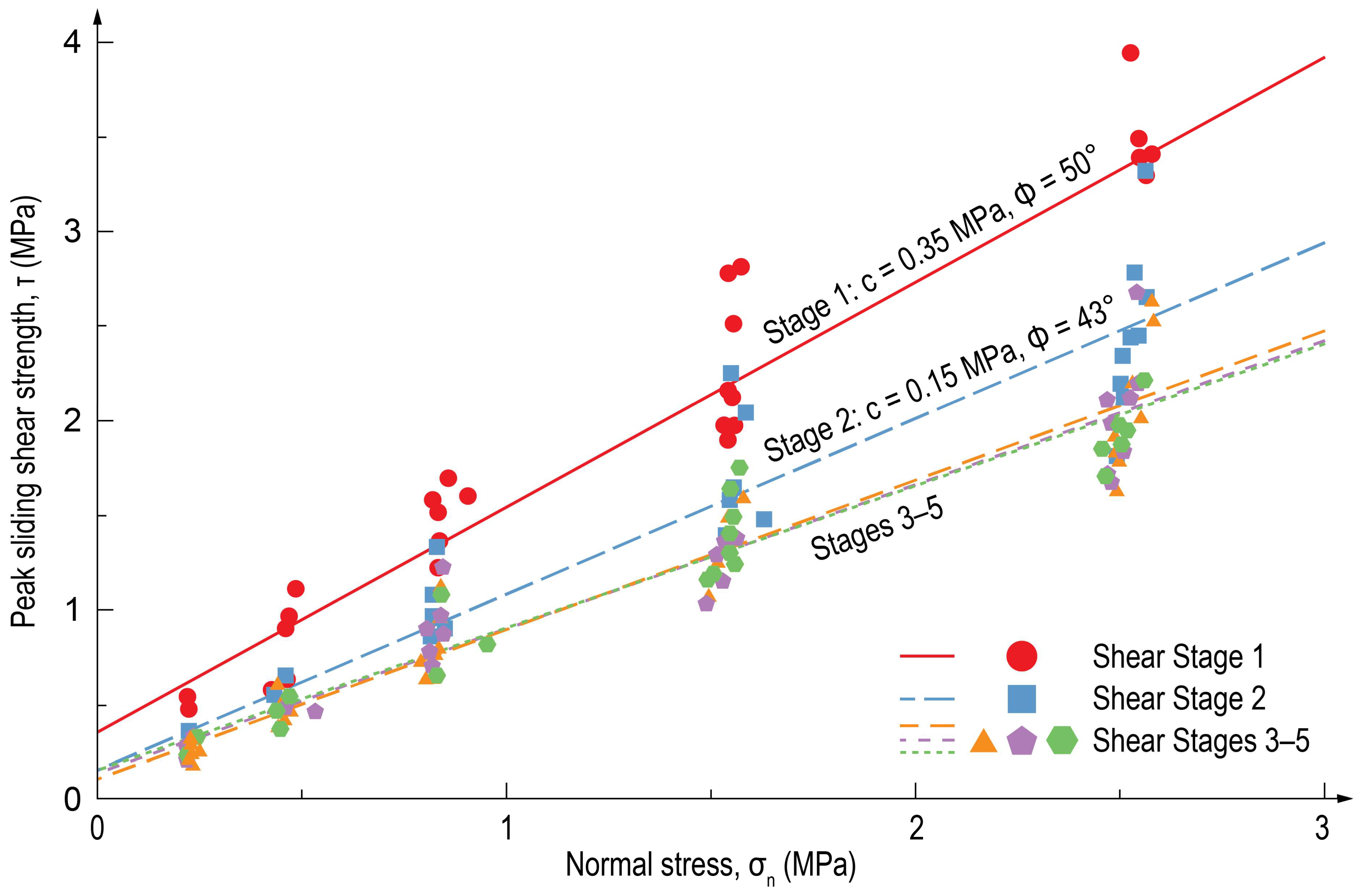
Evaluated the limitations involved with peak shear strength measurements and interpreted shear strength parameters when following a multi-stage direct shear testing procedure with repositioning as published by the ASTM and ISRM. Results demonstrated a decrease in peak shear strength with subsequent stages when compared to single-stage results. This impacts the interpreted Mohr–Coulomb shear strength parameters by overestimating the cohesion and underestimating the joint friction angle.	[11,12,18,19]
Compared the peak shear strength and interpreted Mohr–Coulomb shear strength parameters of LDMDS vs. multi-stage vs. single-stage direct shear testing procedures. Results demonstrated an improvement in defining peak shear strength parameters for LDMDS testing when compared to multi-stage testing and using single-stage results for comparative purposes.	[11,12,18,19]
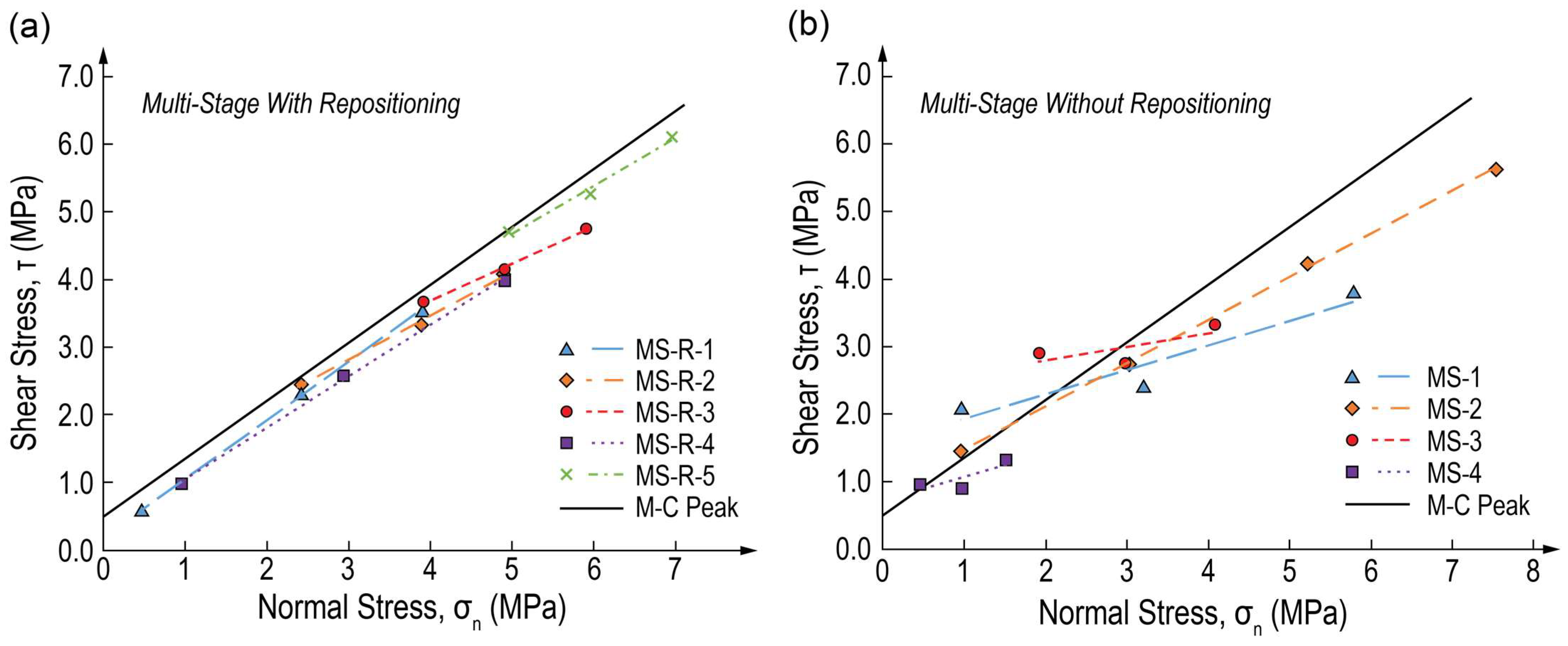
Evaluated the impact on direct shear testing results when following a multi-stage direct shear testing procedure without repositioning as published by the ASTM and ISRM. Results demonstrated that multi-stage direct shear testing with repositioning is far more accurate than multi-stage without repositioning.	[17,18]
Utilized the suggestions from [13,14]. Findings demonstrated that the selection of the initial normal stress along with the magnitude of normal stress increase (or decrease) for each stage will impact the interpreted Mohr–Coulomb shear strength parameters.	[17,18]
When following a multi-stage direct shear testing procedure in a descending order (beginning with the highest normal stress for stage 1 and decreasing with each stage), the interpreted Mohr–Coulomb failure envelope will have a lower cohesion and higher friction angle as opposed to a higher cohesion and lower friction angle when following an ascending order.	[17]

. These studies have shown that when combining multi-stage testing results, and following an ascending order for applied normal stress, the interpreted Mohr–Coulomb shear strength envelope parameters underestimate friction angle and overestimate apparent cohesion.

To overcome this issue, an alternative testing procedure has been introduced that reduces the surface damage experienced by a specimen. This testing procedure is referred to as the limited displacement multi-stage direct shear test (LDMDS). Additional studies have been completed to compare the three testing procedures and conclude that LDMDS is more accurate than multi-stage testing. Despite having shown improvements, of the published studies comparing all three testing procedures, they are limited, as one study only tests specimens at low normal stresses (less than 0.5 MPa) and both studies fail to consider parameters other than peak shear strength and the associated Mohr–Coulomb shear strength parameters. These limitations prompted additional testing by the authors of this review to further investigate the influence that various testing procedures have on laboratory direct shear results subject to high normal stresses and on other geomechanical properties such as joint normal and shear stiffness, joint dilation angles, residual shear strength, and associated failure mechanisms. The results of this experimental study by the authors are forthcoming.

References

1. ISRM; Franklin, J.A.; Kanji, M.A.; Herget, G.; Ladanyi, B.; Drozd, K.; Dvorak, A.; Egger, P.; Kutter, H.; Rummel, F.; et al. Suggested methods for determining shear strength. Int Soc Rock Mech Commission on Testing Methods. In The Complete ISRM Suggested Methods for Rock Characterization, Testing and Monitoring: 1974–2006; Ulusay, R., Hudson, J.A., Eds.; ISRM: Ankara, Turkey, 2007; pp. 165–176. [Google Scholar]
2. Muralha, J.; Grasselli, G.; Tatone, B.; Blümel, M.; Chryssanthakis, P.; Yujing, J. ISRM suggested method for laboratory determination of the shear strength of rock joints: Revised version. Rock Mech. Rock Eng. 2014, 47, 291–302. [Google Scholar] [CrossRef]
3. Goodman, R.E.; Taylor, R.L.; Brekke, T.L. A model for the mechanics of jointed rock. J. Soil Mech. Found. Div. 1968, 94, 637–659. [Google Scholar] [CrossRef]
4. Barton, N.; Choubey, V. The shear strength of rock joints in theory and practice. Rock Mech. 1977, 10, 1–54. [Google Scholar] [CrossRef]
5. Barton, N. Review of a new shear strength criterion for rock joints. Eng. Geol. 1973, 7, 287–332. [Google Scholar] [CrossRef]
6. Day, J.J. The Influence of Healed Intrablock Rockmass Structure on the Behaviour of Deep Excavations in Complex Rockmasses. Ph.D. Thesis, Department of Geological Sciences and Geological Engineering, Queen’s University, Kingston, ON, Canada, 2016. Available online: https://qspace.library.queensu.ca/handle/1974/15306 (accessed on 12 May 2022).
7. Packulak, T.R.M.; Day, J.J.; Diederichs, M.S. Enhancement of constant normal stiffness direct shear testing protocols for determining geomechanical properties of fractures. Can. Geotech. J. 2022, 59, 1643–1659. [Google Scholar] [CrossRef]
8. Barton, N.; Bandis, S.C. Review of predictive capabilities of JRC-JCS model in engineering practice. In Proceedings of the Rock Joints-Proceeding of a Regional Conference of the International Society for Rock Mechanics, Loen, Norway, 4–6 June 1990; pp. 603–610. [Google Scholar]
9. ASTM D5607-16; Standard Test Method for Performing Laboratory Direct Shear Strength Tests of Rock Specimens under Constant Normal Force. ASTM International: West Conshohocken, PA, USA, 2016.
10. Barla, G.; Robotti, F.; Vai, L. Revisiting Large Size Direct Shear Testing of Rock Mass Foundations. In Proceedings of the 6th International Conference on Dam Engineering, Lisbon, Portugal, 15–17 February 2011; p. 10. [Google Scholar]
11. Petro, M. Characterization of Peak Shear Strength of Rough Rock Joints Using the Limited Displacement Multi-Stage Direct Shear (LDMSD) Test Method. Master’s Thesis, Montana Technological University, Butte, MT, USA, 2018. [Google Scholar]
12. MacLaughlin, M.; Berry, S.; Petro, M.; Berry, K.; Bro, A. Characterization of peak shear strength of rough rock joints using limited displacement multi-stage direct shear (LDMDS) tests. E3S Web Conf. 2019, 92, 13011. [Google Scholar] [CrossRef]
13. Hencher, S.R.; Richards, L.R. Laboratory direct shear testing of rock discontinuities. Ground Eng. 1989, 22, 24–31. [Google Scholar]
14. Hencher, S.R.; Richards, L.R. Assessing the shear strength of rock discontinuities at laboratory and field scales. Rock Mech. Rock Eng. 2015, 48, 883–905. [Google Scholar] [CrossRef]
15. Muralha, J. Stress paths in laboratory joint shear tests. In Proceedings of the 11th International Society for Rock Mechanics (ISRM) Congress, Lisbon, Portugal, 9–13 July 2007; Taylor & Francis Group: London, UK, 2007; pp. 431–434. [Google Scholar]
16. Barton, N. Shear strength criteria for rock, rock joints, rockfill and rock masses: Problems and some solutions. J. Rock Mech. Geotech. Eng. 2013, 5, 249–261. [Google Scholar] [CrossRef] [Green Version]
17. Yathon, J.; Chakrabarti, S.; Penner, O.; Lindenbach, E.; Bergman, B.; Razavi-Darbar, S. A novel approach for characterizing shear strength of concrete joints: Experimental procedure and empirical model. In Proceedings of the 39th Annual Conference and Exhibition, Chicago, IL, USA, 8–11 April 2019; p. 14. [Google Scholar]
18. Gaines, S. Interpretation of the peak and residual strength of induced tension fractures in sandstone by single-stage and multi-stage direct shear tests. In Proceedings of the 54th US Rock Mechanics/Geomechanics Symposium, Virtual Event (Physical Event Cancelled), 28 June–1 July 2020. [Google Scholar]
19. MacDonald, N.R. A Critical Laboratory Investigation of Multi-Stage Direct Shear Testing Procedures on Rock Joints Using Synthetic Replica Specimens. Master’s Thesis, Department of Geological Sciences and Geological Engineering, Queen’s University, Kingston, ON, Canada, 2022. Available online: https://qspace.library.queensu.ca/handle/1974/30277 (accessed on 15 August 2022).
20. Goodman, R.E. Methods of Geological Engineering in Discontinuous Rocks; West Publishing Company: St. Paul, MN, USA, 1976; p. 472. [Google Scholar]
21. Ladanyi, B.; Archambault, G. Simulation of shear behavior of a jointed rock mass. In Proceedings of the 11th U.S. Symposium on Rock Mechanics, Berkeley, CA, USA; 1969; pp. 105–125. [Google Scholar]
22. Johnston, I.W.; Lam, T.S.K.; Williams, A.F., Sr. Constant normal stiffness direct shear testing for socketed pile design in weak rock. Géotechnique 1987, 37, 83–89. [Google Scholar] [CrossRef]
23. Lambe, T.W.; Whitman, R.V. Soil Mechanics; Wiley: New York, NY, USA, 1969. [Google Scholar]
24. De Beer, I.E.E. The cell-test. Géotechnique 1950, 2, 162–172. [Google Scholar] [CrossRef]
25. Taylor, D.W. A triaxial shear investigation on a partially saturated soil. In Triaxial Testing of Soils and Bitminous Mixtures; Davis, H.E., Holtz, W.G., Housel, W.S., Eds.; ASTM International: West Conshohocken, PA, USA, 1951; pp. 180–191. [Google Scholar]
26. Jaeger, J.C. The frictional properties of joints in rock. Geofis. Pura Appl. 1959, 43, 148–158. [Google Scholar] [CrossRef]
27. Ripley, C.F.; Lee, K.L. Sliding friction tests on sedimentary rock specimens. In Proceedings of the 7th International Congress on Large Dams, Rome, Italy, 26 June–1 July 1961; pp. 657–671. [Google Scholar]
28. Withers, J.H. Sliding Resistance Along Discontinuities in Rock Masses. Ph.D. Thesis, University of Illinois at Urbana-Champaign, Champaign, IL, USA, 1964. [Google Scholar]
29. Kovari, K.; Tisa, A. Multiple failure state and strain controlled triaxial tests. Rock Mech. Rock Eng. 1975, 7, 17–33. [Google Scholar] [CrossRef]
30. Kim, M.M.; Ko, H.-Y. Multistage triaxial testing of rocks. ASTM Geotech. Test. J. 1979, 2, 98–105. [Google Scholar] [CrossRef]
31. Hungr, O.; Coates, D.F. Deformability of joints and its relation to rock foundation settlements. Can. Geotech. J. 1978, 15, 239–249. [Google Scholar] [CrossRef]
32. Day, J.J.; Diederichs, M.S.; Hutchinson, D.J. New direct shear testing protocols and analyses for fractures and healed intrablock rockmass discontinuities. Eng. Geol. 2017, 229, 53–72. [Google Scholar] [CrossRef]
33. Packulak, T.R.M. Laboratory Investigation of Shear Behaviour in Rock Joints under Varying Boundary Conditions. Master’s Thesis, Department of Geological Sciences and Geological Engineering, Queen’s University, Kingston, ON, Canada, 2018. Available online: https://qspace.library.queensu.ca/handle/1974/24827 (accessed on 1 June 2022).
34. Younkin, G.W. Industrial servo control systems fundamentals and applications. In Revised and Expanded, 2nd ed.; Marcel Dekker Inc: New York, NY, USA, 2003; p. 384. [Google Scholar]
35. Obert, L.; Brady, B.T.; Schmechel, F.W. The Effect of Normal Stiffness on the Shear Resistance of Rock. Rock Mech. 1976, 8, 57–72. [Google Scholar] [CrossRef]
36. Heuze, F.E. Dilatant Effects of Rock Joints. In Proceedings of the 4th International Congress on Rock Mechanics, Montreux, Switzerland, 2–8 September 1979; pp. 169–175. [Google Scholar]
37. Indraratna, B.; Haque, A.; Aziz, N. Shear behaviour of idealized infilled joints under constant normal stiffness. Géotechnique 1999, 49, 331–355. [Google Scholar] [CrossRef]
38. Saeb, S.; Amadei, B. Modelling rock joints under shear and normal loading. Int. J. Rock Mech. Min. Sci. Geomech. Abstr. 1992, 29, 267–278. [Google Scholar] [CrossRef]
39. Skinas, C.A.; Bandis, S.C.; Demiris, C.A. Experimental investigation and modelling of rock joint behaviour under constant stiffness. In Proceedings of the International Symposium on Rock Joints, Loen, Norway, 4–6 June 1990; pp. 301–308. [Google Scholar]
40. Barton, N.; Bandis, S. Effect of block size on the shear behavior of jointed rocks. In Proceedings of the 23rd U.S. Symposium on Rock Mechanics, Berkeley, CA, USA, 25–27 August 1982; pp. 739–760. [Google Scholar]
41. Liu, Q.; Tian, Y.; Liu, D.; Jiang, Y. Updates to JRC-JCS model for estimating the peak shear strength of rock joints based on quantified surface description. Eng. Geol. 2017, 228, 282–300. [Google Scholar] [CrossRef]
42. Plesha, M.E. Constitutive models for rock discontinuities with dilatancy and surface degradation. Int. J. Numer. Anal. Methods Geomech. 1987, 11, 345–362. [Google Scholar] [CrossRef]
43. Homand, F.; Belem, T.; Souley, M. Friction and degradation of rock joint surfaces under shear loads. Int. J. Numer. Anal. Methods Geomech. 2001, 25, 973–999. [Google Scholar] [CrossRef]
44. Grasselli, G.; Egger, P. Constitutive law for the shear strength of rock joints based on three-dimensional surface parameters. Int. J. Rock Mech. Min. Sci. 2003, 40, 25–40. [Google Scholar] [CrossRef]
45. Asadollahi, P.; Tonon, F. Constitutive model for rock fractures: Revisiting Barton’s empirical model. Eng. Geol. 2010, 113, 11–32. [Google Scholar] [CrossRef]
46. Ohnishi, Y.; Dharmaratne, P.G.R. Shear behaviour of physical models of rock joints under constant normal stiffness conditions. In Proceedings of the International Symposium on Rock Joints, Loen, Norway, 4–6 June 1990; pp. 267–273. [Google Scholar]
47. Shrivastava, A.K.; Rao, K.S. Shear behaviour of rock joints under CNL and CNS boundary conditions. Geotech. Geol. Eng. 2015, 33, 1205–1220. [Google Scholar] [CrossRef]
48. Thirukumaran, S.; Indraratna, B. A review of shear strength models for rock joints subjected to constant normal stiffness. J. Rock Mech. Geo. Eng. 2016, 8, 405–414. [Google Scholar] [CrossRef] [Green Version]
49. Haque, A.; Indraratna, B. Experimental and Numerical Modelling of Shear Behaviour of Rock Joints. In Proceedings of the ISRM International Symposium, Melbourne, Victoria, Australia, 19–24 November 2000. [Google Scholar]
50. Bahaaddini, M.; Sharrock, G.; Hebblewhite, B.K. Numerical direct shear tests to model the shear behaviour of rock joints. Comput. Geotech. 2013, 51, 101–115. [Google Scholar] [CrossRef]
51. Nguyen, V.M.; Konietzky, H.; Frühwirt, T. New Methodology to Characterize Shear Behaviour of Joints by Combination of Direct Shear Box Testing and Numerical Simulations. Geotech. Geol. Eng. 2014, 32, 829–846. [Google Scholar] [CrossRef]
52. Coulomb, C.A. Essai sur une Application des Règles de Maximis & Minimis à Quelques Problèmes de Statique, Relatifs à L’architecture; De l’Imprimerie Royale: Paris, France, 1776; Volume 7, pp. 343–382. [Google Scholar]
53. Patton, F.D. Multiple Modes of Shear Failure in Rock and Related and Related Materials. Ph.D. Thesis, University of Illinois, Geology, Champaign, IL, USA, 1966. [Google Scholar]
54. Ghazvinian, A.H.; Azinfar, M.J.; Geranmayeh Vaneghi, R. Importance of Tensile Strength on the Shear Behavior of Discontinuities. Rock Mech. Rock Eng. 2012, 45, 349–359. [Google Scholar] [CrossRef]
55. Yang, J.; Rong, F.; Hou, D.; Peng, J.; Zhou, C. Experimental Study on Peak Shear Strength Criterion for Rock Joints. Rock Mech. Rock Eng. 2016, 49, 821–835. [Google Scholar] [CrossRef]
56. Patton, F.D. Multiple modes of shear failure in rock. In Proceedings of the 1st International Society for Rock Mechanics, Lisbon, Portugal, 25 September–1 October 1966; Volume 1, pp. 509–513. [Google Scholar]
57. Newland, P.L.; Allely, B.H. Volume changes in drained triaxial tests on granular materials. Géotechnique 1957, 7, 17–34. [Google Scholar] [CrossRef]
58. Wyllie, D.C.; Mah, C.W. Rock Slope Engineering: Civil and Mining, 4th ed.; Spon Press: Taylor and Francis Group: New York, NY, USA, 2004. [Google Scholar]
59. Barton, N.; Bandis, S.; Bakhtar, K. Strength, deformation and conductivity coupling of rock Joints. Int. J. Rock Mech. Min. Sci. Geomech. Abstr. 1985, 22, 121–140. [Google Scholar] [CrossRef]
60. Barton, N.; Oslo, A. Details Related to the Ten JRC Profiles and Further Work. Researchgate. 2021. Available online: https://www.researchgate.net/publication/354657828_Details_related_to_the_ten_JRC_profiles_and_further_work (accessed on 25 July 2022).
61. Deere, D.U.; Miller, R. Engineering Classification and Index Properties for Intact Rock; Technical Report No. AFWL-TR-65-116; University of Illinois: Urbana, IL, USA, 1966; p. 327. [Google Scholar]
62. Barton, N.R.; Bandis, S.C. Characterization and modelling of the shear strength, stiffness and hydraulic behaviour of rock joints for engineering purposes. In Rock Mechanics and Engineering Volume 1, 1st ed.; CRC Press: London, UK, 2017; p. 39. [Google Scholar]
63. Pratt, H.R.; Black, A.D.; Brace, W.F. Friction and deformation of jointed quartz diorite. In Proceedings of the 3rd Congress of the International Society for Rock Mechanics, Denver, CO, USA, 1–7 September 1974; pp. 306–310. [Google Scholar]
64. Bandis, S. Experimental Studies of Scale Effects on Shear Strength, and Deformation of Rock Joints. Ph.D. Thesis, Department of Earth Sciences, University of Leeds, Leeds, UK, 1980. [Google Scholar]
65. Bandis, S.; Lumsden, A.C.; Barton, N. Experimental studies of scale effects on the shear behaviour of rock joints. Int. J. Rock Mech. Min. Sci. Geomech. Abstr. 1981, 18, 1–21. [Google Scholar] [CrossRef]
66. Barton, N. Modelling Rock Joint Behavior from In Situ Block Tests: Implications for Nuclear Waste Repository Design; Technical Report; ONWI-308; Terra Tek Inc.: Columbus, OH, USA, 1982. [Google Scholar]
67. Itasca Consulting Group Ltd. UDEC Version 7.00.77. 2022. Available online: https://www.itasca.ca/software/UDEC (accessed on 14 May 2022).
68. Li, Y.; Song, L.; Jiang, Q.; Yang, C.; Liu, C.; Yang, B. Shearing performance of natural matched joints with different wall strengths under direct shearing tests. ASTM Geotech. Test. J. 2018, 41, 20160315. [Google Scholar] [CrossRef]
69. Goodman, R.E. The mechanical properties of joints. In Proceedings of the 3rd Congress of the International Society for Rock Mechanics, Denver, CO, USA, 1–7 September 1974; pp. 1–7. [Google Scholar]
70. Swan, G. Determination of stiffness and other joint properties from roughness measurements. Rock Mech. Rock Eng. 1983, 16, 19–38. [Google Scholar] [CrossRef]
71. Evans, K.; Kohl, T.; Rybach, L.; Hopkirk, R. The effects of fracture normal compliance on the long term circulation behavior of a hot dry rock reservoir: A parameter study using the new fully-coupled code FRACture. In Proceedings of the Annual Meeting of the Geothermal Resources Council, San Diego, CA, USA, 4–7 October 1992; Volume 16, pp. 449–456. [Google Scholar]
72. Zangerl, C.; Evans, K.F.; Eberhardt, E.; Loew, S. Normal stiffness of fractures in granitic rock: A compilation of laboratory and in-situ experiments. Int. J. Rock Mech. Min. Sci. 2008, 45, 1500–1507. [Google Scholar] [CrossRef]
73. Bandis, S.C.; Lumsden, A.C.; Barton, N.R. Fundamentals of rock joint deformation. Int. J. Rock Mech. Min. Sci. Geomech. Abstr. 1983, 20, 249–268. [Google Scholar] [CrossRef]
74. Packulak, T.R.M.; Day, J.J.; Ahmed Labeid, M.T.; Diederichs, M.S. New data processing protocols to isolate fracture deformations to measure normal and shear joint stiffness. Rock Mech. Rock Eng. 2022, 55, 2631–2650. [Google Scholar] [CrossRef]
75. Goodman, R.E. The deformability of joints. In Proceedings of the Determination of the In Situ Modulus of Deformation of Rock, ASTM STP 477, American Society for Testing Materials Winter Meeting, Denver, CO, USA, February 1969; pp. 174–196. [Google Scholar]
76. Clough, G.W.; Duncan, J.M. Finite Element Analyses of Port Allen and Old River Locks; Contract Report S-69-6; U.S. Army Engineer Waterways Experiment Station: Vicksburg, MI, USA, 1969. [Google Scholar]
77. Barton, N.R. A relationship between joint roughness and joint shear strength. In Proceedings of the Symposium of the International Society for Rock Mechanics and Rock Fracture, Paper I-8, Nancy, France, 4–6 October 1971; p. 20. [Google Scholar]
78. Amadei, B.; Wibowo, J.; Sture, S.; Price, R.H. Applicability of existing models to predict the behavior of replicas of natural fractures of welded tuff under different boundary conditions. Geotech. Geol. Eng. 1998, 16, 79–128. [Google Scholar] [CrossRef]
79. Barton, N.R. A Model Study of the Behaviour of Steep Excavated Rock Slopes. Ph.D. Thesis, University of London, London, UK, 1971. [Google Scholar]
80. Krsmanović, D. Initial and Residual Shear Strength of Hard Rocks. Géotechnique 1967, 17, 145–160. [Google Scholar] [CrossRef]
81. Johnston, I.W.; Lam, T.S.K. Shear Behaviour of Regular Triangular Concrete/Rock Joints—Analysis. J. Geotech. Eng. 1989, 115, 711–727. [Google Scholar] [CrossRef]
82. Gentier, S.; Riss, J.; Archambault, G.; Flamand, R.; Hopkins, D. Influence of fracture geometry on shear behaviour. Int. J. Rock Mech. Min. Sci. 2000, 37, 161–174. [Google Scholar] [CrossRef]
83. Pender, M.J. Prefailure Joint Dilatancy and the Behaviour of a Beam with Vertical Joints. Rock Mech. Rock Eng. 1985, 18, 253–266. [Google Scholar] [CrossRef]
84. Archambault, G.; Gentier, S.; Riss, J.; Flamand, R. The evolution of void spaces (permeability) in relation with rock joint shear behaviour. Int. J. Rock Mech. Min. Sci. 1997, 34, 14.e1–14.e15. [Google Scholar] [CrossRef]
85. Nguyen, T.S.; Selvadurai, A.P.S. A model for coupled mechanical and hydraulic behaviour of a rock joint. Int. J. Numer. Anal. Meth. Geomech. 1998, 22, 29–48. [Google Scholar] [CrossRef]
86. Esaki, T.; Du, S.; Mitani, Y.; Ikusada, K.; Jing, L. Development of a shear-flow test apparatus and determination of coupled properties for a single rock joint. Int. J. Rock Mech. Min. Sci. 1999, 36, 641–650. [Google Scholar] [CrossRef]
87. Hans, J.; Boulon, M. A new device for investigating the hydro-mechanical properties of rock joints. Int. J. Numer. Anal. Meth. Geomech. 2003, 27, 513–548. [Google Scholar] [CrossRef]
88. Min, K.B.; Rutqvist, J.; Tsang, C.F.; Jing, L. Stress-dependent permeability of fractured rock masses: A numerical study. Int. J. Rock Mech. Min. Sci. 2004, 41, 1191–1210. [Google Scholar] [CrossRef] [Green Version]
89. Barton, N. Non-linear shear strength descriptions are still needed in petroleum geomechanics, despite 50 years of linearity. In Proceedings of the 50th U.S. Rock Mechanics/Geomechanics Symposium, Houston, TX, USA, 26–29 June 2016; p. 12. [Google Scholar]
90. Li, B.; Bau, R.; Wang, Y.; Liu, R.; Zhao, C. Permeability Evolution of Two Dimensional Fracture Networks During Shear Under Constant Normal Stiffness Boundary Conditions. Rock Mech. Rock Eng. 2021, 54, 409–428. [Google Scholar] [CrossRef]
91. Hencher, S.; Richards, L.R. The basic frictional resistance of sheeting joints in Hong Kong granite. Hong Kong Eng. 1982, 11, 21–25. [Google Scholar]
92. Muralha, J. Rock joint shear tests. methods, results and relevance for design. In Proceedings of the ISRM International Symposium—Eurock 2012, Stockholm, Sweden, 28–30 May 2012. [Google Scholar]
93. Leal-Gomes, M.J.A. Some reflections for an alternative rock mass joint strength model. In Proceedings of the 7th National Geotechnical Congress, Porto, Portugal, 10–13 April 2000; pp. 221–228. (In Portuguese). [Google Scholar]
94. Leal-Gomes, M.J.A.; Dinis-da-Gama, C. New insights on the geomechanical concept of joint roughness. In Proceedings of the 11th Congress of the International Society for Rock Mechanics, Lisbon, Portugal, 9–13 July 2007; Taylor & Francis Group: London, UK, 2007; pp. 347–350. [Google Scholar]
95. Mogi, K. Pressure Dependence of Rock Strength and Transition from Brittle Fracture to Ductile Flow; Bull Earthquake Research Institute, Tokyo University: Tokyo, Japan, 1966; Volume 44, pp. 215–232. [Google Scholar] [CrossRef]
96. Byerlee, J.D. Brittle-ductile transition in rocks. J. Geophys. Res. 1966, 73, 4741–4750. [Google Scholar] [CrossRef]
97. Hoek, E. Practical Rock Engineering. Rocscience. 2023. Available online: https://www.rocscience.com/learning/hoeks-corner (accessed on 15 June 2022).
Figure 1. General test setup of a direct shear box with an encapsulated rock fracture specimen (modified after [9]).
Geosciences 13 00172 g001
Figure 3. (a) Sliding block along a slope (represented in laboratory tests by CNL/CNL* boundary conditions); (b) sliding block in an underground excavation (represented in laboratory tests by CNS boundary conditions) (modified after [20]).
Geosciences 13 00172 g003
Figure 4. Progressively changing specimen contact surface area during a laboratory direct shear test: (a) vertical sections perpendicular to shear direction; (b) plan views of contact area within target shear surface horizons (modified after [33]).
Geosciences 13 00172 g004
Figure 5. Vertical section diagrams perpendicular to shear direction of constant normal stiffness (CNS) direct shear tests with (a,b) physical springs with known stiffness (KNM) and (c,d) servo control of KNM showing (a,c) initial conditions and (b,d) after shear displacement.
Geosciences 13 00172 g005
Figure 6. Idealistic direct shear test data for different test methods under CNL/CNL* boundary conditions; (a) single stage from 4 specimens and failure envelopes; (b) multi-stage without repositioning from 1 specimen; (c) limited displacement multi-stage from 1 specimen; and (d) multi-stage with repositioning from 1 specimen (modified after [2,12]).
Geosciences 13 00172 g006
Figure 7. Shear strength envelopes for specimens with (a) varying asperity teeth inclinations; (b) varying number of asperity teeth; and (c) varying material strengths (modified after [53]).
Geosciences 13 00172 g007
Figure 8. Relationships between shear and normal stresses on sliding surface for five different geological scenarios (modified after [58]).
Geosciences 13 00172 g008
Figure 9. Peak shear strength envelopes for three JRC values calculated using Barton–Bandis empirical law; each curve is numbered with its respective JCS value (modified after [4]).
Geosciences 13 00172 g009
Figure 10. Typical roughness profiles and the corresponding range of joint roughness coefficient (JRC) values (modified after [4]).
Geosciences 13 00172 g010
Figure 12. Summary of the recommended direct shear and index testing for using the Barton–Bandis joint shear strength criterion; column 1 (far left): direct shear test principles (shear load, T, should be applied parallel to the discontinuous surface to avoid creating moment); column 2: tilt test principles; column 3: Schmidt hammer principles; column 4 (far right): roughness recording principles (modified after [60,62]).
Geosciences 13 00172 g012
Figure 13. Schematic illustrating the microscopic failure mechanism of an asperity during shear failure of a joint; shear trajectory T1, sliding along asperity at low normal stress; trajectory T3, shearing through an asperity at high normal stress; and trajectory T2, combination of shearing and sliding (modified after [68]).
Geosciences 13 00172 g013
Figure 14. Normally loaded and precompressed deformation behaviour of (a) joints subject to normal stress (modified after [20,31]); and (b) two weathered sandstone joints, with reported overclosure ratios, subject to shear stress (modified after [73]).
Geosciences 13 00172 g014
Figure 15. Typical shear stress–deformation relationships for four types of discontinuities (modified after [75]).
Geosciences 13 00172 g015
Figure 16. Effect of boundary conditions on shear displacement for dilatant joints (modified after [20]).
Geosciences 13 00172 g016
Figure 17. Results of a multi-stage direct shear test with repositioning on a serpentine specimen under a constant normal load of 38 kN for each stage (modified after [44]).
Geosciences 13 00172 g017
Figure 18. The angular components of shear strength for an undulating joint, where τ is shear stress, σn is normal stress, and R is the resultant stress (modified after [5]).
Geosciences 13 00172 g018
Figure 19. Peak dilation angle response to varying joint friction angles and ratios of normal stress (σn) to compressive strength (σc) (modified after [5]).
Geosciences 13 00172 g019
Figure 20. Effects of a decreasing degree of interlocking of asperities on the shear strength along rock surfaces (modified after [21]); (a) definition of the degree of interlocking, η; (b) results according to Patton’s [53,56] bilinear model; (c) results according to Ladanyi and Archambault’s [21] model.
Geosciences 13 00172 g020
Figure 21. Peak shear strengths sorted by stages 1 to 5 of a suite of multi-stage direct shear tests without repositioning (modified after [17]).
Geosciences 13 00172 g021
Figure 22. Shear stress vs. normal stress with linear best-fit Mohr–Coulomb failure envelopes of (a) five three-staged multi-stage direct shear tests with repositioning and (b) four three-staged multi-stage direct shear tests without repositioning (modified after [18]).
Geosciences 13 00172 g022
Figure 23. Direct shear test results with linear Mohr–Coulomb failure envelopes for single-stage tests (undamaged), standard multi-stage tests with repositioning (damaged), and limited displacement direct shear tests (modified after [12]).
Geosciences 13 00172 g023
Figure 24. Peak shear strengths for a multi-stage direct shear test without repositioning following ascending (target stresses 0.2–0.4–0.8–1.5–2.5 MPa) and descending (target stresses 2.5–1.5–0.8–0.4–0.2 MPa) orders of applied normal stresses (modified after [17]).
Geosciences 13 00172 g024