Optimal Setting of Earthquake-Related Ionospheric TEC (Total Electron Content) Anomalies Detection Methods: Long-Term Validation over the Italian Region

Abstract

Over the last decade, thanks to the availability of historical satellite observations that have begun to be significantly large and thanks to the exponential growth of artificial intelligence techniques, many advances have been made in the detection of geophysical parameters such as seismic-related anomalies. In this study, the variations of the ionospheric Total Electron Content (TEC), one of the main parameters historically proposed as a seismic-connected indicator, are analyzed. To make a statistically robust analysis of the complex phenomena involved, we propose a completely innovative machine-learning approach developed in the R programming language. Through this approach, an optimal setting of the multitude of methodological inputs currently proposed for the detection of ionospheric anomalies is performed. The setting is optimized by analyzing, for the first time, multi-year—mostly twenty-year—time series of TEC satellite data measured by global navigation satellite systems (GNSS) over the Italian region, matched with the corresponding multi-year time series of seismic events. Seismic events including all the countries of the Mediterranean area, up to Turkey, are involved in the analysis. Tens of thousands of possible combinations of input methodological parameters are simulated and classified according to pre-established criteria. Several inputs examined return clear results. These results combined with each other highlight the presence of anomalous seismic-related sequences that have an extremely low probability of having been detected randomly (up to 2 out of 1 million). The anomalies identified represent the most anomalous behaviors of the TEC recorded during the entire period under investigation (e.g., 20 years). Some of the main conclusions are that, at mid-latitudes, ① the detection of seismic-TEC anomalies can be more efficient looking for punctual rather than persistent phenomena; ② the optimal thresholds for the identification of co-seismic anomalies can assume different values depending on type of anomaly (positive or negative) and type of observation; ③ single GNSS receiver data can be useful for capturing local earthquake-ionospheric effects and Global Ionospheric Maps (GIM) data can be functional in detecting large-scale earthquake-ionospheric effects; ④ earthquakes deeper than 50 km are less likely to affect the ionosphere.

1. Introduction

Analyses of seismic-connected parameters have been developed, with ups and downs, for some decades now [1,2], during which national research groups have been established in various countries of the world [3] and space missions specifically dedicated to research these phenomena have been carried out. During these last decades, several thousands of scientific publications on various lithospheric, atmospheric and ionospheric parameters, proposed as potential seismic precursors, have also been produced. Here is a selection of the main reviews on the subject: [4,5,6,7,8,9,10,11,12], the last five, whose first authors are respectively Helman, Sokorin, Picozza, Conti and Chen are the most recent (after 2020) and therefore contain the most complete and updated information.

However, during the first decades of research very mixed results were found; the proposed analyses were often not confirmed by subsequent observations and this increased skepticism around the research sector and consequently often led to funding cuts.

In the last decade, the number of historical satellite observations available has grown sufficiently to allow the elaboration of analyses of large quantities of data. This has allowed the publication of more robust studies from the statistical point of view on seismic-related ionospheric anomalies, relaunching the research sector. In 2018, following an international collaboration between the China National Space Administration (CNSA) and the Italian Space Agency (ASI), the China Seismo-Electromagnetic Satellite (CSES) was also launched into orbit [13,14], the first satellite ever of standard size (after the French micro-satellite DEMETER launched in 2004 [15,16]) specifically dedicated to the study of atmospheric and ionospheric seismic-related phenomena.

Among the atmo-ionospheric parameters, the Total Electron Content (TEC) is probably the one that has most contributed to the growth of studies on seismic-related anomalies in recent years, as it is measurable through the Global Navigation Satellite System (GNSS) constellations, which today provide a data series for over twenty years on a global scale.

The difficulties historically encountered in the correlation studies between TEC anomalies and seismic events are mainly two:

• Establishing when the behavior of the TEC parameter (as well as the other ionospheric parameters) can be defined anomalous is extremely complicated, because the ionospheric noise sources are many, of various natures (known and unknown) and produce disturbances (mainly governed by the influence of the Sun [17,18,19]) in time and space, which can be even stronger than the anomalies themselves.
• It is equally complicated to establish when the identified anomaly is actually correlated to the seismic activity in progress, since the correlation should be established in the spatial, temporal and magnitude domains.

To address these problems, many methods have been proposed over time for the study of seismic-related ionospheric anomalies (e.g., [20,21,22]), which in turn contain further diversified methodological inputs (filters, thresholds, domain limits). Some methods have recently been validated for a large number of seismic events, analyzing the weeks/months preceding and following earthquakes (e.g., [22,23,24,25,26,27]). What is still missing are research works that analyze the remaining periods equally thoroughly, i.e., those of seismic inactivity. The validation even for periods of seismic inactivity (refutation) makes the findings more consistent, as it drastically reduces the chances that the results obtained are random.

Moreover, despite a large number of studies, the theoretical basis on the subject is very weak, because the theoretical hypotheses formulated are difficult to prove. Consequently, the methods for the detection of seismic-related anomalies are based on a mostly empirical approach. This is the reason why the proposed methods are so many and so different. Sorting out the multitude of proposed input variables would allow research efforts to be focused in the right direction.

Today, thanks to the enormous availability of historical data and to the great added value that machine learning has brought to the world of research, it may be possible to overcome these problems.

In this paper, after an in-depth review of the existing literature on the subject, having recognized the previously described methodological non-uniformities and employing as a working basis the most widely used method in the literature for the identification of TEC anomalies, named InterQuartile Range (IQR; first performed by Liu et al. in 2004 [20]), we proceeded to test various input elements in the method. These inputs were either chosen from the literature research that returned the best performance or proposed by us on the basis of analyses made on the TEC variation sources. The optimal setting and long-term validation of the TEC earthquake-related anomalies detection methods were applied over Italy (also involving Mediterranean seismic events up to a distance of 2200 km from central Italy) using R-coded machine learning techniques created by the authors and generating tens of thousands of simulations on 11 multi-year (mostly ~20-year) time series analyzed.

The main elements of innovation made with respect to the state of the art in this work are the following:

• It is proposed to introduce a filter to eliminate/minimize the effects of solar activity on the TEC (see Section 2.4.2);
• For the first time, multi-year time series (overall in the time interval from 2001 to 2021) are analyzed without time interruptions (i.e., inclusive of continuous seismic and non-seismic periods);
• An optimal setting of the methodological inputs for the detection of seismic-related anomalies is realized for the first time.
• It is also the first time that a long-term TEC earthquake-related anomalies detection method has been applied across Italy and the Mediterranean area.

In Section 2 and Section 3 we discuss the methodology used and the results obtained. Since this is a procedure that contains various elements of novelty and diversity with respect to the scientific analyses currently proposed in the literature, to make it easier to read the manuscript, we propose an anticipation of the entire procedure developed through the summary scheme in Figure 1. Many of the terms used in the flowchart will be defined later, so it is useful as a guide to reading the subsequent sections.

2. Materials and Methods

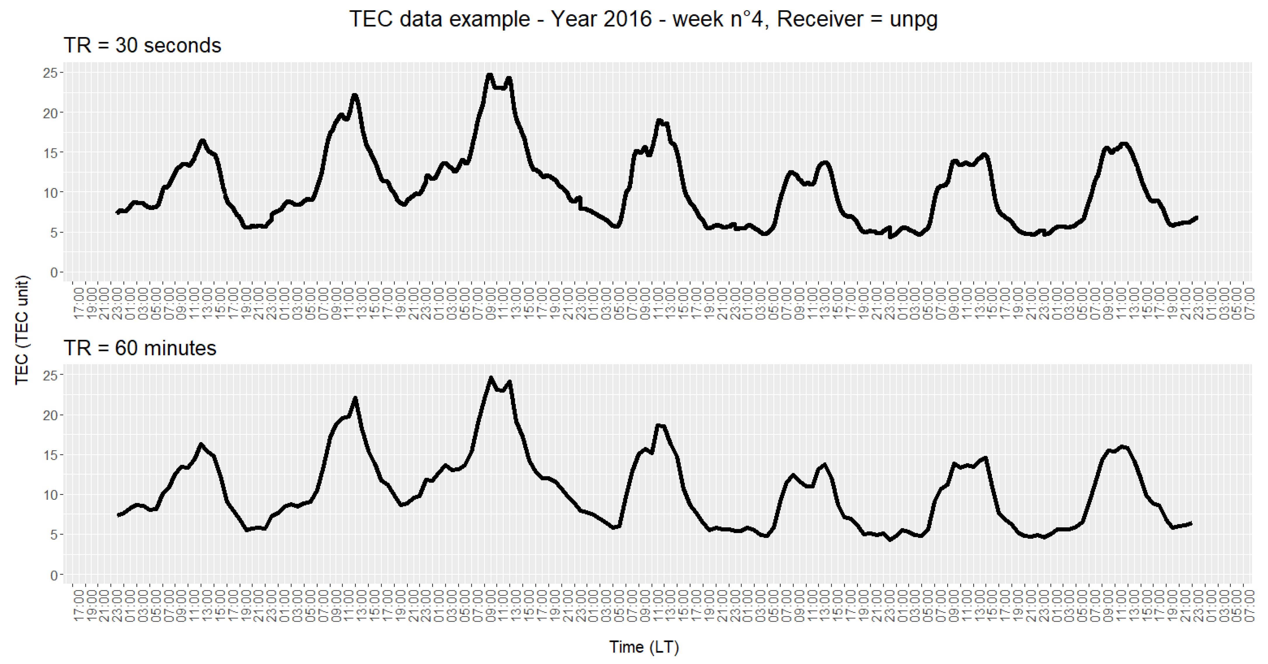
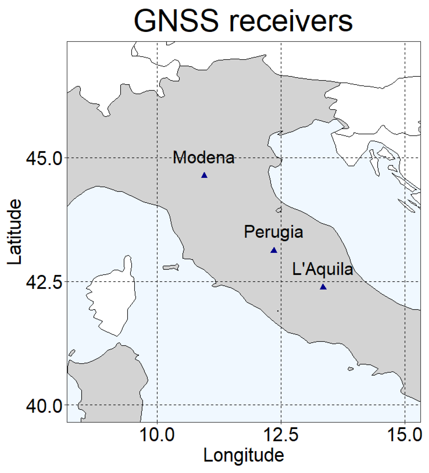
2.1. TEC Data Collection

The TEC data used in our statistical analysis are of two types:

• Single GNSS receiver data: vertical TEC (vTEC) data obtained starting from the slant TEC (sTEC) data measured by single GNSS receivers and interpolated in a point passing through the vertical of the single GNSS receiver using the IONOLAB-TEC software [28] as described in [29,30,31];
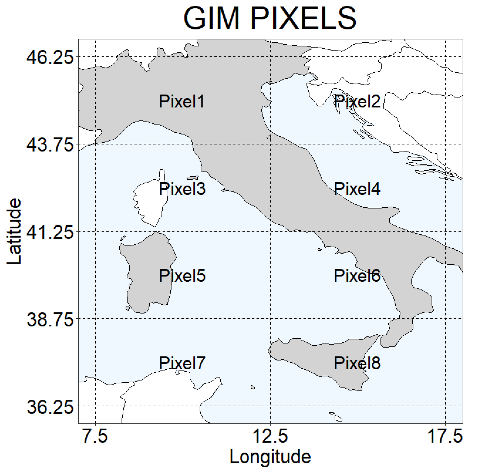
• GIM-TEC (Global Ionospheric Maps-TEC) data [32]: maps of TEC data processed and released by the Center for Orbit Determination in Europe (CODE) measured by GNSS stations and interpolated in squared areas of 2.5° of latitude and 5° of longitude (pixels) in order to cover the entire world.

If on the one hand GIM data can guarantee greater reliability in minimization of the background noise of the signal and continuity from the temporal point of view, on the other hand data obtained by single GNSS receivers can be useful to better capture any local effects of variation in the measured signal (which could have been masked by the linear interpolation over large areas practiced on the GIM data). Since there is no certainty about the size of the spatial dynamics of the phenomenon we are trying to identify, the IQR analysis was carried out on a double track, that is using both data from single stations and those from GIM maps.

Furthermore, considering that the main spatial reference for determining the earthquake preparation zone at the ground is still today (since 1979) the Dobrovolsky radius [33], which is exponentially proportional to the magnitude of the seismic event, we suppose that the effects of low-magnitude seismic events, if they occur, can be better captured by the individual receivers. Therefore, we have chosen to dedicate the data from the single stations to the study of phenomena with M ≥ 4 and the TEC-GIM data to the study of phenomena with M ≥ 5.

Regarding the time resolution (TR), the data measured by single GNSS receivers has a resolution of 30 s, while the GIM data has a resolution of 2 h. Considering the long duration required for our analysis, we preliminarily evaluated the minimum TR applicable to the GNSS data to have reasonable processing times. It was estimated to be 1 h.

The temporal resolution equal to, or greater than, 1 h is a resolution typically adopted in the literature or by international research centers that process ionospheric maps, as the temporal dynamics of the phenomenon are supposed to be relatively low. Moreover, to ensure that down sampling did not generate significant data losses, the entire study would have to be applied to both time resolutions, but this was not possible due to the long processing times that would have been necessary.

In addition, the 1-h temporal resolution also ensures homogeneity with the data of the Dst index (which also has TR = 1 h) and this protects us from the risk of attributing TEC oscillations to co-seismic activity instead due to geomagnetic activity. As an example, a comparison of one-week random TEC data with 30 s and 60 min TR is shown in Figure 2.

For the “single-stations analysis” we selected three stations of the international GNSS network on the Italian territory (whose location is shown in Figure 3 and whose coordinates are given in

Table 1. Location and data information of the aqui (L’Aquila, Italy), unpg (Perugia, Italy), mops (Modena, Italy) GNSS stations.

Station	Coordinates		Data Availability	% of Missing Data	Data Resolution
	Lat (deg)	Long (deg)	From 1 January 2001 to 31 December 2019
aqui	42.368	13.350	19 years	11.3	1 h
unpg	43.119	12.356	19 years	11.35	1 h
mops	44.629	10.949	12.8 years	9.92	1 h

), named aqui (L’Aquila, Italy), unpg (Perugia, Italy) and mops (Modena, Italy), according to the following aspects:

• Presence of seismicity around the geographical position of the GNSS receiver;
• Availability of a sufficiently long time series of data (at least 10 years);
• Minimum fraction of missing values;

Table 1 shows the main information of the 3 stations.

The TEC-GIM data used in the analysis concerned the 8 main GIM pixels covering the Italian territory between the latitudes 37.5° and 47.5° and between the longitudes 7.5° and 17.5°, as shown in Figure 4, and the time-series from 3 November 2002 to 30 June 2021.

2.2. IQR Method

Our starting point for the optimal setting of the inputs for detecting earthquake-related anomalies was the IQR method. However, the method itself has been proposed over time in several different ways by the Y.J. Liu research group (e.g., [24,25,34,35,36,37,38]) and numerous other authors (to cite some examples: [39,40,41,42]) and many improvements have been proposed. All the main input elements proposed in the various configurations will be analyzed in order to determine their convenience or otherwise in the application across Italy and the Mediterranean area. For now, we start with a basic configuration rewritten as follows in order to make it most suitable for our long-term application, according to which we have a TEC anomaly when the configuration is violated:

$$\begin{array}{c}\frac{\Delta \mathrm{TEC}}{\mathrm{MM}-\mathrm{LQ}}>\mathrm{K}\Delta \mathrm{TEC}<0\\ \frac{\Delta \mathrm{TEC}}{\mathrm{UQ}-\mathrm{MM}}\le \mathrm{K},\mathrm{if}\Delta \mathrm{TEC}\ge 0\end{array}$$

(1)

where:

–

ΔTEC is given from TEC − MM;

–

TEC is the Total Electron Content signal under investigation;

–

MM is the 15-day moving median associated to each TEC under investigation (in the same time slot and geographical location);

–

UQ and LQ are, respectively, the 15-day upper and lower quartiles associated to each TEC under investigation (in the same time slot and geographical location);

–

K is a prefixed value that acts as a threshold.

The main feature of the IQR method is the use of median and interquartile ranges associated with it (rather than mean and standard deviation) as a dynamic reference to delimit the standard behavior of the TEC. This choice, which led us to prefer IQR over other methods on which to focus our analysis, is due to the fact that the data provide a standard trend close to the lower limit. In fact, the TEC is the expression of a number of elements (electrons) and, as such, cannot assume negative values. At mid-latitudes, in the absence of external forcing (e.g., strong solar or geomagnetic activity), it generally oscillates between a few units (night) and a few tens of units (day). For this reason, the 15-day samples used as a standard reference (typically) do not have a Gaussian distribution, but a right-tailed distribution. To give an example, assuming that a measured TEC value at a certain time of day has a value of 10 TEC unit, there is a certain probability (albeit small) that one of the TEC values measured in the sample of the previous 15 days associated with it (in the same time-slot), has a value of 21 TEC unit, but there is not the same probability that an element of the 15-day sample is equal to −1 TEC unit, because this is physically impossible. This does not happen for other parameters where the lower (or upper) limit is very far from the standard behavior of the parameter (e.g., temperature measurements). From a statistical point of view, the value that best approximates to the central value of a tailed distribution is the median, and the values that best express its standard range of variation are the quartiles (see Figure 5).

Moreover, although the use of the moving median and interquartile ranges partially corrects the skewness of the TEC, a limited right-tailed asymmetry persists. This, coupled with the fact that in the IQR method the size of each value of the semi-interquartile range is not conditioned from the size of the other, led us to leave open the possibility that the positive and negative thresholds K can assume different values, respectively, Kpos and Kneg. Thus, we can rewrite Equation (1), as:

$$\mathrm{Kneg}\le \begin{array}{c}\frac{\Delta \mathrm{TEC}}{\mathrm{IQR}}\le \mathrm{Kpos}\end{array}$$

(2)

where:

–

IQR is the 15-day UQ or LQ range associated to each TEC under investigation (in the same time slot and geographical location) in a function where TEC is, respectively, greater or less than MM.

Finally, naming the term ∆TEC/IQR from the Equation (2) IQR_INDEX, we have a TEC anomaly according to Equation (3):

$$\mathrm{Kneg}\le \begin{array}{c}{\mathrm{IQR}}_{\mathrm{INDEX}}\le \mathrm{Kpos}\end{array}$$

(3)

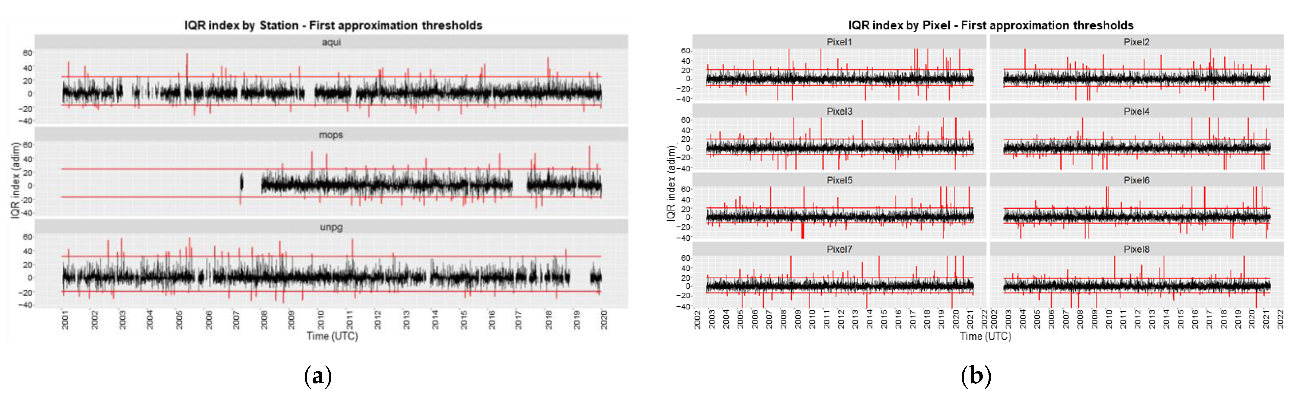
2.3. IQR_INDEX First Approximation Thresholds Setting

At this stage, we needed to determine which was the best fit for various input elements. Since starting an iterative process to find the optimal thresholds to apply to the series would have involved repeating the process at each modification made to the method, we considered it appropriate to set positive and negative (Kpos and Kneg) first approximation thresholds.

The thresholds were set sufficiently high to guarantee us the study of the most anomalous behaviors, but, given that we were going to apply other filters to the IQR_INDEX in order to try to exclude anomalies due to other natural sources (solar or geomagnetic activity), also low enough to allow us to have a statistically significant case of anomalies to analyze. We set the number of anomalies to be analyzed equal to at least 100, equally distributed by the IQR_INDEX upper and the lower values, and we took the first integer thresholds which satisfied the requirement (using a resolution of 1 TECU).

In order to do that an iterative process was performed using the R programming language to find the minimum/maximum Kpos/Kneg value for which the number of anomalies was at least 50. The obtained values are summarized in

Table 2. Minimum/maximum Kpos/Kneg values for which the number of anomalies was at least 50. The left part of the table shows the values for single GNSS stations, the right side the values of the GIM pixels method.

Station	Single Stations Thresholds		Pixel	GIM Thresholds
	Kpos	Kneg		Kpos	Kneg
aqui	24	–18	1	20	–13
unpg	31	–20	2	21	–15
mops	24	–17	3	20	–13
			4	19	–12
			5	20	–12
			6	19	–13
			7	18	–13
			8	17	–13

.

As expected, the thresholds for which 50 anomalies were detected are, in absolute value, lower for the GIM pixels and higher for the three stations. This is mainly due to the fact that GIM data, interpolated over large areas, tends to minimize local effects by flattening the signal. Furthermore, the noise level of the signal received by the individual stations is generally higher and may vary for technical reasons even from one station to another.

The thresholds also have smaller values if they refer to the negative IQR indices compared to the positive ones, confirming the previously formulated hypothesis of non-Gaussianity of the index.

In Figure 6 we show the plots of the IQR_INDEX for the TEC derived from the three Italian GNSS stations and from the 8 GIM pixels with the new threshold values (Kpos and Kneg) identified.

2.4. IQR_INDEX Inputs and Their Elements

In this section we establish which are the input variables (or just inputs) and the related input elements (which we also call just elements or input values) of the IQR method for the definition of the IQR index time-series to be used in the subsequent detection of the seismic-activity-related TEC anomalies. In particular, as input variables, we focus on the use of the persistence criterion and the management of solar conditions and of geomagnetic activity. All the input elements chosen, within each input variable, are combined with the others in order to test their validity as effectively as possible. The procedure is applied to each one of the eleven ~20-year time-series (station or pixel).

2.4.1. Persistence Criterion

The identification of seismic-related anomalies, both of ionospheric and of other natures, has often been studied in the last two decades, using the persistence criterion (e.g., [24,25,35,36,38,44]. On the basis of this criterion, it is not sufficient that a certain parameter has a behavior considered anomalous, but this behavior must also be repeated in a relatively short period of time to be classified as anomalous behavior of a seismic nature.

In order to pursue our intent to follow all the most prolific ways that in recent years have led to the detection of significant pre-seismic anomalies, we have chosen to combine the classic detection of anomalies with the detection of persistent anomalies. To identify them, we used the method implemented by Liu et al. [36] which defines Pre-Earthquakes Ionospheric Anomalous days (PEIA days) those anomalous behaviors of the parameter that are repeated for more than 1/3 of the time during a day (i.e., for 8 h out of 24).

Therefore, within the space-time interval relating to the analysis implemented in this paper, for each site (station or pixel), in the relative temporal domain and for each of the two thresholds between 0 and max/min IQR index (Kpos and Kneg), we proceeded to write lines of code able to recursively count the number of PEIA days.

As in the case of punctual anomalies, the minimum/maximum integer values for which the number of anomalies was at least 50 were extracted. These values where defined PKpos and PKneg (Persistent Kpos and Persistent Kneg). The obtained values are summarized in

Table 3. Minimum/maximum persistent Kpos/Kneg values for which the number of anomalies was at least 50. The left part of the table shows the values for single GNSS stations, the right side the values of the GIM pixels method.

Station	Single Stations Thresholds		Pixel	GIM Thresholds
	PKpos	PKneg		PKpos	PKneg
aqui	5	–5	1	4	–4
unpg	5	–4	2	4	–4
mops	5	–5	3	4	–3
			4	4	–3
			5	4	–3
			6	4	–3
			7	4	–3
			8	4	–3

.

In this case the absolute values of the thresholds are obviously lower, but also more stable and similar between the various sites. This methodology was placed side by side, without replacing it, with the classic methodology of punctual detection for comparative purposes.

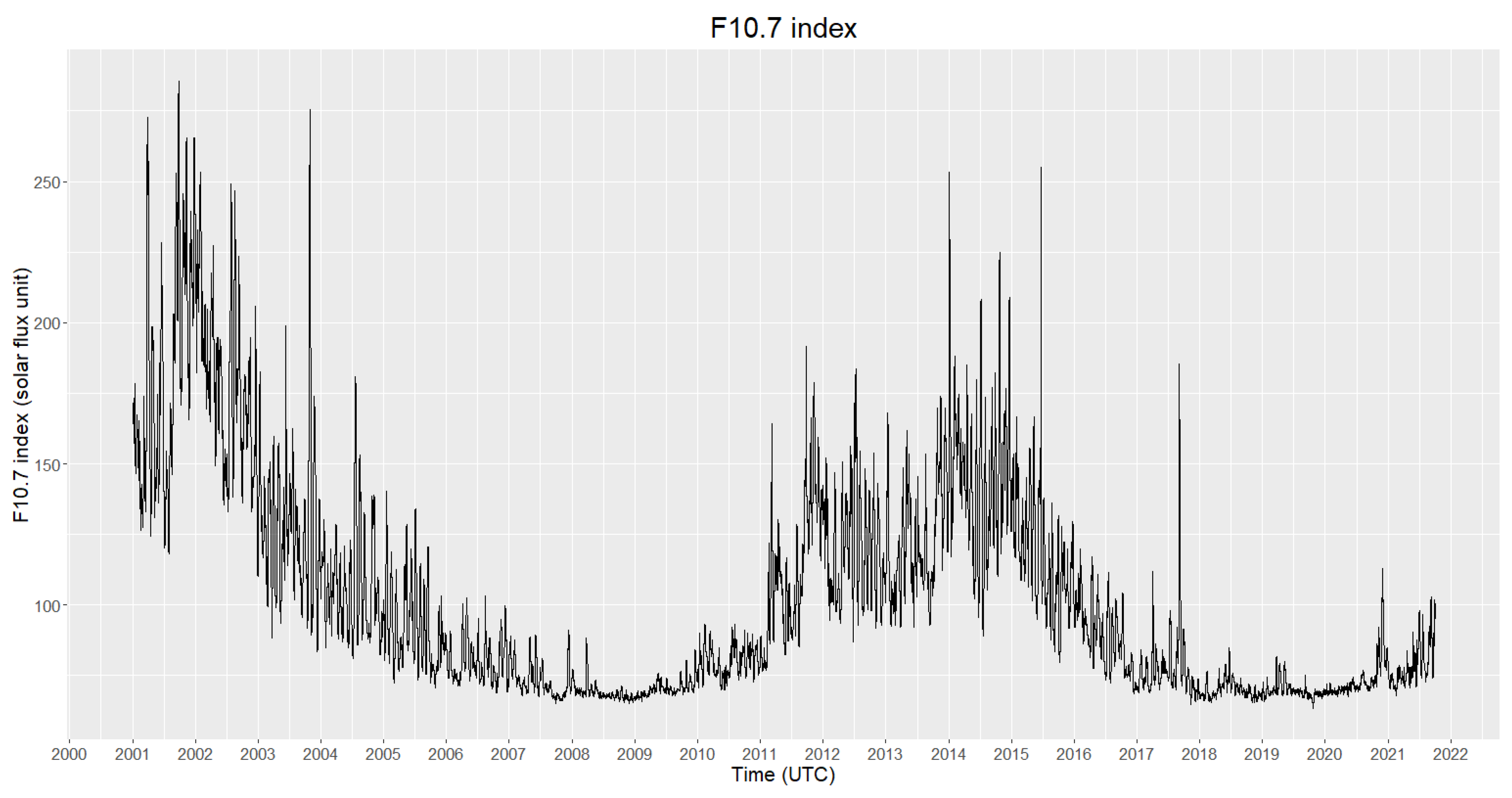
2.4.2. Management of Solar Radiation Conditions

The radiation from the Sun governs the changes in the ionospheric Total Electron Content. Over the time many authors have tried to find correlation functions between solar activity variations and TEC (e.g., [17,18,19]) but it is not easy, especially because of the strong influence of cyclic, geographical, and geomagnetic activity and other (known and unknown) source of variations.

In the IQR method, an attempt is made to evade the cyclic sources of variation (daily, 27-day, seasonal and 11-year) by building comparison samples with the data under investigation composed of a small number of daily time-slots (15 days). The starting assumption is that the variations induced by solar radiation during this period are not significant to the point of masking any anomalous behavior of the parameter connected to the seismic activity. Alongside the 15-day sliding window some authors have recently proposed the 27-day sliding window [45,46,47]. We take this evidence by introducing, in our comparisons between IQR applications, different input elements both the 15-day and alongside it the 27-day sliding window.

Furthermore, in 2009 Liu et al. [48] theorized the so-called saturation effect, i.e., the presence of a linear correlation between the daily averaged values of mean TEC and the F10.7 index, according to latitude, only as long as F10.7 does not reach the saturation threshold of about 180/200 solar flux units (sfu). Once this threshold is reached, the correlation stops being linear, but the TEC continues to vary following functions more difficult to determine and becoming more dispersed around the correlation line.

Thus, a further and more particular test carried out concerns the use of a solar activity filter, which in turn consists of a fixed threshold and a variable threshold.

In order to apply the filters, a twenty-year dataset of measured indices of solar activity F10.7 was obtained from NASA’s data supply service [49]. Using the daily measurement of the F10.7 index through a linear interpolation operation between successive values, the difference in time resolution with the TEC index (which is equal to 1 h for single receiver data and 2 h for the GIM pixels) was filled.

The twenty-year F10.7 index plotted by the R programming language is shown in Figure 7; higher variations are during solar maximum periods.

The fixed threshold is applied directly to the TEC data as a consequence of the saturation effect by using the saturation threshold of 200 sfu. Consequently, when the solar activity filter is applied the TEC data for which F10.7 is greater than 200 sfu are excluded from the analysis:

$$\mathrm{If}:\mathrm{F}10.7\ge 200\mathrm{s}.\mathrm{f}.\mathrm{u}.,\mathrm{then}:\mathrm{TEC}=\mathrm{N}.\mathrm{A}.$$

(4)

where:

–

N.A. = Not Available data.

The variable threshold for solar activity is also obtained through the application of the IQR method to F10.7 index. The purpose of this application is to ensure that sudden changes in TEC induced by sudden changes in solar activity can be recorded as such and not as potential seismic-related anomalies.

As previously stated, from a statistical point of view lower- or upper-bounded samples are typically non-Gaussian (right-tailed or left-tailed) and those that are not bounded are typically Gaussian. The measured values of the F10.7 index normally oscillate between 70 and 250 s.f.u.; the lowest value ever recorded from 1991 to date is 63.4 s.f.u. registered on 21 October 2019, and values close to 70 s.f.u. during the minimum periods of the solar cycle are very frequent (as can be seen from the graph in Figure 7). Thus, we assume that the distribution that best describes the F10.7 index behavior is (as in the case of TEC distribution) the non-Gaussian one (right-tailed). For this reason, we used the median and the related interquartile ranges (and not the mean and the standard deviation) as the central value and relative deviation that best expresses the distribution of the comparison samples with the data under investigation.

The choice of the thresholds to be used was made by relating them to the thresholds used in the IQR index applied to the TEC (Kpos and Kneg) defining a new threshold as:

$$\mathrm{Ks}=\frac{\mathrm{mean}\left(\mathrm{Kpos},\left|\mathrm{Kneg}\right|\right)}{2}$$

(5)

with:

–

Kneg and Kpos as calculated in Table 2.

Hence, the following formulas were used to calculate the F10.7_INDEX and to use it as a filter for the (TEC) IQR_INDEX.

$$\begin{array}{c}\mathrm{F}{10.7}_{\mathrm{INDEX}}=\frac{\mathrm{F}10.7-{\mathrm{MM}}_{\mathrm{F}10.7}}{{\mathrm{IQR}}_{\mathrm{F}10.7}}\end{array}$$

(6)

$$\mathrm{if}:\mathrm{F}{10.7}_{\mathrm{INDEX}}\ge \mathrm{Ks}\mathrm{or}\mathrm{F}{10.7}_{\mathrm{INDEX}}\le -\mathrm{Ks}\mathrm{then}:{\mathrm{IQR}}_{\mathrm{INDEX}}=\mathrm{N}.\mathrm{A}.$$

(7)

where:

–

F10.7 is the index value of each data point as obtained by the aforementioned interpolation having the same time resolution of the TEC under investigation.

–

MM_F10.7 is the 27-day Moving Median associated to each F10.7 under investigation (in the same time-slot).

–

IQR_F10.7 is the 27-day interquartile range associated to each F10.7 under investigation (in the same time-slot).

There is no precedent in the literature for the use of a threshold of this type for the management of the anomalies of seismic-related parameters induced by solar activity. Therefore, in this paper, we take the opportunity to introduce this new calculation tool and to test its effectiveness.

In the applications for which the IQR_INDEX must satisfy the persistence criterion to be considered anomalous, we expect that the F10.7_INDEX must also satisfy it. The related thresholds PKs are calculated as (mean (|PKneg|, PKpos))/2, taking the values obtained in Table 3. Consequently, the IQR_INDEX days for which the F10.7_INDEX threshold is exceeded for more than 8 h are excluded from the analysis.

In summary, the influence of solar radiation on the time-series of TEC data was examined by applying the changes to the IQR method presented in

Table 4. Alternative procedures tested on the IQR method for the management of solar influence.

Variations Proposed for the Management of Solar Influence
Sample size		15 days or 27 days
Solar Activity filters	Filter 1	F10.7 > 200 s.f.u. → TEC = N.A.
	Filter 2	|F10.7INDEX| > Ks → IQRINDEX = N.A.
		If in the IQRINDEX application persistence is required: F10.7INDEX > PKs for more than 8 h/day → Daily IQR index = N.A.

.

2.4.3. Management of Geomagnetic Activity

Geomagnetic activity is also an important source of TEC variation. However, within the IQR method applications (e.g., the already mentioned [24,25,38]), rather than risk losing anomalous data potentially connected to high intensity seismic events, it has often been decided to include all the ionospheric data, even those contextual to the presence of geomagnetic activity. To consider the ongoing geomagnetic activity, in these cases, a post-screening of the seismic events is sometimes carried out, while at other times, the persistence is considered to be a form of geomagnetic-filter. This last statement starts from the assumption that an anomaly recorded in a given geographical position, if persistent, is not due to geomagnetic activity measured on a global scale (see, for example, [50]). Instead, a filter on the Dst index of ±20 nT was proposed and tested in 2019, among others, by De Santis et al. [51], analyzing the electron density and magnetic field data recorded by the Swarm satellites on 1312 worldwide earthquakes of M ≥ 5.5.

Therefore, we used the data of the hourly measurements of the magnetic storm (Dst) index obtained from NASA’s data supply service [49], to apply a ±20 nT filter. In addition, in this case in order to verify the effectiveness of the filter having a term of comparison, the analyses were carried out both in the range |Dst| ≤ 20 nT and without applying the filter.

2.4.4. Recap of the IQR_INDEXES under Investigation

Table 5. Recap of the IQR index time-series under investigation according to the number of input elements with reference to the single station data recorded by aqui, unpg and mops GNSS receivers.

IQR INDEX Time-Series under Investigation—Single Station Data
Input Variable	Persistence	DSW	Sol. Filter	Geo. Filter	No. of IQR INDEXES	Station	No. of Time-Series
No. of Elements	2	2	2	2	16	3	48
Input Elements	YES	15	YES	YES		aqui, unpg and mops TEC time-series
	NO	27	NO	NO

and

Table 6. Recap of the IQR index time-series under investigation according to the number of input elements with reference to the data recorded within the 8 GIM pixels under investigation.

IQR INDEX Time-Series under Investigation—Gim Data
Input Variable	Persistence	DSW	Sol. Filter	Geo. Filter	No. of IQR INDEXES	Pixel	No. of Time-Series
No. of Elements	2	2	2	2	16	8	128
Input Elements	YES	15	YES	YES		Pixel TEC time-series from No. 1 to No. 8
	NO	27	NO	NO

offer a summary of the alternatives screened as input elements of the IQR index with reference to the 3 time-series relating to the “aqui”, “unpg” and “mops” stations and to the 8 GIM pixels covering the Italian territory in the latitude interval between 36.25° and 46.25° and in the longitude range between 7.5° and 17.5°.

Each IQR index in input can combine with the related input variables in 16 (2⁴) different ways, resulting in (48 + 128=) 176 different IQR index time-series.

2.5. Earthquake Inputs and Their Elements

Once all the potential methodological input elements that we need to test in the application of the IQR index have been defined, we must establish how these can be combined with the related seismic activity in progress. In this section we choose the earthquake input elements (concerning magnitude, space and time) of the IQR methods to be matched with the IQR indexes previously determined for the detection of the seismic-related anomalies.

In other words, we determine the earthquake magnitude-space-time (MST) domains (in which we can expect to find a correlation with the anomalous behaviors of the TEC parameter).

2.5.1. Anomaly Time Window (ATW)

We call an anomaly time window (ATW) the time around the earthquake occurrence in which we expect to find the TEC anomalies. Thus, if a TEC anomaly falls within the ATW it represents a true positive, otherwise (if it does not fall within the ATW) it is a false positive. There are no theoretical rules for determining the “earthquake preparation time”, so the ATW is basically estimated on the basis of the observations. In the early 2000s the general trend was to look for ionospheric anomalies in the 10/15 days before and after the earthquake [20,34,52,53]. However, Le et al. (2011) carried out the first of various big analyses in which seismic-related anomalies were sought in the range ±30 days around the earthquake [23]. In 2019, De Santis et al. [51] proposed and validated the ATW range of −90/+30 days.

Therefore, we chose to test the IQR index on 3 different time intervals by choosing a number of days before and after the earthquake equal to:

• ±15 days;
• ±30 days;
• −90/+30 days.

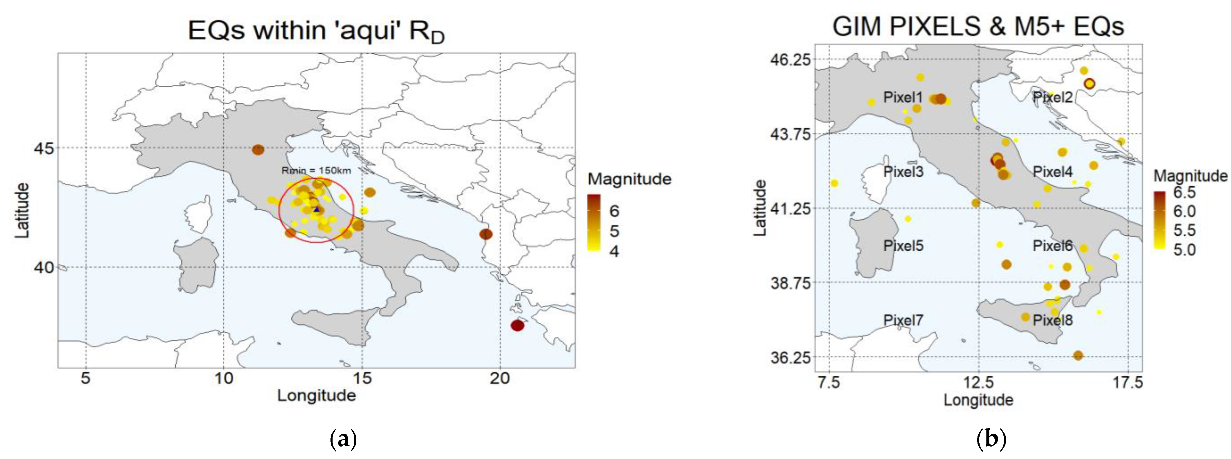
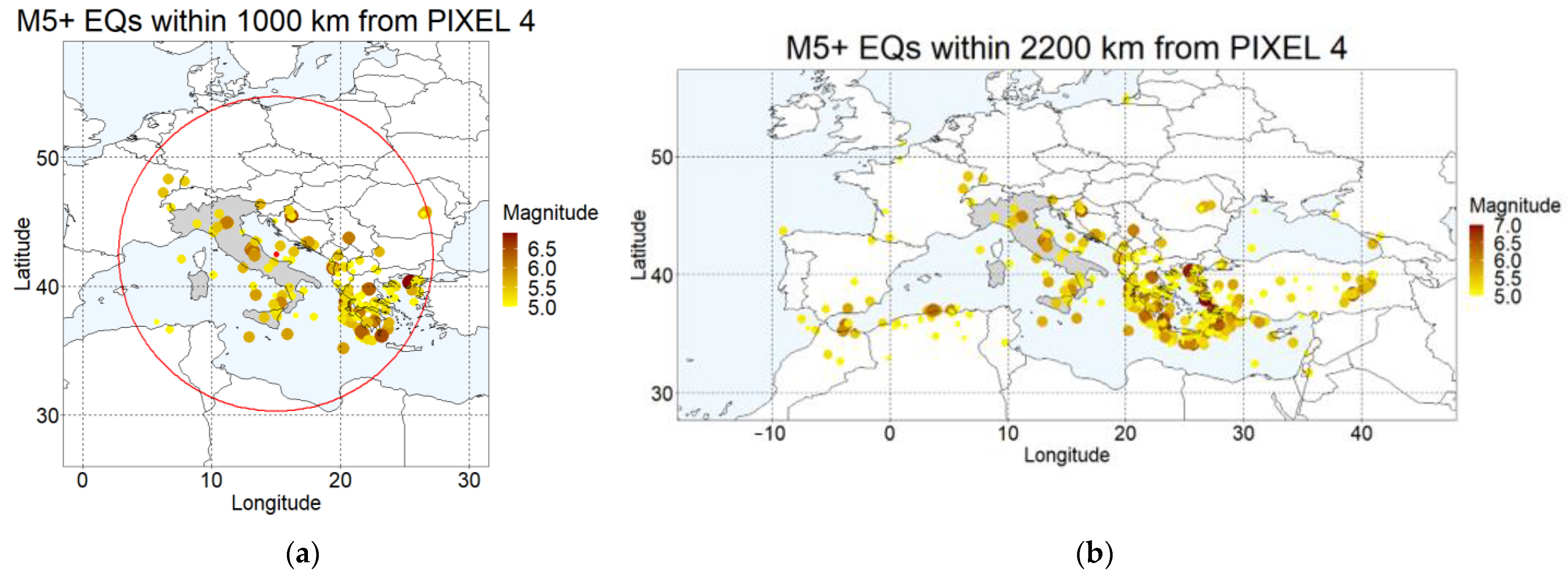
2.5.2. Space Intervals

From the spatial point of view, Dobrovolsky’s law [33] still represents the main reference for the determination of the so-called “Earthquake preparation zone”. Although it is a formula conceived and elaborated with reference to the Earth’s surface, it has also been used several times with good results in ionospheric applications (e.g., [27,46,51,54,55,56,57,58]) and other seismic-related parameters (e.g., [59,60]).

As anticipated in Section 2.1, the data coming from the single stations have the primary purpose of verifying the possible presence of local perturbations; therefore on this type of data we applied the Dobrovolsky radius with a lower limit of 150 km of radius, which is a minimum distance used by several authors over time for the detection of ionospheric anomalies (e.g., [54,56,57]) or the distance within which there are more chances to detect ionospheric anomalies according to [35].

Regarding the GIM data, looking at the criteria used by De Santis et al. [51], they found a significant number of earthquake-related ionospheric anomalies up to 1000 km from the epicenter. However, sometimes, the used “correlation distance” is also larger, e.g., C.Y. Liu et al. [38] in 2018, as part of an 18-year statistical analysis of TEC data over China, found anomalies also related to earthquakes 2070 km away from the “monitoring point” (GIM pixel used as data source). Thus, according to the distances in which ionospheric anomalies have been historically detected, we chose to check for the presence of earthquake-related anomalies in the following 3 earthquake preparation zones:

• R_D (Dobrovolsky Radius) or with the epicenter included in the Pixel Area (E_P ∈ P_A);
• R = 1000 km;
• R = 2200 km.

R is the radius calculated from the center of the GIM pixel.

Another spatial parameter to consider is the hypo-central depth. Again, according to De Santis et al. [51] earthquakes within 50 km have the highest probability of affecting the ionosphere. Therefore, as part of our analysis, we also evaluate this additional aspect using both the catalogue without depth filter (DF) and the one with the filter at 50 km.

2.5.3. Minimum Magnitude

Even with respect to the minimum magnitude at which we can assume that the ionosphere begins to feel the earthquake, the values are very variable. Generally, M5+ (e.g., [35,61,62]), M5.5+ (e.g., [51,63]) or M6+ (e.g., [23,58,64]) are used.

However, using single GNSS receivers TEC ionospheric anomalies have also been recently detected on M4+ earthquakes (e.g., [65]). The authors claim that if the station is close enough to the epicenter (in this case 13 km) local variations can be detected. Effectively, for other ground-based parameters, such as the Thermal InfreRed emission (TIR) (e.g., [66] and references within [67]), the minimum magnitude of 4 has proven to work and is normally used. In addition, the majority of the reports about significant variations of radon concentration are for M ≥ 4.0 earthquakes (as reported by [11]). It is possible that the anomalies obtained on M4+ EQs are fewer, just because they are less interesting and less investigated.

Thus, as previously stated, with the data of the individual receivers we attempted to capture the local effects (if any) of minor seismic events. Therefore, we used this type of data for M4+ earthquakes. In contrast, we considered the data deriving from the GIM maps, interpolated in very large spatial intervals (pixels with: Latitude = 2.5° and Longitude = 5°), more suitable for identifying anomalous effects related to M5+ earthquakes.

However, since, as anticipated, establishing the minimum threshold at which the ionosphere begins to feel the effects of earthquakes is still an open question, in this case we also opted for the execution of more performance tests by setting three ranges of magnitude:

• M ≥ 5;
• M ≥ 5.5;
• M ≥ 6.

2.5.4. Recap of the Earthquake Input Variables

Table 7. Recap of the MST domains and EQ catalogues under investigation according to the number of input elements with reference to the EQ data recorded around aqui, unpg and mops GNSS receivers.

MST Domains and EQ Catalogues under Investigation—Single Station Data
Input Variable	ATW	Alert Area	Max Depth	Minimum Magnitude	No. of MST Domains	Stations	No. of EQ Catalogues
No. of Elements	3	1	2	1	6	3	18
Input Elements	±15 days ±30 days −90/+30 days	D < RD or D < 150 km	NO <50 km	M ≥ 4		aqui, unpg and mops

and

Table 8. Recap of the MST domains and EQ catalogues under investigation according to the number of input elements with reference to the EQ data recorded around the 8 GIM pixels under investigation.

MST Domains and EQ Catalogues under Investigation—GIM Data
Input Variable	ATW	Alert Area	Max Depth	Minimum Magnitude	No. of MST DOMAINS	Pixels	No. of EQ Catalogues
No. of Elements	3	3	2	3	54	8	432
Input Elements	±15 days ±30 days −90/+30 days	D < RD or EP ∈ PA D = 1000 km D = 2200 km	NO <50 km	M ≥ 5 M ≥ 5.5 M ≥ 6		Pixels from No. 1 to No. 8

offer a summary of the alternatives screened as earthquake input variables and elements and a calculation of the resulting number of MST domains and earthquake catalogues with reference to the 3 GNSS stations (aqui, unpg and mops) and to the 8 GIM pixels under investigation.

The EQ input element combinations generate a potential number of 6 MST domains to be analyzed for each one of the 3 stations (18 EQ catalogues) and 54 MST domains for each one of the 8 pixels (432 EQ catalogues), for a total number of 450 EQ catalogues.

2.6. Selection of Magnitude-Space-Time (MST) Domain Case Studies

Before matching the earthquake MST domains with the combinations of the IQR index input variables, using the earthquake catalogue from the European-Mediterranean Seismological Centre (EMSC) “seismic portal project” [68], we examined the distribution of the earthquakes under investigation and the sites’ (station and pixel) locations to understand if the conditions existed to apply the proposed EQ input variables. The EMSC database contains all the European and Mediterranean earthquakes from 1st January 1998 onwards and ensures a magnitude completeness of 3 for the entire period [69].

To obtain a general idea of the seismic distribution over the selected stations and pixels in Figure 8a,b, respectively, the M4+ EQs within R_D (with R_MIN = 150 km) from one of the 3 stations examined (‘aqui’) and the M5+ EQs within the 8 GIM pixels across Italy occurring in the time domain under investigation are reported.

We started by verifying the presence of seismic events to be analyzed in the earthquake preparation areas selected for the stations and for the pixels. In

Table 9. Number of EQs occurring in the whole time and within the magnitude-space domain investigated in the framework of the analysis on the single GNSS stations.

Station	Start Date	End Date	No. of M4+ EQs with D < RD or D < 150 km
aqui	1 January 2001	31 December 2019	217
unpg	1 January 2001	31 December 2019	218
mops	5 April 2007	31 December 2019	98

the EQ numbers (occurring within the reported start/end dates, according to the TEC data availability) for each station are reported. In

Table 10. Number of EQs by minimum magnitude occurring in the whole time investigated (from 3 November 2002 to 30 June 2021) and within the pixel area or Dobrovolsky radius in the framework of the analysis on the GIM pixels.

No. of EQs with D < RD or EP ∈ PA
Min Magnitude	5	5.5	6
No. of Pixel 1 EQs	17	8	5
No. of Pixel 2 EQs	16	11	6
No. of Pixel 3 EQs	10	8	4
No. of Pixel 4 EQs	33	18	9
No. of Pixel 5 EQs	5	4	3
No. of Pixel 6 EQs	18	11	8
No. of Pixel 7 EQs	0	0	0
No. of Pixel 8 EQs	16	9	4

for each pixel the number of EQs (with D < R_D or E_P ∈ P_A) by magnitude threshold are reported.

Pixel number 7 represented the only site (station or pixel) where no earthquakes were recorded in the related MST domain, so it was excluded from the analysis.

Regarding the other 2 radii of influence proposed (R = 1000 km and R = 2200 km), the distances between the pixels were too small to avoid overlapping (the maximum distance between 2 pixels is equal to 932.6 km), so we chose to perform the proposed analyses on pixel 4, for 2 reasons: its centrality allows the analysis of the seismic events in the entire peninsula and it is the pixel within which the maximum number of seismic events occurred (see Table 10). The number of EQs within 1000 and 2200 km from the central coordinates of the Pixel 4 (from now on just R1000 and R2200 EQs) and by minimum magnitude is reported in

Table 11. Number of earthquakes by minimum magnitude within 1000 and 2200 km from the central coordinates of pixel 4 occurring from 3 November 2002 to 30 June 2021.

No. of Pixel 4 EQs	M5+	M5.5+	M6+
R1000	233	63	19
R2200	472	117	35

. The same earthquakes are shown in Figure 9.

Then, we checked the possibility of applying the depth filter (DF) to the earthquakes with a hypocenter deeper than 50 km (DF50), which would be excluded from the analysis. In

Table 12. No. of EQs under investigation (from 3 November 2002 to 30 June 2021) for each MST domain compared to the no. of these having a hypocenter deeper than 50 km.

	Site	Total	DF50	%
No. of M4+ EQs within RD/150 km for each station	aqui	217	1	0.46
	unpg	218	0	0.00
	mops	98	2	2.04
No. of M5+ EQs with D < RD or EP ∈ PA for each pixel	Pixel1	30	1	5.88
	Pixel2	33	0	0.00
	Pixel3	22	0	0.00
	Pixel4	60	1	3.03
	Pixel5	12	2	20.00
	Pixel6	37	11	38.89
	Pixel8	29	10	31.25
No. of M5+ EQs with R1000 or R2200 for Pixel 4	Pixel4	315	38	10.73
	Pixel4	624	80	11.86

the number of earthquakes and the number of DF50 earthquakes within the related space interval investigated, respectively, for each station (M4+ EQs within R_D/150 km), for each pixel (M5+ EQs within R_D/P_A) and for Pixel 4 (M5+ EQs within R1000 and R2200) are reported.

The analysis in Table 12 shows that the number of earthquakes deeper than 50 km on the Italian territory is not very relevant, except for the southeast pixels (6 and 8). Therefore, we decided to test DF on the pixels 6 and 8, which represented the MST domains in which we had statistically significant cases of DF50 EQs (on average more than 35%).

Finally, we verified the possibility of applying the three Anomaly Time Windows (ATWs) proposed in order to avoid having cumulative anomaly time windows (CATWs) so large as to occupy all (or almost all) the entire investigated time (Whole Time; WT). Since, in this sense, the temporal distribution of earthquakes (which can be grouped into seismic sequences or, on the contrary, diffuse in time) represents a fundamental element, CATW was calculated, using the R programming language, by joining (and not adding) the ATWs:

$$\mathrm{CATW}=\underset{\mathrm{i}}{{\displaystyle \cup }}{\mathrm{ATW}}_{\mathrm{i}}$$

(8)

To calculate CATW, ATW was expressed in terms of number of data points according to the temporal resolution of the TEC time-series (1 h for GNSS data and 2 h for GIM data), e.g., for the GIM data, ATW = ±30 days = 61 days = 1464 h = 732 data points. Then, for each site the anomaly time rate (ATrate) was calculated. WT is expressed in no. of data points:

$$\mathrm{ATrate}=\frac{\mathrm{CATW}}{\mathrm{WT}}$$

(9)

We decided to preliminarily exclude from the analysis the EQ catalogues for which ATrate was greater than 0.9 (90%).

Table 13. Anomaly Time rate (ATrate) for each Anomaly Time Window (ATW) and for each combination of site, R and M_MIN under investigation.

SITE	R	MMIN	ATrate (%) FOR EACH ATW (Days)
			ATW ±15	ATW ±30	ATW −90+30
AQUI	RD	4	28.6	47.3	70.7
UNPG	RD	4	29.3	45.6	67.6
MOPS	RD	4	29	49.1	73.6
PIXEL 1	RD	5	4.7	9.2	17.4
PIXEL 2	RD	5	5.1	9.9	18.1
PIXEL 3	RD	5	3.8	7.4	13.4
PIXEL 4	RD	5	9.9	19.9	35
PIXEL 5	RD	5	1.4	2.7	4.7
PIXEL 6	RD	5	6.9	13.7	26.5
PIXEL 8	RD	5	6.2	12.1	22.6
PIXEL 4	R1000	5	52.9	78.9	94.3
PIXEL 4	R2200	5	78.7	96.1	99.7
PIXEL 4	R1000	5.5 *	19.8	34.8	54.4
PIXEL 4	R2200	5.5 *	35.4	57	79.4

* M6+ is not shown because the required criteria is already verified for M5.5+.

shows the ATrates by ATW, site, R and M_MIN. From now on, the proposed area of influence for the individual stations and the minimum area of influence proposed for the pixels are simply defined R_D, knowing that in the first case we are referring to D < R_D or D < 150 km and in the second to D < R_D or E_P ∈ P_A.

Following the calculation of the ATrates shown in Table 13, the MST domains of Pixel4 R1000 with ATW −90+30 and Pixel4 R2200 with ATW −90+30 and ±30 were excluded from the analysis. To better clarify the meaning of this choice, we want to point out that for high ATrates, the results, even if they were good, would be of little practical use given the high probability of a seismic event M5+ occuring in such large space-time interval.

Recap of the Selected MST Domains and EQ Catalogues

Table 14. Recap of the selected EQ catalogues under investigation according to the number of input elements.

EQ Catalogues under Investigation
Type of Observation	MST Domains					No. of Site Catalogues	No. of EQ Catalogues
	Input Variable:	D	DF	M	ATW (Days)
Single Station data	No. Of Elements	1	1	1	3	3	9
	Input Elements	RD	NO	4+	±15; ±30; −90/+30	aqui; unpg; mops
GIM data—All pixels—Rd	No. Of Elements	1	1	3	3	7	81
	Input Elements	RD	NO	5+; 5.5+; 6+	±15; ±30; −90/+30	Pixel no. 1–6, 8
	No. Of Elements	1	1	3	3	2
	Input Elements	RD	YES	5+; 5.5+; 6+	±15; ±30; −90/+30	Pixel no. 6, 8
GIM data—Pixel no. 4—R1000/R2200	No. Of Elements	1	2	1	2	1	30
	Input Elements	R1000	Yes/No	5+	±15; ±30	Pixel no. 4
	No. Of Elements	1	2	1	1	1
	Input Elements	R2200	Yes/No	5+	±15;	Pixel no. 4
	No. Of Elements	2	2	1	3	1
	Input Elements	R1000/R2200	Yes/No	5.5+	±15; ±30; −90/+30	Pixel no. 4
	No. Of Elements	2	2	1	3	1
	Input Elements	R1000/R2200	Yes/No	6+	±15; ±30; −90/+30	Pixel no. 4
Total No. of EQ catalogues							120

and

Table 15. Recap of all the MST domains under investigation.

MST Domains under Investigation
Type of Observation	Single Station	GIM Data—Rd	GIM Data—Pixel No. 4	Total No. of MST Domains
No. of MST domains	3	18	30	51

provide a recap of the EQ input combination to be examined after the selection made in the previous section and of the resulting MST domains and EQ catalogues.

The total number of EQ catalogues to be investigated is 120, of which 9 cross with the data of the individual GNSS stations and 111 with the GIM data. The total number of MST domains under investigation is 51, 3 of which are “GNSS receiver domains” and 48 are “GIM pixel domains”.

2.7. Matching IQR and EQ Inputs

At this point, we crossed the IQR_INDEX time-series generated in Section 2.4, with the relative MST domains and EQ catalogues that we built in Section 2.5 and subsequently selected in Section 2.6 so as to determine all the possible matches. The IQR_INDEXES created were 16 (see Table 5 and Table 6) and the MST domains 51 (see Table 15), so, the total number of matches is given by the product between IQR indexes and MST domains (as in

Table 16. Total number of IQR methods under investigation.

Total No. of MST Domains	No. of IQR Indexes	Total No. of IQR Methods under Investigation
51	16	816

).

In contrast, to calculate the number of IQR time-series under investigation we had to match IQR indexes and EQ catalogues (as in

Table 17. Total number of IQR time-series under investigation.

Type of Observation	No. of IQR Indexes	No. of EQ Catalogues	No. of IQR Time-Series under Investigation
Single Station data	16	9	144
GIM data—Rd		81	1296
GIM data—Pixel no. 4		30	480
Total No. of IQR time-series under investigation			1920

).

In the following section we show how we measured the performances of the developed methods.

2.8. Positive Likelihood Ratio (LR+)

In order to test the large number of methodological alternatives proposed in the previous sections, it is fundamental to define a single measurable statistical output for each IQR method, such as a “performance index”, which allows us to classify the methodologies and their inputs and to simplify the choices between them. Using for each time-series under investigation the number of verified alarms (TPs; True Positives), False Positives (FPs) and the already defined variables Cumulative Anomaly Time Window (CATW, see Equation (8)) and Whole Time (WT, see Equation (9)), we calculated the two statistical parameters True Positive Rate (TPR) and False Positive Rate (FPR) as:

$$\mathrm{TPR}=\frac{\mathrm{TPs}}{\mathrm{CATW}};\mathrm{FPR}=\frac{\mathrm{FPs}}{\mathrm{WT}-\mathrm{CATW}};$$

(10)

and, from these, the statistical Positive Likelihood Ratio (LR+):

$$\mathrm{LR}+=\frac{\mathrm{TPR}}{\mathrm{FPR}};$$

(11)

The LR+ represents a synthetic index of a statistical type that perfectly encompasses the characteristics required for our analysis (i.e., comparison of samples of different size), as it is proportional to the number of TPs and inversely proportional to the number of FPs, both weighed on the times in which they can occur. LR+ can range from 0 (if there are 0 TPs) to infinite (if there are 0 FPs and TPs is greater than 0).

Note that, since anomalies are weighted by the time they can occur, the LR+ index is independent of the size of the Cumulative Anomaly Time Window (CATW). To give an example, suppose that during the whole time investigated we have: ATrate = 75%, TP = 3 and FP = 1, then LR+ = 1; in the same way if: ATrate = 25%, TP = 1 and FP = 3, then LR+ = 1.

Although LR+ was used in this analysis mainly for comparative purposes, the index value can also be useful as an absolute measure of the performance of individual methods. In fact, being a relationship between TPR and FPR, if it is between 0 and 1 it is indicative of a poor performance of the method, while, if greater than 1, as it grows, it returns an indication of increasingly better performance.

Therefore, a script written in R programming language was created capable of receiving all the elements (30 elements) required by each input (9 inputs), running the corresponding lines of code and to categorize the anomalies detected according to whether they fall into CATW (True Positives) or not (False Positives) and calculate TPR, FPR and LR+.

Table 18. Summary of all the inputs and input elements combined (in various ways) within the R-code created by the authors.

Input Type	Input	Elements	No. of Elements	Description (Type of Variable/Unit of Measurement)
Site	Station /Pixel	aqui, mops, unpg, Pixel1, Pixel2, Pixel3, Pixel4, Pixel5, Pixel6, Pixel8	10	Station or pixel to analyze (character)
IQR index	DSW	15, 27	2	Daily Sliding Window (no. of days)
	SF	YES, NO	2	Solar activity Filter (logic)
	GF	YES, NO	2	Geomagnetic activity Filter (logic)
	P	YES, NO	2	Persistence criterion (logic)
MST domain	ATW	30 (±15), 60 (±30), 120 (−90/+30)	3	Anomaly Time Window (no. of days)
	DF	YES, NO	2	Depth Filter (logic)
	R	Dobrovolsky, 1000, 2200	3	Max Radius (character or km)
	M	4, 5, 5.5, 6	4	Magnitude (numeric)

shows a summary of the inputs and elements of the code.

Then, in order to classify the proposed methods on the basis of the LR+ synthetic index an iterative process was carried out, i.e., to run all the 1920 IQR time-series combinations in sequence and release the related outputs in table form.

Table 19. Example showing the first 5 rows of the inputs/outputs table on the station aqui obtained using the R-code performed.

IQR—Stations—Inputs						IQR—Stations—Outputs
Site	DSW	SF	GF	P	ATW	EQs	SEQ 1	TP	TPR	FP	FPR	ATrate	LR+
aqui	27	YES	YES	NO	±30	217	35	7	0.0157	2	0.0049	0.5196	3.2357
aqui	27	YES	NO	NO	±30	217	35	6	0.0092	2	0.003	0.4954	3.0554
aqui	27	YES	YES	NO	−90/+30	217	20	8	0.0128	1	0.0043	0.7313	2.9394
aqui	27	YES	NO	NO	−90/+30	217	20	7	0.0073	1	0.0028	0.7276	2.6209
aqui	27	YES	YES	NO	±15	217	46	5	0.0179	4	0.0069	0.3242	2.6051

¹ Number of sequences of earthquakes occurring within a single ATW, which can expand in case of overlapping.

shows, as an example, the first 5 rows (best LR+) of the inputs/outputs table processed for the single station aqui (L’Aquila, Italy). In this case, the DF (Depth Filter), R (Radius) and M (min Magnitude) inputs are missing since they are not variables but they are fixed inputs (set, respectively, to: “NO”, “Dobrovolsky” and “4”).

On the basis of the LR+ index the first intermediate results were obtained (shown in Section 3.1), which allowed us to make a first selection among the best-performing methodologies and then proceed with the final results.

2.9. IQR Optimal Thresholds

As anticipated in the previous section, the last operation foreseen for the determination of the continuous long-term IQR methods applied across the Italian region that are best suited to the identification of earthquake-related anomalies was the determination of the thresholds that return the best results. These thresholds were set by exploiting an additional performance parameter, the Random Probability (RP), and by prefixing all possible upper (Kpos) and lower (Kneg) threshold combinations (as we explain in Section 2.9.1 and Section 2.9.2). Then, we performed the optimal threshold setting by creating an R program-routine for determining the outputs of the IQR method as the threshold combinations varied.

We did not exclude the hypothesis that each site may have specific thresholds depending on various factors, both of a technical nature (e.g., different signal/noise ratio between the detection stations) and of an environmental nature (as is well known, the ionosphere is a region subjected to very complex processes, some of which are still not fully understood), so we proceeded with the determination of specific thresholds site by site.

2.9.1. True Positive Random Probability (RP)

The Random Probability (RP) linked to the True Positive (TP) output represents the probability that a number X of TP at least equal to the number of TP detected has to be randomly included in the earthquake anomaly time window.

RP was calculated using the binomial distribution law. Each anomaly detected by the method can be a verified alarm (TP) or a false positive (FP). This corresponds to an experiment with only two possible outcomes that takes value 1 (success) with probability p and value 0 (failure) with probability 1−p, with 0 < p < 1. p, in our case, is the probability of (random) occurrence of a TP and is given by:

$$\mathrm{p}=\frac{\mathrm{CATW}}{\mathrm{WT}}$$

(12)

where p is equal to ATrate, see Equation (9).

Then, if X is the variable indicating the number of successes in n trials of a binomial experiment, the probability that X takes a value equal or greater than x is given by:

$$\mathrm{P}\left(\mathrm{X}\ge \mathrm{x}\right)={\displaystyle \sum }_{\mathrm{x}}^{\mathrm{n}}\left(\begin{array}{c}\mathrm{n}\\ \mathrm{x}\end{array}\right){\mathrm{p}}^{\mathrm{x}}{\left(1-\mathrm{p}\right)}^{\mathrm{n}-\mathrm{x}}$$

(13)

where (in our case):

–

x = TP number;

–

n = number of anomalies detected;

–

n − x = FP number.

The calculation was performed for each time-series in R using the pbinom function, contained in the stats package.

To make a general recap: for a given ATW (e.g., 60 days), CATW is the union of all the ATW during the entire period investigated (e.g., 2 years), ATrate is the percentage of CATW with respect to the whole time (WT) investigated (e.g., 2 years/20 years = 10%), RP is the probability that the detected true positive anomalies could randomly fall into CATW.

2.9.2. Threshold Combinations

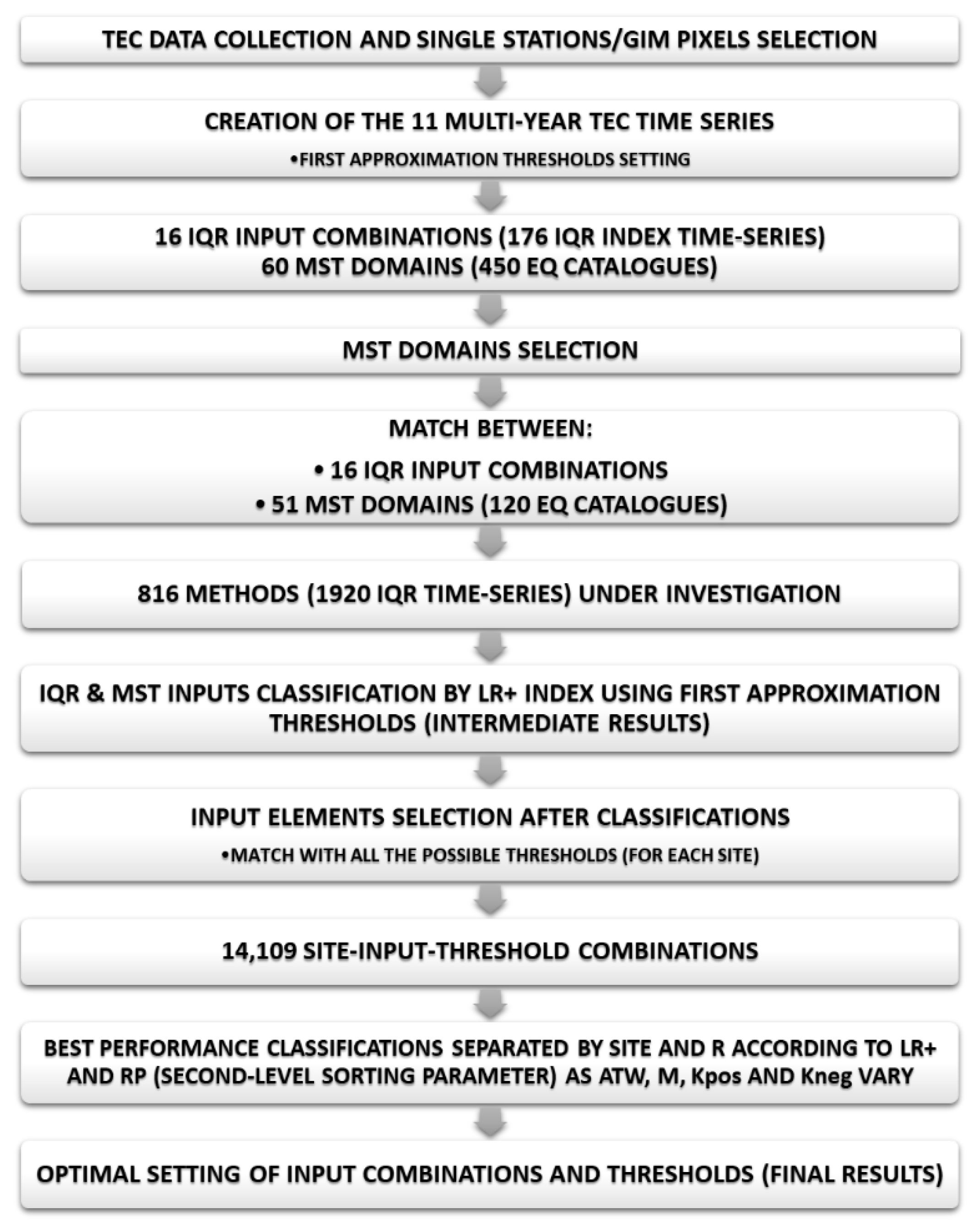
To determine all possible threshold combinations, all the limit thresholds were first calculated and then the range of variation was set. The limit thresholds were set by rounding the maximum/minimum value of each time-series to the upper/lower integer value, in order to delimit the range of variation of the data. The thresholds were varied at intervals of 2 from 3 to max IQR index value and from −3 to min IQR index value. The number of iterations performed through the threshold setting process on the IQR multi-year time series is summarized in

Table 20. Summary of the number iterations necessary for each site under investigation to achieve the optimal threshold setting.

Site	IQR Index Ranges (Rounded)		No. of Kneg Elements	No. of Kpos Elements	No. of Threshold Combinations
	Lower Limit	Upper Limit
aqui	−33	37	16	18	288
unpg	−29	45	14	22	308
mops	−29	49	14	24	336
Pixel 1	−19	47	9	23	207
Pixel 2	−19	65	9	32	288
Pixel 3	−19	33	9	16	144
Pixel 4	−19	23	9	11	99
Pixel 5	−17	27	8	13	104
Pixel 6	−15	31	7	15	105
Pixel 8	−17	29	8	14	112
Total No. of threshold combinations tested					1991

.

As a necessary step to determine the most suitable thresholds the high number of iterations resulting from the calculations shown in Table 20 was performed on each multi-year (mostly 20-year) time series using a time resolution of 1 or 2 h (according to the type of data). Despite the use of speeding-up techniques within the R programming language such a process requires long processing times. This is the main reason why in Section 3.1 we use first-approximation thresholds to set the IQR inputs in the framework of the LR+ analysis. Subsequently, in Section 3.2, we proceed to set the optimal thresholds for each of the selected best methods (input combinations). The contextual setting of the optimal thresholds would have increased the length of the process by about 100 times, furthermore the results obtained would have been difficult to manage, as conditioned by too many variables, and it would probably have been necessary to repeat the process in this phase. In this way instead, we assume that the same results are obtained, but with a faster procedure.

3. Results

As anticipated in the introductory section, typically the results from the methods proposed in the literature for the detection of earthquake-related anomalies concern the number of verified alarms, which can in turn be described according to the magnitude of the connected seismic events, the anomaly-event spatial and temporal distances, depending on whether they are pre or post seismic anomalies or according to their intensity. In rare cases the earthquake-related anomalies studies examined the occurrences of false alarms, even though the production of long-term analyses involving periods of seismic inactivity is quite rare in itself. Equally rare is the study of missed alarms, but this is a choice we share, given that, for the moment, it is quite clear that not all seismic activities produce anomalies (as pointed out by several authors, e.g., [51]), and even if this were not the case, in the current state of research on the subject we are absolutely unable to identify them all.

For the purposes we want to pursue in this paper, the study of false alarms is a fundamental element, as they also determine how much the verified alarms can be useful and how likely it is that they are actually connected to seismic activity or the result of chance.

For this reason we are less interested in the minimization of missed alarms and we are more interested in determining verified alarms (True Positives; TPs) and False Positives (FPs). However, the two values alone do not tell us much, as they also depend on the number of seismic events in the time domain or in the Anomaly Time Window (ATW) chosen: the greater the number of events or the ATW, the greater the probability that a detected anomaly falls within an ATW.

For the reasons set out above, as a first step, using the first approximation thresholds, we see with which inputs (IQR and MST) the best results in terms of LR+ are obtained, so as to get the first intermediate results, then, by setting the optimal thresholds to be applied to the previously selected methodological alternatives, we show the final results of the practical applications developed.

The steps in this section are as follows:

• IQR & MST inputs classification by LR+ index using first approximation thresholds (intermediate results);
• Selection of input elements after classification (match with all the possible thresholds);
• Determination of the best Site-Input-Threshold combinations;
• Best performance classifications separated by site and R according to LR+ and RP (second-level sorting parameter) as ATW, M, Kpos and Kneg vary;
• Optimal setting of input combinations and thresholds (final results).

It is in the steps listed above that the machine-learning process takes place, as the program automatically leverages historical data to make decisions and predictions. In summary, we can say that by analyzing the multi-year time series iteratively, the algorithm measures the performance of each single input element proposed within the multitude of possible models in order to take decisions. These decisions include the inclusion of some input elements and the exclusion of others. Then, using only the included elements and the relative residual methods, the algorithm recursively tests the multi-year time series again, contextually calculates the optimal site-input-threshold combinations and classifies them according to their performances in order to set the constraints useful to predict future anomalous behavior of the TEC parameter.

3.1. LR+ Analysis: Intermediate Results

In this section the 816 IQR methods (Table 16) and the resulting 1920 IQR time-series (Table 17) are tested, classified and selected on the basis of their input-variable performances measured by the LR+ index over the 11 sites (GNSS receivers or GIM pixels) chosen.

3.1.1. LR+ Analysis on GNSS Station Data

Starting from the GNSS stations, in

Table 21. IQR method input combinations for which the LR+ is greater than 2 in the framework of the GNSS stations analysis.

#	Site	DSW	SF	GF	P	ATW	LR+
1	aqui	27	YES	YES	NO	±30	3.24
2	aqui	27	YES	NO	NO	±30	3.06
3	aqui	27	YES	YES	NO	−90/+30	2.94
4	aqui	27	YES	NO	NO	−90/+30	2.62
5	aqui	27	YES	YES	NO	±15	2.61
6	unpg	27	YES	NO	NO	−90/+30	5.41
7	unpg	27	YES	YES	NO	−90/+30	4.97
8	unpg	27	NO	NO	NO	−90/+30	4.29
9	unpg	27	NO	YES	NO	−90/+30	2.74
10	unpg	27	YES	NO	NO	±30	2.38
11	mops	27	YES	NO	NO	±15	2.85
12	mops	27	NO	NO	NO	±15	2.84
13	mops	27	NO	YES	NO	−90/+30	2.47
14	mops	27	NO	NO	NO	±30	2.37
15	mops	27	YES	NO	NO	±30	2.36

, we show, for each station, the IQR method input combinations for which the LR+ is greater than 2. It means that a verified alarm (TP) has at least twice the probability of occurrence than a false positive (FP). We can also say that, with these input combinations, the detected anomalies are space-time connected to a M4+ EQ occurring within R_D from the reference station at least 2 times out of 3 (e.g., if the cumulative anomaly time window CATW is the 50% of the whole time WT and TP = 2 and FP = 1, then LR+ = 2). The input combinations that satisfy this requirement are 15 out of 144.

The LR+ greater than 2 are 5 for each station. All the best IQR method input combinations, require a daily sliding window of 27 days (and never 15) and never require the persistence criterion. The solar activity filter (SF) is required 10 times out of 15 and the best LR+ for each station is always registered when the solar activity filter is applied. In contrast, the filter for geomagnetic activity (GF) is required 6 times out of 15. While in the case of the aqui GNSS station, with the same other inputs, GF brings an improvement in performance, in the case of other two stations this does not happen. Finally, the effectiveness of the ATWs seems to be quite balanced, therefore it seems reasonable to think that the earthquake-related anomalies are more or less equally distributed in all 3 time intervals.

3.1.2. LR+ Analysis on GIM Data: EQs within R_D

We repeated the previous procedure over the 7 selected GIM pixels data and using R_D (or P_A) as “correlation distance”, again to find the combinations of the IQR method that return the best LR+ (greater than 2). In this case the input combinations that satisfy the requirement LR+ > 2 are 101 out of 1008 (63 EQ catalogues crossed with 16 IQR index inputs), so, to manage the high number of methodological alternatives and make a selection of the input elements valid for all the zones, we developed a classification procedure by ranks.

The procedure, developed in R, for each element of each input variable (e.g., DSW = 15 days), looks for the reciprocal (e.g., DSW = 27 days), for which the other input elements coincide. Then it classifies the pair (or triad) of values by ranks according to the highest LR+ index. The couples are ranked by 1 and 0, the triads are ranked by 3, 2, 1 (e.g., if LR+ of DSW27 is greater than LR+ of DSW15 associates 1 to DSW27 and 0 to DSW15; while if LR+ of M6+ is greater than LR+ of M5.5+ and this, in turn, is greater than LR+ of M5+ associates 3 to M6+, 2 to M5.5+ and 1 to M5+). If in the 101 combinations the routine does not find the reciprocal, it associates only 1 (3 and 2) to the element (elements) of the input present. The site is also intended as an input variable, and its value as an element; therefore, comparisons are made on the same pixel (e.g., pixel 1 is compared to pixel 1). In

Table 22. Example of scheme for determining the LR+ rank of the input variable DSW.

Input Variable	DSW	SF	GF	P	ATW	M	Site	LR+	Rank
Input elements	27	YES	YES	NO	±30	5	Pixel 1	Higher Value	1
	15							Lower Value	0

, as an example, we show the scheme of the procedure used by the program to determine a single LR+ rank for the DSW input variable.

Finally, it performs the sum of the ranks associated with each element by generating a pair (or triplet) of rank sums for each input. The rank sums results related to the 7 GIM pixels under investigation over Italy during the period 2002–2021 for the analysis performed using R_D are shown in Figure 10.

The sums of the ranks of the input combinations having LR+ greater than 2 provided further interesting indications. The 27-day DSW worked better than the 15-day DSW in 66% of the time (58 out of 88) and IQR methods worked better without applying the persistence criterion in 58% of the time (53/91), so, compared to the analysis carried out on the individual stations, the best effectiveness of the 27-day sliding windows is confirmed, as well as, albeit to a lesser extent, the best effectiveness of the methodological option in which the persistence criterion (P) is not applied.

The indications provided by the inputs ATW and M are also interesting. In this case, the data must be interpreted considering that the spatial and magnitude domains of smaller dimension are also included in those of larger dimension (e.g., the M6+ EQs are included also within the M5+ and M5.5+ domains); therefore, in general, we can assume that if the input combinations of all the variables are optimally set (LR+ > 2), the TEC seismic-related anomalies detection within R_D improves as the time of the event is approached and that the magnitude of the event increases. On the other hand, the analysis does not provide clear indications on the application of solar and geomagnetic activity filters (SF and GF).

3.1.3. LR+ Analysis on GIM Data: Depth Filter 50 km

The pixels 6 and 8 were selected to test the effectiveness of the depth filter being the pixels in which there is the greatest percentage of seismic events deeper than 50 km (see Section 2.6). Then, using the TEC data from the 2 pixels we also developed the rank sums for DF, obtaining the results shown in Figure 11.

Out of 43 pairs of methods, the methods in which the depth filter is applied work better than the others 34 times (79% of the cases). This means that in most cases (79%) the results are better if earthquakes deeper than 50 km are removed.

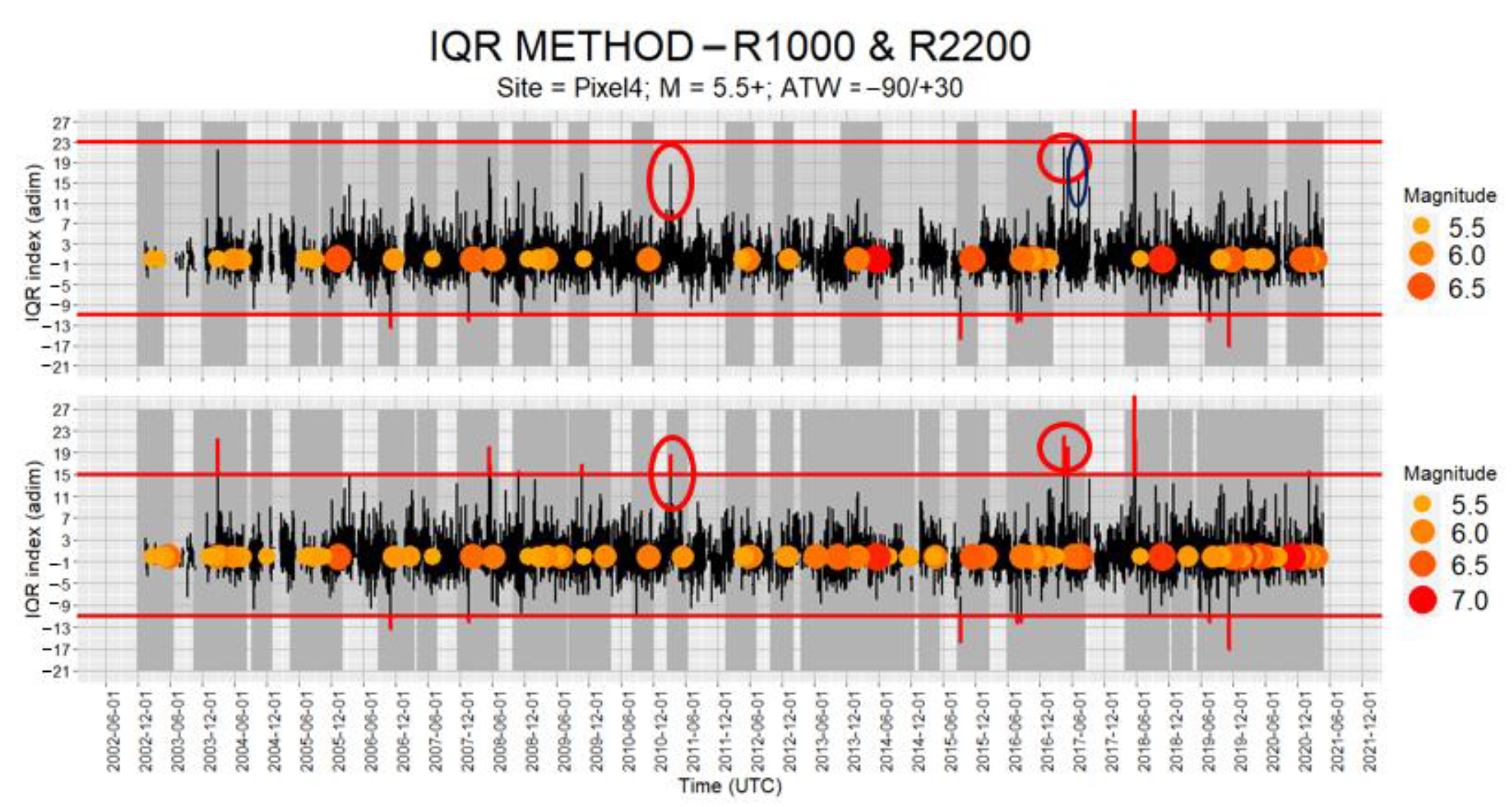
3.1.4. LR+ Analysis on GIM Data: R1000/R2200

We now examine pixel 4 (Figure 12), which is used for the analysis of larger alert areas (R1000 and R2200). As in the previous cases, we allow the inputs of the IQR index to vary, we apply the depth filter (which has been already tested) and we set R = 1000 km and R = 2200 km to check the performance of the other inputs.

Within R1000 the IQR method combinations having LR+ > 2 are 9, while within R2200 they are 13. In both cases the total number of combinations tested is equal to 144. The best effectiveness of the 27-day Daily Sliding Windows and the best effectiveness of the methodological option in which the persistence criterion is not applied, once again, are confirmed. Joining the two analyses, the 27-day DSW works better than the 15-day DSW in 92% of the time (22 out of 24) and IQR methods work best without applying the persistence criterion (P) every time.

We also obtained clearer indications regarding the application of the geomagnetic activity filter (GF). By applying GF, we achieved better performances (again by combining the two analyses) 85% of the time (22/26). In contrast, the usefulness of the solar activity filter (SF) remains uncertain. Finally, with both R1000 and R2200, the Anomaly Time Window (ATW) and minimum Magnitude (M) that worked best were the window of −90/+30 days and the magnitude 5.5+.

The M, DF and ATW input elements proposed fully confirm the input parameters proposed by De Santis et al. [51] in the analysis of electron density data. The authors, while using data from a different satellite constellation (Swarm) and using a different anomaly detection method, by examining 1312 EQs on a global scale, suggested the use of an MST domain of M5.5+, DF = 50 km and ATW = −90/+30.

3.1.5. LR+ Analysis: Results of the Input Selection

In this section we summarize the results obtained through the LR+ analysis and we choose the input elements to be used in the next section for setting the thresholds of the IQR method. We proceed by discussing the main findings for each input.

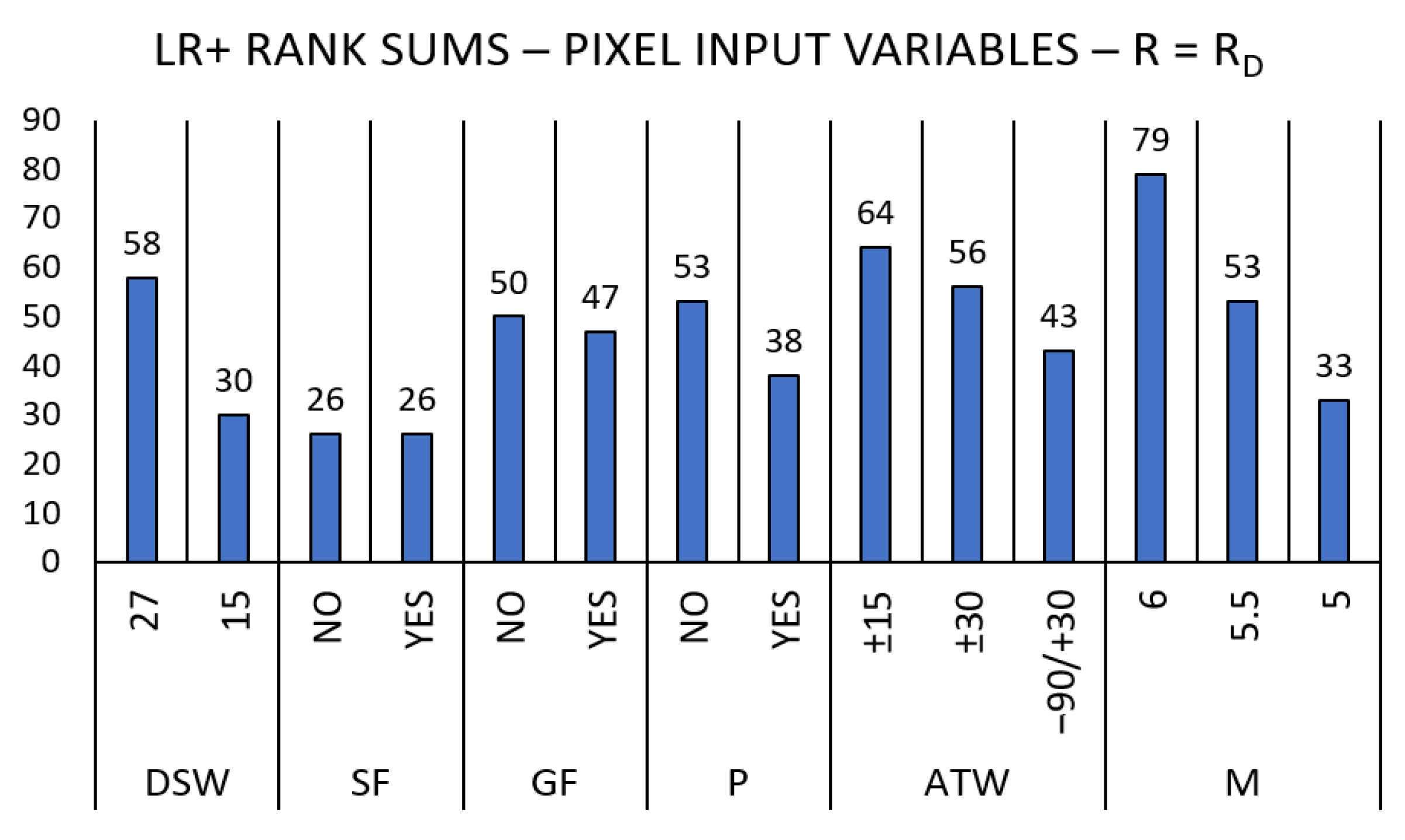
• DSW: the daily sliding window that returned the best results is undoubtedly that of 27 days. Compared to the 15-day one, it returned significantly better results both in the analysis of the individual GNSS stations and in the analyses of the GIM data.
• SF: the solar activity filter performed very well in the analysis of the single stations; the best LR+ for each station was always registered when SF was applied. The performance was neither confirmed nor denied in subsequent analyses. This is probably due to the fact that SF is related to the thresholds used for the detection of anomalies (see Section 2.3) which was higher for the individual stations than for the pixels; the lower the thresholds, the higher the IQR index values that were filtered out. Since we looked for the most anomalous behaviors of the TEC parameter, the thresholds of the GIM pixels will also rise in the next setting phase. Therefore, we decided to apply the filter for solar activity, trusting the results obtained on the individual stations.
• GF: the application of the geomagnetic activity filter gave excellent results in the analysis of the GIM data with R1000 and R2200 and uncertain results in the application on the stations as well as on the pixels with R = R_D. However, given the much greater consistency of the 2 large-area samples, we trust the GIM-data result and opted for the adoption of GF.
• P: the persistence criterion has never offered added value in any of the 3 macro analyses, so we opted for non-application.
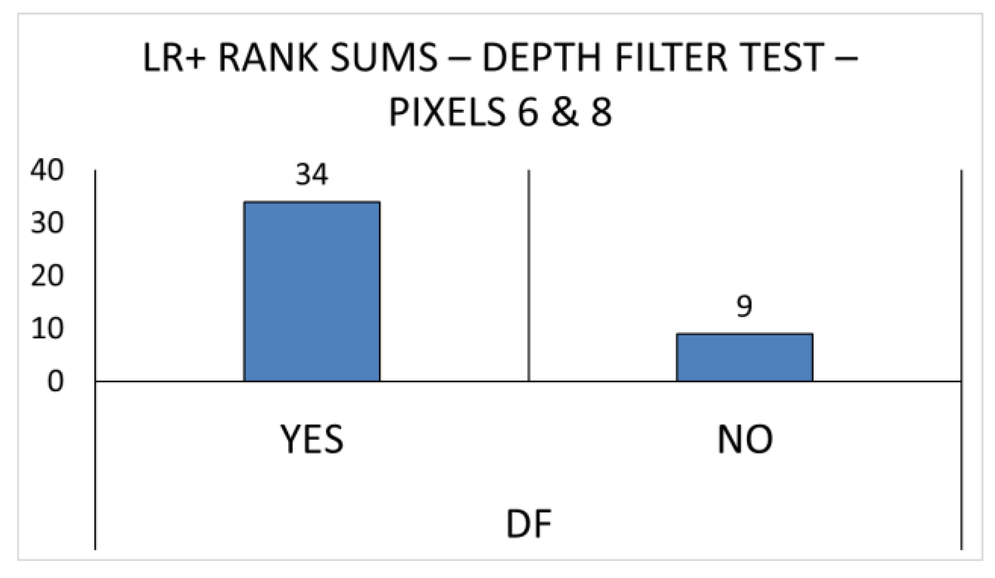
• DF: the depth filter was tested on pixels 6 and 8 (i.e., where there was a statistically significant presence of seismic events deeper than 50 km) and proved effective in 79% of cases (i.e., in 79% of cases the results are better if earthquakes deeper than 50 km are filtered out, see Section 3.1.3). Therefore, we opted to keep the filter.
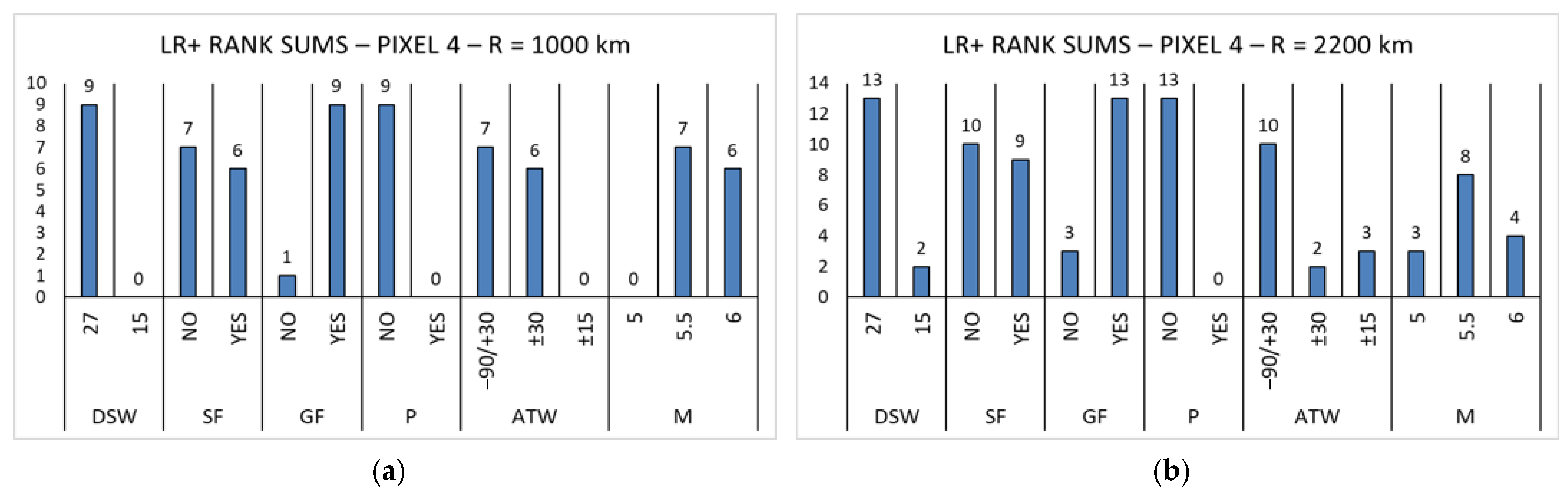
• ATW: the 3 tested anomaly time windows (±15, ±30 and −90/+30 days), in the case of the analysis across the GNSS stations having R = R_D, provided different performances according to the station under investigation; in the case of the GIM data analysis having the Dobrovolsky radius as an area of influence showed an improvement in performance as the time of the event was approached. In the case of the analysis with R = 1000 km, the ±15-day window was not effective and in the case of R = 2200 km we obtained the best performances by applying the window of −90/+30 days. Therefore, we opted to keep the 3 time windows and further verify their performance when setting the optimal thresholds and comparing the obtained results.
• M: the 3 minimum magnitudes proposed (5, 5.5, 6) in the case of R = R_D showed an improvement in performance with the increase in magnitude. In the case of the analysis with R = 1000 km and R = 2200 km, the best performance was obtained by applying M5.5+, however good performance was also obtained with R1000 and M6+. Additionally, in this case we adopted all 3 minimum magnitudes in order to test them as the thresholds changed.

Table 23. Recap of the selected input variable choices after LR+ analysis.

Type of Data	DSW	SF	GF	P	DF	ATW	M	R
GNSS Station	27	YES	YES	NO	50 km	±15, ±30, −90/+30 days	4+	RD
GIM pixel	27	YES	YES	NO	50 km	±15, ±30, −90/+30 days	5+, 5.5+, 6+	RD, 1000, 2200

shows a recap of the input variable choices after LR+ analysis to be used (further tested) in the next step (optimal threshold setting).

The IQR methods obtained by crossing the methodological inputs selected in Table 23 were in turn matched with the threshold combinations set in Table 20 in order to simultaneously determine the optimal thresholds and input combinations (see Section 3.2). The resulting combinations (applied to each site under investigation) were 14,109 (note that R1000 and R2200 were tested only on pixel 4).

Finally, the 14,109 site-input-threshold combinations under investigation were separated by Site and R and classified according to LR+ and RP (second-level sorting parameter). Since the procedure for setting the best possible thresholds in relation to the analyses performed was conducted leaving the magnitude (M) and the anomaly time window (ATW) as further variables (in addition to the thresholds Kpos and Kneg), in the following sections, we selected the cases under investigation that returned the best performance as ATW, M, Kpos and Kneg vary and then examined them, in more detail, with the help of graphs and tables.

3.2. Final Results

In this section we discuss the final results obtained. As repeatedly highlighted, we mainly focus on the minimization (zeroing if possible) of false positives, considering it useless to try to link every seismic event with anomalous behavior of the TEC parameter.

3.2.1. GNSS Stations Data IQR Method Results

The TEC data detected by the individual GNSS stations were used to investigate the presence of any local effects (D < 150 km/R_D) connected to M4+ seismic events. The analysis concerned the stations called aqui, mops and unpg, located respectively in L’Aquila, Modena and Perugia (Italy), for which the optimal thresholds were determined leaving the ATW as the only additional variable.

At the end of the iterative process, for each one of the three stations, the results obtained were filtered on the basis of the Kpos, Kneg and ATW values that returned the best LR+ index (

Table 24. Single GNSS stations IQR method outputs for which the best performance was obtained as Kpos, Kneg and ATW vary.

Kpos	Kneg	Site	ATW	EQs	SEQ	TP	FP	ATrate	LR+	RP
17	−21	aqui	±30	216	35	20	0	0.5190	Inf	0.000002
23	−23	mops	−90/+30	94	14	13	0	0.7223	Inf	0.014557
33	−19	unpg	−90/+30	217	20	10	0	0.6886	Inf	0.023969

). RP was used as a second-level sorting parameter, so that, if (as happened in this case) there were configurations for which LR+ = ∞ (FP = 0 & TP ≠ 0), they were further ordered by minimum RP.

The data obtained through the use of the individual stations yield interesting results. The number of verified alarms is relatively high overall. L’Aquila station is the one with the best output. Using the thresholds +17 and −21, 20 TP are recorded in the time interval from 30 days prior to 30 days following the seismic event. ATrate is 51.9%, which means that CATW, which is calculated only as a function of the (M4+) earthquake occurrence (considering, then, also periods for which there are no data), is approximately half of the whole time (WT). Consequently, RP, the probability that the 20 verified alarms recorded during the entire period are random, is 2 in 1 million.

In the case of the other 2 stations, the anomaly time window necessarily rises to −90/+30 days, but 13 TPs are recorded in the case of mops and 10 TPs in the case of unpg in the absence of FP. RP remain low, 1.5% for mops and 2.4% for unpg. The Kneg are overall comparable (between −19 and −23), while for the unpg station the Kpos goes up to 33 units.

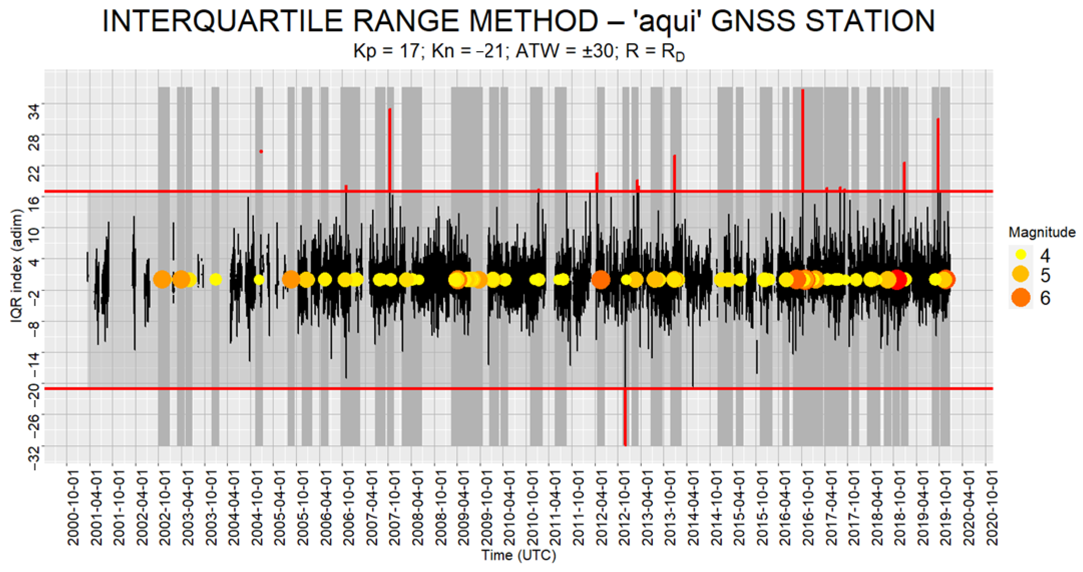
IQR Method on aqui Station

Here we see from the graphic point of view the application of the IQR method with reference to the data coming from the L’Aquila station. Figure 13 compares the IQR index trend and the M4+ earthquakes that occurred during the twenty years under investigation. In Figure 13, as well as in the following figures, all the earthquakes that occurred in the time domain are reported, including those for which the IQR index data are few or completely missing due to the solar and geomagnetic filters applied or, in the case of the GNSS stations data, for temporary tracking interruptions due to technical issues.

The graph shows a clear prevalence both in terms of the intensity and the number of anomalies towards a positive sign. It also appears that the frequency of anomalies increases with the frequency of earthquakes. Some of the 20 TPs are so close together that they are not distinguishable within the 20-year plot.

Table 25. Characterization of the TP detected by using the TEC data recorded by the GNSS station aqui (L’Aquila). Magnitudes in bold highlight (in the case of more than one seismic event alerted of by the same anomaly) the closest event in terms of time to the anomaly recorded. Dates in bold indicate earthquakes alerted of not for the first time (second or third anomaly occurrence related to the same EQ).

IQR Method—aqui Station—ATW ± 30
TP Detected				Related EQ(s)
#	IQR Index	Date	Type	M	Date	Days from TP	Dist. (km)
1	24.6	24 December 2004	POST-SEISMIC	4	9 December 2004	15	62
2	18.2	4 November 2006	POST-SEISMIC	4.5	21 October 2006	14	147
			POST-SEISMIC	4	1 November 2006	3	37
3	21.1	15 October 2007	PRE-SEISMIC	4.2	21 October 2007	−6	38
4	32.8	16 October 2007	PRE-SEISMIC	4.2	21 October 2007	−5	38
5	17.3	9 January 2011	POST-SEISMIC	4.2	9 January 2011	0	32
			PRE-SEISMIC	4	13 January 2011	−4	30
6	20.6	20 April 2012	PRE-SEISMIC	6.1	20 May 2012	−30	329
7	−31.9	28 November 2012	PRE-SEISMIC	4	5 December 2012	−7	65
8	19.2	7 March 2013	POST-SEISMIC	4.9	16 February 2013	19	76
9	18.0	15 March 2013	POST-SEISMIC	4.9	16 February 2013	27	76
10	23.9	25 December 2013	POST-SEISMIC	4.4	22 December 2013	3	131
			PRE-SEISMIC	5.2	29 December 2013	−4	144
			PRE-SEISMIC	4.4	20 January 2014	−26	144
11 12 13	17.1 36.6 25.5	9 October 2016 10 October 2016 11 October 2016	POST-SEISMIC	4.3	15 September 2016	24, 25, 26	52
			POST-SEISMIC	4.2	19 September 2016	20, 21, 22	42
			PRE-SEISMIC	4.2	16 October 2016	−7, −6, −5	43
			PRE-SEISMIC	4	26 October 2016	−17, −16, −15	53
			PRE-SEISMIC	4.7	26 October 2016	−17, −16, −15	58
			PRE-SEISMIC	4.1	26 October 2016	−17, −16, −15	60
			PRE-SEISMIC	6.1	26 October 2016	−17, −16, −15	64
			PRE-SEISMIC	4.3	26 October 2016	−17, −16, −15	59
			PRE-SEISMIC	5.5	26 October 2016	−17, −16, −15	60
			PRE-SEISMIC	4.2	27 October 2016	−18, −17, −16	56
			PRE-SEISMIC	4.4	27 October 2016	−18, −17, −16	59
			PRE-SEISMIC	4.2	27 October 2016	−18, −17, −16	71
			PRE-SEISMIC	4.4	27 October 2016	−18, −17, −16	55
			PRE-SEISMIC	4.2	27 October 2016	−18, −17, −16	70
			PRE-SEISMIC	4.4	29 October 2016	−20, −19, −18	53
			PRE-SEISMIC	4.2	30 October 2016	−21, −20, −19	50
			PRE-SEISMIC	4.6	30 October 2016	−21, −20, −19	50
			PRE-SEISMIC	4.6	30 October 2016	−21, −20, −19	57
			PRE-SEISMIC	4	30 October 2016	−21, −20, −19	58
			PRE-SEISMIC	4.1	30 October 2016	−21, −20, −19	80
			PRE-SEISMIC	4.1	30 October 2016	−21, −20, −19	53
			PRE-SEISMIC	4.6	30 October 2016	−21, −20, −19	56
			PRE-SEISMIC	4	30 October 2016	−21, −20, −19	64
			PRE-SEISMIC	4.5	30 October 2016	−21, −20, −19	43
			PRE-SEISMIC	4.2	30 October 2016	−21, −20, −19	40
			PRE-SEISMIC	4.1	30 October 2016	−21, −20, −19	49
			PRE-SEISMIC	4.1	30 October 2016	−21, −20, −19	62
			PRE-SEISMIC	4.1	30 October 2016	−21, −20, −19	44
			PRE-SEISMIC	6.5	30 October 2016	−21, −20, −19	56
			PRE-SEISMIC	4.2	31 October 2016	−22, −21, −20	53
			PRE-SEISMIC	4.3	31 October 2016	−22, −21, −20	49
			PRE-SEISMIC	4.9	1 November 2016	−23, −22, −21	72
			PRE-SEISMIC	4	2 November 2016	−24, −23, −22	61
			PRE-SEISMIC	4.8	3 November 2016	−25, −24, −23	78
			PRE-SEISMIC	4	7 November 2016	−29, −28, −27	60
14	17.7	21 April 2017	PRE-SEISMIC	4.1	27 April 2017	−6	69
			PRE-SEISMIC	4	27 April 2017	−6	71
15	17.8	05 August 2017	POST-SEISMIC	4.1	22 July 2017	14	31
16	17.4	06 September 2017	PRE-SEISMIC	4	10 September 2017	−4	31
17	22.5	28 December 2018	PRE-SEISMIC	4.3	1 January 2019	−4	57
18	17.8	28 December 2018	PRE-SEISMIC	4.3	1 January 2019	−4	57
19	18.2	29 December 2018	PRE-SEISMIC	4.3	1 January 2019	−3	57
20	30.9	21 September 2019	POST-SEISMIC	4.1	1 September 2019	20	51

shows the main information relating to the anomalies detected and the connected seismic events.

Among the 20 identified TPs, 19 were positive anomalies and 1 negative anomaly. A total of 13 anomalies were linked to single events and 7 were linked to seismic sequences. Excluding repetitions, i.e., the seismic events alerted of by more anomalies (dates of which are in bold in Table 25), the 20 TPs were connected to a total of 53 seismic events. Except for 1 earthquake, all the other 52 were within a radius of 150 km. If we consider only the (temporally) closest earthquakes in each of the 5 sequences (M in bold), on 20 TPs detected, 12 were pre-seismic and 8 post-seismic.

The 2016 sequence, consisting of 33 earthquakes that occurred between 16 October 2016 and 7 November 2016, was alerted of by 3 positive anomalies that occurred for 3 consecutive days, two of which were of high intensity, which were recorded from 7 up to 5 days before the start of the sequence. All the events of the sequence were within 80 km of the station.

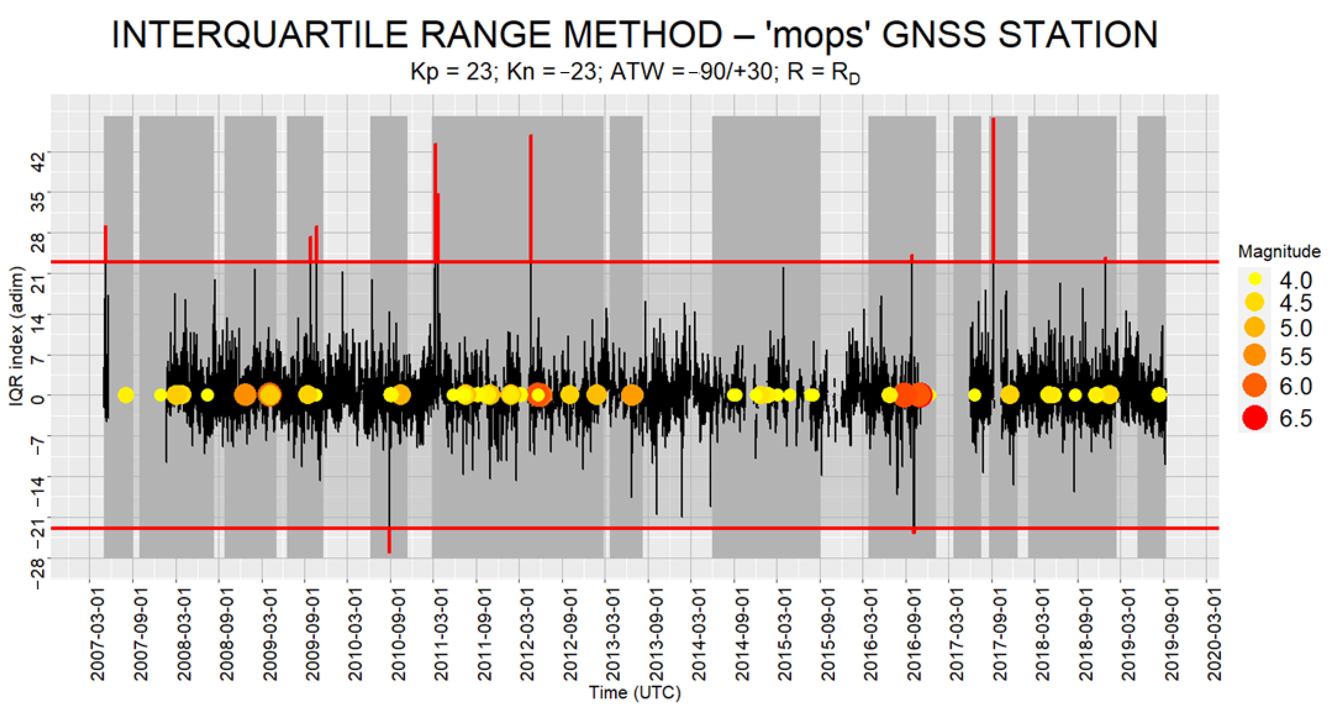
IQR Method on mops Station

In the case of the mops station 13 TPs were recorded in the absence of false positives within the ATW−90/+30 and with a random probability value equal to 0.015 (1.5%). In Figure 14 we show the related IQR method application.

Through the data coming from the mops station 13 TPs were detected. As we can see from the plot, the positive ones were more intense and more numerous (11 out of 13). In this case the 2012 seismic sequence was alerted of by a couple of pre-seismic anomalies. The details of the analysis are reported in

Table 26. Characterization of the TP detected by using the TEC data recorded by the GNSS station mops (Modena). Dates in bold indicate earthquakes alerted of not for the first time (second or third anomaly occurrence related to the same EQ).

IQR Method—mops Station—ATW−90/+30
TP Detected				Related EQ(s)
#	IQR Index	Date	Type	M	Date	Days from TP	Dist. (km)
1	29.2	7 May 2007	PRE-SEISMIC	4.2	30 July 2007	−84	76
2	27.2	27 September 2009	POST-SEISMIC	4.6	14 September 2009	13	69
			PRE-SEISMIC	4	19 October 2009	−22	91
3	29.1	22 October 2009	POST-SEISMIC	4	19 October 2009	3	91
4	–27.4	28 August 2010	PRE-SEISMIC	4.1	5 September 2010	−8	112
			PRE-SEISMIC	5	13 October 2010	−46	122
5	43.3	9 March 2011	PRE-SEISMIC	4	24 May 2011	−76	120
6	34.7	20 March 2011	PRE-SEISMIC	4	24 May 2011	−65	120
7 8	35.5 44.7	20 April 2012 21 April 2012	PRE-SEISMIC	4	19 May 2012	−29, −30	40
			PRE-SEISMIC	4	20 May 2012	−30, −31	49
			PRE-SEISMIC	4.6	20 May 2012	−30, −31	39
			PRE-SEISMIC	4.1	20 May 2012	−30, −31	44
			PRE-SEISMIC	5.2	20 May 2012	−30, −31	45
			PRE-SEISMIC	4.5	20 May 2012	−30, −31	34
			PRE-SEISMIC	4.5	20 May 2012	−30, −31	45
			PRE-SEISMIC	5.2	20 May 2012	−30, −31	34
			PRE-SEISMIC	4	20 May 2012	−30, −31	53
			PRE-SEISMIC	4	20 May 2012	−30, −31	50
			PRE-SEISMIC	4.3	20 May 2012	−30, −31	53
			PRE-SEISMIC	4.3	20 May 2012	−30, −31	41
			PRE-SEISMIC	6.1	20 May 2012	−30, −31	38
			PRE-SEISMIC	4.1	21 May 2012	−31, −32	40
			PRE-SEISMIC	4.3	23 May 2012	−33, −34	36
			PRE-SEISMIC	4	25 May 2012	−35, −36	32
			PRE-SEISMIC	4.1	27 May 2012	−37, −38	34
			PRE-SEISMIC	4.1	27 May 2012	−37, −38	36
			PRE-SEISMIC	4	29 May 2012	−39, −40	34
			PRE-SEISMIC	4	29 May 2012	−39, −40	32
			PRE-SEISMIC	5	29 May 2012	−39, −40	32
			PRE-SEISMIC	5.5	29 May 2012	−39, −40	30
			PRE-SEISMIC	4.2	29 May 2012	−39, −40	9
			PRE-SEISMIC	4.6	29 May 2012	−39, −40	29
			PRE-SEISMIC	4.2	29 May 2012	−39, −40	31
			PRE-SEISMIC	4.7	29 May 2012	−39, −40	28
			PRE-SEISMIC	4.7	29 May 2012	−39, −40	31
			PRE-SEISMIC	4.1	29 May 2012	−39, −40	34
			PRE-SEISMIC	4	29 May 2012	−39, −40	25
			PRE-SEISMIC	5.8	29 May 2012	−39, −40	31
			PRE-SEISMIC	4.2	31 May 2012	−41, −42	32
			PRE-SEISMIC	4	31 May 2012	−41, −42	31
			PRE-SEISMIC	4.9	3 June 2012	−44, −45	36
			PRE-SEISMIC	4.5	6 June 2012	−47, −48	106
			PRE-SEISMIC	4.2	12 June 2012	−53, −54	35
9	24.2	25 September 2016	PRE-SEISMIC	6.1	26 October 2016	−31, −31, −21	259
10	23.3	25 September 2016	PRE-SEISMIC	6.5	30 October 2016	−35, −35, −25	264
11	–23.7	5 October 2016	PRE-SEISMIC	4	9 December 2016	−75, −65	49
12	47.8	7 September 2017	PRE-SEISMIC	4.6	19 November 2017	−73	70
13	23.7	28 December 2018	PRE-SEISMIC	4.5	14 January 2019	−17	113

.

Except for 1 co-seismic (pre and post) and 1 post-seismic anomaly, the others were of pre-seismic type. Excluding repetitions (dates in bold), 46 earthquakes were related to the anomalies within the whole time investigated. Among the 13 TP, 5 were grouped in 1 double and 1 triple anomaly and the other 8 were single anomalies. The 2012 sequence of 35 events was alerted of by 2 intense positive anomalies (IQR index = 35.5 and 44.7) occurring less than 1 month before the first event. All the earthquakes of the seismic sequence occurred within 53 km of the station, except 1 (106 km away). As part of this sequence, the M6.1 earthquake of 20 May 2012, 38 km away from the station, was also alerted of. This event, according to Dobrovolsky’s law, was already alerted of by the GNSS station of L’Aquila which was 329 km away. The mops station also alerted of the M6.1 and M6.5 earthquakes of the 2016 sequence (which are within the Dobrovolsky radius) already alerted of by the aqui station as well. They were alerted of again by 3 anomalies, which, however, occurred on different dates (between 15 and 5 days before the aqui anomalies and between 31 and 21 days before the first main event).

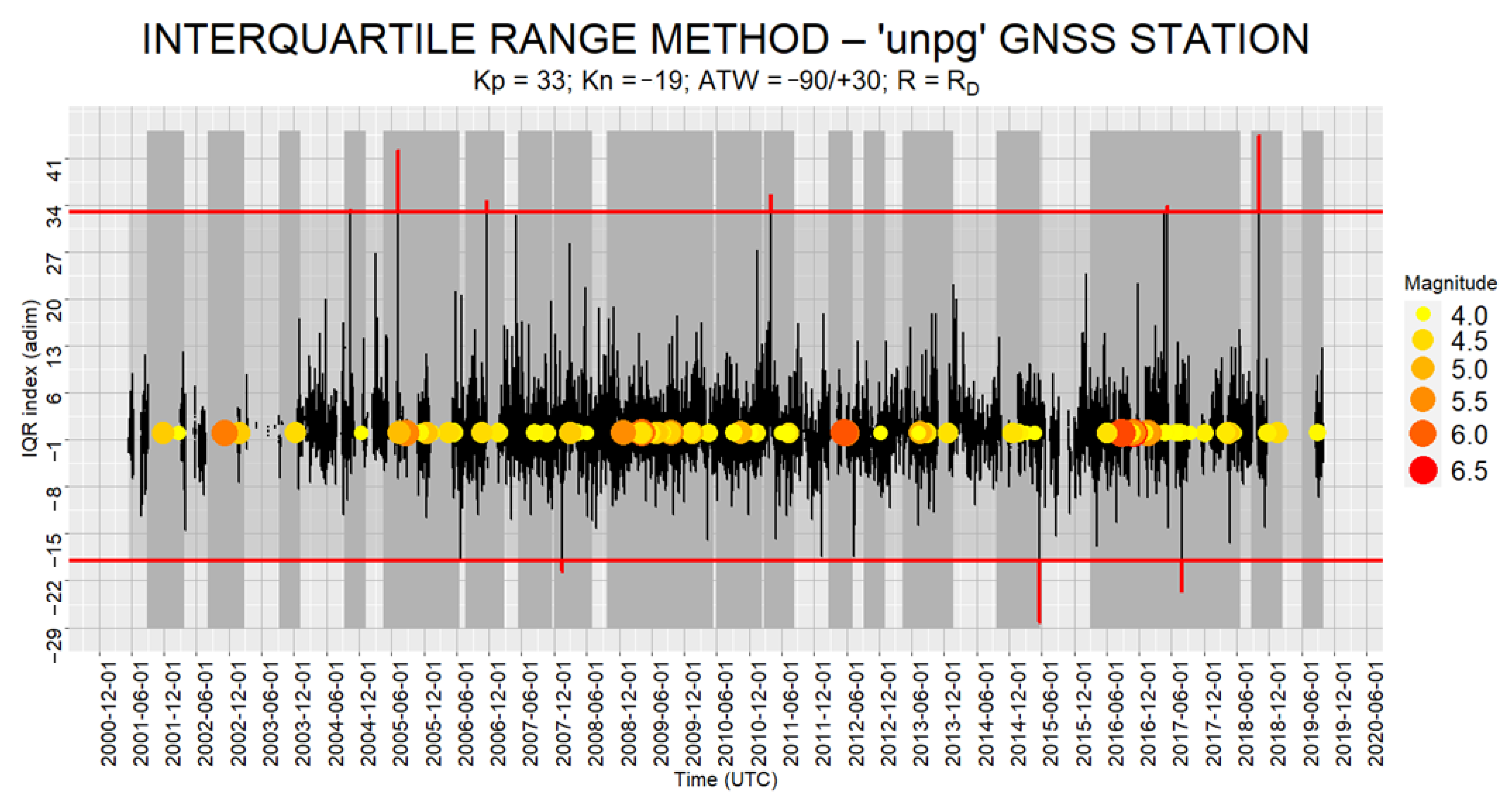
IQR Method on unpg Station

In the case of the unpg station 10 TP anomalies were recorded without FP within the ATW−90/+30 and with a random probability value equal to 0.024 (2.4%). Again, in Figure 15 we show the related IQR method application.

Through the data coming from the Perugia station 10 TP were detected, 7 of them positive while 3 were negative. The details of the analysis are reported in

Table 27. Characterization of the TP detected by using the TEC data recorded by the GNSS station unpg (Perugia). Dates in bold indicate earthquakes alerted of not for the first time (second or third anomaly occurrence related to the same EQ).

IQR Method—unpg Station—ATW−90/+30
TP Detected				Related EQ(s)
#	IQR Index	Date	Type	M	Date	Days from TP	Dist. (km)
1	33.3	9 October 2004	PRE-SEISMIC	4	9 December 2004	−61	122
2	36.2	5 July 2005	PRE-SEISMIC	4.9	15 July 2005	−10	129
3	42.2	5 July 2005	PRE-SEISMIC	5.6	22 August 2005	−48	190
4	34.7	18 November 2006	POST-SEISMIC	4.5	21 October 2006	28	79
			POST-SEISMIC	4	1 November 2006	17	80
			PRE-SEISMIC	4.3	25 January 2007	−68	109
5	−20.6	15 January 2008	PRE-SEISMIC	4.5	1 March 2008	−46	141
			PRE-SEISMIC	4.7	1 March 2008	−46	142
			PRE-SEISMIC	4.7	1 March 2008	−46	149
			PRE-SEISMIC	4.1	12 April 2008	−88	149
6	35.6	31 March 2011	PRE-SEISMIC	4	24 May 2011	−54	85
			PRE-SEISMIC	4	17 June 2011	−78	13
7	–28.2	22 May 2015	POST-SEISMIC	4	24 April 2015	28	129
8	33.8	7 May 2017	POST-SEISMIC	4.1	27 April 2017	10	60
			POST-SEISMIC	4	27 April 2017	10	58
			PRE-SEISMIC	4	20 June 2017	−44	148
			PRE-SEISMIC	4.1	24 June 2017	−48	76
			PRE-SEISMIC	4.1	30 June 2017	−54	88
			PRE-SEISMIC	4.1	22 July 2017	−76	94
9	−23.8	28 July 2017	POST-SEISMIC	4.1	30 June 2017	28	88
			POST-SEISMIC	4.1	22 July 2017	6	94
			PRE-SEISMIC	4	10 September 2017	−44	139
10	44.4	4 October 2018	PRE-SEISMIC	4.2	18 November 2018	−45	106

.

Among the 10 anomalies identified, 6 were pre-seismic, 3 co-seismic and 1 post-seismic. Excluding repetitions, the anomalies identified were linked, in the MST domain, to 21 earthquakes. Only in one case was there a double (intense) pre-seismic anomaly (2 anomalies on the same day) which occurred 10 days before an M4.9 event, followed by an M5.6 event more than a month later (the most intense of the series). The other 8 anomalies all alerted of different seismic events (or sequences of seismic events).

3.2.2. GIM Data IQR Method Results within R_D

For the GIM data application within R_D (or P_A) over the 7 pixels under investigation, at the end of the iterative process for the determination of the best IQR thresholds, the results obtained were filtered on the basis of the best LR+ values.

Table 28. IQR method outputs for the GIM-data application within R_D for which the best performance is obtained as Kpos, Kneg, ATW and M vary.

Kpos	Kneg	Site	ATW	M	EQs	TP	FP	ATrate	LR+	RP
23	−13	Pixel4	−90/+30	5	32	4	0	0.3285	Inf	0.0117
23	−17	Pixel8	±15	5	11	1	0	0.0442	Inf	0.0442
31	−13	Pixel6	−90/+30	6	7	1	0	0.0988	Inf	0.0988

shows just the best Kpos, Kneg, M and ATW combinations related to 3 pixels (among the 7 examined) for which no false positives were recorded: Pixel 4, Pixel 6 and Pixel 8.

Note that, in this case, the low number of TPs detected is probably due to the low number of M5+ events included in the relative space-time domains; in fact, in the 3 pixels a TP is detected on average every 8.3 earthquakes and the 3 pixels for which no false positives are detected are also among those with the highest number of seismic events (see

Table 29. Number of earthquakes by pixel within the Dobrovolsky radius or within the pixel area.

No. of EQs with D < RD or within PA
Pixel 4	Pixel 6	Pixel 1	Pixel 8	Pixel 2	Pixel 3	Pixel 5
33	18	17	16	16	10	5

).

The only pixel in which more than one anomaly occurred in the absence of false positives was pixel 4, i.e., the pixel with the greatest number of seismic events. The Kpos and Kneg thresholds that provided the best results varied, respectively, between 23 and 31 and between −13 and −17. The anomaly detected in pixel 6 is associated with a seismic event of M6+, while the anomaly detected in pixel 8 occurred within ±15 days of an M5+ event. The probabilities that TPs were randomly detected (RP) are all less than 0.1 (10%).

In pixel 4 the 32 EQs are grouped in 15 seismic sequences. The particularly low RP of the pixel (about 1%), combined with the TP percentage (26.7%) per number of sequences leads us to think that the technique can offer appreciable results in particularly seismically active areas.

Table 30. Characterization of the TP detected by the IQR method analysis carried out using the GIM-TEC data recorded within pixel 4.

IQR Method—PIXEL 4—M5+—ATW−90/+30—RD
TP Detected				Related EQ(s)
#	IQR Index	Date	Type	M	Date	Days from TP	Dist. (km)
1	−13.3	3 November 2006	PRE-SEISMIC	5.1	10 December 2006	−37	108
2	−16	8 September 2015	PRE-SEISMIC	6.5	17 November 2015	−70	614
3	Inf	23 May 2018	PRE-SEISMIC	5.3	16 August 2018	−85	69
4	−17	8 November 2019	PRE-SEISMIC	6.4	26 November 2019	−18	391

shows the main information from the analysis of pixel 4.

There were 3 negative and 1 positive anomalies connected to as many seismic events. All 4 identified anomalies were pre-seismic and were linked in a one-to-one way to seismic events. The magnitudes varied between 5.1 and 6.5 and the verified alarms occurred between 18 and 85 days before the events. The distances (intended from the center of the pixel) were all in the Dobrovolsky radius, but the events of M5.1 and M5.3 also fell within the pixel area.

3.2.3. GIM Data IQR Method Results within R1000

Here we see the results obtained from the analysis within a radius of 1000 km carried out using the data obtained from pixel 4. As in the previous cases,

Table 31. IQR method outputs for which the best performance was obtained in the framework of the Pixel 4 GIM-data application within R1000.

Kpos	Kneg	ATW	M	EQs	TP	FP	ATrate	LR+	RP
23	−11	−90/+30	5.5	52	9	0	0.5191	Inf	0.0027

shows the output combination which returns the best performance.

In this case the best possible combination was recorded within an anomaly window of 120 days with a minimum magnitude of 5.5 and detecting 9 TPs. The Anomaly Time is about half the total time (51.9%). The probability that the 9 anomalies were random (stochastic) results is very low (0.27%). The percentage of anomalies verified with respect to the number of earthquakes is significant 17.3% (47.4% in relation to the number of seismic sequences). Regarding the thresholds, the upper one (Kpos) was confirmed with respect to the observation within the Dobrovolsky radius, while the lower one (Kneg) dropped by 2 units, from −13 to −11 (compare with Table 28, row 1).

In Figure 16 we show, for the best input combination related to the analysis carried out on pixel 4 within the radius of 1000 km, the IQR index plot and the earthquakes occurring in the relative MST domain under investigation.

Within the radius of 1000 km from Pixel 4 the best possible combination identified 9 TP anomalies out of 52 EQs in the magnitude range M5.5+ and in the anomaly time window range −90/+30 days from the earthquake. Among the 9 anomalies detected, 8 were negative and 1 was positive.

Table 32. Characterization of the TP detected using the GIM-TEC data recorded within pixel 4 and within a distance of 1000 km from the center of the pixel. Magnitudes in bold highlight the closest event in terms of time to the anomaly detected.

IQR Method—Pixel 4—M5.5+—ATW−90/+30—R1000
TP Detected				Related EQ(s)
#	IQR Index	Date	Type	M	Date	Days from TP	Dist. (km)
1	−13.3	3 November 2006	PRE-SEISMIC	5.7	23 November 2006	−20	741
			PRE-SEISMIC	5.8	24 November 2006	−21	693
2	−12.0	22 January 2008	PRE-SEISMIC	6.3	14 February 2008	−23	876
			PRE-SEISMIC	6	14 February 2008	−23	901
			PRE-SEISMIC	5.8	20 February 2008	−29	898
3	−16.0	8 September 2015	PRE-SEISMIC	6.5	17 November 2015	−70	614
4	−11.7	24 July 2016	PRE-SEISMIC	6.2	24 August 2016	−31	148
			PRE-SEISMIC	5.5	24 August 2016	−31	155
5	−12.2	27 July 2016	PRE-SEISMIC	6.2	24 August 2016	−28	148
			PRE-SEISMIC	5.5	24 August 2016	−28	155
6	−12.1	16 August 2016	PRE-SEISMIC	6.2	24 August 2016	−8	148
			PRE-SEISMIC	5.5	24 August 2016	−8	155
			PRE-SEISMIC	5.5	26 October 2016	−71	159
			PRE-SEISMIC	6.1	26 October 2016	−71	160
			PRE-SEISMIC	6.5	30 October 2016	−75	159
7	Inf	23 May 2018	PRE-SEISMIC	5.5	25 June 2018	−33	843
8	−12.0	22 July 2019	PRE-SEISMIC	5.6	21 September 2019	−61	390
9	−17.0	8 November 2019	PRE-SEISMIC	6.4	26 November 2019	−18	391

summarizes the main correlation information between the identified TP and connected seismic events.

The first thing we notice examining the table is that all the anomalies are pre-seismic. The 9 TPs (8 were negative and 1 was positive) were fairly distributed over time, with the exception of the 3 in 2016, which occurred over 23 days and alerted of (3 times) the 2 seismic events that occurred in August 2016 of M6.2 and M5.5 (Central Italy). The 3 anomalies, although not characterized by strong intensity (they exceeded Kneg by 0.7, 1.2 and 1.1) were repeated at 31, 28 and 8 days before the two seismic events, which were located within the pixel area.

Overall, excluding repetitions, i.e., earthquake alerts occurring more than once, the 9 anomalies alerted of 13 seismic events M5.5+ out of 52 (25%), if we take only the first earthquakes in each of the 9 sequences (M in bold) and we exclude repetitions, we were alerted of 7 out of 52 events, with an anomaly time rate of 13.5%. A total of 4 of the 7 earthquakes were of M6+ and the 2 of greater magnitude (6.4 and 6.5) were also those that recorded the highest negative anomalies (−16 and −17).

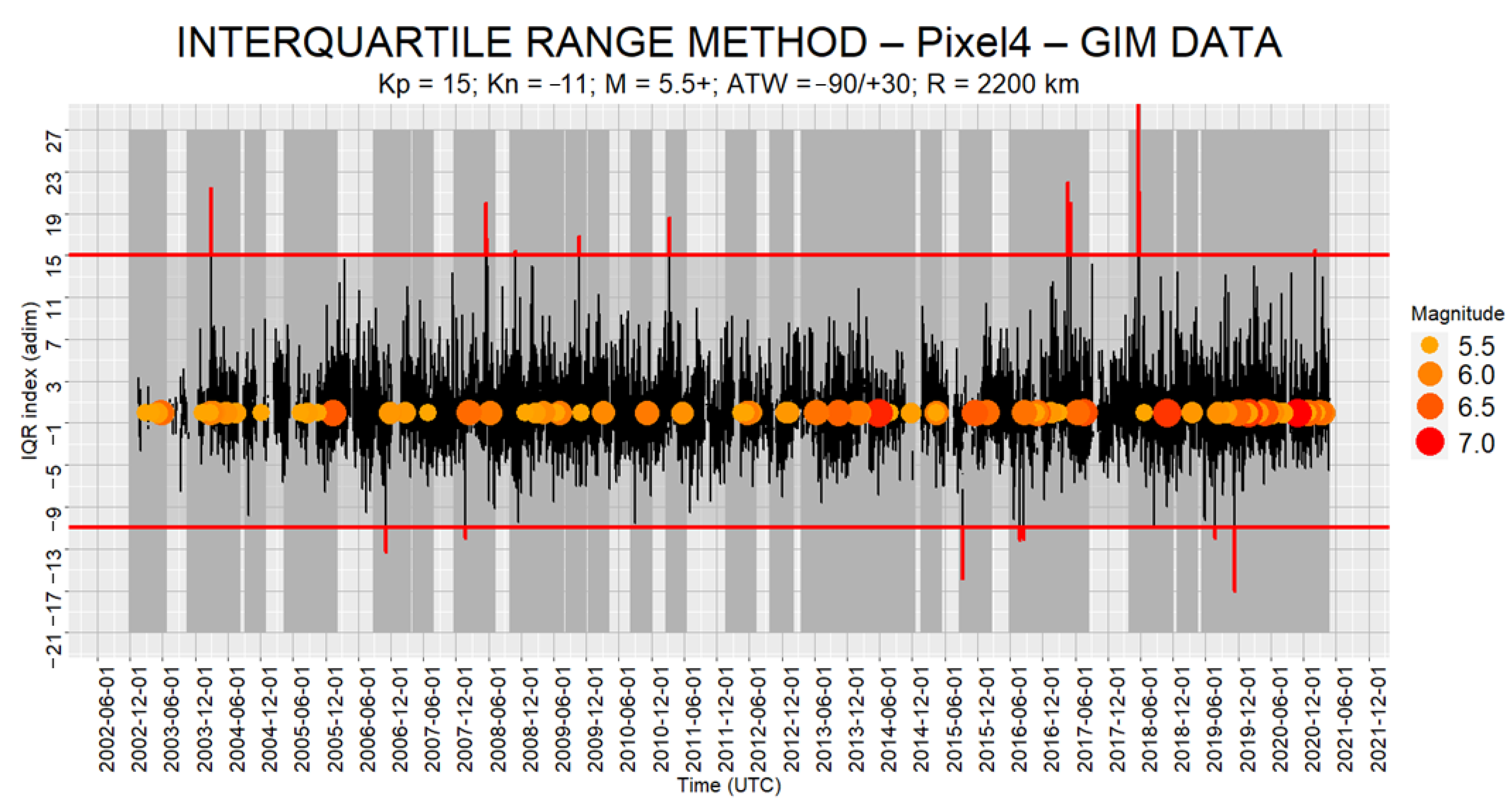
3.2.4. GIM Data IQR Method Results within R2200

In

Table 33. IQR method outputs for which the best performance was obtained in the framework of the Pixel 4 GIM-data application within R2200.

Kpos	Kneg	ATW	M	EQs	TP	FP	ATrate	LR+	RP
15	−11	−90/+30	5.5	96	22	0	0.7593	Inf	0.0023

we show the best combination results obtained from the analysis within a radius of 2200 km.

The best combination was once again recorded in the 120-day time window with M5.5+. The verified alarms totaled 22. The ATrate is higher compared to the R1000 analysis (75.9% vs. 51.9%), but the random probability is even lower (0.23% vs. 0.27%). The Kneg threshold remains unchanged, while the Kpos threshold is lowered by 8 units, from 23 to 15.

In Figure 17 we show, for the best input combination related to the analysis carried out on pixel 4 within the radius of 2200 km, the IQR index plot combined with the earthquakes occurring in the relative MST domain under investigation.

Within the radius of 2200 km from Pixel 4 the best possible combination identified 22 TP anomalies out of 96 EQs in the magnitude range M5.5+ and in the anomaly time window range −90/+30 days from the earthquake. Among the 22 anomalies detected, 8 were negative and 14 were positive.

Table 34. Characterization of the TP detected using the GIM-TEC data recorded within pixel 4 and within a distance of 2200 km from the center of the pixel. Magnitudes in bold highlight the closest event in terms of time to the anomaly detected. EQ dates in bold indicate earthquakes alerted of not for the first time (second or third anomaly occurrence related to the same EQ). TP dates in bold indicate the anomalies identified following the extension of the radius from 1000 to 2200 km (cfr. Table 32).

IQR Method—Pixel 4—M5.5+—ATW−90/+30—R2200
TP Detected				Related EQ(s)
#	IQR Index	Date	Type	M	Date	Days from TP	Dist. (km)
1	21.5	28 February 2004	POST-SEISMIC	5.5	23 February 2004	5	874
			POST-SEISMIC	6	24 February 2004	4	1829
			PRE-SEISMIC	5.5	1 March 2004	−2	848
			PRE-SEISMIC	5.9	17 March 2004	−18	1128
			PRE-SEISMIC	5.8	23 May 2004	−85	228
2	−13.3	3 November 2006	PRE-SEISMIC	5.7	23 November 2006	−20	741
			PRE-SEISMIC	5.8	24 November 2006	−21	693
3	21.0	7 May 2007	PRE-SEISMIC	5.5	29 June 2007	−53	573
4	−12.0	22 January 2008	PRE-SEISMIC	6.3	14 February 2008	−23	876
			PRE-SEISMIC	6	14 February 2008	−23	901
			PRE-SEISMIC	5.8	20 February 2008	−29	898
5	20.0	19 May 2008	PRE-SEISMIC	6.1	8 June 2008	−20	745
6	16.6	20 May 2008	PRE-SEISMIC	6.1	8 June 2008	−19	745
7	15.4	30 October 2008	PRE-SEISMIC	5.5	23 December 2008	−54	436
8	16.8	22 October 2009	PRE-SEISMIC	5.5	3 November 2009	−12	725
9	15.6	22 October 2009	PRE-SEISMIC	5.5	3 November 2009	−12	725
10	18.6	9 March 2011	PRE-SEISMIC	5.8	19 May 2011	−71	1247
11	−16.0	8 September 2015	PRE-SEISMIC	6.5	17 November 2015	−70	614
12	−11.7	24 July 2016	PRE-SEISMIC	6.2	24 August 2016	−31	148
			PRE-SEISMIC	5.5	24 August 2016	−31	155
13	−12.2	27 July 2016	PRE-SEISMIC	6.2	24 August 2016	−28	148
			PRE-SEISMIC	5.5	24 August 2016	−28	155
14	−12.1	16 August 2016	PRE-SEISMIC	6.2	24 August 2016	−8	148
			PRE-SEISMIC	5.5	24 August 2016	−8	155
			PRE-SEISMIC	5.5	26 October 2016	−71	159
			PRE-SEISMIC	6.1	26 October 2016	−71	160
			PRE-SEISMIC	6.5	30 October 2016	−75	159
15	22.0	20 April 2017	PRE-SEISMIC	6.3	12 June 2017	−53	1037
16	20.0	8 May 2017	PRE-SEISMIC	6.3	12 June 2017	−35	1037
			PRE-SEISMIC	6.6	20 July 2017	−73	1230
17	Inf	23 May 2018	PRE-SEISMIC	5.5	25 June 2018	−33	843
18	16.0	25 May 2018	PRE-SEISMIC	5.5	25 June 2018	−31	843
19	21.0	26 May 2018	PRE-SEISMIC	5.5	25 June 2018	−30	843
20	−12.0	22 July 2019	PRE-SEISMIC	5.8	8 August 2019	−17	1344
			PRE-SEISMIC	5.6	21 September 2019	−61	390
			PRE-SEISMIC	5.7	26 September 2019	−66	1112
21	−17.0	8 November 2019	PRE-SEISMIC	6.4	26 November 2019	−18	391
			PRE-SEISMIC	5.6	22 January 2020	−75	1148
			PRE-SEISMIC	6.8	24 January 2020	−77	2098
			PRE-SEISMIC	5.7	30 January 2020	−83	1381
			PRE-SEISMIC	5.6	30 January 2020	−83	1388
22	15.5	2 February 2021	PRE-SEISMIC	5.5	17 February 2021	−15	747
			PRE-SEISMIC	6.3	3 March 2021	−29	677
			PRE-SEISMIC	5.8	4 March 2021	−30	669
			PRE-SEISMIC	5.6	12 March 2021	−38	658
			PRE-SEISMIC	6	18 March 2021	−44	1042
			PRE-SEISMIC	5.5	27 March 2021	−53	114

shows the main information from the analysis.

In addition, in this case the 22 verified anomalies were mainly of a pre-seismic type except for no. 1, which was co-seismic (pre- and post-seismic). Using the MST domain M5.5+, R2200 and ATW−90/+30, 47 seismic events were connected to the 22 TPs. A total of 29 of them had magnitudes between 5.5 and 5.9, while 18 of them were M6+ events. The earthquake-anomaly temporal distances varied between −85 and +5 days and the spatial distances between 114 and 2098 km. If we select only the 22 earthquakes closest to the 22 detected seismic-related anomalies (whose magnitudes are in bold) and we exclude the seismic events connected to more than one anomaly (whose dates are in bold), the 22 TPs alerted of in total 15 seismic events (3 of which are alerted of by 2 TPs and 2 of which are alerted of by 3 TPs).

Compared to the R1000 case (in which 9 TPs were detected), only the radius of influence varies (the other inputs are identical). The extension of the radius up to 2200 km generates the detection of 13 other TPs. The TP dates in bold identify these 13 TPs. All 13 were positive anomalies; in fact, the lower threshold has remained unchanged (−13) while the upper one has dropped by 8 units (from 23 to 15). This gave us the opportunity to compare the two radii of influence (R1000 and R2200), whose IQR indices in relation to seismic activity are shown again together in Figure 18.

The vertical grey ribbons that delimit the ATWs in the IQR method plots help to understand if the corresponding IQR index falls in an alert time window or not. Comparing the plots in Figure 18 we note that the lowering of the Kpos threshold from the R1000 case to the R2200 case is due to the transformation of the IQR index values 18.6 and 22 of 9 March 2011 and 20 April 2017 (red circles in Figure 18 and TP no. 10 and 15 in Table 34) from FP (in the case of R1000) to TP (in the case of R2200).

The distances from the pixel center of the 2 connected seismic events (distances in bold in Table 34), do not exceed 1250 km and by scrolling down the column relating to the distances we can see that within this radius of influence all 22 TPs would still be confirmed.

Therefore, by increasing the radius R1000 to 1250 km, there would be a lowering of the upper threshold of up to 15 which would generate the same number of TPs (22) that are recorded in the R2200 case, but in a considerably reduced area. The only value that would be higher than the threshold Kpos = 15 would be the one circled in blue, which, however, is connected to a variation of solar activity (whose filter is linked to the thresholds); for this reason in the R2200 graph it is no longer present.

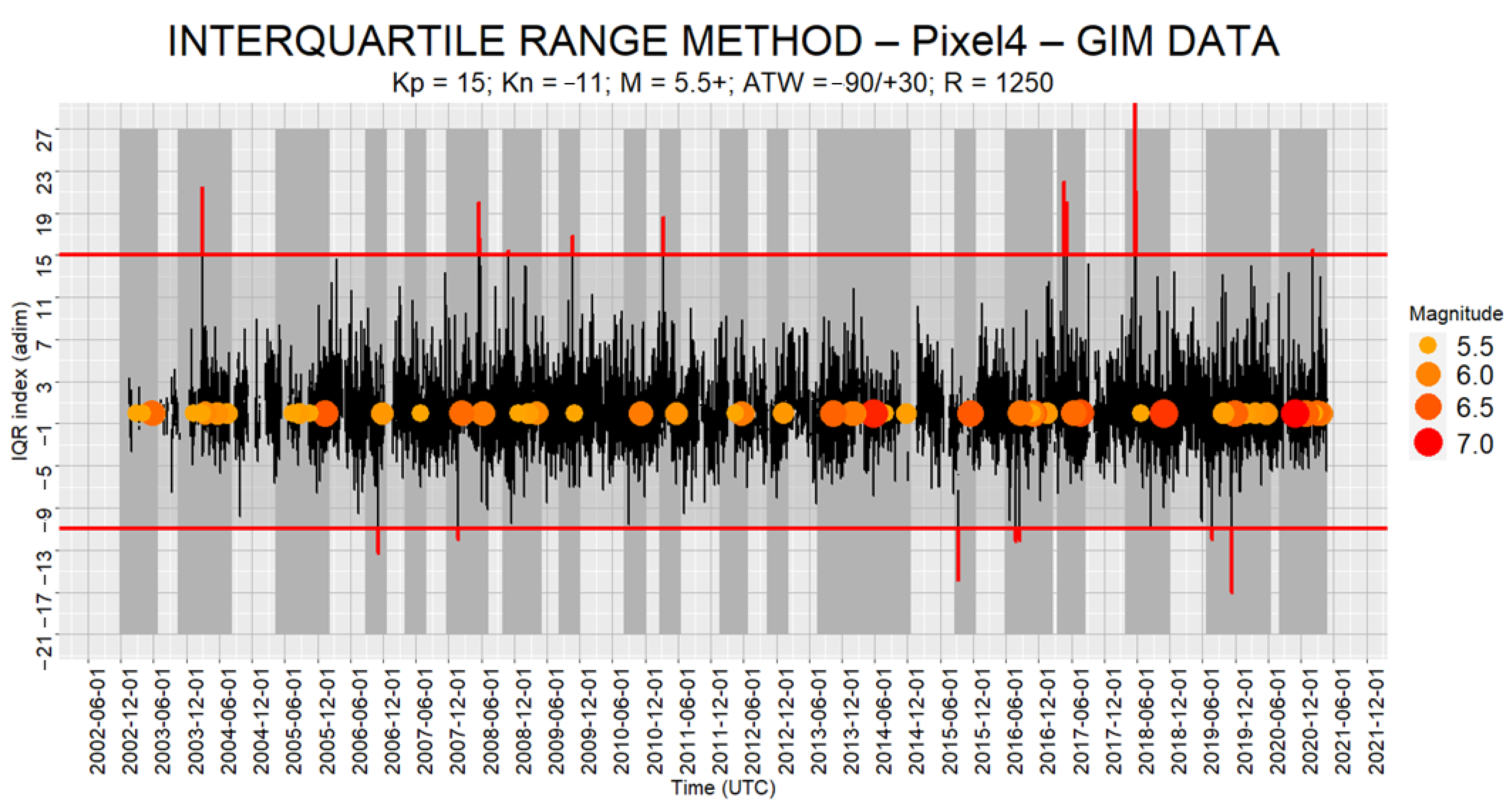
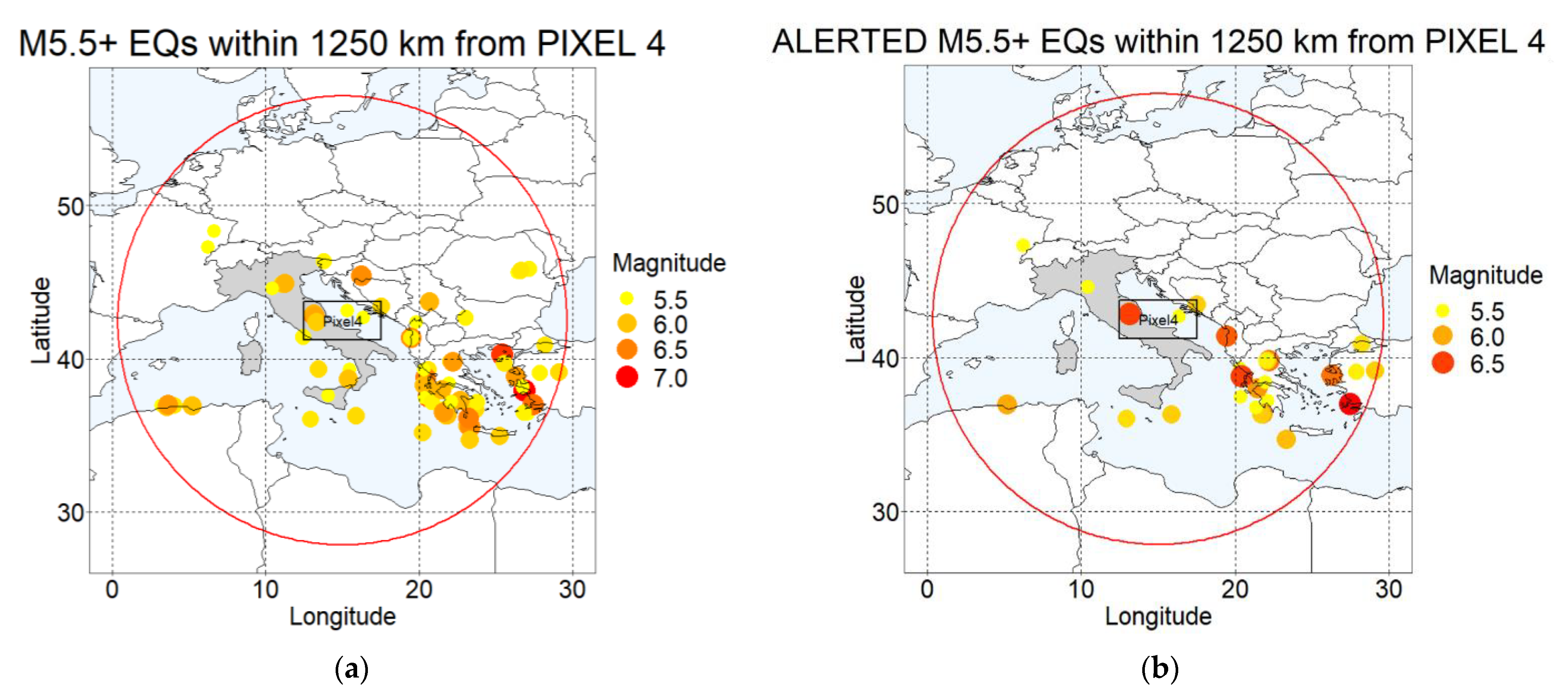
3.2.5. GIM Data IQR Method Optimal Radius: Results within R1250

In

Table 35. IQR method outputs for which the best performance was obtained in the framework of the Pixel 4 GIM-data application within R1250.

Kpos	Kneg	ATW	M	EQs	TP	FP	ATrate	LR+	RP
15	−11	−90/+30	5.5	69	22	0	0.6051	Inf	0.000016

we show input parameters and main results obtained from the analysis within the radius of 1250 km, using the R2200 Kpos and Kneg thresholds.

In comparison to the analysis with R2200 the ATrate decreased from 71.9% to 60.5% and consequently the probability that the 22 TPs are random (stochastic) events (RP) decreased from 0.23% to 16 cases out of 1 million. The number of seismic events included in the area of influence decreased by 27 units (from 96 to 69).

In Figure 19 we show, for pixel 4 within the radius of 1250 km, the IQR index plot combined with the earthquakes occurring in the relative MST domain under investigation.

In Figure 19 the number and intensity of anomalies are the same compared to the case with the radius of 2200 km; the only difference is the lower number of seismic events and consequently the smallest extent in the entire time interval of the ATWs.

In

Table 36. Characterization of the TP detected using the GIM-TEC data recorded within pixel 4 and within the distance of 1250 km from the center of the pixel. Magnitudes in bold highlight the closest event in terms of time to the anomaly detected. EQ dates in bold indicate earthquakes alerted of not for the first time (second or third anomaly occurrence related to the same EQ).

IQR Method—Pixel 4—M5.5+—ATW−90/+30—R1250
TP Detected				Related EQ(s)
#	IQR Index	Date	Type	M	Date	Days from TP	Dist. (km)
1	21.5	28 February 2004	POST-SEISMIC	5.5	23 February 2004	5	874
			PRE-SEISMIC	5.5	1 March 2004	−2	848
			PRE-SEISMIC	5.9	17 March 2004	−18	1128
			PRE-SEISMIC	5.8	23 May 2004	−85	228
2	−13.3	3 November 2006	PRE-SEISMIC	5.7	23 November 2006	−20	741
			PRE-SEISMIC	5.8	24 November 2006	−21	693
3	21.0	7 May 2007	PRE-SEISMIC	5.5	29 June 2007	−53	573
4	−12.0	22 January 2008	PRE-SEISMIC	6.3	14 February 2008	−23	876
			PRE-SEISMIC	6	14 February 2008	−23	901
			PRE-SEISMIC	5.8	20 February 2008	−29	898
5	20.0	19 May 2008	PRE-SEISMIC	6.1	8 June 2008	−20	745
6	16.6	20 May 2008	PRE-SEISMIC	6.1	8 June 2008	−19	745
7	15.4	30 October 2008	PRE-SEISMIC	5.5	23 December 2008	−54	436
8	16.8	22 October 2009	PRE-SEISMIC	5.5	3 November 2009	−12	725
9	15.6	22 October 2009	PRE-SEISMIC	5.5	3 November 2009	−12	725
10	18.6	9 March 2011	PRE-SEISMIC	5.8	19 May 2011	−71	1247
11	−16.0	8 September 2015	PRE-SEISMIC	6.5	17 November 2015	−70	614
12	−11.7	24 July 2016	PRE-SEISMIC	6.2	24 August 2016	−31	148
			PRE-SEISMIC	5.5	24 August 2016	−31	155
13	−12.2	27 July 2016	PRE-SEISMIC	6.2	24 August 2016	−28	148
			PRE-SEISMIC	5.5	24 August 2016	−28	155
14	−12.1	16 August 2016	PRE-SEISMIC	6.2	24 August 2016	−8	148
			PRE-SEISMIC	5.5	24 August 2016	−8	155
			PRE-SEISMIC	5.5	26 October 2016	−71	159
			PRE-SEISMIC	6.1	26 October 2016	−71	160
			PRE-SEISMIC	6.5	30 October 2016	−75	159
15	22.0	20 April 2017	PRE-SEISMIC	6.3	12 June 2017	−53	1037
16	20.0	8 May 2017	PRE-SEISMIC	6.3	12 June 2017	−35	1037
			PRE-SEISMIC	6.6	20 July 2017	−73	1230
17	Inf	23 May 2018	PRE-SEISMIC	5.5	25 June 2018	−33	843
18	16.0	25 May 2018	PRE-SEISMIC	5.5	25 June 2018	−31	843
19	21.0	26 May 2018	PRE-SEISMIC	5.5	25 June 2018	−30	843
20	−12.0	22 July 2019	PRE-SEISMIC	5.8	8 August 2019	−17	1344
			PRE-SEISMIC	5.6	21 September 2019	−61	390
			PRE-SEISMIC	5.7	26 September 2019	−66	1112
21	−17.0	8 November 2019	PRE-SEISMIC	6.4	26 November 2019	−18	391
			PRE-SEISMIC	5.6	22 January 2020	−75	1148
			PRE-SEISMIC	6.8	24 January 2020	−77	2098
			PRE-SEISMIC	5.7	30 January 2020	−83	1381
			PRE-SEISMIC	5.6	30 January 2020	−83	1388
22	15.5	2 February 2021	PRE-SEISMIC	5.5	17 February 2021	−15	747
			PRE-SEISMIC	6.3	3 March 2021	−29	677
			PRE-SEISMIC	5.8	4 March 2021	−30	669
			PRE-SEISMIC	5.6	12 March 2021	−38	658
			PRE-SEISMIC	6	18 March 2021	−44	1042
			PRE-SEISMIC	5.5	27 March 2021	−53	114

the main information of the analysis with R1250 is shown.

As in the previous case, the 22 verified anomalies were mainly of a pre-seismic nature except for no. 1, which was co-seismic (pre- and post-seismic). Using the MST domain M5.5+, R1250 and ATW−90/+30, 42 seismic events were connected to the 22 TPs. A total of 26 of them had magnitudes between 5.5 and 5.9, while 16 of them were M6+ events. The earthquake-anomaly temporal distances varied between −85 and +5 days and the spatial distances between 114 and 1247 km. If we select only the 22 earthquakes closest to the 22 detected seismic-related anomalies (whose magnitudes are in bold) and we exclude the seismic events connected to more than one anomaly (whose dates are in bold), the 22 TPs alerted in total of 15 seismic events.

Figure 20 shows all 69 M5.5+ seismic events occurring in the entire space-time interval under investigation (a) and the 42 seismic events that fall within the selected magnitude-space-time domain “alerted” by the applied IQR method (b).

Comparing from Figure 20 the left (a) and right side (b), the spatial distribution of the alerted events with respect to those that occurred within the domain under investigation appeared to be rather homogeneous, without particular densification.

4. Discussion

In this work, an optimal setting and long-term validation of the methodological inputs used for the detection of earthquake-related anomalies of the ionospheric-Total Electron Content (TEC) was made. The setting was optimized using our own R-coded machine learning techniques capable of combining multi-year time series of TEC satellite data and multi-year time series of seismic catalogues, simulating their behaviors in tens of thousands of possible combinations and classifying them according to criteria established a priori.

The most widely used method to detect ionospheric anomalies, the InterQuartile Range (IQR), was used as a working basis. Its input elements were selected both as a result of an in-depth literature review of the main statistical analyses performed on the topic, and proposed by us following theoretical reasoning validated in the data analysis phase. The input setting and validation were done on TEC time-series obtained from single GNSS receivers or extracted from Global Ionospheric Maps (GIMs) and used for the detection of seismic-related anomalies across the Italian region. The seismic events involved in the analysis concerned seismically active areas up to 2200 km distant from central Italy, including all the countries of the Mediterranean area, from Portugal to Turkey.

Following the results obtained by combining the inputs examined, what we propose are not exportable models, because we assume that some different inputs examined are affected by the physical characteristics of the geographical area analyzed (latitude above all) others by the technical characteristics of the measuring instruments, others by both these factors and still others influence each other (e.g., magnitude and distance from the epicenter). Furthermore, the ionosphere is also subject to unknown noise sources which can produce significant disturbances that can currently only be managed statistically.

Therefore, the first thing we propose is the use of this type of approach, which allows the measurement of the performance of the various inputs and to combine them to derive effective methods every time the geographical position and measurement instruments change.

Measurements of input and method (input combinations) performance, however, served as validation/disprove tests on each single input element proposal. From these, we drew various conclusions and indications valid for applications at mid-latitudes which we discuss below.

Three categories of input were tested: inputs of the IQR index (4 inputs), inputs of the earthquake Magnitude-space-time (MST) domain (4 inputs), thresholds for the detection of anomalies (1991 threshold combination). The inputs of the IQR index evaluated were: daily sliding window, solar activity filter, geomagnetic activity filter and persistence criterion. The evaluation of the inputs of the earthquake MST domain concerned: minimum magnitude, area of influence (optimal radius), depth filter and anomaly time window. The elements making up the 8 inputs (2 or 3 for each of them) generated 816 different combinations of inputs (IQR methods), applied in a diversified way on 10 sites under investigation (areas around 3 GNSS stations and 7 GIM pixels), resulting in 1920 multi-year (mostly nearly 20-year) IQR time-series analyzed. Overall, periods involved were in the time interval from 2001 to 2021. To measure the performance of such a large number of multi-year databases, a synthetic statistical index called LR+ (positive likelihood ratio) was used. As a function of it, through a classification by homogeneous pairs/triples of input elements, the intermediate results of optimal setting of the inputs were obtained, which led to the first conclusions set out below.

Firm conclusions concern IQR inputs daily sliding window (DWS), persistence criterion (P) and depth filter (DF).

• DSW (Daily Sliding Window): the results obtained clearly show that the 27-day moving window is better suited to the detection of TEC anomalies than the 15-day one, regardless of the type of data used (single GNSS receiver or Global ionospheric map).
• P (Persistence criterion): the persistence criterion, tested on a duration of 8 h a day (1/3 of the daily data points) did not prove effective on any of the long-term applications carried out. We conclude that the detection of seismic-ionospheric anomalies can be more efficient looking for punctual rather than persistent phenomena.
• DF (Depth Filter): the depth filter, for which earthquakes with seismic focus depth greater than 50 km were excluded, proved to be effective in about 80% of the cases analyzed. Our results confirm that earthquakes deeper than 50 km are less likely to affect the ionosphere.

The following conclusions require further confirmation.

• GF (Geomagnetic activity Filter): the application of the filter (|Dst| ≤ 20 nT) gave uncertain results on tests with a limited area of influence (Dobrovolsky radius), on both types of data (single receiver and GIM), but excellent results as the area of influence increased. In general, it seems to work where there is a sufficiently high number of seismic events, and we consider this an important value, also because the sites in which it has given the best results also correspond to those in which the best final results are recorded (aqui station and GIM pixels with R ≤ 1000 km), so we recommend its use.
• SF (Solar activity Filter): the proposed solar activity filter, composed of a fixed and a variable threshold (see Section 2.4.2), gave excellent results in the application on the data coming from single GNSS receivers, while it seems to be irrelevant in this intermediate analysis on GIM data. We expect that this is only due to the particular setting of the first approximation thresholds, as in the subsequent analysis with the optimal thresholds it gave some indication of effectiveness (see comments to Figure 18), but to demonstrate it we would need more specific in-depth analysis.

Subsequently, by fixing these input elements, a screened list of 90 IQR time-series was obtained. On these we proceeded to set the optimal thresholds through an iterative process that led to the processing of over 14,000 multi-year IQR time-series and to classify them. On these time-series the random probability (RP) was also calculated, i.e., an index of measurement of the probability that the results obtained are random. The best input combinations were extracted and analyzed from the ranking.

Following the further main conclusions were drawn from this second type of analysis.

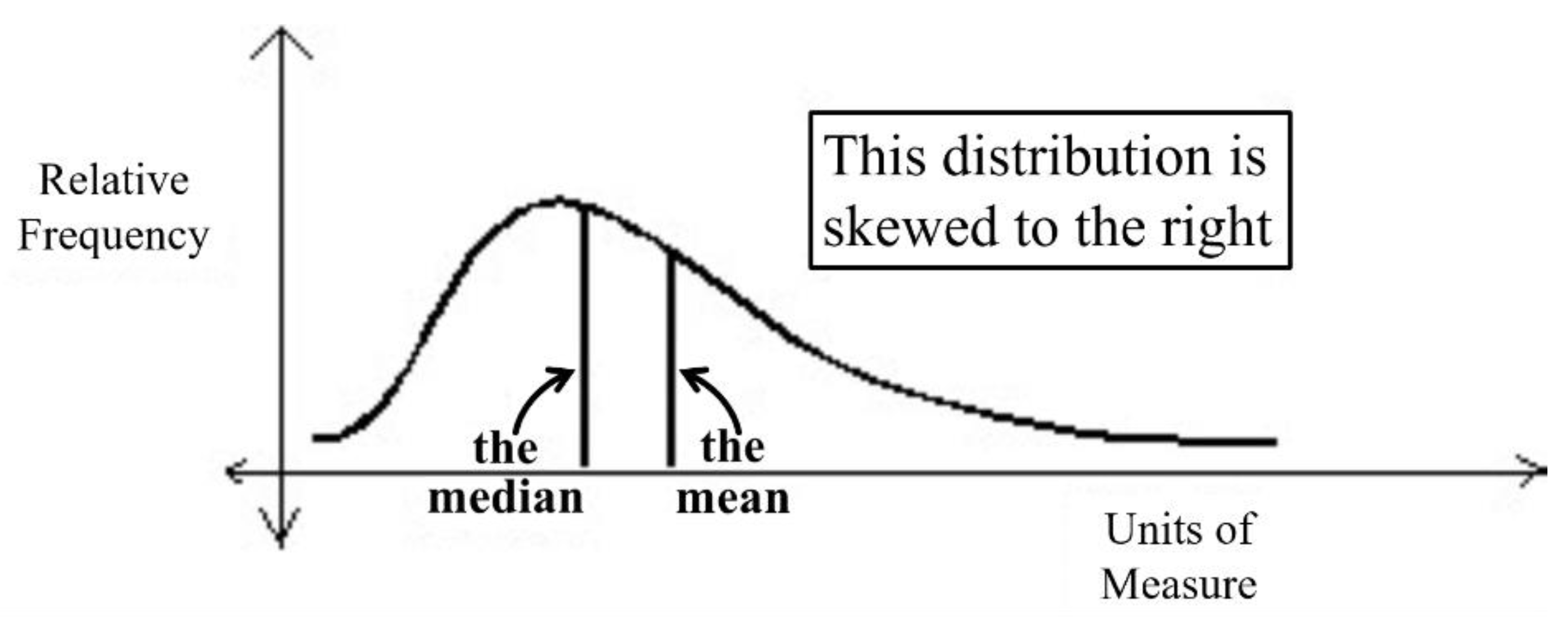
• Kpos & Kneg (thresholds) optimal setting: from the assumption that the comparison samples are non-Gaussian, mainly right-tailed, confirmed by the long-term IQR trends observed tending to develop towards the positive sign, it follows that the thresholds used (positive and negative) should be set independent of each other, because their optimal setting also has a higher tendency to register positive thresholds than negative ones. Furthermore, although the efforts and needs to determine common thresholds for the different observation sites are reasonable, according to our results, the possibility that different threshold levels are necessary to describe such a complex phenomenon cannot be excluded. In fact, in addition to being extremely variable from a space-time point of view, the TEC is also subject to different levels of signal-to-noise ratio depending on the type of observation and on the technical characteristics of the ground stations.
• Single GNSS stations: with the data of the single GNSS stations, from 10 to 20 anomalies were detected in the absence of false positives with random probabilities ranging from 2.4 out of 100 to 2 out of 1 million. Furthermore, the long seismic sequences of 2016 and 2012 were alerted of by the stations of L’Aquila (Italy) and Modena (Italy) by particularly intense anomalies repeated over short days. This, although we are aware of the need to confirm the observations on other sites and to restrict the range of variability of the optimal thresholds applied, leads us to believe that, when the other input parameters are optimally set, data obtained from the individual GNSS receivers are useful for capturing local earthquake-ionospheric effects (Magnitude ≥ 4; Distance ≤ Dobrovolsky radius).
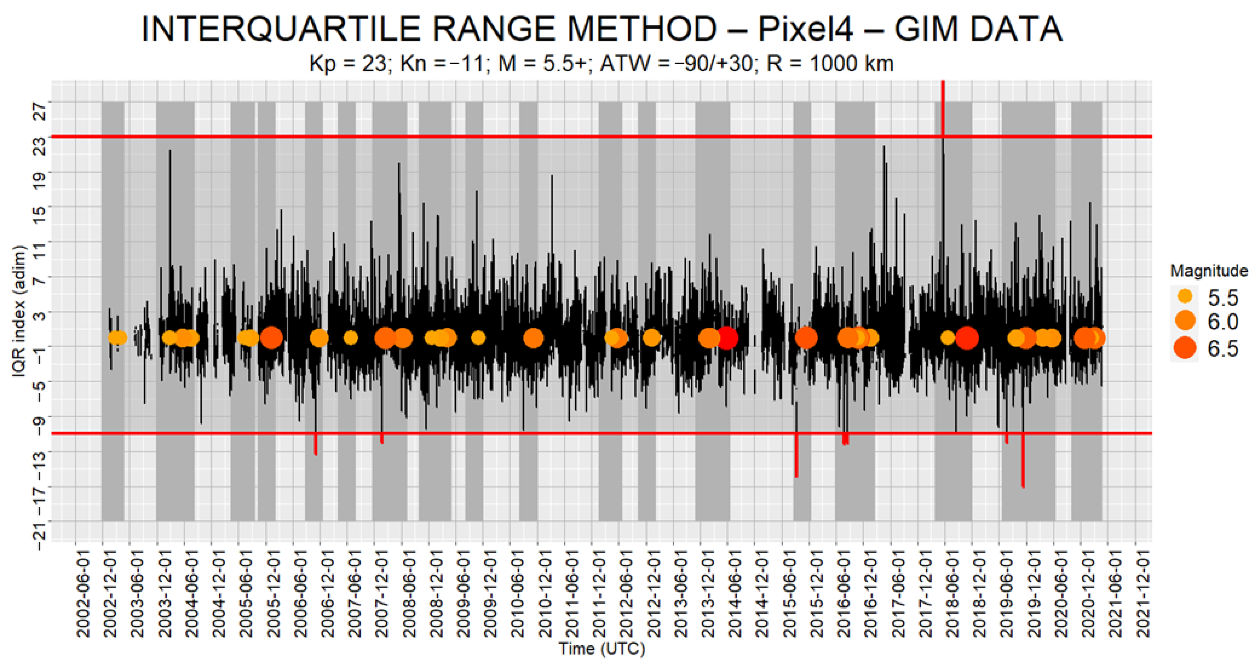
• GIM data: GIM data proved to be particularly effective in detecting large-scale earthquake-ionospheric effects. Although there is a need to validate the observation on other areas, the preliminary results of this type of observation are extremely interesting.

Following the multitude of analyses carried out for the setting of the MST (magnitude-space-time) domain, we propose the use of the following inputs:

–

Magnitude ≥ 5.5;

–

Distance from the center of the pixel less than 1250 km;

–

Hypocenter less than 50 km;

–

Anomaly time window ranging from 90 days before (after) to 30 days after (before) the seismic event (the ionospheric anomaly).

Within this MST domain, the 22 most intense anomalies that were detected were all connected to seismic events. The probability that all 22 anomalies were detected randomly is extremely low (16 cases out of 1 million). 21 out of 22 anomalies were exclusively pre-seismic and 1 was co-seismic (pre- and post-seismic).

A final and general conclusion of our research work is that:

• The optimal setting of the methodological inputs employed in the methods for the identification of TEC co-seismic anomalies through long-term validation represents a valid action strategy.

We also want to underline that (as pointed out by several authors, e.g., [51]) our results strengthen the hypothesis that not all seismic events (even strong ones) produce anomalies and, even if this were not the case, at the current state of research on the subject we are absolutely unable to identify them all (at least not with a single parameter). In fact, for example, our methods did not extract anomalies associated with one of the largest earthquakes to occur in Italy in the time investigated, the Mw = 6.2 L’Aquila 6 April 2009 earthquake, despite one GNSS station being very close to the epicenter and the investigated pixel 4 of GIM contained the epicenter as well. At the same time, we want to highlight that we do not consider this a relevant problem, as in the current state of research, the prediction of even a single seismic event would be an unprecedented result. Therefore, we believe it is appropriate to direct our efforts in this direction.

The results obtained in this work are useful to circumscribe the huge number of approaches developed to date on the study of ionospheric seismic-connected anomalies and could be used as a first working basis on which to build a further detailed model or a real-time test phase of the method, or a model that calls into question additional seismic-connected parameters. The possibility of combining additional parameters for which multi-year analyses have been carried out, such as thermal infrared emission (TIR), could be assessed in order to evaluate how and to what extent a multi-parametric approach can lead to the definition of more specific alert levels or to the reduction of the alerted space-time volumes (compared with a single parameter approach) as proposed in the framework of the Time-Dependent Assessment of Seismic Hazard (T-DASH; [59,70]) and in other recent scientific publications (e.g., [71]).

References

1. Leonard, R.S.; Barnes, R.A. Observation of ionospheric disturbances following the Alaska earthquake. J. Geophys. Res. 1965, 70, 1250–1253. [Google Scholar] [CrossRef]
2. Davies, K.; Baker, D.M. Ionospheric effects observed around time of Alaskan earthquake of 28 March 1964. J. Geophys. Res. 1965, 70, 2251–2253. [Google Scholar] [CrossRef]
3. Uyeda, S.; Nagao, T. Historical Development of Pre-Earthquake Phenomena Studies. In Pre-Earthquake Processes. A Multidisciplinary Approach to Earthquake Prediction Studies; Ouzounov, D., Pulinets, S., Hattori, K., Taylor, P., Eds.; John Wiley & Sons: Hoboken, NJ, USA, 2018; pp. 19–39. [Google Scholar] [CrossRef]
4. Park, S.K.; Johnston, M.J.S.; Madden, T.R.; Morgan, F.D.; Morrison, H.F. Electromagnetic precursors to earthquakes in the Ulf band: A review of observations and mechanisms. Rev. Geophys. 1993, 31, 117–132. [Google Scholar] [CrossRef]
5. Geller, R.J. Earthquake prediction: A critical review. Geophys. J. Int. 1997, 131, 425–450. [Google Scholar] [CrossRef]
6. Johnston, M.J.S. Review of Electric and Magnetic fields Accompanying Seismic and Volcanic Activity. Surv. Geophys. 1997, 18, 441–476. [Google Scholar] [CrossRef]
7. Tronin, A.A. Remote sensing and earthquakes: A review. Phys. Chem. Earth Parts A/B/C 2006, 31, 138–142. [Google Scholar] [CrossRef]
8. Helman, D.S. Seismic electric signals (SES) and earthquakes: A review of an updated VAN method and competing hypotheses for SES generation and earthquake triggering. Phys. Earth Planet. Inter. 2020, 302, 106484. [Google Scholar] [CrossRef]
9. Sorokin, V.M.; Chmyrev, V.M.; Hayakawa, M. A Review on Electrodynamic Influence of Atmospheric Processes to the Ionosphere. Open J. Earthq. Res. 2020, 09, 113–141. [Google Scholar] [CrossRef]
10. Picozza, P.; Conti, L.; Sotgiu, A. Looking for Earthquake Precursors From Space: A Critical Review. Front. Earth Sci. 2021, 9, 676775. [Google Scholar] [CrossRef]
11. Conti, L.; Picozza, P.; Sotgiu, A. A Critical Review of Ground Based Observations of Earthquake Precursors. Front. Earth Sci. 2021, 9, 676766. [Google Scholar] [CrossRef]
12. Chen, H.; Han, P.; Hattori, K. Recent Advances and Challenges in the Seismo-Electromagnetic Study: A Brief Review. Remote Sens. 2022, 14, 5893. [Google Scholar] [CrossRef]
13. Available online: https://directory.eoportal.org/web/eoportal/satellite-missions/c-missions/cses (accessed on 13 August 2022).
14. Zhima, Z.; Yan, R.; Lin, J.; Wang, Q.; Yang, Y.; Lv, F.; Huang, J.; Cui, J.; Liu, Q.; Zhao, S.; et al. The Possible Seismo-Ionospheric Perturbations Recorded by the China-Seismo-Electromagnetic Satellite. Remote Sens. 2022, 14, 905. [Google Scholar] [CrossRef]
15. Available online: https://demeter.cnes.fr/en/home-76 (accessed on 13 August 2022).
16. Parrot, M.; Li, M. Demeter results related to seismic activity. URSI Radio Sci. Bull. 2015, 2015, 18–25. [Google Scholar] [CrossRef]
17. Bergeot, N.; Tsagouri, I.; Bruyninx, C.; Legrand, J.; Chevalier, J.-M.; Defraigne, P.; Baire, Q.; Pottiaux, E. The influence of space weather on ionospheric total electron content during the 23rd solar cycle. J. Space Weather Space Clim. 2013, 3, A25. [Google Scholar] [CrossRef]
18. Liu, L.; Chen, Y. Statistical analysis of solar activity variations of total electron content derived at Jet Propulsion Laboratory from GPS observations. J. Geophys. Res. 2009, 114, A10311. [Google Scholar] [CrossRef]
19. Colonna, R.; Tramutoli, V. A New Model of Solar Illumination of Earth’s Atmosphere during Night-Time. Earth 2021, 2, 191–207. [Google Scholar] [CrossRef]
20. Liu, J.Y.; Chuo, Y.J.; Shan, S.J.; Tsai, Y.B.; Chen, Y.I.; Pulinets, S.A.; Yu, S.B. Pre-earthquake ionospheric anomalies registered by continuous GPS TEC measurements. Ann. Geophys. 2004, 22, 1585–1593. [Google Scholar] [CrossRef]
21. Guo, J.; Shi, K.; Liu, X.; Sun, Y.; Li, W.; Kong, Q. Singular spectrum analysis of ionospheric anomalies preceding great earthquakes: Case studies of Kaikoura and Fukushima earthquakes. J. Geodyn. 2019, 124, 1–13. [Google Scholar] [CrossRef]
22. Kon, S.; Nishihashi, M.; Hattori, K. Ionospheric anomalies possibly associated with M ≥ 6.0 earthquakes in the Japan area during 1998–2010: Case studies and statistical study. J. Asian Earth Sci. 2011, 41, 410–420. [Google Scholar] [CrossRef]
23. Le, H.; Liu, J.Y.; Liu, L. A statistical analysis of ionospheric anomalies before 736M6.0+ earthquakes during 2002–2010. J. Geophys. Res. 2011, 116, A02303. [Google Scholar] [CrossRef]
24. Liu, J.; Chen, C.H.; Tsai, H.-F. A Statistical Study on Seismo-Ionospheric Anomalies of the Total Electron Content for the Period of 56 M≥6.0 Earthquakes Occurring in China during 1998–2012. Chin. J. Space Sci. 2013, 33, 258–269. [Google Scholar]
25. Liu, J.Y.; Chen, C.H.; Tsai, H.F. A statistical study on seismoionospheric precursors of the total electron content associated with 146 M 6.0 earthquakes in Japan during 1998–2011. In Earthquake Prediction Studies: Seismo Electromagnetics; Hayagawa, M., Ed.; TERRAPUB: Tokyo, Japan, 2013; pp. 17–30. [Google Scholar]
26. Şentürk, E.; Çepni, M.S. A statistical analysis of seismo-ionospheric TEC anomalies before 63 Mw ≥ 5.0 earthquakes in Turkey during 2003–2016. Acta Geophys. 2018, 66, 1495–1507. [Google Scholar] [CrossRef]
27. Shah, M.; Ahmed, A.; Ehsan, M.; Khan, M.; Tariq, M.A.; Calabia, A.; Rahman, Z.U. Total electron content anomalies associated with earthquakes occurred during 1998–2019. Acta Astronaut. 2020, 175, 268–276. [Google Scholar] [CrossRef]
28. Available online: http://www.ionolab.org/index.php?page=ionolabtec&language=en (accessed on 14 August 2022).
29. Arikan, F.; Erol, C.B.; Arikan, O. Regularized estimation of vertical total electron content from Global Positioning System data. J. Geophys. Res. Atmos. 2003, 108, 1469. [Google Scholar] [CrossRef]
30. Sezen, U.; Arikan, F.; Arikan, O.; Ugurlu, O.; Sadeghimorad, A. Online, automatic, near-real time estimation of GPS-TEC: IONOLAB-TEC. Space Weather 2013, 11, 297–305. [Google Scholar] [CrossRef]
31. Arikan, F.; Nayir, H.; Sezen, U.; Arikan, O. Estimation of single station interfrequency receiver bias using GPS-TEC. Radio Sci. 2008, 43, 4. [Google Scholar] [CrossRef]
32. Available online: https://cddis.nasa.gov/archive/gnss/products/ionex/ (accessed on 14 August 2022).
33. Dobrovolsky, I.P.; Zubkov, S.I.; Miachkin, V.I. Estimation of the size of earthquake preparation zones. Pure Appl. Geophys. 1979, 117, 1025–1044. [Google Scholar] [CrossRef]
34. Liu, J.-Y.; Chen, Y.-I.; Jhuang, H.-K.; Lin, Y.-H. Ionospheric foF2 and TEC Anomalous Days Associated with M >= 5.0 Earthquakes in Taiwan during 1997–1999. Terr. Atmos. Ocean. Sci. 2004, 15, 371–383. [Google Scholar] [CrossRef]
35. Liu, J.Y.; Chen, Y.I.; Chuo, Y.J.; Chen, C.S. A statistical investigation of preearthquake ionospheric anomaly. J. Geophys. Res. Atmos. 2006, 111, A05304. [Google Scholar] [CrossRef]
36. Liu, J.Y.; Chen, Y.I.; Chen, C.H.; Liu, C.Y.; Chen, C.Y.; Nishihashi, M.; Li, J.Z.; Xia, Y.Q.; Oyama, K.I.; Hattori, K.; et al. Seismoionospheric GPS total electron content anomalies observed before the 12 May 2008Mw7.9 Wenchuan earthquake. J. Geophys. Res. Earth Surf. 2009, 114, A04320. [Google Scholar] [CrossRef]
37. Liu, J.Y.; Le, H.; Chen, Y.I.; Chen, C.H.; Liu, L.; Wan, W.; Su, Y.Z.; Sun, Y.Y.; Lin, C.H.; Chen, M.Q. Observations and simulations of seismoionospheric GPS total electron content anomalies before the 12 January 2010M7 Haiti earthquake. J. Geophys. Res. Atmos. 2011, 116, A04302. [Google Scholar] [CrossRef]
38. Liu, C.-Y.; Liu, J.-Y.; Chen, Y.-I.; Qin, F.; Chen, W.-S.; Xia, Y.-Q.; Bai, Z.-Q. Statistical analyses on the ionospheric total electron content related to M ≥ 6.0 earthquakes in China during 1998–2015. Terr. Atmos. Ocean. Sci. 2018, 29, 485–498. [Google Scholar] [CrossRef]
39. Li, J.; Meng, G.; Wang, M.; Liao, H.; Shen, X. Investigation of ionospheric TEC changes related to the 2008 Wenchuan earthquake based on statistic analysis and signal detection. Earthq. Sci. 2009, 22, 545–553. [Google Scholar] [CrossRef]
40. Jiang, W.; Ma, Y.; Zhou, X.; Li, Z.; An, X.; Wang, K. Analysis of Ionospheric Vertical Total Electron Content before the 2014 Mw8.2 Chile Earthquake. Preprints 2017, 2017040060. [Google Scholar] [CrossRef]
41. Sharma, G.; Champati Ray, P.K.; Kannaujiya, S. Ionospheric Total Electron Content for Earthquake Precursor Detection. In Remote Sensing of Northwest Himalayan Ecosystems; Navalgund, R., Kumar, A., Nandy, S., Eds.; Springer: Singapore, 2019. [Google Scholar] [CrossRef]
42. Sasmal, S.; Chowdhury, S.; Kundu, S.; Politis, D.Z.; Potirakis, S.M.; Balasis, G.; Hayakawa, M.; Chakrabarti, S.K. Pre-Seismic Irregularities during the 2020 Samos (Greece) Earthquake (M = 6.9) as Investigated from Multi-Parameter Approach by Ground and Space-Based Techniques. Atmosphere 2021, 12, 1059. [Google Scholar] [CrossRef]
43. Figure from: Illinois State University Mathematics Department. Available online: https://math.illinoisstate.edu/day/courses/old/312/notes/onevar/onevar04.html (accessed on 18 August 2022).
44. Tariq, M.A.; Shah, M.; Li, Z.; Wang, N.; Iqbal, T.; Liu, L. Lithosphere ionosphere coupling associated with three earthquakes in Pakistan from GPS and GIM TEC. J. Geodyn. 2021, 147, 101860. [Google Scholar] [CrossRef]
45. Guo, J.; Li, W.; Yu, H.; Liu, Z.; Zhao, C.; Kong, Q. Impending ionospheric anomaly preceding the Iquique Mw8.2 earthquake in Chile on 2014 April 1. Geophys. J. Int. 2015, 203, 1461–1470. [Google Scholar] [CrossRef]
46. Şentürk, E.; Livaoğlu, H.; Çepni, M.S. A Comprehensive Analysis of Ionospheric Anomalies before the Mw7·1 Van Earthquake on 23 October 2011. J. Navig. 2019, 72, 702–720. [Google Scholar] [CrossRef]
47. Colonna, R.; Filizzola, C.; Genzano, N.; Lisi, M.; Pergola, N.; Tramutoli, V. Long-term analysis of the Ionospheric-Total Electron Content (TEC) parameter for the detection of anomalous behaviours potentially related to seismic activity. In Proceedings of the EGU General Assembly Conference Abstracts, Online, 19–30 April 2021. EGU21-13730. [Google Scholar] [CrossRef]
48. Liu, L.; Wan, W.; Ning, B.; Zhang, M.-L. Climatology of the mean total electron content derived from GPS global ionospheric maps. J. Geophys. Res. Atmos. 2009, 114, A06308. [Google Scholar] [CrossRef]
49. Available online: https://omniweb.gsfc.nasa.gov/form/dx1.html (accessed on 19 August 2022).
50. Yan, X.; Yu, T.; Shan, X.; Xia, C. Ionospheric TEC disturbance study over seismically region in China. Adv. Space Res. 2017, 60, 2822–2835. [Google Scholar] [CrossRef]
51. De Santis, A.; Marchetti, D.; Pavón-Carrasco, F.J.; Cianchini, G.; Perrone, L.; Abbattista, C.; Alfonsi, L.; Amoruso, L.; Campuzano, S.A.; Carbone, M.; et al. Precursory worldwide signatures of earthquake occurrences on Swarm satellite data. Sci. Rep. 2019, 9, 20287. [Google Scholar] [CrossRef]
52. Hayakawa, M.; Molchanov, O.A. Seismo Electromagnetics: Lithosphere-Atmosphere-Ionosphere Coupling; Terrapub: Tokyo, Japan, 2002; Volume 477. [Google Scholar]
53. Pulinets, S.A.; Boyarchuk, K. Ionospheric Precursors of Earthquakes; Springer: Berlin/Heidelberg, Germany, 2004. [Google Scholar]
54. Perrone, L.; De Santis, A.; Abbattista, C.; Alfonsi, L.; Amoruso, L.; Carbone, M.; Cesaroni, C.; Cianchini, G.; De Franceschi, G.; De Santis, A.; et al. Ionospheric anomalies detected by ionosonde and possibly related to crustal earthquakes in Greece. Ann. Geophys. 2018, 36, 361–371. [Google Scholar] [CrossRef]
55. Debnath, A. Analysis of anomalous ionospheric total electron content variation for earthquakes in South East Asian region with IGS network. Indian J. Radio Space Phys. IJRSP 2020, 49, 28–32. [Google Scholar]
56. Perrone, L.; Korsunova, L.P.; Mikhailov, A.V. Ionospheric precursors for crustal earthquakes in Italy. Ann. Geophys. 2010, 28, 941–950. [Google Scholar] [CrossRef]
57. Ippolito, A.; Perrone, L.; De Santis, A.; Sabbagh, D. Ionosonde Data Analysis in Relation to the 2016 Central Italian Earthquakes. Geosciences 2020, 10, 354. [Google Scholar] [CrossRef]
58. He, Y.; Zhao, X.; Yang, D.; Wu, Y.; Li, Q. A study to investigate the relationship between ionospheric disturbance and seismic activity based on Swarm satellite data. Phys. Earth Planet. Inter. 2022, 323, 106826. [Google Scholar] [CrossRef]
59. Tramutoli, V.; Vallianatos, F. Foreword: Advances in Multi-Parametric, Time-Dependent Assessment of Seismic Hazard and Earthquakes Forecast. Ann. Geophys. 2020, 63, PA555. Available online: https://www.annalsofgeophysics.eu/index.php/annals/article/view/8594 (accessed on 25 August 2022). [CrossRef]
60. Genzano, N.; Filizzola, C.; Hattori, K.; Pergola, N.; Tramutoli, V. Statistical Correlation Analysis between Thermal Infrared Anomalies Observed from MTSATs and Large Earthquakes Occurred in Japan (2005–2015). J. Geophys. Res. Solid Earth 2021, 126, e2020JB020108. [Google Scholar] [CrossRef]
61. Ke, F.; Wang, Y.; Wang, X.; Qian, H.; Shi, C. Statistical analysis of seismo-ionospheric anomalies related to Ms > 5.0 earthquakes in China by GPS TEC. J. Seism. 2016, 20, 137–149. [Google Scholar] [CrossRef]
62. Yan, R.; Parrot, M.; Pinçon, J.-L. Statistical Study on Variations of the Ionospheric Ion Density Observed by DEMETER and Related to Seismic Activities. J. Geophys. Res. Space Phys. 2017, 122, 12421–12429. [Google Scholar] [CrossRef]
63. Marchetti, D.; De Santis, A.; Campuzano, S.A.; Zhu, K.; Soldani, M.; D’Arcangelo, S.; Orlando, M.; Wang, T.; Cianchini, G.; Di Mauro, D.; et al. Worldwide Statistical Correlation of Eight Years of Swarm Satellite Data with M5.5+ Earthquakes: New Hints about the Preseismic Phenomena from Space. Remote Sens. 2022, 14, 2649. [Google Scholar] [CrossRef]
64. Chen, Y.-I.; Huang, C.-S.; Liu, J.-Y. Statistical evidences of seismo-ionospheric precursors applying receiver operating characteristic (ROC) curve on the GPS total electron content in China. J. Asian Earth Sci. 2015, 114, 393–402. [Google Scholar] [CrossRef]
65. Mulic, M.; Natras, R. Ionosphere TEC Variations Over Bosnia and Herzegovina Using GNSS Data. In New Advanced GNSS and 3D Spatial Techniques; Lecture Notes in Geoinformation and Cartography; Cefalo, R., Zieliński, J., Barbarella, M., Eds.; Springer: Cham, Switzerland, 2018. [Google Scholar] [CrossRef]
66. Valerio, T.; Corrado, R.; Carolina, F.; Genzano, N.; Lisi, M.; Paciello, R.; Pergola, N. One year of RST based satellite thermal monitoring over two Italian seismic areas. Boll. Geofis. Teor. Appl. 2015, 56, 275–294. [Google Scholar] [CrossRef]
67. Valerio, T.; Corrado, R.; Carolina, F.; Genzano, N.; Lisi, M.; Pergola, N. From visual comparison to Robust Satellite Techniques: 30 years of thermal infrared satellite data analyses for the study of earthquake preparation phases. Boll. Geofis. Teor. Appl. 2015, 56, 167–202. [Google Scholar] [CrossRef]
68. Available online: www.seismicportal.eu (accessed on 31 August 2022).
69. Godey, S.; Bossu, R.; Guilbert, J.; Mazet-Roux, G. The Euro-Mediterranean Bulletin: A Comprehensive Seismological Bulletin at Regional Scale. Seism. Res. Lett. 2006, 77, 460–474. [Google Scholar] [CrossRef]
70. Genzano, N.; Filizzola, C.; Lisi, M.; Pergola, N.; Tramutoli, V. Toward the development of a multi parametric system for a short-term assessment of the seismic hazard in Italy. Ann. Geophys. 2020, 63, PA550. [Google Scholar] [CrossRef]
71. Parrot, M.; Tramutoli, V.; Liu, T.J.Y.; Pulinets, S.; Ouzounov, D.; Genzano, N.; Lisi, M.; Hattori, K.; Namgaladze, A. Atmospheric and ionospheric coupling phenomena associated with large earthquakes. Eur. Phys. J. Spéc. Top. 2021, 230, 197–225. [Google Scholar] [CrossRef]
Figure 1. Flowchart of the entire procedure developed in the manuscript. Definition of the acronyms used in the figure: TEC = Total Electron Content; GIM = Global Ionospheric Maps; IQR = Inter-quartile Range; MST = Magnitude-Space-Time; EQ = Earthquake; LR+ = Positive Likelihood Ratio; R = Radius; RP = Random Probability; ATW = Anomaly Time Window; M = Magnitude; Kpos = Positive Threshold; Kneg = Negative Threshold.
Geosciences 13 00150 g001
Figure 2. Example of comparison between TEC data at different time resolutions (30 s and 60 min).
Geosciences 13 00150 g002
Figure 3. Geographical location of the GNSS network stations used in the analysis (blue triangles).
Geosciences 13 00150 g003
Figure 4. The 8 GIM pixels covering the Italian area analyzed.
Geosciences 13 00150 g004
Figure 5. Median and mean behavior in right-skewed distribution [43].
Geosciences 13 00150 g005
Figure 6. Plots of the aqui, mops and unpg (a) and of the GIM pixel (b) IQRINDEXES. The black line represents the IQRINDEX, the vertical red lines represent the related anomalies and the horizontal red lines are the first approximation thresholds (Kpos and Kneg values).
Geosciences 13 00150 g006
Figure 7. F10.7 index during the entire period under investigation (2001–2021).
Geosciences 13 00150 g007
Figure 8. Location and magnitude of the earthquakes occurring around the aqui receiver from 1 January 2001 to 31 December 2019 within 150 km or RD (a) and in the 8 GIM pixels from 3 November 2002 to 30 June 2021 (b). The magnitudes are scaled both in size and colour to be easier to read.
Geosciences 13 00150 g008
Figure 9. Location and magnitude of the earthquakes occurring within 1000 km (a) and 2200 km (b) from the central coordinates of pixel 4 (Lat 42.5°; Long 15°) from November 2002 to July 2021. The magnitudes are scaled both in size and colour to be easier to read.
Geosciences 13 00150 g009
Figure 10. LR+ rank sums of the IQR input variables applied on the 7 GIM pixels covering Italy within RD. The inputs ranked are the following: DSW = Daily Sliding Window; SF = Solar activity Filter; GF = Geomagnetic activity Filter; P = Persistence criterion; ATW = Anomaly Time Window; M = Magnitude.
Geosciences 13 00150 g010
Figure 11. Depth Filter (DF) LR+ rank sums of the IQR methods applied on Pixel 6 and Pixel 8.
Geosciences 13 00150 g011
Figure 12. LR+ rank sums of the IQR method input variables applied on pixel 4 with R = 1000 km (a) and R = 2200 km (b). The inputs under investigation are the following: DSW = Daily Sliding Window; SF = Solar activity Filter; GF = Geomagnetic activity Filter; P = Persistence criterion; ATW = Anomaly Time Window; M = Magnitude.
Geosciences 13 00150 g012
Figure 13. aqui station IQR index trend compared to seismic activity within 150 km/RD. The black line represents the IQR index, the vertical red lines represent the TP anomalies detected, the horizontal red lines the upper and lower thresholds. On the horizontal axis the EQs occurred vs. time in the MST domain under investigation are reported. The vertical grey ribbons delimit the ATW. In the case of the 24 December 2004 post-seismic anomaly the previous and next IQR index data are not available due to insufficient values in the comparison sample. The R program in this case, not being able to draw any line, adds the value as a geometry point.
Geosciences 13 00150 g013
Figure 14. mops station IQR index trend compared to seismic activity within 150 km/RD. The black line represents the IQR index, the vertical red lines represent the TP anomalies detected, the horizontal red lines the upper and lower thresholds. On the horizontal axis the EQs occurred vs. time in the MST domain under investigation are reported. The vertical grey ribbons delimit the ATW.
Geosciences 13 00150 g014
Figure 15. unpg station IQR index trend compared to seismic activity within 150 km/RD. The black line represents the IQR index, the vertical red lines represent the TP anomalies detected, the horizontal red lines the upper and lower thresholds. On the horizontal axis the EQs occurred vs. time in the MST domain under investigation are reported. The vertical grey ribbons delimit the ATW.
Geosciences 13 00150 g015
Figure 16. Pixel 4 IQR index trend compared to seismic activity within R1000. The black line represents the IQR index, the vertical red lines represent the TP anomalies detected, the horizontal red lines the upper and lower thresholds. On the horizontal axis the EQs occurred vs. time in the MST domain under investigation are reported. The vertical grey ribbons delimit the ATW.
Geosciences 13 00150 g016
Figure 17. Pixel 4 IQR index trend compared to seismic activity within R2200. The black line represents the IQR index, the vertical red lines represent the TP anomalies detected, the horizontal red lines the upper and lower thresholds. On the horizontal axis the EQs occurred vs. time in the MST domain under investigation are reported. The vertical grey ribbons delimit the ATW.
Geosciences 13 00150 g017
Figure 18. Pixel 4 IQR index trend compared to seismic activity within the distance of 1000 km (top plot) and 2200 km (bottom plot) from the center of the pixel. The black line represents the IQR index, the vertical red lines represent the TP anomalies detected, the horizontal red lines the upper and lower thresholds. On the horizontal axis the EQs occurred vs. time in the MST domain under investigation are reported. The vertical grey ribbons delimit the ATW.
Geosciences 13 00150 g018
Figure 19. Pixel 4 IQR index trend compared to seismic activity within R1250. The black line represents the IQR index, the vertical red lines represent the TP anomalies detected, the horizontal red lines the upper and lower thresholds. On the horizontal axis the EQs occurred vs. time in the MST domain under investigation are reported. The vertical grey ribbons delimit the ATW.
Geosciences 13 00150 g019
Figure 20. Location and magnitude of the 69 M5.5+ EQs occurring within 1250 km of the center of pixel 4 (a) and of the 42 alerted of by the applied methodology (b).
Geosciences 13 00150 g020