Article

Investigating the Influence of a Pre-Existing Shear Band on the Seismic Response of Ideal Step-like Slopes Subjected to Weak Motions: Preliminary Results

Department of Civil, Environmental, Land, Building Engineering and Chemistry (DICATECh), Technical University of Bari, Via Orabona 4, 70125 Bari, Italy
*
Author to whom correspondence should be addressed.
Geosciences 2023, 13(5), 148; https://doi.org/10.3390/geosciences13050148
Submission received: 11 April 2023 / Revised: 10 May 2023 / Accepted: 11 May 2023 / Published: 15 May 2023

Abstract

:
The assessment of slope susceptibility to seismically-induced displacements receives wide attention in the geotechnical earthquake engineering field, but the alteration of the seismic wave inside the slope and at the ground surface due to the presence of a shear band confining a quiescent landslide body is rarely investigated. This paper describes the preliminary results of the numerical analysis of two step-like FE models, reproducing a gentle slope and steep cutting subjected to weak earthquakes, thus focusing on seismic wave amplification processes only. The results show that the higher the thickness of the weakened zone, the higher the maximum value of the amplification factors predicted at the ground surface. For gentle slopes affected by a landslide body confined by a thick shear band, the highest amplification factors are expected in the longer period range of 0.7–1.1 s, while the highest level of amplification is achieved in the intermediate period interval of 0.4–0.8 s in the case of steep slopes. In addition, the parasitic vertical component of acceleration can be considerably amplified beyond the crest and at the toe of the slope for increasing band thickness, especially in the case of steep topography, for which the effects of the shear band morphology enhance those related to the topographic profile. Finally, the fundamental frequency of the sloping deposit is not particularly affected by the presence of the shear band, while the amplitude of the amplification function at the fundamental frequency is clearly related to its thickness.

1. Introduction

Ground response analysis is a key tool in seismic hazard assessment, as the reference ground motion (i.e., at the outcropping bedrock with a flat surface) can be different from that recorded at a nearby site in terms of frequency content, amplitude, duration and polarisation due to local topographic and stratigraphic conditions (e.g., [1]). Previous seismic site response investigations have focused on: (i) the heterogeneity of the deposit with depth and the soil nonlinearity (e.g., [2,3,4,5,6,7]), (ii) the variability of the soil mechanical properties and input motion characteristics (e.g., [8,9,10,11,12,13,14,15,16,17]), (iii) the ground surface topography (e.g., [18,19,20,21,22,23,24,25,26,27]), (iv) the buried morphologies (e.g., [28,29,30]) and (v) the numerical code and approach employed in the simulations (e.g., [31,32,33,34,35,36,37,38]).
When studying the seismic behaviour of a slope affected by a landslide mechanism, most researchers have investigated the interaction between seismic waves and fully-developed landslide bodies, mainly focusing on the evaluation of slope susceptibility to seismically-induced displacements (e.g., [39,40,41,42,43,44,45,46]). In these studies, the entire sliding mass is assumed to be characterised by different physical and mechanical properties with respect to the surrounding stable deposit. However, in some cases, the landslide process may determine the alteration of the soil mechanical properties only at the shear band location as an effect of the shear strain localisation, inducing the degradation of both strength and stiffness in a narrow zone confining the landslide body (e.g., [47,48,49,50]). Therefore, the propagation of seismic waves into a slope could be potentially affected by the presence of a weakened shear band, which may modify the response at the ground surface even during weak earthquake motions. Furthermore, some studies have shown the characteristic directivity of the slope dynamic response to seismic shaking on the basis of geological, geophysical and in situ investigations (e.g., [51,52,53,54,55]). Moreover, a sloping surface can generate a parasitic vertical component of acceleration even for input motions characterised by horizontally polarised waves due to the reflection of the incoming waves from the inclined slope surface [19,56].
Within this framework, the paper presents a set of two-dimensional (2D) finite element (FE) dynamic analyses of ideal slopes in soft soils, including a landslide body confined by a pre-existing weakened shear band. The main purpose is to evaluate the effect of the presence of the disturbed material in the shear band on the seismic response of step-like slope models, mainly focusing on aspects merely related to the seismic wave amplification processes. Indeed, the interactions between the seismic motion and the landslide body, in terms of earthquake-induced displacements causing the activation or the reactivation of the existing landslide mechanism, are beyond the scope of this paper. For this reason, providing that the earthquake loading is expected not to re-activate the sliding mechanism, weak input motions are adopted in the simulations by scaling them to very low peak acceleration. This assumption reasonably allows the adoption of a simple linear visco-elastic constitutive model to simulate the behaviour of the slope soils implemented in the analysis.
For each slope model, the results of the numerical simulations are described in terms of (i) 2D contours of the peak ground acceleration (PGA) of both horizontal and vertical components, to assess the effect of the weakened zone at ground surface and within the slope; (ii) profiles of amplification factors (Afs) (i.e., the ratio between quantities referred to the free-field and the outcrop signals, as described later on), at the ground surface, commonly used as a supporting tool for urban, emergency planning and seismic risk mitigation studies [14,57,58]; (iii) ground motion polarisation plots, to highlight the effect of the pre-existing shear band on the directivity of the surface motion in the vertical plane; (iv) response spectra of the ground surface pseudo-acceleration, typically employed for the design of above-surface structures and infrastructures, in comparison to the 1D response to highlight the influence of the shear band morphology; (v) amplification functions in the frequency domain, widely used in geotechnical earthquake engineering to identify the main characteristics of the wave propagation process in slope models; (vi) profiles of the maximum amplitude of the amplification functions at the fundamental frequency of the slope (Af0) with the aim of illustrating the effect of the shear band on the amplification amplitude along the slope surface.

2. Description of the Ideal Case Studies

In this section, the selected case studies focus on the topography of the step-like slopes and the morphology of the weakened shear band implemented in the numerical FE models, as well as the soil properties, the adopted constitutive assumptions and the selected input motions.

2.1. Site Conditions

Numerical investigations have been performed with reference to two ideal slopes, characterised by different step-like geometries, shown in Figure 1, reproducing a gentle natural slope (Case I) and steep natural cutting (Case II). With reference to Case I, the considered geometry is: SH = 80 m, SL = 1000 m, L1 = L2 = 800 m and MH = 161 m, where SH is the slope height, SL is the slope length, L1 and L2 are, respectively, the left- and right-side extension of the slope and MH is the total height of the model. For Case II, the slope geometry is characterised by SH = 40 m, SL = 100 m, L1 = L2 = 400 m and MH = 81 m. In detail, a soft deposit overlying seismic bedrock was considered, as shown in Figure 2. The soft deposit thickness was implemented equally to 80 m and 40 m for the gentle slope and steep cutting, respectively. Consequently, the soft soil-bedrock interface was assumed parallel to the ground surface.
For each step-like geometry, five numerical models were generated: one assuming the soil to be undisturbed in the whole slope (i.e., without the shear band) and four implementing a pre-existing weakened zone of thickness equal to 2.5%, 5%, 10% and 20% of the slope height. Hence, the thickness of the shear band was assumed equal to 2, 4, 8 and 16 m for Case I, while a weakened zone of 1, 2, 4 and 8 m was considered for Case II models. The location and the morphology of the shear bands, implemented in each numerical model, were defined by performing preliminary shear strength reduction analyses (i.e., c-phi reduction analyses) available in the FE code [59]. Realistic strength parameters representative of soils typically found in gentle natural slopes and steep cutting cases were assumed for the slope soils. Once the morphology of the potential slip surface was obtained from the c-phi reduction analyses, the shear band implemented in the dynamic simulations was drawn as a polyline connecting the points characterised by the highest shear strain. Thus, a weak zone of specific thickness around the shear band was modelled by offsetting the polylines sketched in Figure 2.
The choice of thickness should be governed by the geometrical extension and inclination of the slope, considering that in gentle natural slopes in soft soils (i.e., Case I), the band associated with a pre-existing roto-translation failure mechanism can be thicker, while in steep natural cuttings (i.e., Case II), the shear strains should be proportionally more localised in a thinner zone. Indeed, previous works have shown that the thickness of the weakened zone may range between centimetres and a few metres (e.g., [47,48,49,60,61,62,63]), and several contributions can be found in the literature where this feature has been specifically implemented in the numerical model of the slope [59,64,65,66,67,68]. It is interesting to note that Griffiths and Lane [59] introduced a weaker layer with a thickness equal to 20% of the slope height in the stability analysis of a clay slope in undrained conditions. Therefore, the inclusion of a 16 m thick shear band into an 80 m high slope (as assumed in Case I) or of an 8 m thick shear band into a 40 m high slope (as implemented in Case II) should not be considered unreasonable.

2.2. FE Models

Numerical analyses have been performed using the FE code PLAXIS 2D [69]. A preliminary study on the boundary conditions, not shown herein for the sake of brevity, was carried out to appropriately create the numerical models aimed at avoiding spurious reflections of the seismic waves and obtaining reliable numerical results. The adopted dynamic boundary conditions are (i) free-field boundaries along the vertical sides of the FE models with the addition of fixed vertical displacements and (ii) a compliant base, i.e., adsorbing boundaries, at the bottom of the mesh to simulate the dissipation of the waves into the deep soil layers with minimum reflection at the bottom boundary [69,70,71]. The compliant base option implies applying, as input motion at the base of the FE models, only the upward propagating component of the ground motion recorded at the outcropping bedrock. Moreover, the FE meshes were laterally extended by five times the height of the model (i.e., L1 = L2 = 5 · MH, see Figure 1) in order to avoid any interference of the vertical boundaries with the slope area. The coarseness of the FE mesh was refined to obtain a distance between two consecutive nodes smaller than approximately one-eighth of the wavelength associated with the maximum frequency content, fmax, of the input wave [72,73]. In particular, a frequency cut-off equal to 15 Hz was used to filter the input signals. The gravity loading procedure was employed to generate the initial stress state before the application of earthquake loading.
The details of the slope area are sketched in Figure 2a,b with reference to Cases I and II, respectively. Three control points at the ground surface have been selected in both cases which are near the crest, in the middle of the slope and at its toe. Defining a relative normalised distance as xr = (x − L1)/SL, the three nodes have been selected at xr equal to 0.2, 0.5 and 0.8 for both Cases I and Case II. The results of the simulations are shown for these three points to highlight the differences for each case study varying the shear band thickness. Amplification functions, response spectra and ground motion polarisation plots are also shown in the following with reference to the three control points. Additionally, profiles of Af0 and amplification factors, AFs, along the slope have been retrieved from all the FE nodes located at the ground surface of the slope, from above its crest to the area beyond its toe.

2.3. Constitutive Assumptions

The slope soils behaviour has been described by the linear visco-elastic constitutive model, selected to explicitly avoid plasticity-induced effects on the wave propagation process (e.g., earthquake-induced sliding movements). The mechanical properties of the considered materials are reported in Table 1. In particular, the shear wave velocity value, VS, adopted for the soft soils is representative of the cover materials typically emerging on the Italian territory [74,75,76], while the VS value of the shear band has been reduced to account for the stiffness degradation due to shear strain localisation. A typical value of 800 m/s was assigned to the seismic bedrock. Viscous damping was implemented through the standard Rayleigh formulation [70], selecting 1 and 10 Hz as controlling frequencies for its calibration on the basis of the prevailing frequency content of the input signals (e.g., [21,23,35,36]). A value of 5% was assumed for the target damping ratio, being representative of the dissipative capacity of both the intact soft soil and the disturbed material in the weakened band; a smaller value equal to 1% was adopted for the seismic bedrock, as it is supposed to provide a lower amount of energy dissipation.
It is worth noting that these constitutive assumptions are in line with those adopted in previous studies, where fundamental aspects of the slope seismic response have been numerically investigated (e.g., [19,20]). The use of more advanced constitutive models would allow us to better describe the cyclic behaviour of soils during strong earthquakes; however, at the same time, it would unnecessarily complicate the interpretation of the numerical results by introducing nonlinear effects associated with soil plasticity, which is beyond the scope of the work.

2.4. Input Motions

Two reference seismic signals, considerably different in terms of frequency content, have been selected [77,78]. Specifically, the north–south component recorded by the Lauria station (LRS) during the 1998 Southern Italy earthquake and the east–west component recorded by the Arquata del Tronto station (RQT) during the 2016 Central Italy earthquake (named RM1 and RM2 in Figure 3, respectively) were chosen for the numerical investigation. The main features of the seismic events are listed in Table 2 in terms of magnitude, distance from the fault, PGA, PGV (peak ground velocity) and PGD (peak ground displacement). The acceleration time histories and the pseudo-acceleration response spectra are shown in Figure 3a,b, respectively, highlighting the different frequency content of the input motions, characterised by predominant periods equal to 0.5 s for RM1 and 0.1 s for RM2. The signal duration is 20 s and 40 s for RM1 and RM2, respectively.
Since the main objective of the work is to investigate the slope response in the linear elastic field, both signals have been scaled to a PGA of 0.02 g, being representative of weak earthquake motions. The acceleration time histories with a sampling time of 0.005 s have been re-sampled with a time step of 0.01 s to minimise the hard disk storage required for the FE output data files. This time step is lower than the critical value [72], equal to 0.02 s as derived from 1/(3∙fmax), where fmax = 15 Hz.
The signals have been properly selected with the aim of enlightening the expected topographic effects for each case study. In the work of Bouckovalas and Papadimitriou [19], the criteria for considering topographic aggravation were provided in terms of two main variables, i.e., the normalised slope height H/λ (where H is the slope height and λ = VS · T is the predominant wavelength of the input motion) and the normalised slope angle i/90°. Through the contours reported in Figure 4, the authors identified the limits of the normalised slope height and slope angle for which topographic effects become significant. Thus, at least 10% topographic aggravation of the horizontal ground motion is expected if H/λ > 0.03 and i > 10° (Low aggravation (AG) in Figure 4), while topographic effects become important (at least 20% aggravation of the horizontal ground motion) for H/λ > 0.16 and i > 17° (high AG in Figure 4). Within this framework, negligible topographic effects were expected for the Case I model excited by the RM1 signal (characterised by H/λ equal to 0.4 for i/90° equal to 0.05), while high topographic effects were expected for the Case II model subjected to the RM2 motion, for which H/λ is equal to 1 for i/90° = 0.24 (Figure 4). Since the higher the fundamental period of the signal, the lower the normalised slope height, the adoption of the RM1 signal to the steep slope of Case II, corresponding to H/λ = 0.2, provides lower topographic amplification. Conversely, the RM2 signal applied to the gentle slope of Case I, i.e., H/λ equal to 2, provides a condition outside the case studies analysed by Bouckovalas and Papadimitriou [19]. For the above reasons, the analysed scenarios are the Case I model subjected to the RM1 signal and the Case II model excited by the RM2 signal.

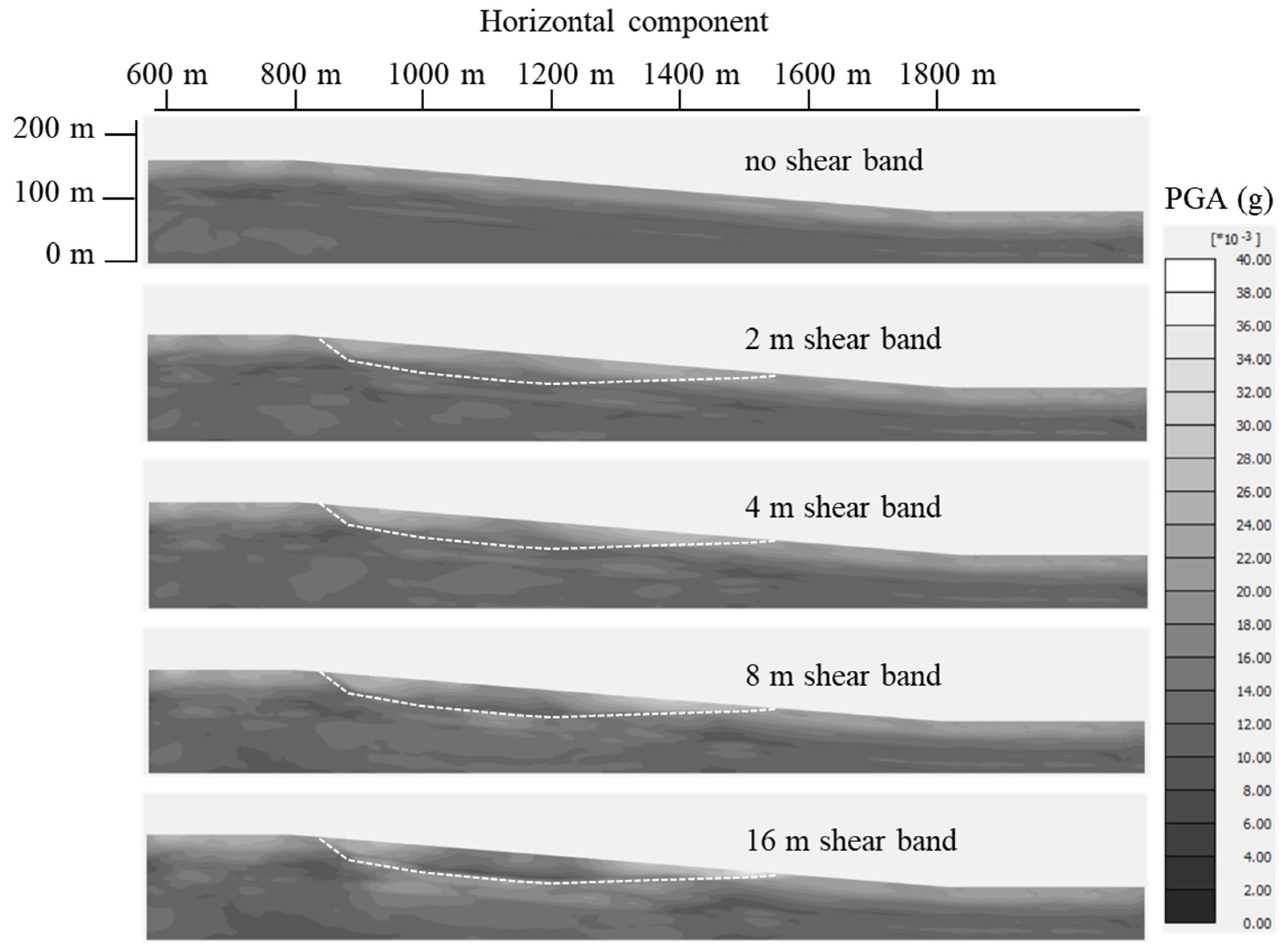
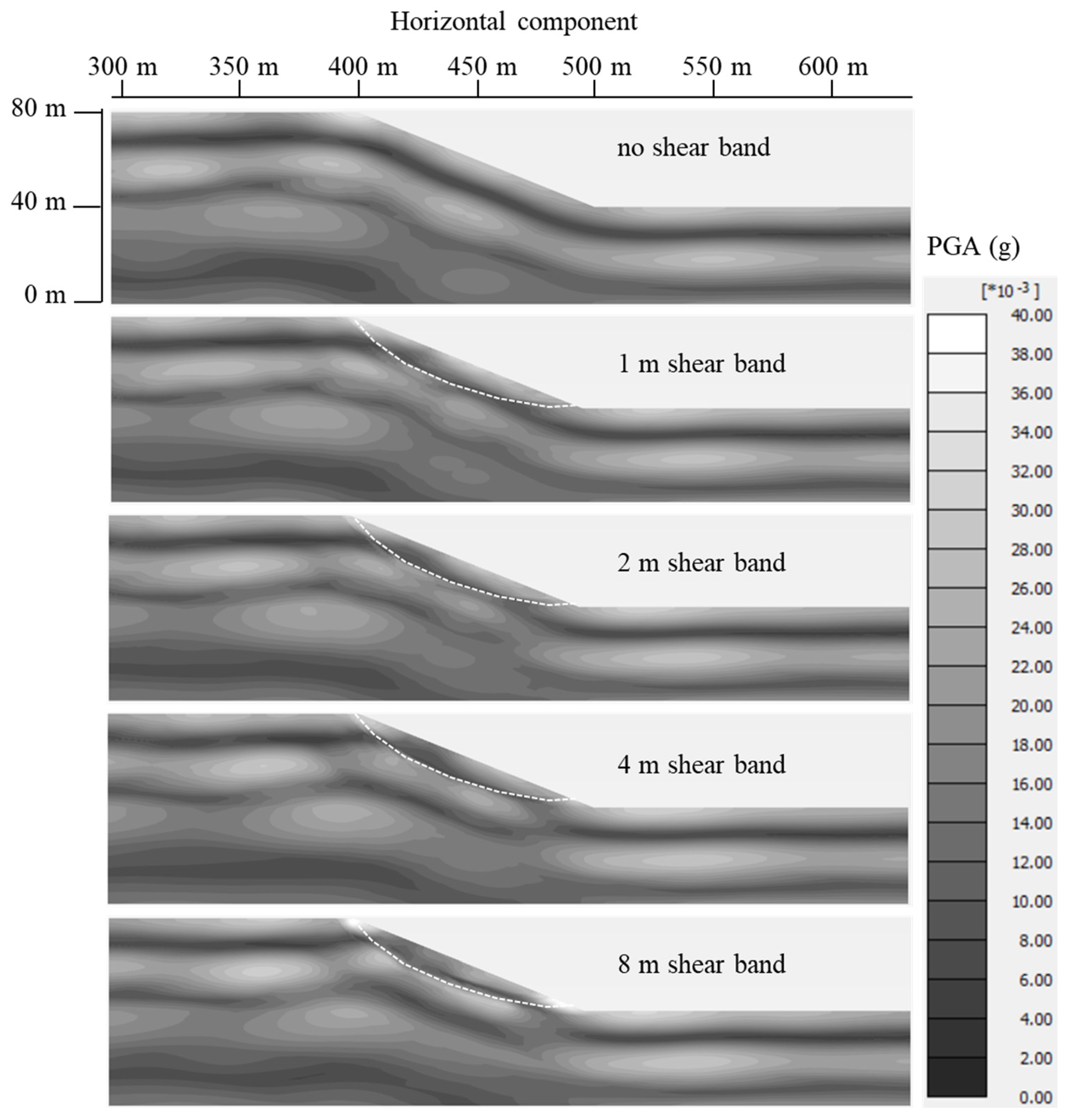
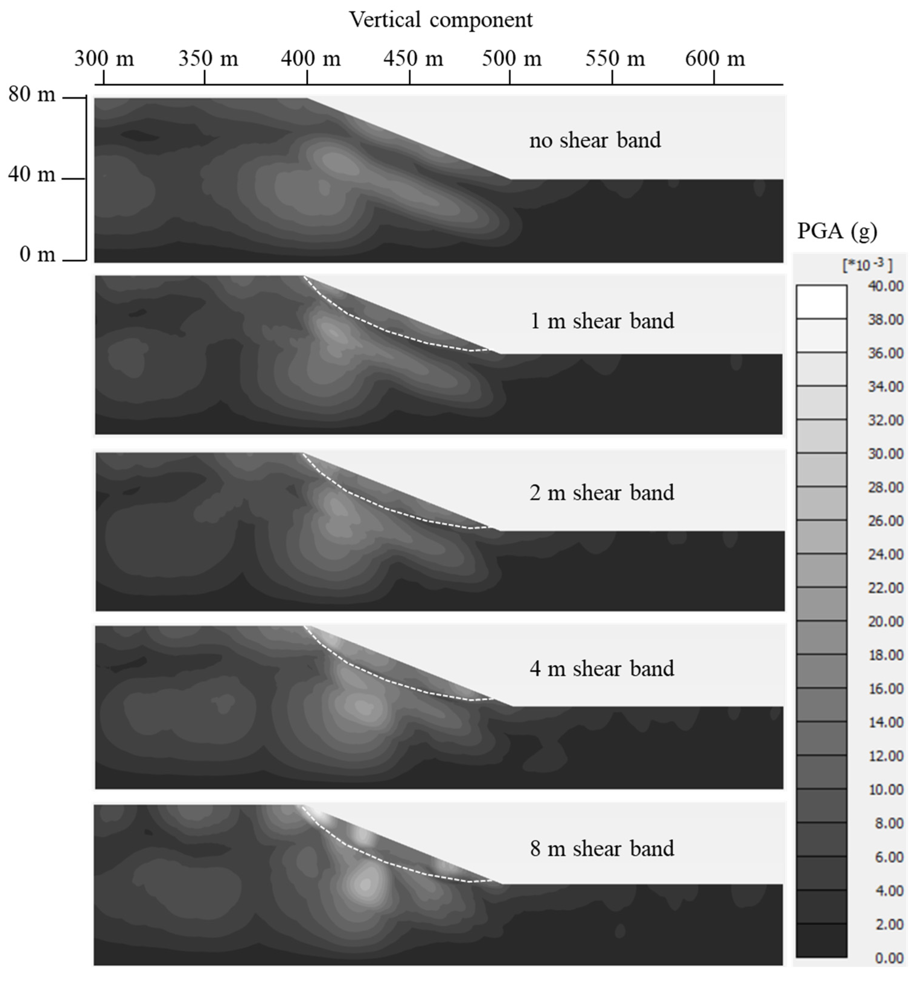
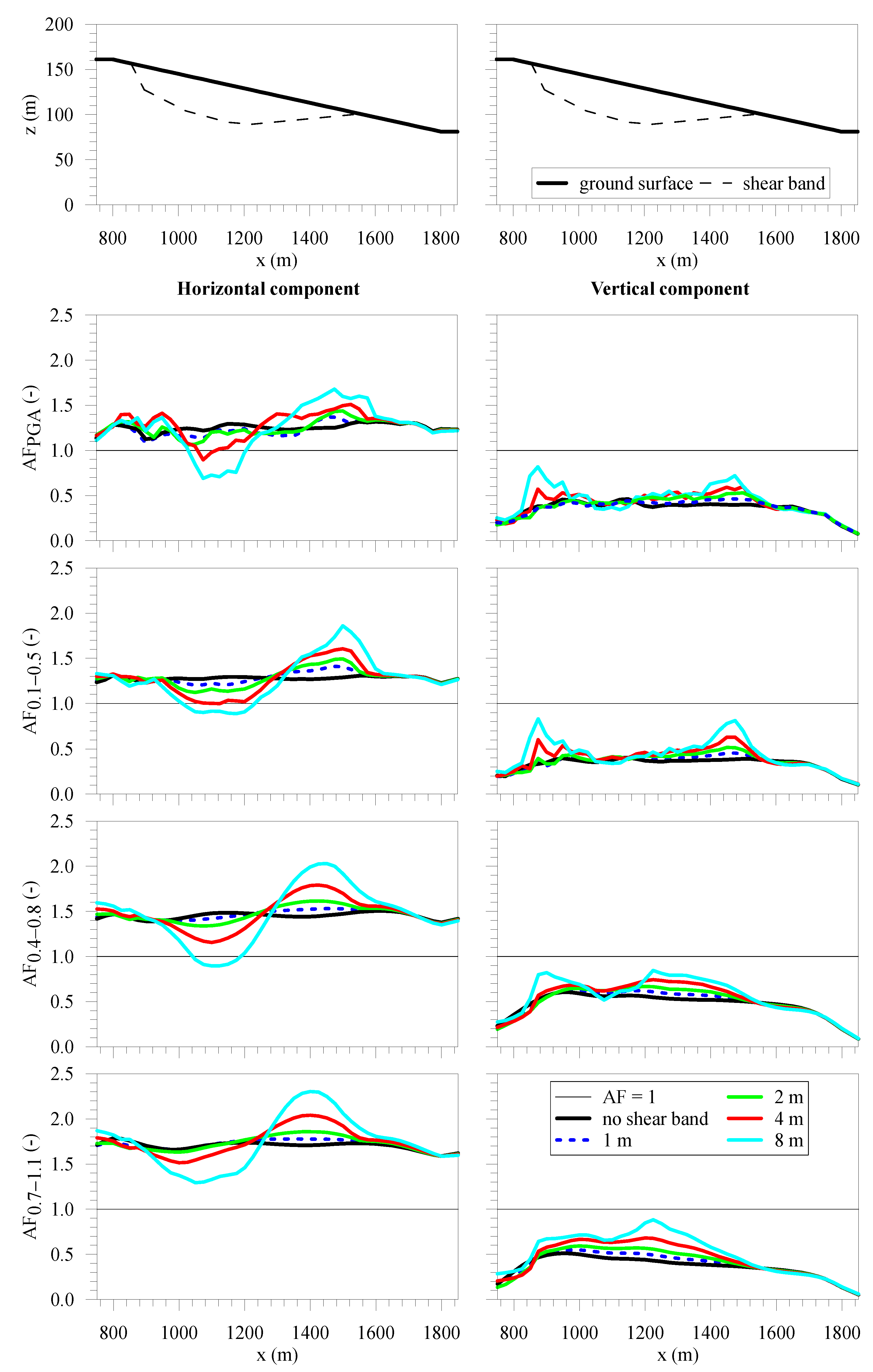
3. Interpretation of the Numerical Results

The results of the 2D simulations are firstly illustrated in terms of the contours of the maximum values of PGA attained by the horizontal and vertical motion during the earthquake. As already recalled, a parasitic vertical component of the seismic motion might be generated into slopes due to the wave reflection from the inclined topographic surface and/or at the shear band. Figure 5 and Figure 6 show the contours of the horizontal and vertical PGA values for the Case I models, including or not including the shear bands. With reference to the intact soil case (i.e., no shear band), the PGA contours of the horizontal component (Figure 5) are approximately parallel to the ground surface in the central zone of the slope, thus indicating a prevalent 1D behaviour expected due to the correlation between the predominant wavelength of the input motion and the geometry of the model. Instead, the presence of the shear band clearly affects the distribution of the PGA at the ground surface and inside the entire slope. Indeed, high values of the PGA might be detected at depth for the higher thickness of the weakened material; additionally, the highest PGA values are located close to the crest and beyond the toe downslope for increasing the thickness of the shear band. Figure 6 gives evidence of the existence of a significant component of the vertical motion (maximum value of 0.012 g), already in the case without a shear band, due to the inclined surface of the slope. This parasitic vertical component may become significantly high in the presence of a shear band due to the wave reflections at the contact between the soft soil and the weakened material. In particular, the higher the shear band thickness, the higher the PGA values, which concentrate at the crest of the slope. For example, for the 16 m thick shear band, a maximum PGA of 0.300 g is observed at 850 m, where the shear band outcrops.
The PGA contours of the horizontal and vertical acceleration components obtained for the steep slope (Case II) are presented in Figure 7 and Figure 8, respectively. As for the gentle slope, the thicker the shear band, the higher the PGA values recorded within the FE model. However, for the steep slope cases, it is more evident how the PGA distribution in the upslope and downslope areas (i.e., above the crest and beyond the toe) depends on the coupling between the shear band and topography effects. In particular, the amplification of the vertical motion appears to propagate above the crest with the increasing thickness of the weakened band (see x = 350 m in Figure 8).
The 2D results are then interpreted in terms of amplification factors at the surface, which provide the quantification of ground motion modification with reference to different period intervals and allow us to display the site effects in an easy-to-read fashion within a seismic hazard perspective (e.g., [58,79,80,81]). The amplification factors are defined as the ratio between a quantity describing the seismic motion recorded at the ground surface and the same quantity describing the input motion:
AF PGA = PGA o PGA i
AF T 1 T 2 = T 1 T 2 Sa o dT T 1 T 2 Sa i dT
where Sa is the pseudo-spectral acceleration, and T is the period. The subscripts “i” and “o” refer, respectively, to the input and output motions, the latter recorded at the ground surface. The AFT1–T2 are evaluated as the ratio of the integral of the pseudo-acceleration response spectra (5% structural damping) over predefined period ranges, T1–T2. Specifically, the period intervals adopted in this study are 0.1–0.5, 0.4–0.8 and 0.7–1.1 s.
The profiles along the slope ground surface of the amplification factors (AF) are shown in Figure 9 for Case I. The AFs relative to the vertical component of the surface motion (presented on the right side of the figure) have been calculated with respect to the horizontal component of the input motion. As expected, the profiles of the amplification factors in the shear band area (highlighted in the upper part of the figure) are strongly influenced by its presence. Indeed, depending on the period range, the weakened shear bands may be responsible for the amplification of the input motion in some locations but also for its de-amplification in other parts of the slope. In particular, the higher the thickness of the weakened zone, the higher the maximum absolute value of the amplification factors in the shear band area. For example, for the 16 m thick shear band slope model, the AFPGA profile of the horizontal component of the motion is characterised by a minimum of 0.7 and a maximum of 1.6; the AF0.1–0.5 profile shows a minimum value of 0.9 and a maximum of 1.7, while in the long period range of 0.7–1.1 s, the AF0.7–1.1 profile gives evidence for the amplification of the motion along the entire slope surface. Additionally, it might be observed that the AFs profiles for the cases with the shear band are characterised by fluctuations around the profile obtained for the intact soil case, showing minimum values in the upper portion of the slope and maximum values in the lower portion of the slope. The location of the maximum values of the horizontal and vertical AFs tend to move toward the toe of the slope for increasing thickness of the weakened zone. Conversely, only the amplification factor of the horizontal motion in terms of PGA considerably increases at the crest with respect to the case of intact soil. Additionally, it might be remarked that, for all the examined cases, the parasitic vertical component is always lower than the horizontal component of the input motion (i.e., AFs less than 1). The highest amplification of the vertical component is observed in the 0.7–1.1 s interval of the period for the thickest shear band case.
Figure 10 presents the profiles of the AFs for Case II. The amplification factors calculated for both the horizontal and vertical components in the mid and higher period ranges are slightly affected by the presence of the weakened zone in the FE model. Instead, the AFs in terms of PGA and in the lower period range (i.e., 0.1–0.5 s) are considerably altered by the shear band, showing numerous oscillations between the minimum and maximum values. Peaks of the amplification factor profiles are detected in different locations of the slope surface, with the maximum around the toe of the slope. Additionally, in this case, the presence of the weakened zone may generate a de-amplification of the horizontal component of the motion, which is more significant the thicker the shear band is. Moreover, the parasitic vertical component induced by the topography and the morphology of the shear band is significantly higher in the low period range and considerably amplified for the increased thickness of the shear band: for thicker shear bands, i.e., 4 m and 8 m, the vertical component could be even higher than the horizontal component of the input motion (see the right side of Figure 10).
Table 3 shows the amplification factors (Afs) at control point locations xr = 0.2, 0.5 and 0.8 for both Cases I and II, considering or not considering the presence of the shear bands. It should be noted that the amplitudes of the AFs over different period ranges are strongly dependent on both the shear band thickness and the position of the point of interest.
Figure 11 and Figure 12 show the plots of the horizontal and vertical components of the surface motions recorded at three control nodes on the ground surface for Case I and Case II, respectively. The relative normalised distance of the nodes (i.e., xr) is shown in the figures. It might be noted that, for the intact soil slope (i.e., figures entitled “no s.b.”), the directivity of the surface motion is in accordance with the slope inclination, both for Case I and Case II. The presence of the weakened zone causes an increase in the earthquake’s vertical components, while the horizontal ones tend to reduce. This is more evident for the accelerations recorded at the ground surface of the Case I model at xr = 0.2 and 0.5 when the thickness of the shear band is 8 m and 16 m (Figure 11) and at the ground surface of the Case II model at xr = 0.2 and 0.5 for a shear band thickness of 4 m and 8 m (Figure 12). Moreover, the acceleration seems to be orthogonal to the ground surface in Case II at xr = 0.2 for a shear band thickness of 8 m, thus showing a prevailing effect on the ground motion modification of the weak zone presence on the topographic effect. Therefore, the ground motion polarisation in the vertical plane is somehow influenced by the presence of a thick shear band, thus confirming what has been observed, for example, by Del Gaudio and co-workers [52,54,55], through HVSR measurements on quiescent landslide bodies. Nevertheless, the 2D numerical simulations performed in this work do not allow us to estimate the polarisation of the motion induced in the horizontal plane by the landslide body (e.g., [41,82]). This effect could only be captured through a comprehensive study based on 3D numerical simulations [83], which is out of the scope of the paper.
The percentage difference between the AFs calculated for slope models with and without shear band can be quantified through the following expression:
Δ AF = AF with   shear   band AF without   shear   band AF without   shear   band 100
Figure 13 and Figure 14 illustrate the ΔAF profiles relative to Case I and II, respectively. For Case I, the ΔAF referring to the horizontal component are in the range ±40%, while the percentage differences in the AFs of the vertical motion are much higher, especially above the crest and at the toe of the slope, reaching a maximum value of about 150% in the case of the ΔAF calculated in the period range 0.1–0.5 s. Considering Case II, the presence of the shear band affects the amplification factors calculated in the low period ranges and the ΔAF referring to the PGA of the vertical component attains its maximum of 200% at the crest of the slope when a weakened zone of 8 m is considered. In general, the effect of the pre-existing shear band seems to be more pronounced on the vertical motion rather than on the horizontal one.
With the purpose of separating and distinguishing the geometric effects (i.e., ground motion modifications induced by the uneven topography and by the buried morphology) from the stratigraphic effects, the latter related to the presence of different soft materials in the subsoil, additional 1D FE seismic analyses were performed with reference to 1D soil columns characterised by the same soil stratigraphy and depth as that extracted from the 2D FE models along the vertical passing through the observation points at xr = 0.2. Figure 15 shows the surface response spectra of the horizontal accelerations obtained at xr = 0.2 by means of 1D and 2D numerical schemes for Case I, while Figure 16 presents the same comparison for Case II. The 2D results are different from those obtained with the 1D models, with higher spectral accelerations predicted by the 1D scheme in almost all the investigated cases. Greater differences are observed for the gentle slope case with respect to the steep slope case. The comparison between 2D and 1D response spectra in the case without a shear band gives evidence to solely the topographic effects. The discrepancies between 1D and 2D response spectra predicted by the models, including the shear bands, are, instead, related not only to the sloping topography but also to the morphology of the weakened area. This confirms that the site response at the surface is affected by both the geometrical shape and thickness of the weakened zone. Moreover, it is worth noting that 1D models cannot predict the vertical motion induced by the geometric effect, which is related to topography and buried morphology, while the 1D horizontal ground motion seems to be consistent with the 2D horizontal response.
Finally, the numerical results are illustrated in terms of amplification functions determined as the ratio of the Fourier spectra obtained at the ground surface and at the interface between the soft soil and the bedrock. The amplification functions, shown in Figure 17, are referred to as the control points at xr = 0.2, 0.5 and 0.8 for the two analysed case studies.
With reference to Case I, it might be observed that the fundamental frequency, f0, is not particularly affected by the presence of the shear band, attaining a value of about 1 Hz independently of the shear band thickness, while all the other natural frequencies reduce for the increased thickness of the band, apart from xr = 0.8 (i.e., near the toe). The f0 for 1D and 2D models can be evaluated through Equations (4) and (5), respectively, according to [1,84]:
f 0 _ 1 D = V S 4 H
f 0 _ 2 D = V S 5 H
where H is the thickness and VS is the shear wave velocity of the soft soil layer. Hence, considering VS = 400 m/s and H = 80 m for Case I, f0_1D and f0_2D are equal to 1.00 Hz and 1.25 Hz, respectively. The f0 values obtained by means of the numerical simulations range between 1.00 and 1.25 Hz. In particular, the second and the third natural frequencies reduce to about 40% when considering the 16 m thick shear band with respect to the case of intact soil (i.e., no shear band) for xr = 0.2 and 0.5. A similar pattern might be recognised for Case II simulations. Indeed, for the three selected nodes on the ground surface, the fundamental frequency f0 remains in the range of 2.00–2.50 Hz, while the higher natural frequencies seem to undergo a reduction dependent on the shear band thickness. In this case, the second natural frequency, equal to 8.5 Hz in the absence of the shear band, decreases to 6.5 Hz at xr = 0.2 when the weakened zone is 8 m thick. The other natural frequencies at xr = 0.5 and 0.8 are, instead, not easy to detect. Furthermore, the amplification peak amplitude Af0 corresponding to the fundamental frequency f0 is strongly dependent on the thickness of the weakened zone (e.g., [83,85]). As an example, a significant reduction from a value of 10 in the case of the intact soil to about 7 for the thickest shear band was recognised at xr = 0.5 in Case I, while at xr = 0.8, the Af0 was about 10 disregarding the presence of the shear band.
The profiles of Af0 along the slope surface are depicted in Figure 18, revealing the complex correlation between the thickness of the shear band and the amplification response. For Case I, the Af0 profiles for the higher thicknesses of the weakened zone (i.e., 8 and 16 m) are much lower than those achieved with the thinner bands, indicating a damping effect on the fundamental frequency, which increases with the thickness of the weakened zone. Shear bands of 2 m and 4 m thickness generate higher Af0 in the middle–top part of the slope (between 800 m and 1300 m) with respect to the case of no shear band. Additionally, in Case II, a more pronounced amplification of the first natural frequency can be observed near and beyond the crest area when weakened zones of 1 and 2 m are included in the numerical model, while the 8 m thick shear band causes a peak in the Af0 profile just above the crest.
Referring to slopes without a pre-existing shear band or, in general, without a quiescent landslide body, other researchers (e.g., [83,84,86,87]) have proved that the profiles of Af0 from numerical analysis are in satisfactory agreement with the Af0 profiles obtained through ambient noise measurements (e.g., HVSR). On the other hand, no example of Af0 profiles for slopes with a pre-existing shear band has been provided by other authors who, instead, have focused their attention on the directivity effect on the HVSR measurement induced by a buried morphology [52,54,55,82,88]. Furthermore, Figure 18 shows that the Af0 profiles are correlated to the slope inclination and to the presence of a shear band. In detail, the Af0 profiles are correlated to the thickness of the shear band. Moreover, for a fixed thickness of the weakened zone and a fixed slope inclination, different geometries of the shear band are expected to provide different Af0 profiles. In this context, bearing in mind that rapid population growth often forces the urbanisation of quiescent or unstable areas, the comparison between ambient noise measurements (e.g., HVSR) and preliminary slope modelling results (such as those presented in Figure 18) could support and guide the design of site-specific investigations with depth, aimed at better constraining the buried morphology of the landslide body (e.g., [82,88,89,90]). The following working flow could be considered in these cases:
(1)
geomorphological analysis of the area of interest;
(2)
collection of soil data (physical and mechanical properties) from available archives;
(3)
definition of a preliminary site model including the buried morphology (i.e., shape and thickness of the shear band);
(4)
ambient noise measurements aimed at providing Af0 profiles;
(5)
performing a parametric analysis by means of numerical simulations based on the preliminary site model and varying the shape and the thickness of the shear band;
(6)
comparison between numerical results and site data in terms of Af0 profiles;
(7)
selection of the most suitable site model which gives comparable results with site data;
(8)
design and execution of site-specific investigations (e.g., continuous coring borehole, inclinometers, etc.) in order to verify the site model selected at the previous point;
(9)
release of the definitive subsoil geotechnical model.

4. Conclusions

This paper presents some preliminary results on the influence of pre-existing shear bands, confining a landslide body, on the seismic wave propagation processes of two step-like ideal slopes subjected to weak earthquakes, performed through a 2D finite element approach. Two ground surface configurations, representing gentle and steep natural slopes, were analysed, whose geometry was appropriately selected to consider the occurrence of negligible and high topographic amplification effects. The pre-existing shear bands were implemented in the numerical models as weakened zones of reduced mechanical properties with respect to the surrounding soil, characterised by different thicknesses. Since the plasticity-induced effects are beyond the scope of the paper, the bedrock input motions were scaled to a very low peak acceleration, while the slope soils were modelled as a linear visco-elastic material.
The results of the numerical simulations indicate that the presence of a pre-existing shear band may significantly affect the dynamic response inside the slope and at the ground surface. In the case of a gentle natural slope (i.e., Case I), for which negligible topographic amplification was expected, a higher thickness of the weakened zone and higher peak values of the amplification factors were recorded. For steep slopes (i.e., Case II, for which high topographic effects are predictable), instead, only the AFs calculated in terms of PGA and in the lower period range are influenced by the presence of the shear band. In particular, for gentle slopes affected by a landslide body confined by a thick shear band, the highest amplification factors are expected in the longer period range of 0.7–1.1 s, while the highest level of amplification is achieved in the intermediate period interval of 0.4–0.8 s in the case of steep slopes. Moreover, the parasitic vertical component may be pronounced, especially in the case of steep topography, for which the effects of the shear band morphology enhance those related to the topographic profile. Indeed, the presence of a thick shear band may force the polarization of the ground motion in the direction normal to the slope surface. Finally, it is shown that the fundamental frequency of the deposit is not particularly affected by the presence of the shear band along the slope for the analysed case studies, while the amplitude of the amplification function at the fundamental frequency is clearly related to the thickness of the shear band. As a matter of fact, more complex shear band geometries or thicker weakened zones are expected to modify also the f0 values with respect to the case of the intact soil (i.e., without the shear band).
The numerical study highlights the importance of considering the actual position, shape and thickness of a pre-existing shear band in the site response analysis of natural slopes performed from a seismic risk mitigation perspective (e.g., microzonation studies). Therefore, the subsoil geotechnical model should be based on detailed site investigations aimed at identifying and geometrically locating the possible weakened zone, even if the slope area of interest is characterised by a non-active sliding mechanism. Conversely, bearing in mind that site investigations in unstable areas are generally expensive, the numerical results of seismic site response based on preliminary slope modelling could be compared to ambient noise measurements in order to support the design of invasive investigations with depth tailored at better constraining the buried morphologies of the body of the landslide.

Author Contributions

Conceptualisation, G.F. and G.E.; methodology, G.F. and G.E.; validation, G.F. and A.d.L.; formal analysis, G.F.; data curation, G.F. and A.d.L.; writing—original draft preparation, G.F., G.E. and A.d.L..; writing—review and editing, G.F., G.E. and A.d.L.; visualisation, G.F., G.E. and A.d.L.; supervision, G.F., G.E. and A.d.L.; project administration, G.E.; funding acquisition, G.E. All authors have read and agreed to the published version of the manuscript.

Funding

The research has been supported by the PON-MITIGO project (ARS01_00964). The second author is grateful for the financial support received by the project “National Centre for HPC, Big Data and Quantum Computing—Spoke 5: Environment and Natural Disasters” (CN_00000013) funded by the National Recovery and Resilience Plan (NRRP), M4_C2_1.4—NextGenerationEU.

Data Availability Statement

The data presented in this study are available on request from the corresponding author.

Acknowledgments

The Authors would like to thank the anonymous Reviewers for their valuable comments that allowed to improve the quality of the paper.

Conflicts of Interest

The authors declare no conflict of interest.

References

  1. Kramer, S. Geotechnical Earthquake Engineering; Prentice Hall: Upper Saddle River, NJ, USA, 1996; ISBN 9780133749434. [Google Scholar]
  2. Gazetas, G. Vibrational characteristics of soil deposits with variable wave velocity. Int. J. Numer. Anal. Methods Geomech. 1982, 6, 1–20. [Google Scholar] [CrossRef]
  3. Gelagoti, F.; Kourkoulis, R.; Anastasopoulos, I.; Tazoh, T.; Gazetas, G. Seismic Wave Propagation in a Very Soft Alluvial Valley: Sensitivity to Ground-Motion Details and Soil Nonlinearity, and Generation of a Parasitic Vertical Component. Bull. Seismol. Soc. Am. 2010, 100, 3035–3054. [Google Scholar] [CrossRef]
  4. Ciancimino, A.; Lanzo, G.; Alleanza, G.A.; Amoroso, S.; Bardotti, R.; Biondi, G.; Cascone, E.; Castelli, F.; Giulio, A.D.; d’Onofrio, A.; et al. Dynamic characterization of fine-grained soils in Central Italy by laboratory testing. Bull. Earthq. Eng. 2019, 18, 5503–5531. [Google Scholar] [CrossRef]
  5. D’Oria, A.F.; Elia, G.; di Lernia, A.; Uva, G. Influence of soil deposit heterogeneity on the dynamic behaviour of masonry towers. In Proceedings of the 3rd International Symposium on Geotechnical Engineering for the Preservation of Momenuments and Historic Sites (TC301–IS Napoli 2022), Naples, Italy, 22–24 June 2022. [Google Scholar]
  6. Assimaki, D.; Gazetas, G.; Kausel, E. Effects of Local Soil Conditions on the Topographic Aggravation of Seismic Motion: Parametric Investigation and Recorded Field Evidence from the 1999 Athens Earthquake. Bull. Seismol. Soc. Am. 2005, 95, 1059–1089. [Google Scholar] [CrossRef]
  7. Gazetas, G.; Kallou, P.V.; Psarropoulos, P.N. Topography and Soil Effects in the MS 5.9 Parnitha (Athens) Earthquake: The Case of Adámes. Nat. Hazards 2002, 27, 133–169. [Google Scholar] [CrossRef]
  8. Elia, G.; di Lernia, A.; Rouainia, M. Ground motion scaling for the assessment of the seismic response of a diaphragm wall. In Proceedings of the 7ICEGE. VII International Conference on Earthquake Geotechnical Engineering, Rome, Italy, 17–20 June 2019; pp. 2249–2257. [Google Scholar]
  9. Rathje, E.M.; Kottke, A.R.; Trent, W.L. Influence of Input Motion and Site Property Variabilities on Seismic Site Response Analysis. J. Geotech. Geoenviron. Eng. 2010, 136, 607–619. [Google Scholar] [CrossRef]
  10. Guzel, Y.; Elia, G.; Rouainia, M.; Falcone, G. The Influence of Input Motion Scaling Strategies on Nonlinear Ground Response Analyses of Soft Soil Deposits. Geoscience 2023, 13, 17. [Google Scholar] [CrossRef]
  11. Pagliaroli, A.; Lanzo, G.; D’Elia, B. Numerical Evaluation of Topographic Effects at the Nicastro Ridge in Southern Italy. J. Earthq. Eng. 2011, 15, 404–432. [Google Scholar] [CrossRef]
  12. Gobbi, S.; Lenti, L.; Santisi d’Avila, M.P.; Semblat, J.F.; Reiffsteck, P. Influence of the variability of soil profile properties on weak and strong seismic response. Soil Dyn. Earthq. Eng. 2020, 135, 106200. [Google Scholar] [CrossRef]
  13. Guzel, Y.; Rouainia, M.; Elia, G. Effect of soil variability on nonlinear site response predictions: Application to the Lotung site. Comput. Geotech. 2020, 121, 103444. [Google Scholar] [CrossRef]
  14. Falcone, G.; Acunzo, G.; Mendicelli, A.; Mori, F.; Naso, G.; Peronace, E.; Porchia, A.; Romagnoli, G.; Tarquini, E.; Moscatelli, M. Seismic amplification maps of Italy based on site-specific microzonation dataset and one-dimensional numerical approach. Eng. Geol. 2021, 289, 106170. [Google Scholar] [CrossRef]
  15. De Risi, R.; Penna, A.; Simonelli, A.L. Seismic risk at urban scale: The role of site response analysis. Soil Dyn. Earthq. Eng. 2019, 123, 320–336. [Google Scholar] [CrossRef]
  16. Ciancimino, A.; Foti, S.; Lanzo, G. Stochastic analysis of seismic ground response for site classification methods verification. Soil Dyn. Earthq. Eng. 2018, 111, 169–183. [Google Scholar] [CrossRef]
  17. Tönük, G.; Ansal, A.; Kurtuluş, A.; Çetiner, B. Site specific response analysis for performance based design earthquake characteristics. Bull. Earthq. Eng. 2014, 12, 1091–1105. [Google Scholar] [CrossRef]
  18. Geli, L.; Bard, P.Y.; Jullien, B. The effect of topography on earthquake ground motion: A review and new results. Bull. Seismol. Soc. Am. 1988, 78, 42–63. [Google Scholar] [CrossRef]
  19. Bouckovalas, G.D.; Papadimitriou, A.G. Numerical evaluation of slope topography effects on seismic ground motion. Soil Dyn. Earthq. Eng. 2005, 25, 547–558. [Google Scholar] [CrossRef]
  20. Rizzitano, S.; Cascone, E.; Biondi, G. Coupling of topographic and stratigraphic effects on seismic response of slopes through 2D linear and equivalent linear analyses. Soil Dyn. Earthq. Eng. 2014, 67, 66–84. [Google Scholar] [CrossRef]
  21. Falcone, G.; Boldini, D.; Amorosi, A. Site response analysis of an urban area: A multi-dimensional and non-linear approach. Soil Dyn. Earthq. Eng. 2018, 109, 33–45. [Google Scholar] [CrossRef]
  22. Gatmiri, B.; Arson, C. Seismic site effects by an optimized 2D BE/FE method II. Quantification of site effects in two-dimensional sedimentary valleys. Soil Dyn. Earthq. Eng. 2008, 28, 646–661. [Google Scholar] [CrossRef]
  23. Falcone, G.; Boldini, D.; Martelli, L.; Amorosi, A. Quantifying local seismic amplification from regional charts and site specific numerical analyses: A case study. Bull. Earthq. Eng. 2020, 18, 77–107. [Google Scholar] [CrossRef]
  24. Costanzo, A.; D’Onofrio, A.; Silvestri, F. Seismic response of a geological, historical and architectural site: The Gerace cliff (southern Italy). Bull. Eng. Geol. Environ. 2019, 78, 5617–5633. [Google Scholar] [CrossRef]
  25. di Lernia, A.; Buono, C.; Elia, G. Evaluation of seismic site effects in a real slope through 2D FE numerical analyses. In Proceedings of the 9th ECCOMAS Thematic Conference on Computational Methods in Structural Dynamics and Earthquake Engineering–COMPDYN2023, Athens, Greece, 12–14 June 2023. [Google Scholar]
  26. Moczo, P.; Kristek, J.; Bard, P.Y.; Stripajová, S.; Hollender, F.; Chovanová, Z.; Kristeková, M.; Sicilia, D. Key structural parameters affecting earthquake ground motion in 2D and 3D sedimentary structures. Bull. Earthq. Eng. 2018, 16, 2421–2450. [Google Scholar] [CrossRef]
  27. Zhang, Z.; Fleurisson, J.-A.; Pellet, F. The effects of slope topography on acceleration amplification and interaction between slope topography and seismic input motion. Soil Dyn. Earthq. Eng. 2018, 113, 420–431. [Google Scholar] [CrossRef]
  28. Zhu, C.; Riga, E.; Pitilakis, K.; Zhang, J.; Thambiratnam, D. Seismic Aggravation in Shallow Basins in Addition to One-dimensional Site Amplification. J. Earthq. Eng. 2020, 24, 1477–1499. [Google Scholar] [CrossRef]
  29. Zhu, C.; Thambiratnam, D.; Gallage, C. Inherent Characteristics of 2D Alluvial Formations Subjected to In-Plane Motion. J. Earthq. Eng. 2019, 23, 1512–1530. [Google Scholar] [CrossRef]
  30. Tripe, R.; Kontoe, S.; Wong, T.K.C. Slope topography effects on ground motion in the presence of deep soil layers. Soil Dyn. Earthq. Eng. 2013, 50, 72–84. [Google Scholar] [CrossRef]
  31. Kwok, A.O.L.; Stewart, J.P.; Hashash, Y.M.A.; Matasovic, N.; Pyke, R.; Wang, Z.; Yang, Z. Use of exact solutions of wave propagation problems to guide implementation of nonlinear seismic ground response analysis procedures. J. Geotech. Geoenviron. Eng. 2007, 133, 1385–1398. [Google Scholar] [CrossRef]
  32. Schnabel, P.B.; Lysmer, J.; Seed, H.B. SHAKE: A Computer Program for Earthquake Response Analysis of Horizontally Layerd Sites; Report EERC 72-12; Earthquake Engineering Research Center, University of California: Berkley, CA, USA, 1972. [Google Scholar]
  33. Idriss, I.M.; Lysmer, J.; Hwang, R.; Seed, H.B. QUAD-4: A Computer Program for Evaluating the Seismic Response of Soil Structures by Variable Damping Finite Element Procedures; Report no EERC 73-16; Earthquake Engineering Research Center, University of California: Berkley, CA, USA, 1973. [Google Scholar]
  34. Amorosi, A.; Boldini, D.; Elia, G. Parametric study on seismic ground response by finite element modelling. Comput. Geotech. 2010, 37, 515–528. [Google Scholar] [CrossRef]
  35. Régnier, J.; Bonilla, L.; Bard, P.; Bertrand, E.; Hollender, F.; Kawase, H.; Sicilia, D.; Arduino, P.; Amorosi, A.; Asimaki, D.; et al. International Benchmark on Numerical Simulations for 1D, Nonlinear Site Response (PRENOLIN): Verification Phase Based on Canonical Cases. Bull. Seismol. Soc. Am. 2016, 106, 2112–2135. [Google Scholar] [CrossRef]
  36. Régnier, J.; Bonilla, L.; Bard, P.; Bertrand, E.; Hollender, F.; Kawase, H.; Sicilia, D.; Arduino, P.; Amorosi, A.; Asimaki, D.; et al. PRENOLIN: International Benchmark on 1D Nonlinear Site-Response Analysis—Validation Phase Exercise. Bull. Seismol. Soc. Am. 2018, 108, 876–900. [Google Scholar] [CrossRef]
  37. Tropeano, G.; Soccodato, F.M.; Silvestri, F. Re-evaluation of code-specified stratigraphic amplification factors based on Italian experimental records and numerical seismic response analyses. Soil Dyn. Earthq. Eng. 2018, 110, 262–275. [Google Scholar] [CrossRef]
  38. di Lernia, A.; Amorosi, A.; Boldini, D. A multi-directional numerical approach for the seismic ground response and dynamic soil-structure interaction analyses. In Proceedings of the 7ICEGE. VII International Conference on Earthquake Geotechnical Engineering, Roma, Italy, 17–20 June 2019; pp. 2145–2152. [Google Scholar]
  39. Newmark, N.M. Effects of Earthquakes on Dams and Embankments. Géotechnique 1965, 15, 139–160. [Google Scholar] [CrossRef]
  40. Jibson, R.W. Methods for assessing the stability of slopes during earthquakes—A retrospective. Eng. Geol. 2011, 122, 43–50. [Google Scholar] [CrossRef]
  41. Del Gaudio, V.; Wasowski, J. Advances and problems in understanding the seismic response of potentially unstable slopes. Eng. Geol. 2011, 122, 73–83. [Google Scholar] [CrossRef]
  42. Lenti, L.; Martino, S. The interaction of seismic waves with step-like slopes and its influence on landslide movements. Eng. Geol. 2012, 126, 19–36. [Google Scholar] [CrossRef]
  43. Lenti, L.; Martino, S. A parametric numerical study of the interaction between seismic waves and landslides for the evaluation of the susceptibility to seismically induced displacements. Bull. Seismol. Soc. Am. 2013, 103, 33–56. [Google Scholar] [CrossRef]
  44. Ren, Z.; Chen, C.; Sun, C.; Wang, Y. Dynamic Analysis of the Seismo-Dynamic Response of Anti-Dip Bedding Rock Slopes Using a Three-Dimensional Discrete-Element Method. Appl. Sci. 2022, 12, 4640. [Google Scholar] [CrossRef]
  45. Rollo, F.; Rampello, S. Probabilistic assessment of seismic-induced slope displacements: An application in Italy. Bull. Earthq. Eng. 2021, 19, 4261–4288. [Google Scholar] [CrossRef]
  46. Zhang, L.; Yang, C.; Ma, S.; Guo, X.; Yue, M.; Liu, Y. Seismic Response Time-Frequency Analysis of Bedding Rock Slope. Front. Phys. 2020, 8, 558547. [Google Scholar] [CrossRef]
  47. Leroueil, S. Natural slopes and cuts: Movement and failure mechanisms. Geotechnique 2001, 51, 197–243. [Google Scholar] [CrossRef]
  48. Chandler, R.J.; Willis, M.R.; Hamilton, P.S.; Andreou, I. Tectonic shear zones in the London Clay Formation. Geotechnique 1998, 48, 257–270. [Google Scholar] [CrossRef]
  49. Picarelli, L.; Leroueil, S.; Urciuoli, G.; Guerriero, G.; Delisle, M.C. Occurrence and features of shear zones in clay. In Proceedings of the International Workshop on Localization and Bifurcation Theory for Soils and Rocks, Gifu, Japan, 28 September–2 October 1997; pp. 259–270. [Google Scholar]
  50. Hutchinson, J.N. Methods of locating slip surfaces in landslides. AEG Bull. 1983, 20, 235–252. [Google Scholar] [CrossRef]
  51. Bordoni, P.; Haines, J.; Di Giulio, G.; Milana, G.; Augliera, P.; Cercato, M.; Martelli, L.; Cara, F.; Horleston, A.; Cattaneo, M.; et al. Cavola experiment site: Geophysical investigations and deployment of a dense seismic array on a landslide. Ann. Geophys. 2007, 50, 627–649. [Google Scholar] [CrossRef]
  52. Del Gaudio, V.; Wasowski, J. Directivity of slope dynamic response to seismic shaking. Geophys. Res. Lett. 2007, 34, L12301. [Google Scholar] [CrossRef]
  53. Bozzano, F.; Lenti, L.; Martino, S.; Paciello, A.; Scarascia Mugnozza, G. Self-excitation process due to local seismic amplification responsible for the reactivation of the Salcito landslide (Italy) on 31 October 2002. J. Geophys. Res. 2008, 113, B10312. [Google Scholar] [CrossRef]
  54. Del Gaudio, V.; Coccia, S.; Wasowski, J.; Gallipoli, M.R.; Mucciarelli, M. Detection of directivity in seismic site response from microtremor spectral analysis. Nat. Hazards Earth Syst. Sci. 2008, 8, 751–762. [Google Scholar] [CrossRef]
  55. Del Gaudio, V.; Luo, Y.; Wang, Y.; Wasowski, J. Using ambient noise to characterise seismic slope response: The case of Qiaozhuang peri-urban hillslopes (Sichuan, China). Eng. Geol. 2018, 246, 374–390. [Google Scholar] [CrossRef]
  56. Bouckovalas, G.D.; Papadimitriou, A.G. Aggravation of seismic ground motion due to slope topography. In Proceedings of the 1st European Conference on Earthquake Engineering and Seismology, Geneva, Switzerland, 3–8 September 2006. No. 1171. [Google Scholar]
  57. Moscatelli, M.; Albarello, D.; Scarascia Mugnozza, G.; Dolce, M. The Italian approach to seismic microzonation. Bull. Earthq. Eng. 2020, 18, 5425–5440. [Google Scholar] [CrossRef]
  58. Mori, F.; Gaudiosi, I.; Tarquini, E.; Bramerini, F.; Castenetto, S.; Naso, G.; Spina, D. HSM: A synthetic damage-constrained seismic hazard parameter. Bull. Earthq. Eng. 2020, 18, 5631–5654. [Google Scholar] [CrossRef]
  59. Griffiths, D.V.; Lane, P.A. Slope stability analysis by finite elements. Geotechnique 1999, 49, 387–403. [Google Scholar] [CrossRef]
  60. Henkel, D.J. Discussion. Earth movement affecting L.T.E. railway in deep cutting east of Uxbridge. Proc. Inst. Civ. Eng. Part I 1956, 5, 320–323. [Google Scholar]
  61. Watson, J.D. Earth movement affecting LTE railway in deep cutting east of Uxbridge. Proc. Inst. Civ. Eng. Part II 1956, 5, 302–316. [Google Scholar]
  62. Urciuoli, G.; Pirone, M.; Comegna, L.; Picarelli, L. Long-term investigations on the pore pressure regime in saturated and unsaturated sloping soils. Eng. Geol. 2016, 212, 98–119. [Google Scholar] [CrossRef]
  63. Vassallo, R.; Calcaterra, S.; D’Agostino, N.; De Rosa, J.; Di Maio, C.; Gambino, P. Long-Term Displacement Monitoring of Slow Earthflows by Inclinometers and GPS, and Wide Area Surveillance by COSMO-SkyMed Data. Geosciences 2020, 10, 171. [Google Scholar] [CrossRef]
  64. Comegna, L.; Picarelli, L.; Urciuoli, G. The mechanics of mudslides as a cyclic undrained-drained process. Landslides 2007, 4, 217–232. [Google Scholar] [CrossRef]
  65. di Lernia, A.; Cotecchia, F.; Elia, G.; Tagarelli, V.; Santaloia, F.; Palladino, G. Combined use of hydraulic and coupled hydro-mechanical numerical modelling of the response of a clay slope to climatic actions in the long term. Ital. Geotech. J. 2023, accepted. [Google Scholar]
  66. Cotecchia, F.; Vitone, C.; Petti, R.; Soriano, I.; Santaloia, F.; Lollino, P. Slow landslides in urbanised clayey slopes: An emblematic case from the south of Italy. In Landslides and Engineered Slopes. Experience, Theory and Practice; Taylor and Francis Inc.: Abingdon, UK, 2016; Volume 2, pp. 691–698. ISBN 9781138029880. [Google Scholar]
  67. Lollino, P.; Giordan, D.; Allasia, P.; Fazio, N.L.; Perrotti, M.; Cafaro, F. Assessment of post-failure evolution of a large earthflow through field monitoring and numerical modelling. Landslides 2020, 17, 2013–2026. [Google Scholar] [CrossRef]
  68. Lollino, P.; Cotecchia, F.; Elia, G.; Mitaritonna, G.; Santaloia, F. Interpretation of landslide mechanisms based on numerical modelling: Two case-histories. Eur. J. Environ. Civ. Eng. 2016, 20, 1032–1053. [Google Scholar] [CrossRef]
  69. Bentley PLAXIS 2D CE V20, Reference Manual 2020. Available online: https://www.bentley.com/software/plaxis-2d/ (accessed on 19 April 2022).
  70. Clough, R.W.; Penzien, J. Dynamics of Structures; Computers & Structures, Inc.: Berkley, CA, USA, 1995. [Google Scholar]
  71. Mejia, L.H.; Dawson, E.M. Earthquake deconvolution for FLAC. In Proceedings of the 4th International FLAC Symposium on Numerical Modeling in Geomechanics, Madrid, Spain, 29–31 May 2006; Itasca Consulting Group: Minneapolis, MN, USA, 2006. [Google Scholar]
  72. Bathe, K.J. Finite Element Procedures, 2nd ed.; Prentice Hall: Upper Saddle River, NJ, USA, 1996. [Google Scholar]
  73. Kuhlemeyer, R.L.; Lysmer, J. Finite Element Method Accuracy for Wave Propagation Problems. J. Soil Mech. Found. Div. 1973, 99, 421–427. [Google Scholar] [CrossRef]
  74. Mori, F.; Mendicelli, A.; Moscatelli, M.; Romagnoli, G.; Peronace, E.; Naso, G. A new Vs30 map for Italy based on the seismic microzonation dataset. Eng. Geol. 2020, 275, 105745. [Google Scholar] [CrossRef]
  75. Falcone, G.; Romagnoli, G.; Naso, G.; Mori, F.; Peronace, E.; Moscatelli, M. Effect of bedrock stiffness and thickness on numerical simulation of seismic site response. Italian case studies. Soil Dyn. Earthq. Eng. 2020, 139, 106361. [Google Scholar] [CrossRef]
  76. Romagnoli, G.; Tarquini, E.; Porchia, A.; Catalano, S.; Albarello, D.; Moscatelli, M. Constraints for the Vs profiles from engineering-geological qualitative characterization of shallow subsoil in seismic microzonation studies. Soil Dyn. Earthq. Eng. 2022, 161, 107347. [Google Scholar] [CrossRef]
  77. D’Amico, M.; Felicetta, C.; Russo, E.; Sgobba, S.; Lanzano, G.; Pacor, F.; Luzi, L. Italian Accelerometric Archive v 3.1; Istituto Nazionale di Geofisica e Vulcanologia, Dipartimento della Protezione Civile Nazionale: Rome, Italy, 2020. [CrossRef]
  78. Luzi, L.; Pacor, F.; Puglia, R. Italian Accelerometric Archive v3.0 2019. Available online: https://itaca.mi.ingv.it/ItacaNet_40/#/home (accessed on 19 April 2022).
  79. Lanzo, G.; Silvestri, F.; Costanzo, A.; D’Onofrio, A.; Martelli, L.; Pagliaroli, A.; Sica, S.; Simonelli, A. Site response studies and seismic microzoning in the Middle Aterno valley (L’aquila, Central Italy). Bull. Earthq. Eng. 2011, 9, 1417–1442. [Google Scholar] [CrossRef]
  80. Pagliaroli, A.; Moscatelli, M.; Raspa, G.; Naso, G. Seismic microzonation of the central archaeological area of Rome: Results and uncertainties. Bull. Earthq. Eng. 2014, 12, 1405–1428. [Google Scholar] [CrossRef]
  81. Falcone, G.; Mendicelli, A.; Mori, F.; Fabozzi, S.; Moscatelli, M.; Occhipinti, G.; Peronace, E. A simplified analysis of the total seismic hazard in Italy. Eng. Geol. 2020, 267, 105511. [Google Scholar] [CrossRef]
  82. Del Gaudio, V.; Muscillo, S.; Wasowski, J. What we can learn about slope response to earthquakes from ambient noise analysis: An overview. Eng. Geol. 2014, 182, 182–200. [Google Scholar] [CrossRef]
  83. Diaz-Segura, E.G. Numerical estimation and HVSR measurements of characteristic site period of sloping terrains. Geotech. Lett. 2016, 6, 176–181. [Google Scholar] [CrossRef]
  84. Ashford, S.A.; Sitar, N.; Lysmer, J.; Deng, N. Topographic effects on the seismic response of steep slopes. Bull. Seismol. Soc. Am. 1997, 87, 701–709. [Google Scholar] [CrossRef]
  85. Castellaro, S.; Mulargia, F. The effect of velocity inversions on H/V. Pure Appl. Geophys. 2009, 166, 567–592. [Google Scholar] [CrossRef]
  86. Warnana, D.D.; Soemitro, R.A.A.; Utama, W. Application of Microtremor HVSR Method for Assessing Site Effect in Residual Soil Slope. Int. J. Basic Appl. Sci. IJBAS 2011, 11, 73–78. [Google Scholar]
  87. Wood, C.M.; Cox, B.R. Experimental Data Set of Mining-Induced Seismicity for Studies of Full-Scale Topographic Effects. Earthq. Spectra 2015, 31, 541–564. [Google Scholar] [CrossRef]
  88. Pischiutta, M.; Fondriest, M.; Demurtas, M.; Magnoni, F.; Di Toro, G.; Rovelli, A. Structural control on the directional amplification of seismic noise (Campo Imperatore, central Italy). Earth Planet. Sci. Lett. 2017, 471, 10–18. [Google Scholar] [CrossRef]
  89. Pazzi, V.; Tanteri, L.; Bicocchi, G.; D’Ambrosio, M.; Caselli, A.; Fanti, R. H/V measurements as an effective tool for the reliable detection of landslide slip surfaces: Case studies of Castagnola (La Spezia, Italy) and Roccalbegna (Grosseto, Italy). Phys. Chem. Earth 2017, 98, 136–153. [Google Scholar] [CrossRef]
  90. Setiawan, B.; Jaksa, M.; Griffith, M.; Love, D. Estimating bedrock depth in the case of regolith sites using ambient noise analysis. Eng. Geol. 2018, 243, 145–159. [Google Scholar] [CrossRef]
Figure 1. Geometrical scheme implemented in the FE simulations.
Geosciences 13 00148 g001
Figure 2. Details of the FE model with reference to (a) Case I and (b) Case II. Only the polyline representing the middle of the shear bands is sketched for the sake of simplicity.
Geosciences 13 00148 g002
Figure 3. Reference input motions RM1 and RM2 presented in terms of (a) acceleration time history and (b) pseudo-acceleration response spectrum (5% damping) scaled at the same PGA.
Geosciences 13 00148 g003
Figure 4. Comparison between the examined case studies and the limits of normalised slope height H/λ and slope angle i/90° for which topographic effects become significant [19], with respect to the (a) horizontal and (b) vertical motion.
Geosciences 13 00148 g004
Figure 5. Contours of the PGA of the horizontal component for Case I. The dashed line refers to the polyline in the middle of the shear bands.
Geosciences 13 00148 g005
Figure 6. Contours of the PGA of the vertical component for Case I. The dashed line refers to the polyline in the middle of the shear bands.
Geosciences 13 00148 g006
Figure 7. Contours of the PGA of the horizontal component for Case II. The dashed line refers to the polyline in the middle of the shear bands.
Geosciences 13 00148 g007
Figure 8. Contours of the PGA of the vertical component for Case II. The dashed line refers to the polyline in the middle of the shear bands.
Geosciences 13 00148 g008
Figure 9. Profiles of amplification factors relative to Case I obtained with or without the shear band.
Geosciences 13 00148 g009
Figure 10. Profiles of amplification factors relative to Case II, obtained with or without the shear band.
Geosciences 13 00148 g010
Figure 11. Surface motions recorded in the control nodes at the ground surface for Case I.
Geosciences 13 00148 g011
Figure 12. Surface motions recorded in the control nodes at the ground surface for Case II.
Geosciences 13 00148 g012
Figure 13. Profiles of the percentage difference between the AFs calculated with and without shear band relative to Case I.
Geosciences 13 00148 g013
Figure 14. Profiles of the percentage difference between the AFs calculated with and without shear band relative to Case II.
Geosciences 13 00148 g014
Figure 15. Case I surface response spectra of the horizontal accelerations obtained at xr = 0.2 by means of 1D and 2D numerical models.
Geosciences 13 00148 g015
Figure 16. Case II surface response spectra of the horizontal accelerations obtained at xr = 0.2 by means of 1D and 2D numerical models.
Geosciences 13 00148 g016
Figure 17. Amplification functions referred to xr = 0.2, 0.5, and 0.8 for Case I and Case II.
Geosciences 13 00148 g017
Figure 18. Profiles of the amplification amplitude Af0 at the fundamental frequency f0 for Case I and Case II.
Geosciences 13 00148 g018
Table 1. Properties of the slope soils implemented in the FE simulations.
MaterialSoil Unit Weight
γsoil (kN/m3)
Poisson’s Ratio
ν
Shear Wave Velocity
VS (m/s)
Damping Ratio
D (%)
Soft soil200.254005
Seismic bedrock220.258001
Weakened shear band180.252005
Table 2. Main features of the reference motions selected from the Italian strong motion network.
Station IDDateMwR (km)PGA (g)PGV (m/s)PGD (m)Name
LRS9 September 1998 5.6 18.0 0.165 0.125 0.127 RM1
RQT26 October 2016 5.4 16.7 0.222 0.04947 0.00495 RM2
Table 3. Amplification factors at xr = 0.2, 0.5, and 0.8 for Case I and II with and without a shear band.
Shear Band
Thickness
AFPGAAF0.1–0.5AF0.4–0.8AF0.7–1.1AFPGAAF0.1–0.5AF0.4–0.8AF0.7–1.1AFPGAAF0.1–0.5AF0.4–0.8AF0.7–1.1
(m)(-)(-)(-)(-)(-)(-)(-)(-)(-)(-)(-)(-)
Control point xr0.20.20.20.20.50.50.50.50.80.80.80.8
Case I
-1.241.281.421.661.241.281.451.721.321.301.501.72
21.161.241.401.661.161.321.511.781.331.301.521.74
41.121.171.371.631.191.321.551.831.341.311.541.75
61.241.121.301.511.401.311.601.931.361.321.561.76
81.141.031.181.371.251.201.582.011.381.381.611.81
Case II
-1.111.221.571.301.321.361.401.221.081.251.261.12
11.361.221.611.291.261.311.431.211.081.211.271.11
21.161.201.641.301.151.241.451.211.051.201.291.12
40.931.131.681.311.131.211.521.241.051.171.321.14
80.691.091.781.370.981.211.661.311.301.271.421.21
Disclaimer/Publisher’s Note: The statements, opinions and data contained in all publications are solely those of the individual author(s) and contributor(s) and not of MDPI and/or the editor(s). MDPI and/or the editor(s) disclaim responsibility for any injury to people or property resulting from any ideas, methods, instructions or products referred to in the content.

