Article

Does Microbial and Faunal Pattern Correspond to Dynamics in Hydrogeology and Hydrochemistry? Comparative Study of Two Isolated Groundwater Ecosystems in Münsterland, Germany

by
Sura Abdulghani Alqaragholi
1,*,
Wael Kanoua
2,
Harald Strauss
1 and
Patricia Göbel
1
1
Institute of Geology and Paleontology, University of Münster, 48149 Münster, Germany
2
Department of Petroleum Engineering, Chemical and Petroleum Engineering Faculty, AL Baath University, Homs, Syria
*
Author to whom correspondence should be addressed.
Geosciences 2023, 13(5), 140; https://doi.org/10.3390/geosciences13050140
Submission received: 12 March 2023 / Revised: 19 April 2023 / Accepted: 3 May 2023 / Published: 11 May 2023

Abstract

:
The objective of this study was to assess the temporal and spatial variability of aquatic invertebrates and microbial parameters (biomass and activity) with environmental data in springs, and to determine the impact of key parameters on the ecological situation of a groundwater system. Eight springs in the two study areas of Baumberge and Schöppinger Berg (W-NW of Münster, North Rhine Westphalia, Germany) were sampled at three sampling campaigns between 2018 and 2019. Physicochemical parameters of the spring samples and abundances of aquatic invertebrates were determined at each sampling event. Samples for hydro(geo)chemical and microbial analyses were collected during each sampling campaign in the springs. Spearman correlation and principal component analysis were used to identify the key parameters. The abundance of aquatic invertebrates and microbial activity were significantly positively correlated with groundwater table fluctuation. The abundance of stygobite individuals was significantly positively correlated with the Groundwater-Fauna-Index and phosphate in Baumberge, and negatively correlated with chloride in Schöppinger Berg. Most notably, the stable isotopes of water and microbial activity were significantly inversely correlated. The hydro(geo)chemical results showed no significant spatial differences in groundwater in both groundwater systems. Stable isotopes of water indicate a meteoric origin, with an effect of evaporation for two months, even though the downward percolation and groundwater recharge rates are high. The nitrate concentration was higher than 50 mg/L only in SB due to the agricultural activities. Nitrate input into groundwater comes from two sources in Baumberge, while it comes from one source in Schöppinger Berg. There was no evidence of denitrification in both areas. Secondary gypsum is assumed to be the source of sulfate in groundwater in Schöppinger Berg, but anaerobic oxidation of pyrite in the deeper part of the groundwater system as a source of sulfate cannot be excluded.

1. Introduction

Groundwater is an essential resource for life [1,2,3]. It provides water to more than 1.5 billion urban dwellers worldwide [4]. Clean water from the subsurface is the product of physicochemical processes and, most importantly, biological purification [5]. However, uncontrolled agricultural practices, involving the application of inorganic fertilizers and manure, are sources of contamination of groundwater [6]. They pose unprecedented threats to the hydro-ecological environment [7]. Thus, the assessment and monitoring of the ecological and hydrochemical status of groundwater systems is of vital importance as part of the comprehensive evaluation of water resources [8,9]. Therefore, numerous studies have been designed to monitor hydrochemical evolution and its ecological implications [10,11,12,13,14,15].
The hydrochemistry of groundwater is regulated by precipitation, geological framework, lithology, flow regime, residence time, and geochemical processes along the groundwater flow paths [16,17,18]. Intense human activities also have a great impact on groundwater hydrochemistry. The existence of a soil layer and a longer residence time of groundwater enhances natural attenuation processes [19,20,21,22,23,24,25,26]; thus, groundwater is considered safer and less vulnerable to anthropogenic contamination in comparison to surface waters [19]. Nevertheless, awareness should be raised that the consequences of groundwater pollution are long-lasting [27]. As a result of contamination, groundwater ecosystems are affected and altered. Thus, the measurements of physical, chemical, and biological dynamics in groundwater help to understand the important processes in place and their influence on water quality. However, the study of ecological dynamics in groundwaters is complex, due to the complex abiotic structure [28].
Aquifers as complex ecosystems harbor a vast diversity of aquatic invertebrates [29], which are evolved to live under the harsh conditions of their groundwater habitat. Although many studies provide evidence that stygobites graze biofilms and feed on detritus, their role in biogeochemical cycles is still not fully understood [30,31]. Ecosystem services provided by these fauna depend upon their abundance and biomass; it is known that the ability of any existing ecosystem to function is affected by changes in its taxonomic diversity [32,33]. Moreover, the hydrogeological situation of an aquifer has a strong impact on the concentration and size of the observed microbes, and the total prokaryotic cell counts [34]. Thus, changes in species composition in the groundwater could be driven by changes in underground conditions and contaminants reaching the underground. Because of that, groundwater invertebrates should be monitored to provide a comprehensive ecosystem assessment [35], as they are considered to be bio-indicators of groundwater quality and can be used to track and monitor sources of pollution [5,36]. It is important, therefore, to disentangle the factors that may influence the spatiotemporal distribution of aquatic invertebrates.
The objective of this study was to assess the temporal and spatial variability of aquatic invertebrates and microbial communities using environmental data from springs of the two fractured karstic groundwater ecosystems Baumberge (BB) and Schöppinger Berg (SB) in Münsterland, NRW, Germany, and to determine the impact of key parameters on the ecological situation of groundwater by using statistical analyses. To achieve this goal, a one-year hydro(geo)chemical and biological/ecological investigation was conducted in the springs of the two areas, simultaneously with aquatic invertebrates sampling. Stable isotopes of water (δ2HH2O, δ18OH2O), dissolved inorganic carbon (δ13CDIC), nitrate (δ15NNO3 and δ18ONO3), and sulfate (δ34SSO4 and δ18OSO4) were used to identify natural and anthropogenic sources and processes affecting water quality. Multivariate statistical analyses were applied to unravel the hydro(geo)chemical variables that influence the abundance and variation of groundwater ecosystems. It was hypothesized that aquatic invertebrate communities and microbial parameters could reflect hydro(geo)chemical variables and anthropogenic influence in both study areas.

2. Materials and Methods
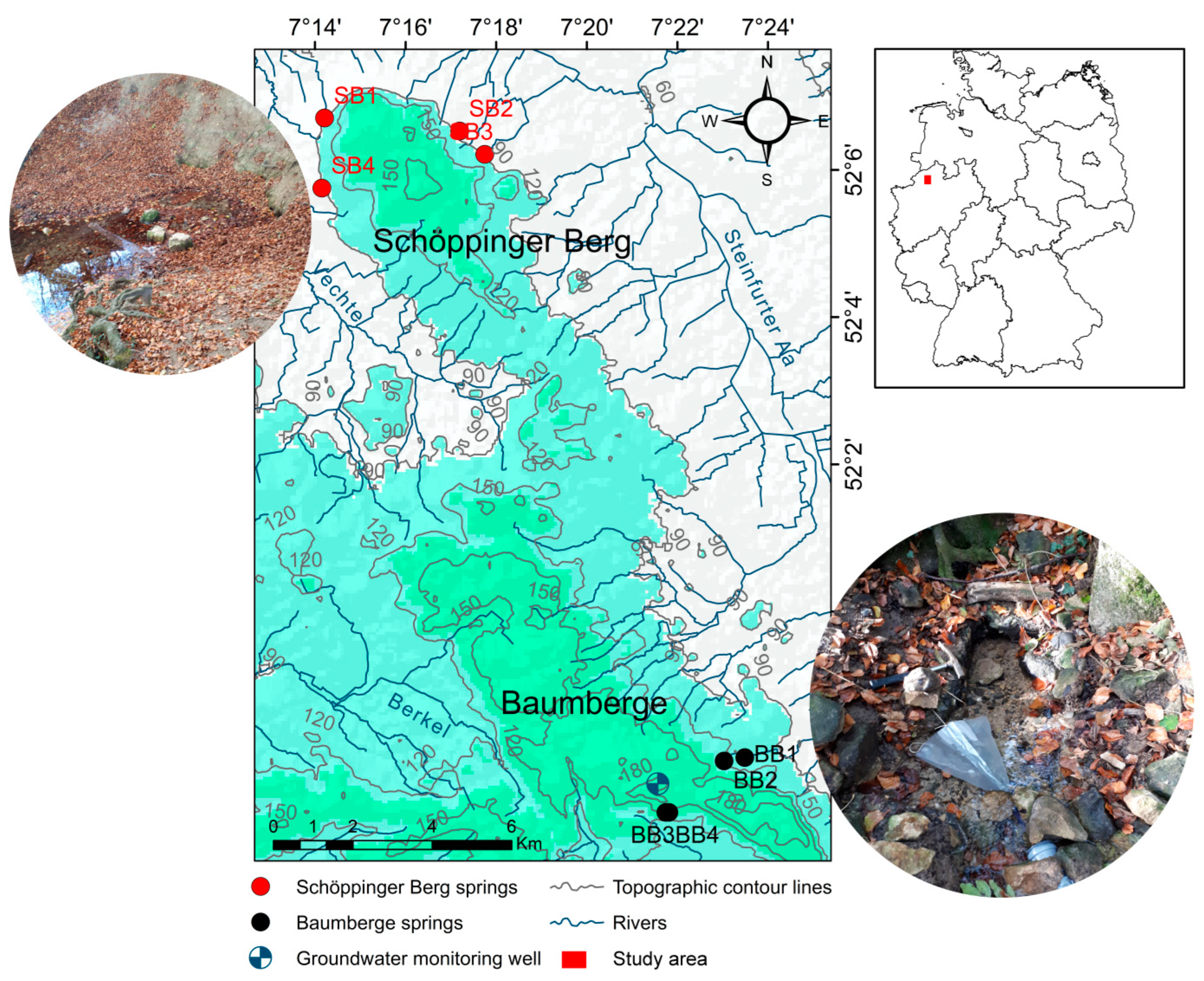
2.1. Study Area

Eight springs were investigated in two regions, Baumberge (BB) and Schöppinger Berg (SB), in North Rhine Westphalia western Germany, in central Münsterland (Figure 1). Baumberge and Schöppinger Berg are flat hilly areas with a maximum height of 186 and 157.6 m above mean sea level (m a.s.l), respectively. The areas consist of bowl-shaped curved porous and calcareous marlstone layers, which are fractured and slightly karstified. The two areas each form isolated groundwater ecosystems. Surface water features, with the exception of infiltrating rainwater, are almost absent except some intermittent rivers/creeks. Both areas are characterized by agricultural activities and have forested mountain slopes. For more geological and hydrogeological information about the two areas, readers are referred to [37] and references therein.

2.2. Methodology

Water was sampled from eight perennial natural springs distributed at the edge of the BB and SB regions, with four springs each (Figure 1). Fieldwork encompassing the measurement of physicochemical parameters, spring discharge, water sampling for aquatic invertebrates and detritus, and monitoring of the groundwater level took place in November 2018 (Nov.), April 2019 (Apr.), and October 2019 (Oct.); sampling lasted to 2–5 days in each sampling time campaign. For chemical, isotope, and biological analyses, spring water samples were collected in Nov., Apr., and Oct. This sampling time was conducted first to avoid short-term fluctuations and second because of technical and logistic issues. In total, there were 78 sampling events for physicochemical parameters and aquatic invertebrates and 24 sampling events for hydro(geo)chemical and microbiological analyses. Observation data of the groundwater table were taken from the observation well “Longinusturm” [latitude (lat.): 51°57′36″ N, longitude (lon.): 7°21′56″ E], which is considered a representative monitoring point in the area.

2.2.1. Field Work

Groundwater samples were collected during a one-year sampling period for different purposes from the spring discharges, and they were transported to the laboratory for biological and hydro(geo)chemical analyses.

Field Parameters and Aquatic Invertebrates Sampling

The field parameter and aquatic invertebrate sampling were conducted once daily every 2–5 days in each sampling campaign in each spring. Physicochemical parameters of sampled water pH value (pH; -), temperature (Temp.; °C), electrical conductivity (EC; µS/cm), and dissolved oxygen concentration (DO; mg/L)] were measured in situ using a multi-parameter field sensor (WTW 340i). The discharge of each sampled spring ( V ˙ ; L/s) and the fraction of spring discharge that flowed through the planktonic net were estimated on site. The groundwater table (hGW; m a.s.l.) was monitored once per sampling campaign with a water level meter of the type 100 LTC (HT Hydrotechnik GmbH, Obergünzburg, Germany).
Spring water with aquatic invertebrates, sediments, and detritus was captured with a planktonic net, with a mesh size of 74 µm. Plankton nets were installed against the selected outlet at a representative discharging point of each spring. After 24 h, the samples were washed and filtered with a mesh size of 74 µm. This mesh size is suitable for collecting invertebrates of a wide range of body sizes, including meiofauna. After filtration, the samples were stored in 100–1000 mL flasks in a cool box and transported under dark and cold conditions within half a day to the laboratory for additional analyses. These samples were stored live at 10 °C in a dark refrigerator and processed in the laboratory within one week of sampling. Then, the Groundwater-Fauna-Index (GFI) after Hahn [38] was calculated per sampling event.

Hydro(geo)chemical and Microbiological Sampling

Hydro(geo)chemistry and microbiology sampling was conducted once per sampling campaign each spring. The samples of groundwater to be evaluated for major cations (calcium: Ca2+, magnesium: Mg2+, sodium: Na+, potassium: K+, strontium: Sr2+, aluminum: Al3+, and iron: Fe2+) were collected in 100 mL vials and acidified with 3 drops of nitric acid (HNO3). Samples of groundwater for major anions (sulfate: SO42−, chloride: Cl, nitrate: NO3, phosphate: PO43−) were also collected in 100 mL vials. Samples of 500 mL were collected for bicarbonate (HCO3) analysis.
Samples for stable isotope analysis were collected in 100–1000 ml flasks and stored in cool and dark conditions. Water samples for nitrate isotopes were shock-frozen with liquid nitrogen immediately after sampling and stored until isotope measurements were carried out.
The microbiological analysis consisted of total counts of prokaryotic cells/biomass (TCC; cells/L) and quantification of intracellular adenosine triphosphate called activity (ATP; pM). For analysis of cell numbers, 50 ml of spring water was collected using latex gloves and fixed with glutaraldehyde (1) ml 25% GDA solution in 50 mL samples (=0.5% final concentration). For analysis of intracellular ATP, 50 ml samples were collected and processed as described by [39]. Samples were transported in a cool box and stored in the dark (refrigerator).

2.2.2. Laboratory Work

Further processing of the aquatic invertebrates and detritus is described in [37]. In the following, all aquatic invertebrate individuals (hereafter abbreviated as sf) were sorted into stygobites (sb) (smaller transparent individuals without eyes) and non-stygobites (non-sb) (stygoxenes and stygophiles).
The concentrations of major ions were determined by means of optical emission spectroscopy with inductively coupled plasma (ICP-OES with SPECTROBLUE TI, SPECTRO Analytical Instruments) and ion chromatography (IC with 761 Compact IC, Metrohm, Fielderstadt, Germany). Bicarbonate was determined by titration with 0.1 mL HCl to a pH of 4.3 (methyl orange as an indicator). Stable isotopes of water (δ2HH2O and δ18OH2O) were measured using the Triple Isotope Water Analyzer (TIWA-45-EP, Los Gatos Research). The stable isotope of dissolved inorganic carbon (δ13CDIC) was measured using an isotope ratio mass spectrometer (IRMS with MAT DeltaPlusXL) coupled with Gasbench II (Thermo Scientific). Nitrate isotopes (δ15NNO3 and δ18ONO3) were determined using the Gas Bench II coupled with mass spectrometer, after preserving the samples by shock freezing with liquid nitrogen. Sulfate isotopes (δ34SSO4 and δ18OSO4) were measured using high-temperature pyrolysis coupled with a mass spectrometer. The biomass (TCC) was determined by flow cytometry (FC500 CYTOMICS; Beckman Coulter, Brea, CA, USA), and activity (ATP) was measured using the BacTiter-Glo Microbial Cell Viability Assay kit (Promega, Madison, WI, USA) [39,40,41].

2.2.3. Data Processing

The groundwater table was considered constant during each sampling campaign. Physicochemical parameters were averaged over 2–5 days for each sampling campaign. In the case of aquatic invertebrates, the number of stygofauna per cubic meter of spring discharge was calculated as an average value related to the sampling period [37]. The measurement of δ15NNO3 and δ18ONO3 was carried out only in Nov. 2018 and April 2019. Missing data were handled appropriately at the beginning of the statistical analysis. Then, the Mann–Whitney U test was conducted between both springs, i.e., BB and SB.
The hydro(geo)chemical situation of the study areas was assumed according to the available measured data. The influence of environmental factors on the aquatic invertebrates and microbial parameters was tested using a Spearman correlation and principal component analysis (PCA). These statistical analyses were performed using the Statistical Package for Social Sciences Software SPSS.26 (IBM Corp. Released 2019. IBM SPSS Statistics for Windows, Version 26.0. IBM Corp.: Armonk, NY, USA). The analytical precision for cation and anion analyses was assessed by checking ion balance errors using Phreeqc, and it was generally within the range of ±5%. Saturation indices were calculated in Phreeqc interactive 3.7.3–15968 [42] and the wateq4f database. Maps were prepared in ArcMap (ArcGIS Desktop 10.8.1, Environmental Systems Research Institute (ESRI), Redlands, CA, USA) and the charts were prepared in Microsoft Excel 2016 (Microsoft Corporation 2016).

3. Results and Discussion

According to the Mann–Whitney U test, most of the biotic and abiotic parameters between the two groups of springs differ significantly (p ≤ 0.01). Therefore, the two groups of springs will be handled separately and compared with each other.

3.1. Physicochemical Parameters, Spring Discharge and Groundwater Table

Descriptive statistics of physicochemical parameters, Spring discharge and groundwater table in BB and SB are presented in Tables S1 and S2. The hGW fluctuated between the highest value of 122.82 m a.s.l. in Apr. and the lowest value of 114.30 m a.s.l. in Nov. 2018 and 114.24 m a.s.l. in Oct. 2019. The average daily V ˙ values were 21.71 and 15.90 m3/d in Apr. and 17.39 and 14.84 m3/d in Oct. 2019 in BB and SB, respectively. The fluctuation of V ˙ follows that of the hGW.
The average Temp. was in the range of 9.70–10.50 °C and 9.80–12.00 °C in BB and SB, respectively. The average pH was circumneutral (7.2), and it ranged from 7.0 to 8.0 and from 7.0 to 7.4 in BB and SB, respectively. The average EC was higher in SB than in BB, with values in the range of 700–757 µS/cm in BB and the range of 749–828 µS/cm in SB. The concentration of DO ranged between 4.65 and 7.50 mg/L in BB and between 4.77 and 8.60 mg/L in SB. The results of the descriptive statistics showed that Apr. was marked by higher values of EC and DO. This high value of EC in Apr. could be the result of higher Temp. Moreover, higher EC values were measured in SB compared to BB, which might be related to the elevated concentration of NO3 due to intensive agricultural activities [6].

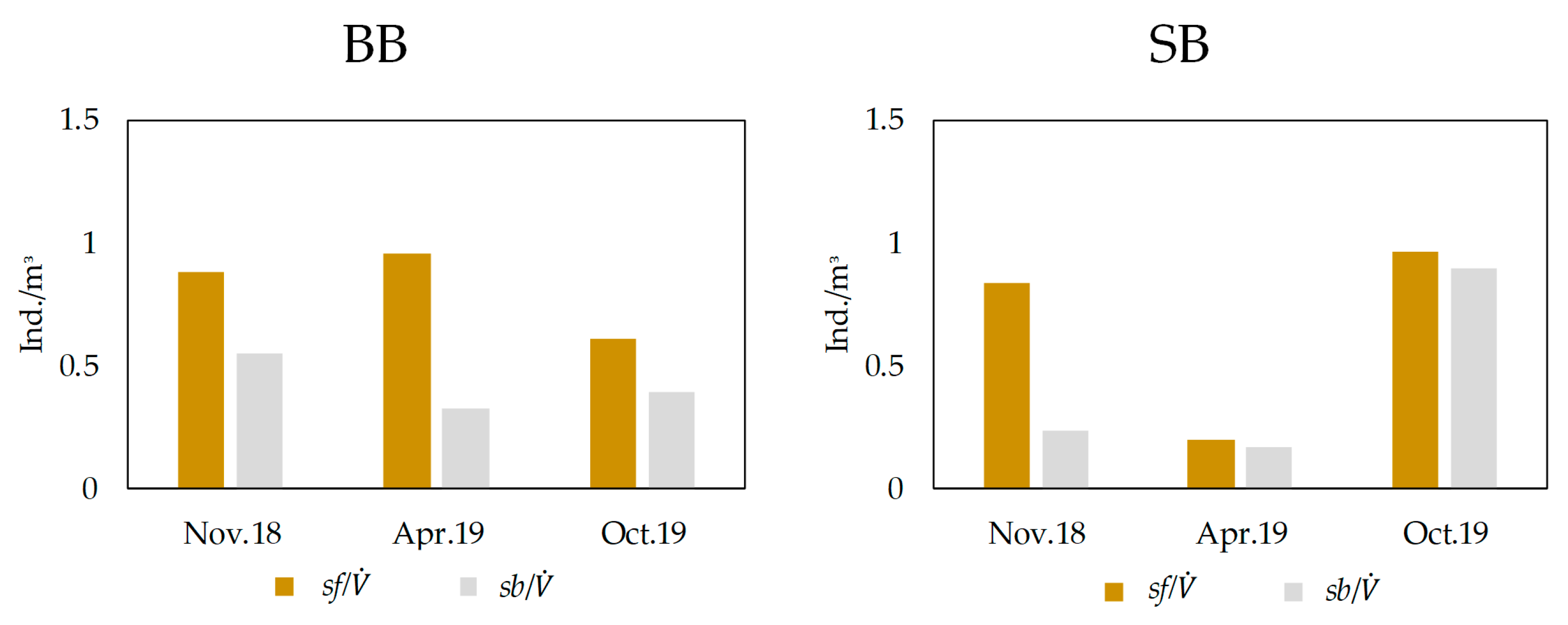
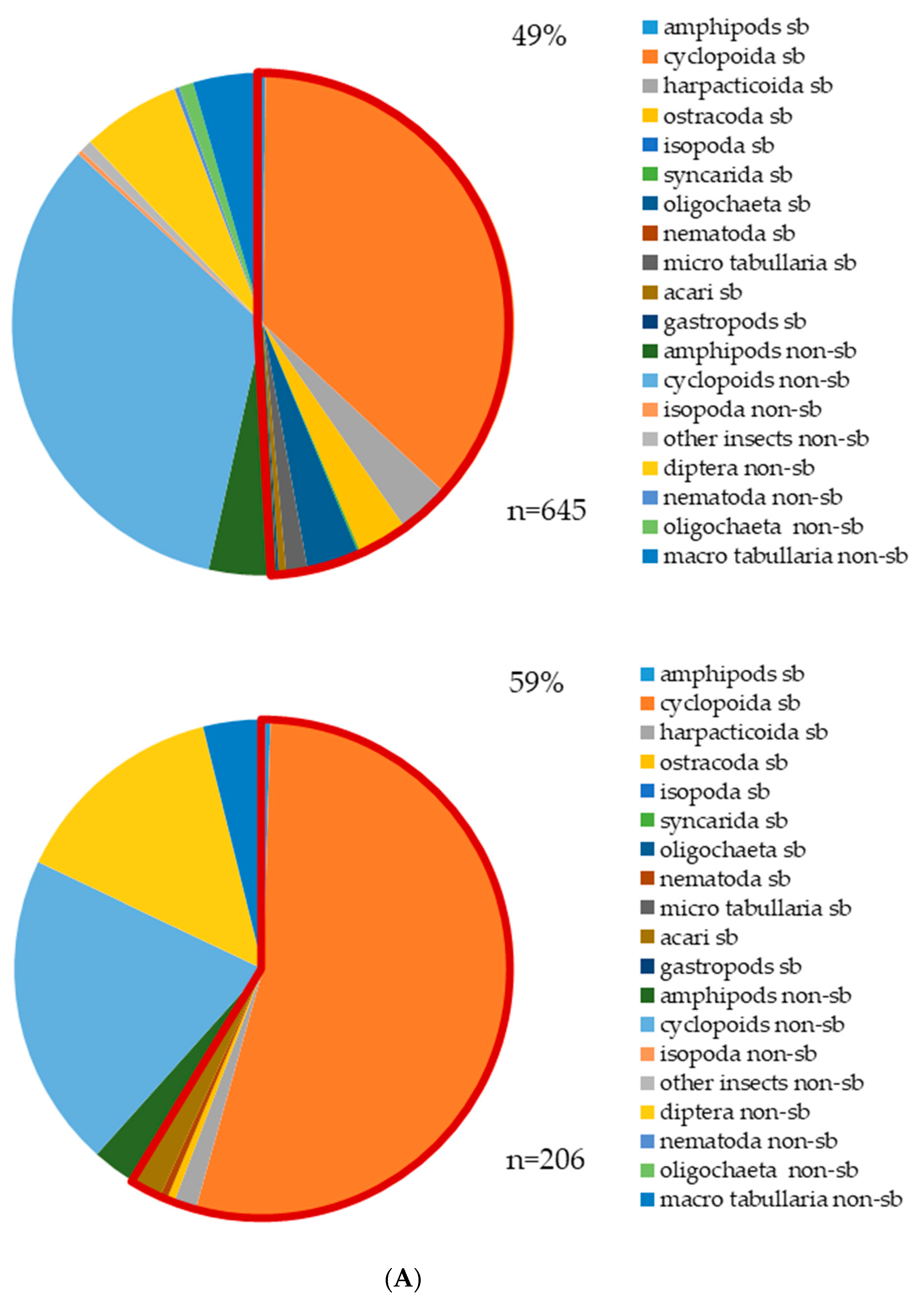
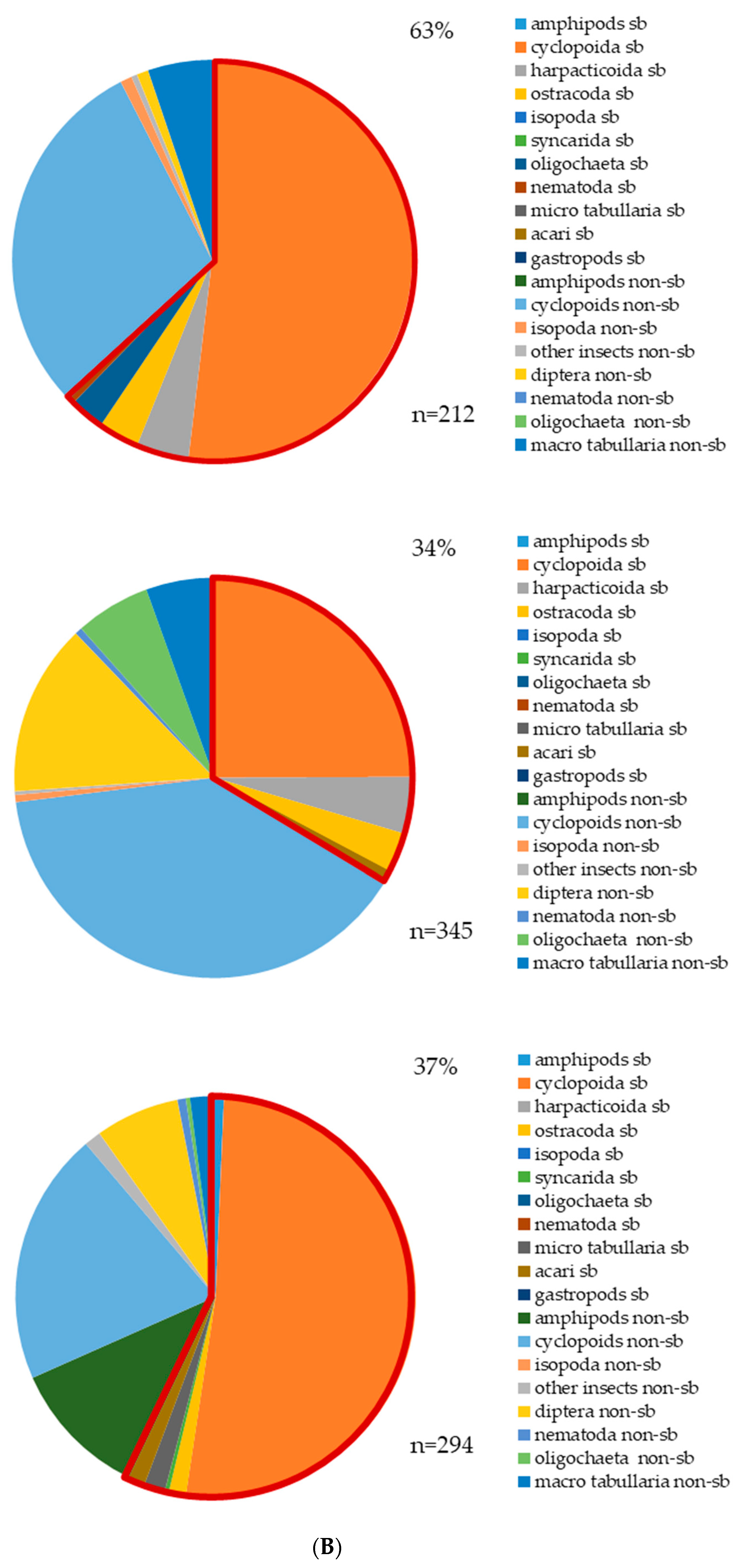
3.2. Aquatic Invertebrates (Stygofauna) and Stygobites

The total number of aquatic invertebrates measured in water samples of the eight springs in BB and SB from three sampling campaigns was 851 individuals (Ind.). The results showed that the average number of aquatic invertebrates (sf/ V ˙ ) and stygobites (sb/ V ˙ ) individuals per cubic meter (Ind./m3) varied over time and between the two study areas (Figure 2). In Apr., sf/ V ˙ in BB was nearly 1.0 Ind./m3, much higher than that in SB with 0.2 Ind./m3. In contrast, sb/ V ˙ in both BB and SB was the lowest in April 2019 at higher hGW and higher discharge, with nearly the same value of 0.3 Ind./m3 in BB and SB. In times of lower hGW in November 2018 and October 2019, the number of sb increased. In SB, the reproduction of the aquatic invertebrates in groundwater space seemed to increase at lower hGW, while in BB it increased at higher hGW [37].
The variability of aquatic invertebrates, which consist of sb and non-sb individuals, is an indicator of the diversity of aquatic invertebrates. Comparing the two study areas, the 645 individuals of BB in total could be assigned to 17 types or species. The group of sb individuals showed nine taxa, with 49% of all aquatic invertebrates. Among the sb individuals, sb cyclopoids were the dominant group (with 237 individuals) followed by harpacticoids and ostracods, while non-sb individuals showed only eight taxa. In contrast, only 206 individuals of SB in total could be assigned to 10 species. The group of sb individuals showed six taxa with 59% of all aquatic invertebrates. The dominant sb invertebrates were cyclopoids with 111 individuals. This means that the diversity of aquatic invertebrates and sb individuals during the sampling campaigns was higher in BB than in SB, but the percentage of sb individuals was higher in SB than in BB (Figure 3A).
Comparing the three sampling campaigns, the aquatic invertebrates sampled per campaign numbered 212 in November 2018, 345 in April 2019, and 294 in October 2019, with 8, 12, and 13 species, respectively. The sb individuals were in five taxa in November 2018, four taxa in April 2019, and six taxa in October 2019. The results showed that October 2019 was marked with the highest diversity and non-sb of three, eight, and seven taxa in Nov., Apr., and Oct., respectively. The percentage of sb individuals was the highest in November 2018 at 63% and the lowest in October 2019 and April 2019 at 37% and 34%, respectively (Figure 3B).

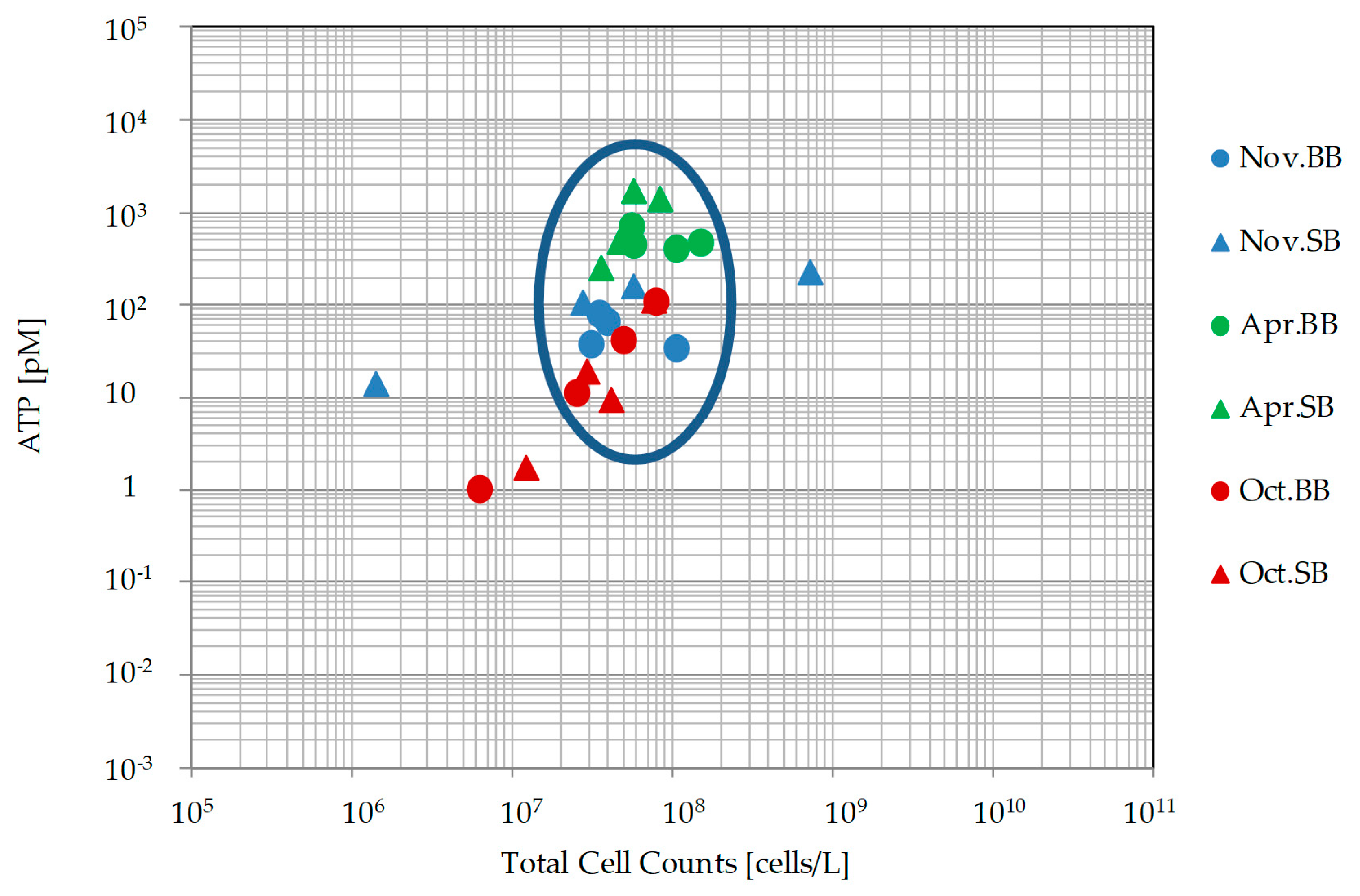
3.3. Microbiological Analyses (Biomass and Activity)

Water samples in BB showed that the biomass (total counts of prokaryotic cells; TCC) ranged from 6.23 × 10⁶ to 1.53 × 10⁸ cells/L, with an average of 6.21 × 10⁷ cells/L. In SB, TCC ranged from 1.41 × 10⁶ to 7.38 × 10⁸ cells/L, with an average of 1.01 × 10⁸ cells/L. The activity (the concentration of intracellular ATP) ranged from 9.70 × 10⁻¹ to 6.79 × 10² pM with an average of 1.96 × 10² pM in BB, and from 1.74 to 1.74 × 10³ pM with an average of 3.76 × 10² pM in SB (Tables S1 and S2). In the temporal view, TCC and ATP in Nov. 2018 ranged from 1.41 × 10⁶ to 7.38 × 10⁸ cells/L and from 1.42 to 2.25 × 10² pM, with an average of 1.30 × 10⁸ cells/L and 8.95 × 10 pM, respectively. In April 2019 they ranged from 3.58 × 10⁷ to 1.53 × 10⁸ cells/L and from 2.54 × 10² to 1.74 × 10³ pM with an average of 7.46 × 10⁷ cells/L and 7.30 × 10² pM, respectively. The values in October 2019 ranged from 6.23 × 10⁶ to 7.87 × 10⁷ cells/L and from 9.70 × 10⁻¹ to 1.13 × 10² pM, with averages of 4.03 × 10⁷ cells/L and 3.80 × 101 pM, respectively.
In April 2019, when the groundwater level was high at the end of the groundwater recharge phase, water samples had the highest and most uniform cell activity, ranging from 2.54 × 10² to 1.74 × 10³ pM, with high cell counts of 3.58 × 10⁷ to 1.53 × 10⁸ cells/L across all springs. This points to the fact that groundwater at this time shows very uniform ecological conditions, i.e., little spatial variation. The high cell count indicates fast recharge is taking place, which drives cells from the surface to the groundwater ecosystem. There were also probably sufficient nutrients present. The ATP at the end of the groundwater depletion phase in November 2018/October 2019 was low everywhere with more or less comparable numbers of cells (not taking into account the four outliers: November 2018, SB1, SB4, and October 2019, SB3, BB4). However, the number of cells varied considerably, and, thus, there are stronger spatial variations with more heterogeneous ecological conditions in a phase with reduced groundwater volume.
The overall TCC and ATP data were significantly positively correlated in November 2018 and October 2019 with correlation coefficients of r = 0.9 and 0.58 (p ≤ 0.05), respectively. These were, however, not correlated in April 2019 (r = 0.008; p ≤ 0.05). This might indicate that most cells in November 2018 were active and contained similar amounts of ATP. In other words, a good correlation between TCC and ATP indicates growth in the system, while a lack of correlation indicates starvation or the introduction of cells from outside. As mentioned before, the case in April 2019 was related to rising hGW. Figure 4 shows that, with some exceptions (samples outside the blue oval), there was a shift in ATP rather than a shift in TCC. The activity was lower in November 2018 (autumn), while it increased in April 2019 (spring) when recharge takes place and nutrients (DOC) are washed into the groundwater ecosystem, which stimulates cell activity (high ATP content). At the same time, not much growth was taking place (cell counts did not change much), and there is no indicator that cells were washed in. The ATP dropped again until October 2019 (autumn). With one exception, the same applies to TCC, which tended to be lower in November 2018 and October 2019 than in April 2019. This could be explained by the fact that during the recharge time, nutrients transported into the system allow cells to become more active, and/or some cells are transported from the surface into the groundwater system. Analyzing data on the main threats to groundwater ecosystems, i.e., agricultural activities, shows that microbial cell density can exhibit a delayed response to nutrient inputs [43], which causes an increase in TCC without changes in ATP. This would be the case if cells from the infiltration rainwater were transported into the groundwater but were inactivated by the characteristically lower nutrient levels in the groundwater compared to flow water [39].

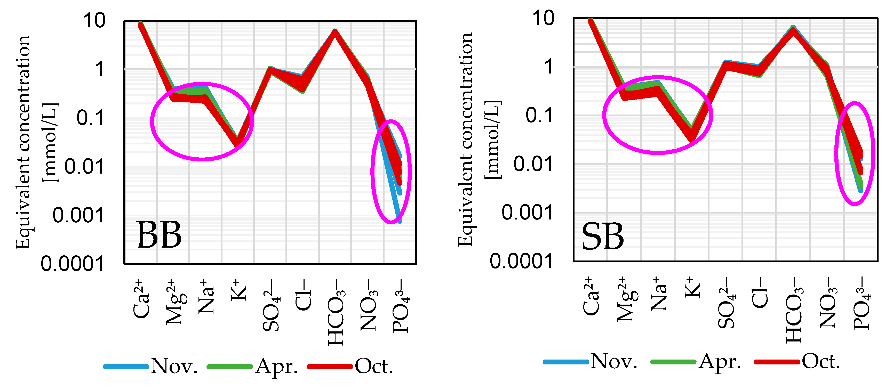
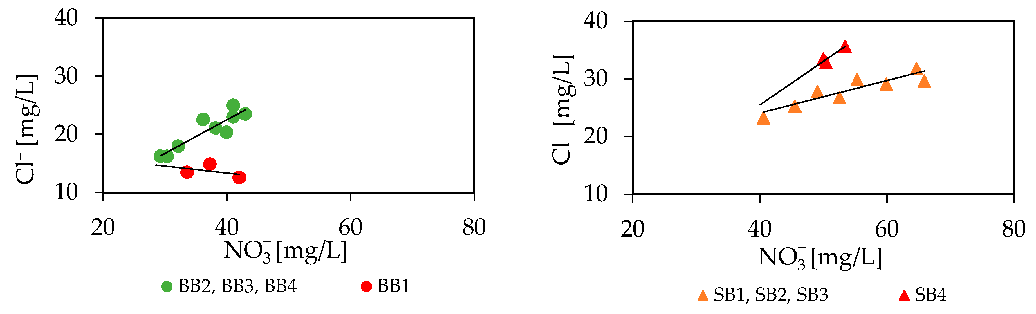
3.4. Groundwater Hydro(geo)chemistry

The relative abundances of major cations in groundwater within the study areas were in the order Ca2+ > Mg2+ > Na+ > K+, while the major anions were in the order HCO3 > SO42− > Cl. Concentrations of Ca2+, Mg2+, Na+, and K+ in BB springs were in the range of 154.6–172.2 mg/L, 2.91–4.76 mg/L, 5.05–9.89 mg/L and 1.00–1.28 mg/L, respectively. In SB, the concentrations of these cations were in the range of 168.5–187.0 mg/L, 2.7–4.68 mg/L, 6.27–10.91 mg/L, and 1.16–1.98 mg/L, respectively. Nitrate, SO42− and Cl were in the range of 342.21–373.48 mg/L, 41.70–50.5 mg/L, and 12.59–25 mg/L in BB and in the range of 317.2–393.97 mg/L, 46.02–59.74 mg/L and 23.19–35.64 mg/L in SB, respectively (Tables S1 and S2). The average concentrations of major cations and anions in groundwater during the three sampling months were almost constant. The dominant cation and anion were Ca2+ and HCO3 (Figure 5), in agreement with the carbonate lithology of the aquifer. Using Phreeqc [42] and applying the wateq4f database, all water samples had a saturation index of calcite (SIcalcite) in the range of 0.03–1.00. This means that groundwater in both areas was oversaturated with CO2, resulting in CaCO3 dissolution. In Figure 5, Mg2+, Na+, K+, NO3, and PO43− show temporal variations (pink oval). The average concentration of nitrate (NO3) and phosphate (PO43−) was higher in SB (NO3 = 53.5, PO43− = 0.21 mg/L) compared to BB (NO3 = 37 mg/L, PO43− = 0.19 mg/L). The high concentrations of NO3 in both regions are most likely related to land use and agricultural activities [26]. The average concentration of PO43− increased with time in SB and BB (Figure 5) but was, in general, low.
Apart from denitrification, NO3 is thought to be conservative in groundwater, the same as Cl and bromide (Br) [44]. Thus, the correlation between NO3 and Cl can be informative regarding possible sources of NO3 in groundwater for BB and SB (Figure 6). In general, a positive correlation between NO3 and Cl is significant in both areas but at different levels. In BB, the concentrations of NO3 and Cl were lower than in SB. The variation range of Cl was the same with 12 mg/L in both areas. In BB, one spring (BB1) showed nearly constant Cl level with increasing NO3 concentration. This line parallel to the X-axis might be affected by denitrification [43]. In SB, one spring, SB4, showed a higher Cl level at a similar NO3 concentration. Compared to the other springs in SB, SB4 is located in a more urban area.

3.5. Stable Isotope Signatures in Spring Water

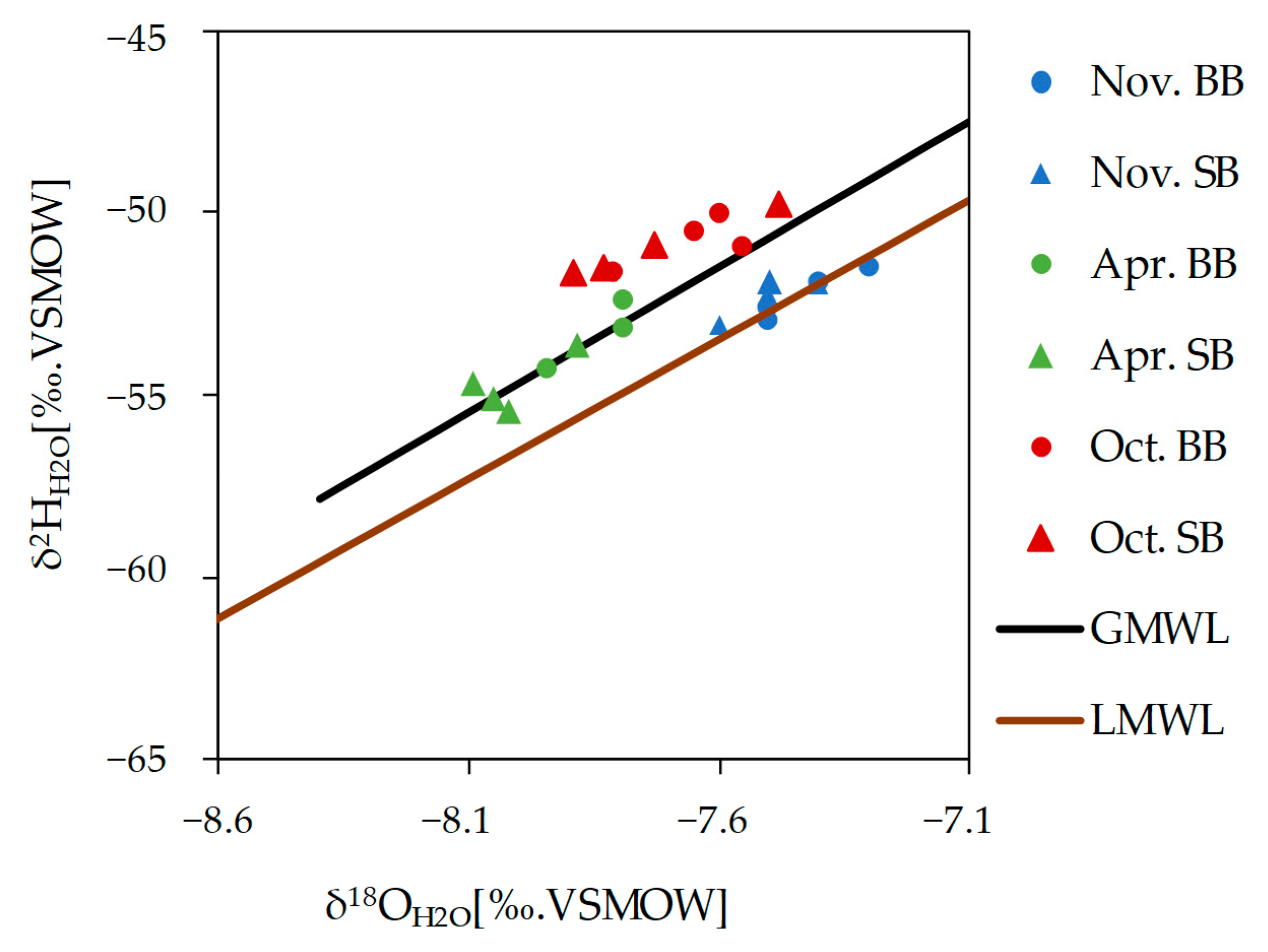
3.5.1. Stable Isotopes of Water (δ2H and δ18O)

The spring water samples display variations between −55.49‰ and −49.8‰ for δ2H and from −8.1‰ to −7.3‰ for δ18O (Tables S1 and S2). The stable isotopic signatures of spring water show a significant temporal variation and can be separated into three groups. The first group (October 2019) consists of less depleted samples, and these are located above the GMWL for both areas. The second group (November 2018) is positioned almost on the LMWL. The trend of the samples of these two groups shows an inclination to the right of the LMWL. The third group (April 2019) exhibits more depleted values located on the GMWL, with a trend parallel to the GMWL (Figure 7).
The most depleted isotopic signatures of δ18O and δ2H were recorded in April 2019, at the end of the groundwater recharge period, at the highest hGW. These low isotope values reflect winter recharge (precipitation under cold conditions). The samples were enriched in Nov. 2018 at the lowest level of the groundwater table. Summer 2018 was one of the warmest and driest summers in North Rhine Westphalia [47], with a low groundwater table of 113.91 m a.s.l until December 2018 [48]. In Oct. 2019, at the end of the groundwater depletion phase at lower groundwater levels, the δ18O values showed medium values. Summer 2019 was also one of the hottest summers on record [47]. Over the last two months, this enrichment was the result of evaporation under non-equilibrium conditions at different temperatures and humidity, which is supported by the slope of the samples lower than that of the LMWL.

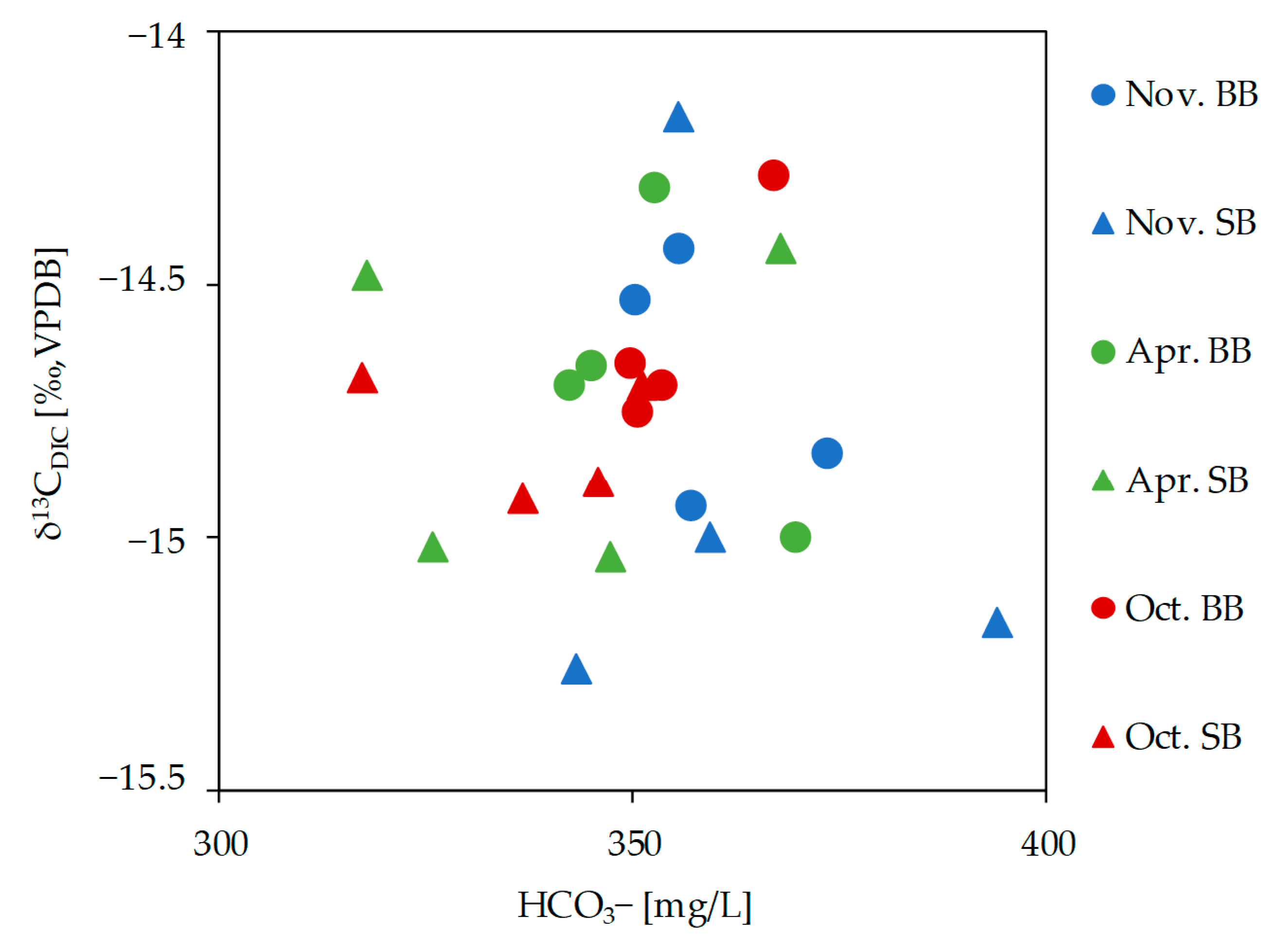
3.5.2. Stable Isotope of Dissolved Inorganic Carbon (δ13CDIC)

The values of δ13CDIC fluctuated within a narrow range from −15.26 to −14.17‰ with an average of −14.75 ‰ in BB, while in SB, they ranged from −15.04 to −14.43‰ with an average of −14.73‰ (Tables S1 and S2). Different sources of DIC exist in groundwater, such as atmospheric and soil CO2, oxidation of organic matter, and water–rock interactions [18]. The pH values were in the range of 7–8, which means that DIC is mainly composed of bicarbonate (HCO3) [49,50]. The oversaturation with CO2 results in the dissolution of carbonate rocks. Figure 8 shows the relationship between HCO3 and δ13CDIC in the water samples, with no significant correlation (p = 0.7). Values of δ13CDIC in groundwater reflect the dissolution of the carbonate aquifer rocks via carbonic acid resulting from the oxidation of organic matter in the overlying soil [5].

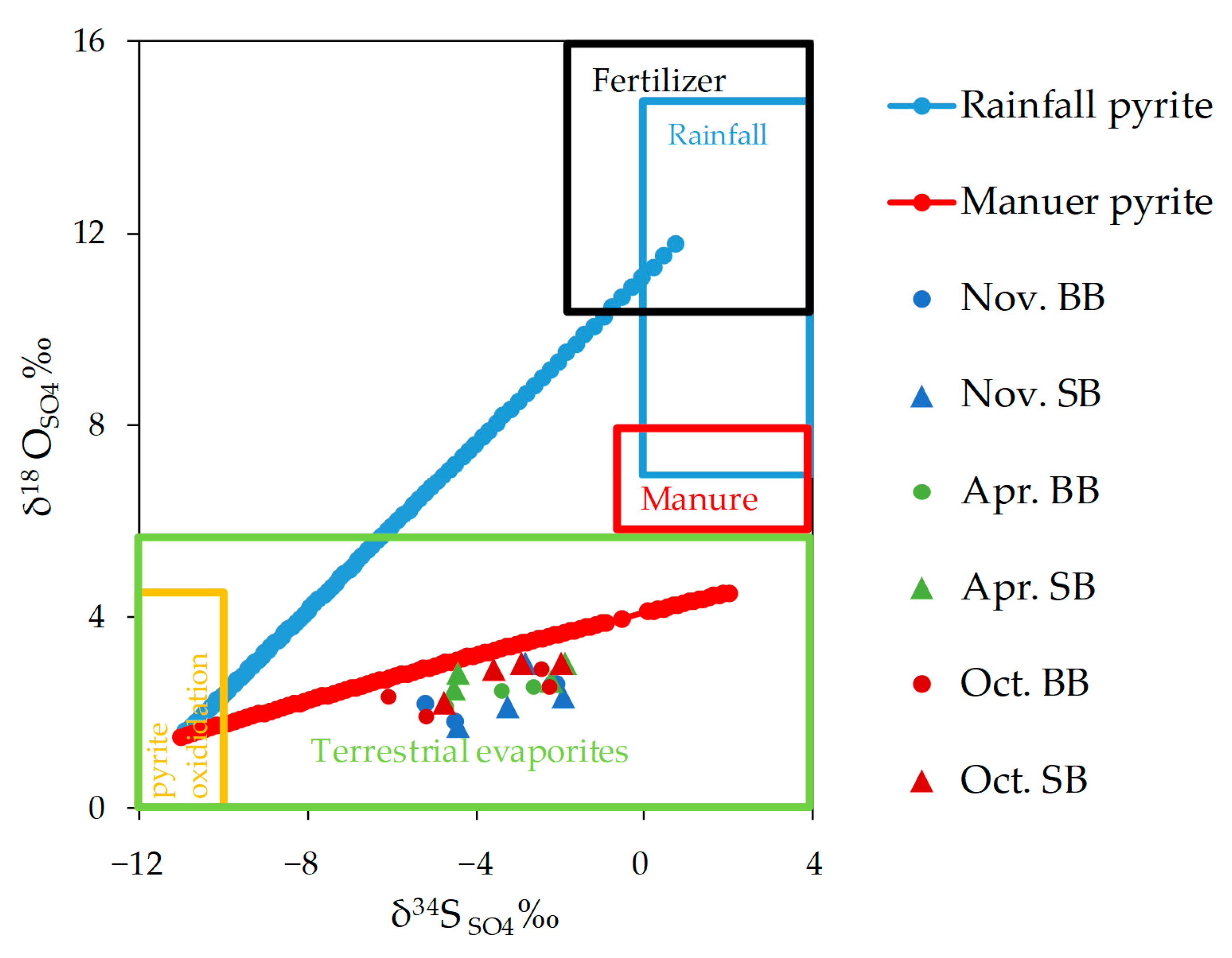
3.5.3. Stable Isotopes of Sulfate (δ34SSO4 and δ18OSO4)

The stable isotopes of sulfate range from −5.2‰ to −1.9‰ for δ34SSO4 and from 1.7‰ to 3‰ for δ18OSO4 in water samples from BB, and from −6.07‰ to −1.85‰ for δ34SSO4 and from 1.9‰ to 3.02‰ for δ18OSO4 in water samples from SB (Tables S1 and S2). There was no significant enrichment of both δ18OSO4 and δ34SSO4 in groundwater sulfate, which would be an indicator of microbial sulfate reduction [51]. This is also supported by the absence of a significant correlation (BB: r = 0.3; p = 0.4; SB: r = −0.3; p = 0.4) between SO42− and HCO3in the water samples.
The dual isotopes δ34SSO4 and δ18OSO4 in the spring water samples from BB and SB are plotted in Figure 9. The water samples are located between the two end members of pyrite oxidation and manure [52]. According to [53], the samples of BB and SB are located in the region of terrestrial evaporites, which covers a wide range of δ34SSO4 (−15‰–+10‰). This would support the aforementioned hypothesis (dissolution of secondary gypsum) for the observed correlation in water samples from SB. However, the question is still open for the spring water samples from BB and further research is needed in this regard. Particulate organic matter residing in the groundwater zone has been identified as a main electron donor, but additional contributions from the oxidation of reduced inorganic substrates such as pyrite cannot be excluded [52,54].
Surprisingly, there exists a significant positive correlation (r = 0.6, p = 0.07) between Ca2+ and SO42− in water samples in SB. This significant correlation could point to gypsum dissolution. However, gypsum has not been documented in the regional stratigraphy of the BB/SB areas. Using Phreeqc calculation, SIgypsum of the collected water samples was in the range (−0.3)–(−1), which is close to equilibrium. This raises the question of whether precipitation/dissolution of secondary gypsum might control the SO4−2 concentration in SB. Secondary gypsum is well-known in soils of arid and semi-arid areas [57]. Precipitation of secondary gypsum could take place in the unsaturated zone due to evapoconcentration. This hypothesis considers a source of SO42− from the surface. This surficial source of SO42− is supported by the positive significant correlation (r = 0.9; p < 0.01) between SO42− and Cl. With time, SO42− percolates downward and cycles of precipitation/dissolution of secondary gypsum increase SO42− in groundwater. The same, however, does not apply to BB, and this reflects an overlap of different processes which affect the hydro(geo)chemical situation.

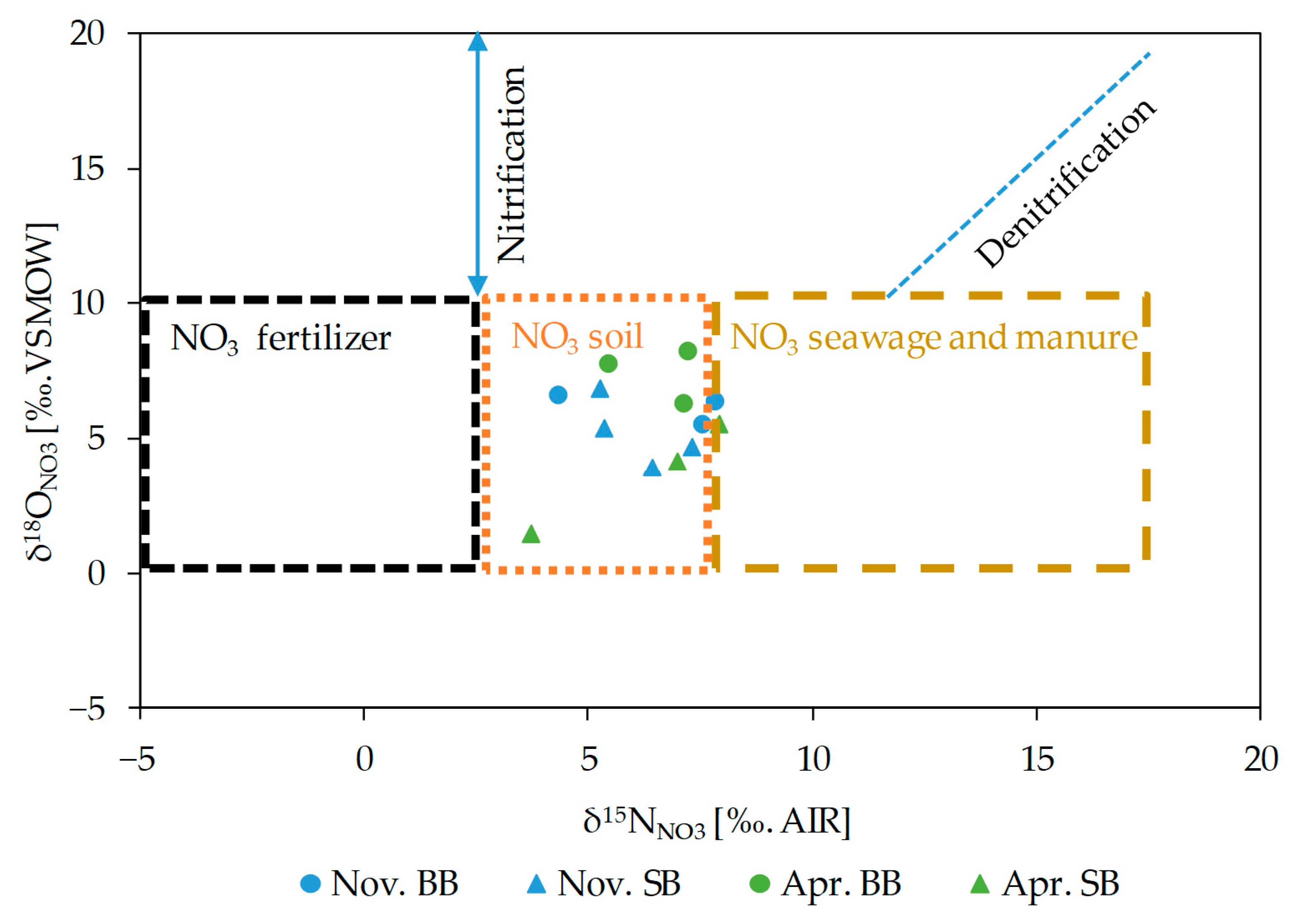
3.5.4. Stable Isotope of Nitrate (δ15NNO3 and δ18ONO3)

The average nitrate concentration in spring water samples of BB (37 mg/L) was less than that of SB (54 mg/L) (Tables S1 and S2). The isotopes of nitrate had an average value of 5.8‰ δ15NNO3 and 6.1‰ δ18ONO3 in BB, and 6.1‰ δ15NNO3 and 4.6‰ δ18ONO3 in SB. The values of δ18ONO3 in BB and SB ranged from +1.5 to +8.3‰, indicating that atmospheric NO3 deposition (+55 to +75‰) was not a dominant source of NO3 to groundwater in BB and SB. Values of δ15NNO3 (+2.8 to +7.9‰) and δ18ONO3 (+1.5 to +8.3‰) reflect soil nitrate and a possible contribution from sewage and manure, but no contribution through NO3 fertilizer (Figure 10).

3.6. Statistical Analyses

For a better understanding of the quality of the data and the reliability relationship between parameters, a Spearman correlation matrix and principal component analysis were applied to the data to summarize the patterns in environmental variables. The diversity of aquatic invertebrates, pH value, and stable isotopes of nitrate (δ15NNO3 and δ18ONO3) were not considered in the statistical analyses.

3.6.1. Spearman Correlation

Spearman correlation assesses monotonic relationships. The correlation was conducted for BB and SB between 12 samples of 30 variables, considering a significance level of p ≤ 0.01. The correlation results (Tables S3 and S4) showed that ATP in BB and SB was significantly positively correlated with hGW, which is explained by the fast groundwater recharge and simultaneous nutrient input. In SB, this ATP was significantly positively correlated with Al3+, and significantly negatively correlated with δ2HH2O and PO43−. This negative correlation with PO43− is not easy to justify in light of the available data, because many factors affect PO43− release into/availability in groundwater. It is worth mentioning that phosphate tends to be absorbed into the soil and is not readily transported into groundwater [60], and its release is enhanced under anoxic conditions [61]. The inverse correlation of ATP with δ2HH2O is likely due to the enrichment of water isotopes under the influence of evapotranspiration on the surface/in the unsaturated zone; however, this signature is not reflected in the relationship between ATP and δ18OH2O. In BB and SB, the aquatic invertebrates (sf/ V ˙ ) were significantly positively correlated with stygobites (sb/ V ˙ ). As was stated in previous studies [43], aquatic invertebrates, TCC, and ATP were not correlated at the significance level of p ≤ 0.01. A significant negative correlation existed between stygobites (sb/ V ˙ ) and SO42− and Cl in SB. Fluctuation of the groundwater table was significantly positively correlated with Sr2+ and Fe2+, and significantly negatively correlated with PO43− only in SB. Aquatic invertebrates, TCC and ATP showed rare and inconsistent relationships with individual physicochemical and hydro(geo)chemical parameters of water samples in BB and SB, as was stated in previous studies [38,62].

3.6.2. Principal Component Analysis

Principal component analysis was applied to reduce the number of variables. The significance of the loadings was obtained at p ≤ 0.01. Before processing, data vectors were normalized to a mean value of zero and a standard deviation of one. The presence or absence of any influence of a specific parameter on the investigated variables could be inferred from similarities and variations in the studied variables. From the abiotic and biotic parameters (30 variables) of 12 spring samples, five principal components (PCs) were extracted, explaining 82.2% and 84.2% of the total variance for BB and SB, respectively. High positive loadings (Pearson correlation coefficient) of different variables on the same principal components may indicate a close relationship among the respective variables, whereas negative loadings between variables indicate an inverse relationship.
For BB, the percentages of variance explained by the five principal components were 25.42% for PC1, 22.23% for PC2, 14.68% for PC3, 11.71% for PC4, and 8.14% for PC5 (Table 1). The positive loading of Na+, Mg2+, and Sr2+, and the negative loading of SiO32− on the first principal component (PC1) show (hydro)geogenic influences from the easier incongruent dissolution of carbonates in the BB groundwater ecosystem, which increases when recharge decreases due to the increase in residence time. The negative loading of SiO32− on PC1 indicates the slower dissolution of SiO32− from kaolinite (average SIKaolinite = 2) in the unsaturated zone through recharge moving downward. The positive loading of NO3, Ca2+, and negative loading of SO42− with detritus in PC2 shows the anthropogenic influences (application of fertilizers and sewage/manure) on the groundwater ecosystem, and this component could indicate the different origins of NO3 and SO42−, providing distinct signatures. The third component (PC3) shows significant positive loadings of hGW and ATP and a negative loading of δ18OH2O. The positive loading of hGW and ATP is explained by input of nutrients together with fast groundwater recharge and the decrease in the vadose zone thickness, which induces more microbial ingress from the surface. The negative loading of δ18OH2O is most likely due to recharge either from snow melting or precipitation or recharge with no effect of evaporation from raindrops, which in turn induces higher hGW. The fourth component (PC4) shows significant negative loadings of Cl, V ˙ and positive loading of HCO3, which is indicative of the dissolution of the aquifer matrix during slow groundwater flow with minimal exchange with the ground surface. Phosphate, GFI, sf/ V ˙ and sb/ V ˙ load positively on PC5, indicating an increase in the abundance of aquatic invertebrates and stygobite individuals with an enhanced influence from the surface, reflecting an intensive interaction with the surface at high groundwater level [38,62], which provides PO43− as a nutrient for aquatic fauna, especially when the content does not exceed 1.0 mg/L [63].
In the case of SB, the percentages of variance explained by the principal components are 29.96% for PC1, 22.20% for PC2, 12.8% for PC3, 11.03% for PC4, and 8.11% for PC5 (Table 2). In SB, the first principal component (PC1) showed positive loadings of EC, K+, Ca2+, and Temp., and negative loadings of δ34SSO4, detritus, and δ18OSO4. These loadings mostly indicate the interaction between groundwater and minerals (carbonate, potassium-rich clays, terrestrial evaporites, and secondary gypsum) in the aquifer. The PC2 shows negative loadings from DO, hGW, and ATP, with positive loading of δ18OH2O and δ2HH2O. The lower groundwater table causes less interaction with the surface and thus less potential for higher ATP and DO, while stable isotopes of water tend to be enriched due to long infiltration distance and more evapoconcentration. The third principal component (PC3) shows significant positive loadings of Na+ and Mg2+, and negative loadings of SiO32−; which indicates the same geogenic influences as in BB. The stable isotope of dissolved inorganic carbon (δ13CDIC), Fe2+, and Al3+ load positively on PC4. This component is explained by the dissolution of clays under the influence of carbonic acid resulting from carbonate dissolution which causes enrichment in δ13CDIC [64]. Chloride loads positively and sb/ V ˙ loads negatively on PC5, which is an indicator of anthropogenic influence (sewage and manure) that increases Cl, which negatively affects the abundance of stygobite individuals.

4. Conclusions

This research study showed that the microbial and faunal patterns corresponded clearly to dynamics in hydrogeology and hydrochemistry, as the statistical evaluation showed. The relationships between the selected parameters are not clear-cut and vary somewhat across the areas. In a fractured and slightly karstified aquifer, a combined investigation of stygobites per cubic meter, microbial activity, groundwater table (or spring discharge), stable isotopes of water, dissolved oxygen, detritus, Groundwater-Fauna-Index, phosphate, and chloride as key parameters is recommended. Stable isotopes of inorganic carbon, sulfate, and nitrate as possible indicators of geochemical and microbial processes in the groundwater ecosystem were not shown to be key parameters for the ecological evaluation of the groundwater system in both areas.
The hydro(geo)chemical results showed no important spatial variation of the major ions of Baumberge and Schöppinger Berg. Only a few ions showed very low temporal fluctuations, such as sodium, magnesium, potassium, phosphate, and chloride. Hydrochemical parameters and stable isotopes revealed that the hydro(geo)chemical evolution of the groundwater is mainly affected by water–rock interactions. Precipitation contributes most of the recharge to the groundwater system, as supported by the stable isotopes of water. These also showed monthly fluctuations, with a clear effect of evaporation before infiltration, despite a high infiltration rate in the study area.
Nevertheless, stable isotopes of nitrate refer to the natural pollution by mineralization of soil organic nitrogen and, to a lesser extent, anthropogenic contamination from sewage water and manure. The previously proposed pyrite oxidation as a source of sulfate could not be confirmed on the basis of the selected sampling time. The results of stable isotopes confirm an agricultural influence on the groundwater ecosystem. Hydro(geo)chemical and isotopic analyses do not show that denitrification happens in the groundwater system in both areas.
To our knowledge, this is the first combined investigation of the spatial and temporal patterns of aquatic invertebrate and microbial parameters with physicochemical aspects and stable isotope investigation in the scientific community in this study area. The data presented reveal that the fluctuating hydrogeological conditions (readable from the groundwater level or spring discharge) exhibit pronounced temporal changes, especially in the stable isotopes of water, microbial information (activity), and stygobite individuals per volume. However, sampling adjusted to the groundwater level is highly recommended to cover the different hydrogeological conditions of the groundwater ecosystem in the area. Monitoring for successive years is also important to confirm the indicated temporal trends.

Supplementary Materials

The following supporting information can be downloaded at: https://www.mdpi.com/article/10.3390/geosciences13050140/s1, Table S1: Descriptive statistics of Baumberge on three sampling occasions; Table S2: Descriptive statistics of Schöppinger Berg on three sampling occasions; Table S3: Spearman correlation of BB, n = 12 samples of 30 variables, considering a significance level of p ≤ 0.01; Table S4: Spearman correlation of SB, n = 12 samples of 30 variables, considering a significance level of p ≤ 0.01.

Author Contributions

Conceptualization, S.A.A. and P.G.; fieldwork, S.A.A.; data curation, S.A.A. and P.G.; funding acquisition, S.A.A.; methodology, S.A.A., W.K., H.S. and P.G.; resources, S.A.A. and P.G.; supervision, P.G.; writing—original draft, S.A.A., W.K. and P.G.; writing—review and editing, S.A.A., W.K., H.S. and P.G. All authors have read and agreed to the published version of the manuscript.

Funding

This work was funded by the Hans Böckler Foundation.

Data Availability Statement

No data available.

Acknowledgments

I am grateful for financial support through individual doctoral funding from Hans Böckler Foundation. I am indebted to Christian Griebler for the inspiring, generous, and stimulating discussions, and his group in groundwater ecology in Munich and Vienna for microbial analysis. Our thanks go to the anonymous reviewers who helped to improve this article.

Conflicts of Interest

The authors declare no conflict of interest.

References

  1. Prasad, B.; Narayana, T. Subsurface Water Quality of Different Sampling Stations with Some Selected Parameters at Machilipatnam Town. Nat. Environ. Pollut. Technol. 2004, 3, 47–50. [Google Scholar]
  2. Gamar, A.; Zair, Z.; El Kabriti, M.; El Hilali, F. Study of the impact of the wild dump leachates of the region of El Hajeb (Morocco) on the physicochemical quality of the adjacent water table. Karbala Int. J. Mod. Sci. 2018, 4, 382–392. [Google Scholar] [CrossRef]
  3. Hose, G.C.; Symington, K.; Lategan, M.J.; Siegele, R. The Toxicity and Uptake of As, Cr and Zn in a Stygobitic Syncarid (Syncarida: Bathynellidae). Water 2019, 11, 2508. [Google Scholar] [CrossRef]
  4. Conrad, J.E.; Hirata, R.; Johansson, P.O.; Nonner, J.C.; Romijn, E.; Weaver, J.M.C. Groundwater Contamination Inventory: A Methodological Guide; Zaporozec, A., Ed.; UNESCO: Paris, France, 2002. [Google Scholar]
  5. Stein, H.; Kellermann, C.; Schmidt, S.I.; Brielmann, H.; Steube, C.; Berkhoff, S.E.; Fuchs, A.; Hahn, H.J.; Thulin, B.; Griebler, C. The potential use of fauna and bacteria as ecological indicators for the assessment of groundwater quality. J. Environ. Monit. 2010, 12, 242–254. [Google Scholar] [CrossRef]
  6. Aksever, F.; Davraz, A.; Karagüzel, R. Relations of hydrogeologic factors and temporal variations of nitrate contents in groundwater, Sandıklı basin, Turkey. Environ. Earth Sci. 2015, 73, 2179–2196. [Google Scholar] [CrossRef]
  7. Ma, F.; Chen, J.; Chen, J.; Wang, T.; Han, L.; Zhang, X.; Yan, J. Evolution of the hydro-ecological environment and its natural and anthropogenic causes during 1985–2019 in the Nenjiang River basin. Sci. Total Environ. 2021, 799, 149256. [Google Scholar] [CrossRef]
  8. Nisi, B.; Raco, B.; Dotsika, E. Groundwater Contamination Studies by Environmental Isotopes: A review. In Threats to the Quality of Groundwater Resources: Prevention and Control; Scozzari, A., Dotsika, E., Eds.; Springer: Berlin/Heidelberg, Germany, 2016; pp. 115–150. ISBN 978-3-662-48596-5. [Google Scholar]
  9. Sankoh, A.A.; Derkyi, N.; Frazer-williams, R.; Laar, C.; Kamara, I. A Review on the Application of Isotopic Techniques to Trace Groundwater Pollution Sources within Developing Countries. Water 2022, 14, 35. [Google Scholar] [CrossRef]
  10. Brunke, M.; Gonser, T.O.M. The ecological significance of exchange processes between rivers and groundwater. Freshw. Biol. 1997, 37, 1–33. [Google Scholar] [CrossRef]
  11. Soulsby, C.; Malcolm, R.; Gibbins, C.; Dilks, C. Seasonality, water quality trends and biological responses in four streams in the Cairngorm Mountains, Scotland. Hydrol. Earth Syst. Sci. 2001, 5, 433–450. [Google Scholar] [CrossRef]
  12. Ma, J.; Ibekwe, M.A.; Yang, C.H.; Crowley, D.E. Bacterial diversity and composition in major fresh produce growing soils affected by physiochemical properties and geographic locations. Sci. Total Environ. 2016, 563–564, 199–209. [Google Scholar] [CrossRef]
  13. Wright, J.; Kirchner, V.; Bernard, W.; Ulrich, N.; McLimans, C.; Campa, M.F.; Mackelprang, R. Bacterial community dynamics in dichloromethane-contaminated groundwater undergoing natural attenuation. Front. Microbiol. 2017, 8, 2300. [Google Scholar] [CrossRef] [PubMed]
  14. Kolar, B. The threshold concentration for nitrate in groundwater as a habitat of Proteus anguinus. Nat. Slov. 2018, 20, 39–42. [Google Scholar]
  15. Brkić, Ž.; Kuhta, M.; Larva, O.; Gottstein, S. Groundwater and connected ecosystems: An overview of groundwater body status assessment in Croatia. Environ. Sci. Eur. 2019, 31, 75. [Google Scholar] [CrossRef]
  16. Moral, F.; Cruz-Sanjulián, J.J.; Olías, M. Geochemical evolution of groundwater in the carbonate aquifers of Sierra de Segura (Betic Cordillera, southern Spain). J. Hydrol. 2008, 360, 281–296. [Google Scholar] [CrossRef]
  17. Gastmans, D.; Chang, H.K.; Hutcheon, I. Groundwater geochemical evolution in the northern portion of the Guarani Aquifer System (Brazil) and its relationship to diagenetic features. Appl. Geochem. 2010, 25, 16–33. [Google Scholar] [CrossRef]
  18. Li, X.; Huang, X.; Liao, X.; Zhang, Y. Hydrogeochemical Characteristics and Conceptual Model of the Geothermal Waters in the Xianshuihe Fault Zone, Southwestern China. Int. J. Environ. Res. Public Health 2020, 17, 500. [Google Scholar] [CrossRef]
  19. Foster, S.S.D.; Chilton, P.J. Groundwater: The processes and global significance of aquifer degradation. Philos. Trans. R. Soc. Lond. Ser. B-Biol. 2003, 358, 1957–1972. [Google Scholar] [CrossRef]
  20. Komatina, S.M. Geophysical methods application in groundwater natural protection against pollution. Environ. Geol. 1994, 23, 53–59. [Google Scholar] [CrossRef]
  21. Conboy, M.J.; Goss, M. Natural protection of groundwater against bacteria of fecal origin. J. Contam. Hydrol. 2000, 43, 1–24. [Google Scholar] [CrossRef]
  22. Morris, B.; Foster, S. Cryptosporidium contamination hazard assessment and risk management for British groundwater sources. Water Sci. Technol. 2000, 41, 67–77. [Google Scholar] [CrossRef]
  23. Haag, D.; Kaupenjohann, M. Landscape fate of nitrate fluxes and emissions in Central Europe—A critical review of concepts, data, and models for transport and retention. Agric. Ecosyst. Environ. 2001, 86, 1–21. [Google Scholar] [CrossRef]
  24. Foster, S.; Hirata, R. Groundwater Pollution Risk Assessment—A Methodology Using Available Data; CEPIS: Lima, Peru, 1998. [Google Scholar]
  25. Scow, K.M.; Hicks, K.A. Natural attenuation and enhanced bioremediation of organic contaminants in groundwater. Curr. Opin. Biotechnol. 2005, 16, 246–253. [Google Scholar] [CrossRef] [PubMed]
  26. Karczewski, K.; Göbel, P.; Meyer, E.I. Do composition and diversity of bacterial communities and abiotic conditions of spring water reflect characteristics of groundwater ecosystems exposed to different agricultural activities? Microbiologyopen 2019, 8, e00681. [Google Scholar] [CrossRef]
  27. Sasakova, N.; Gregova, G.; Takacova, D.; Mojzisova, J.; Papajova, I.; Venglovsky, J.; Szaboova, T.; Kovacova, S. Pollution of Surface and Ground Water by Sources Related to Agricultural Activities. Front. Sustain. Food Syst. 2018, 2, 42. [Google Scholar] [CrossRef]
  28. Saccò, M.; Blyth, A.; Bateman, P.W.; Hua, Q.; Mazumder, D.; White, N.; Humphreys, W.F.; Laini, A.; Griebler, C.; Grice, K. New light in the dark—A proposed multidisciplinary framework for studying functional ecology of groundwater fauna. Sci. Total Environ. 2019, 662, 963–977. [Google Scholar] [CrossRef]
  29. Hahn, H.J.; Fuchs, A. Distribution patterns of groundwater communities across aquifer types in south-western Germany. Freshw. Biol. 2009, 54, 848–860. [Google Scholar] [CrossRef]
  30. Maurice, L.; Bloomfield, J. Stygobitic Invertebrates in Groundwater—A Review from a Hydrogeological Perspective. Freshw. Rev. 2012, 5, 51–71. [Google Scholar] [CrossRef]
  31. Griebler, C.; Fillinger, L.; Karwautz, C.; Hose, G.C. Knowledge Gaps, Obstacles, and Research Frontiers in Groundwater Microbial Ecology. In Encyclopedia of Inland Waters; Elsevier: Amsterdam, The Netherlands, 2022; pp. 611–624. ISBN 9780128220412. [Google Scholar]
  32. Cardinale, B.J.; Srivastava, D.S.; Emmett Duffy, J.; Wright, J.P.; Downing, A.L.; Sankaran, M.; Jouseau, C. Effects of biodiversity on the functioning of trophic groups and ecosystems. Nature 2006, 443, 989–992. [Google Scholar] [CrossRef]
  33. Gamfeldt, L.; Snäll, T.; Bagchi, R.; Jonsson, M.; Gustafsson, L.; Kjellander, P.; Ruiz-Jaen, M.C.; Fröberg, M.; Stendahl, J.; Philipson, C.D.; et al. Higher levels of multiple ecosystem services are found in forests with more tree species. Nat. Commun. 2013, 4, 1340. [Google Scholar] [CrossRef]
  34. Savio, D.; Stadler, P.; Reischer, G.H.; Kirschner, A.K.T.; Demeter, K.; Linke, R.; Blaschke, A.P.; Sommer, R.; Szewzyk, U.; Wilhartitz, I.C.; et al. Opening the black box of spring water microbiology from alpine karst aquifers to support proactive drinking water resource management. WIREs Water 2018, 5, e1282. [Google Scholar] [CrossRef]
  35. Hose, G.C.; Lategan, M.J. Sampling Strategies for Biological Assessment of Groundwater System; CRC for Contamination Assessment and and Remediation of the Environment: Adelaide, Australia, 2012. [Google Scholar]
  36. Malard, F.; Mathieu, J.; Reygrobellet, J.-L.; Lafont, M. Biomotoring groundwater contamination: Application to a karst area in Southern France. Aquat. Sci. 1996, 58, 158–187. [Google Scholar] [CrossRef]
  37. Alqaragholi, S.A.; Kanoua, W.; Göbel, P. Comparative Investigation of Aquatic Invertebrates in Springs in Münsterland Area (Western Germany). Water 2021, 13, 359. [Google Scholar] [CrossRef]
  38. Hahn, H.J. The GW-Fauna-Index: A first approach to a quantitative ecological assessment of groundwater habitats. Limnologica 2006, 36, 119–137. [Google Scholar] [CrossRef]
  39. Fillinger, L.; Hug, K.; Trimbach, A.M.; Wang, H.; Kellermann, C.; Meyer, A.; Bendinger, B.; Griebler, C. The D-A-(C) index: A practical approach towards the microbiological-ecological monitoring of groundwater ecosystems. Water Res. 2019, 163, 114902. [Google Scholar] [CrossRef] [PubMed]
  40. Besmer, M.D.; Hammes, F. Short-term microbial dynamics in a drinking water plant treating groundwater with occasional high microbial loads. Water Res. 2016, 107, 11–18. [Google Scholar] [CrossRef] [PubMed]
  41. Hammes, F.; Berney, M.; Wang, Y.; Vital, M.; Köster, O.; Egli, T. Flow-cytometric total bacterial cell counts as a descriptive microbiological parameter for drinking water treatment processes. Water Res. 2008, 42, 269–277. [Google Scholar] [CrossRef]
  42. Parkhurst, D.L.; Appelo, C.A.J. Description of Input for PHREEQC Version 3—A Computer Program for Speciation, Batch-Reaction, One-Dimensional Transport, and Inverse Geochemical Calculations; US Geological Survey, Water Resources Division: Denver, CO, USA, 2013.
  43. Foulquier, A.; Malard, F.; Mermillod-Blondin, F.; Montuelle, B.; Dolédec, S.; Volat, B.; Gibert, J. Surface Water Linkages Regulate Trophic Interactions in a Groundwater Food Web. Ecosystems 2011, 14, 1339–1353. [Google Scholar] [CrossRef]
  44. Bero, N.J.; Ruark, M.D.; Lowery, B. Bromide and chloride tracer application to determine sufficiency of plot size and well depth placement to capture preferential flow and solute leaching. Geoderma 2016, 262, 94–100. [Google Scholar] [CrossRef]
  45. Graig, H. Isotopic Variations in Meteoric Waters. Science 1961, 133, 1702–1703. [Google Scholar]
  46. GNIP. Global Network of Isotopes in Precipitation. 2022. Available online: https://www.iaea.org/services/networks/gnip (accessed on 1 April 2020).
  47. DWD. Deutcher Wetterdienst, 2018–2019. Available online: https://www.dwd.de/DE/Home/home_node.html (accessed on 1 February 2018).
  48. ELWAS. Elektronisches Wasserwirtschaftliches Verbundsystem für die Wasserwirtschaftsverwaltung in NRW. 2018. Available online: https://www.elwasweb.nrw.de/elwas-web/index.xhtml;jsessionid=7CBE640FD1D179B191EBF354D0F3FD13 (accessed on 1 January 2020).
  49. Shen, Z.; Zhu, Y.; Zhong, Y. Hydrogeochemistry; Geological Publishing House: Beijing, China, 1993. [Google Scholar]
  50. Appelo, C.; Postma, D. Geochemistry, Groundwater and Pollution; Balkema Publishers: Amsterdam, The Netherlands, 2005; pp. 1–634. [Google Scholar]
  51. Einsiedl, F.; Pilloni, G.; Ruth-Anneser, B.; Lueders, T.; Griebler, C. Spatial distributions of sulphur species and sulphate-reducing bacteria provide insights into sulphur redox cycling and biodegradation hot-spots in a hydrocarbon-contaminated aquifer. Geochim. Cosmochim. Acta 2015, 156, 207–221. [Google Scholar] [CrossRef]
  52. Göbel, P.; Römer, M.; Weckwert, N.; Alqaragholi, S.A.; Hahn, H.J.; Meyer, E.I.; Knöller, K.; Strauss, H. Hydro(geo)chemische und ökologische Bestandsaufnahme von Quellregionen als isolierte Grundwasser-Ökosysteme. Grund. Z. Fachsekt. Hydrogeol. 2022, 27, 277–293. [Google Scholar] [CrossRef]
  53. Vitòria, L.; Otero, N.; Soler, A.; Canals, A. Fertilizer characterization: Isotopic data (N, S, O, C, and Sr). Environ. Sci. Technol. 2004, 38, 3254–3262. [Google Scholar] [CrossRef] [PubMed]
  54. Stenger, R.; Clague, J.; Woodward, S.; Moorhead, B.; Wilson, S.; Shokri, A.; Wöhling, T.; Canard, H. Dentrification—The Key Component of a Groundwter Systems Assimplative Carpacity for Nitrate; Fertilizer and Lime Research Centre, Massey University: Palmerston North, New Zealand, 2013. [Google Scholar]
  55. Schwientek, M.; Einsiedl, F.; Stichler, W.; Stögbauer, A.; Strauss, H.; Maloszewski, P. Evidence for denitrification regulated by pyrite oxidation in a heterogeneous porous groundwater system. Chem. Geol. 2008, 255, 60–67. [Google Scholar] [CrossRef]
  56. Cravotta, C.A. Use of Stable Isotopes of Carbon, Nitrogen, and Sulfur to Identify Sources of Nitrogen in Surface Waters in the Lower Susquehanna River Basin, Pennsylvania; For sale by the U.S. Geological Survey Branch of Information Services: Washington, DC, USA; Denver, CO, USA, 1997; ISBN 0607872071.
  57. Toomanian, N.; Jalalian, A.; Eghbal, M.K. Genesis of gypsum enriched soils in north-west Isfahan, Iran. Geoderma 2001, 99, 199–224. [Google Scholar] [CrossRef]
  58. Buss, J.; Achten, C. Spatiotemporal variations of surface water quality in a medium-sized river catchment (Northwestern Germany) with agricultural and urban land use over a five-year period with extremely dry summers. Sci. Total Environ. 2022, 818, 151730. [Google Scholar] [CrossRef]
  59. Kendall, C.; Emily, M.E.; Scott, D.W. Tracing anthropogenic inputs of nitrogen to ecosytems. In Stable Isotopes in Ecology and Environmental Science; Michener, R., Lajtha, K., Eds.; John Wiley & Sons: Hoboken, NJ, USA, 2007. [Google Scholar]
  60. Holman, I.P.; Whelan, M.J.; Howden, N.J.K.; Bellamy, P.H.; Willby, N.J.; Rivas-Casado, M.; McConvey, P. Phosphorus in groundwater-an overlooked contributor to eutrophication? Hydrol. Process. 2008, 22, 5121–5127. [Google Scholar] [CrossRef]
  61. Lewandowski, J.; Meinikmann, K.; Nützmann, G.; Rosenberry, D.O. Groundwater—The disregarded component in lake water and nutrient budgets. Part 2: Effects of groundwater on nutrients. Hydrol. Process. 2015, 29, 2922–2955. [Google Scholar] [CrossRef]
  62. Griebler, C.; Stein, H.; Kellermanna, C.; Berkhoff, S.E.; Brielmanna, H. Ecological assessment of groundwater ecosystems—Vision or illusion? Ecol. Eng. 2010, 36, 1174–1190. [Google Scholar] [CrossRef]
  63. Fadiran, A.O.; Dlamini, S.C.; Mavuso, A. A comparative study of the phosphate levels in some surface and groundwater bodies of Swaziland. Bull. Chem. Soc. Ethiop. 2008, 22, 197–206. [Google Scholar] [CrossRef]
  64. Subhas, A.V.; Adkins, J.F.; Rollins, N.E.; Naviaux, J.; Erez, J.; Berelson, W.M. Catalysis and chemical mechanisms of calcite dissolution in seawater. Proc. Natl. Acad. Sci. USA 2017, 114, 8175–8180. [Google Scholar] [CrossRef]
Figure 1. Location map of the study area. The upper right map shows Germany with border lines of its different states and the study area as a red rectangle. The main map shows the study areas with the locations of eight sampled springs in Baumberge (black dots) and Schöppinger Berg (red dots), observation well (blue dot), rivers (blue lines), selected elevation contour lines (60, 90, 120, and 150 m a.s.l), and real-world images of the two springs, Arning Ost (BB) (bottom right) and Leerbach (SB2) (upper left). Background map: SRTM DEM (The Shuttle Radar Topography Mission Digital Elevation Model; PROCESSED SRTM DATA VERSION 4.1, downloaded from CIAT-CSI SRTM website, on 20 August 2020).
Geosciences 13 00140 g001
Figure 2. The average number of aquatic invertebrates individuals (sf/ V ˙ ) and stygobites individuals (sb/ V ˙ ) per cubic meter of spring discharge (Ind./m3) during the three sampling campaigns in Baumberge (BB, left) and Schöppinger Berg (SB, right).
Geosciences 13 00140 g002
Figure 3. (A) Taxonomic composition of aquatic invertebrates (partly differentiated by stygobites [sb] and non-stygobites [non-sb]) in Baumberge (BB, top) and Schöppinger Berg (SB, down) over the three sampling campaigns. The proportion of stygobite individuals is outlined in red. (B) Taxonomic composition of aquatic invertebrates (partly differentiated by stygobit non-stygobites [non-sb]) in Nov. 2018 (top), Apr. 2019 (middle) and Oct. 2019 (down) in spring water of Baumberge and Schöppinger Berg. The proportion of stygobite individuals is outlined in red.
Geosciences 13 00140 g003aGeosciences 13 00140 g003b
Figure 4. Bivariate plot showing the distribution of spring water samples along the variables of TCC and ATP for Baumberge (BB; dot) and Schöppinger Berg (SB; triangle) during the three sampling campaigns (blue: November 2018, green: April 2019, and red: October 2019).
Geosciences 13 00140 g004
Figure 5. Schoeller diagram of major ions by equivalent ion concentration (mmol/L) of spring water samples, in the three sampling campaigns November 2018, April 2019, and October 2019, in four springs in Baumberge (BB; left) and four springs in Schöppinger Berg (SB; right). Pink oval refers to the ions with temporal variation.
Geosciences 13 00140 g005
Figure 6. Plots of nitrate (NO3) and chloride (Cl) (mg/L) in spring water samples of Baumberge (BB; left) and Schöppinger Berg (SB; right).
Geosciences 13 00140 g006
Figure 7. Stable isotopes of water (δ2H and δ18O (‰)) of spring water samples in Baumberge (BB; dot) and Schöppinger Berg (SB; triangle) (blue: November 2018; green: April 2019, red: October 2019), compared to the GMWL (global meteoric water line [45]) and the LMWL (local meteoric water line, Emmerich [46]).
Geosciences 13 00140 g007
Figure 8. Stable isotope of dissolved inorganic carbon (δ13CDIC (‰, VPDB)) versus HCO3 (mg/L) of spring water samples from Baumberge (BB; dot) and Schöppinger Berg (SB; triangle) (blue: November 2018; green: April 2019, red: October 2019).
Geosciences 13 00140 g008
Figure 9. Stable isotopes of sulfate (δ34SSO4 and δ18OSO4 (‰)) of spring water samples of Baumberge (BB; dot) and Schöppinger Berg (SB; triangle) in three campaigns (blue: November 2018; green: April 2019, red: October 2019). The blue line is the pyrite/manure model and the red line is the pyrite/precipitation model. The diagram was modified after [53,55,56].
Geosciences 13 00140 g009
Figure 10. Patterns of δ15NNO3 and δ18ONO3 for spring water samples in Baumberge (BB; dot) and Schöppinger Berg (SB; triangle) in two campaigns (blue: November 2018 and green: April 2019). The diagram is modified after [58,59].
Geosciences 13 00140 g010
Table 1. Principal component loadings from 30 variables for 12 samples for BB collected at three sampling campaigns (correlation coefficients of loadings at corresponding principal components are significant at p ≤ 0.01 (two-tailed)).
ParameterPC1PC2PC3PC4PC5
Na+0.98
SiO32−−0.96
Mg2+0.86
Sr2+0.84
NO3 0.85
SO42− −0.81
Detritus −0.81
Ca2+ 0.80
ATP 0.90
hGW 0.89
δ18OH2O −0.89
Cl −0.87
HCO3 0.85
V ˙ −0.84
PO43− 0.89
sb/ V ˙ 0.79
GFI 0.78
sf/ V ˙ 0.73
% of Variance25.4222.2314.6811.718.14
Cumulative%25.4247.6562.3474.0582.20
Table 2. Principal component loadings from 30 variables for 12 samples for SB collected at three sampling campaigns (correlation coefficients of loadings at corresponding principal components are significant at p ≤ 0.01 (two-tailed)).
ParameterPC1PC2PC3PC4PC5
EC0.90
δ34SSO4−0.87
K+0.82
Detritus−0.82
δ18OSO4−0.81
Ca2+0.81
Temp.0.71
DO −0.82
δ18OH2O 0.80
hGW −0.73
ATP −0.72
δ2HH2O 0.71
Na+ 0.89
Mg2+ 0.84
SiO32− −0.80
δ13CDIC 0.96
Fe2+ 0.94
Al3+ 0.92
Cl 0.89
sb/ V ˙ −0.82
% of Variance29.9622.2012.8711.038.11
Cumulative%29.9652.1665.0376.0684.17
Disclaimer/Publisher’s Note: The statements, opinions and data contained in all publications are solely those of the individual author(s) and contributor(s) and not of MDPI and/or the editor(s). MDPI and/or the editor(s) disclaim responsibility for any injury to people or property resulting from any ideas, methods, instructions or products referred to in the content.

