Article

Numerical Modeling of an Asteroid Impact on Earth: Matching Field Observations at the Chicxulub Crater Using the Distinct Element Method (DEM)

by
Tam N.-M. Duong
1,
Billy Hernawan
2,
Zenon Medina-Cetina
2,* and
Jaime Urrutia Fucugauchi
3,4
1
Norwegian Geotechnical Institute, 10615 Shadow Wood Dr Suite 100, Houston, TX 77043, USA
2
Zachry Department of Civil & Environmental Engineering, Texas A&M University, College Station, TX 77843, USA
3
Institute of Geophysics, National University of Mexico (UNAM), Mexico City 04510, Mexico
4
Chicxulub Institute of Research and Advanced Studies, Merida Yucatan 97302, Mexico
*
Author to whom correspondence should be addressed.
Geosciences 2023, 13(5), 139; https://doi.org/10.3390/geosciences13050139
Submission received: 23 February 2023 / Revised: 24 April 2023 / Accepted: 3 May 2023 / Published: 9 May 2023

Abstract

:
In recent years, an international consortium of research organizations conducted investigations at the Chicxulub Crater in Yucatan, Mexico, to better understand the crater’s formation mechanisms and the effects produced by the impact of the asteroid that is hypothesized to have caused one of the major life extinctions on Earth. This study aims to reproduce the asteroid’s impact mechanics by matching computer simulations obtained with the use of the distinct element method (DEM) against the latest topographic data observed across the crater footprint. A 2D model was formulated using ITASCA’s PFC2D software to reproduce the asteroid’s impact on Earth. The model ground conditions prior to impact were replicated based on available geological and geophysical field information. Also, the proposed DEM model configuration was designed to reproduce a far-field effect to ascertain the energy dissipation of the asteroid’s impact at the model’s boundaries. Impact conditions of the asteroid were defined based on previous asteroid impact investigations. A parametric analysis including the asteroid’s impact angle and the asteroid’s impact velocity was conducted to assess their influence on the crater formation process. Results of the simulations included the final crater topography and stratigraphy, stress profiles, contact force chains, and velocity fields. Numerical simulations showed that both the asteroid velocity and impact inclination play a major role in the crater formation process, and that the use of DEM provides interesting insights into impact crater formation.

1. Introduction

Recent studies of planetary asteroid impacts have examined existing craters on Earth or on other nearby planets, to identify and characterize the different mechanisms of crater formation, while also developing models to explain crater formation and to learn about the effects of these impacts as they relate to current structures, stratigraphy, and other related processes, such as plate tectonics, geo-environmental factors, and the Earth’s climate [1,2,3,4,5,6,7,8,9,10,11]. Among these asteroid craters, the Chicxulub crater (located in the northwestern sector of the Yucatan carbonate peninsula, south of the Gulf of Mexico) draws most of the interest, due to its association to the worldwide distribution of the Iridium-rich clay layer which marked the Cretaceous/Paleogene (K/Pg) boundary, and imposed global environmental and climatic change through the blockage of solar radiation, as well as being a possible cause for the End-Cretaceous mass extinction [1]. This study uses the structural and stratigraphic description of the Chicxulub crater to allow for the simulation of the likely asteroid impact conditions, to better understand the crater formation process. Unlike previous numerical models of the asteroid impact developed on hydrocode (which follow continuum mechanics), this study provides a distinct approach on the modeling of the asteroid impact by following discrete mechanics.
The proposed discrete mechanics model was built using ITASCA’s Particle Flow Code in 2D (PFC2D V.5.00.40). Results of this study serve as validation of the PFC2D for simulating large dynamic problems, while offering a competing alternative to previous numerical estimations by using the impact-Simplified Arbitrary Lagrangian Eulerian (iSALE) method and other hydrocode-based programs [9,10,12,13,14,15,16,17,18,19,20,21,22,23]. It is worth noticing that distinct element method (DEM) results discussed in this paper assume only dry mechanistic effects of the impact. The fluid and thermal coupling aspects of the asteroid impact are beyond the scope of this paper.
There are several numerical tools available to simulate the asteroid impact and crater formation processes, as well for estimating the effects caused by these impacts. Previous numerical models of crater formation were developed using different continuum dynamics hydrocode-based programs, formulated to quantify different aspects of the impact process with the assumption that the materials would behave like a fluid at the time of impact. Takata and Ahren [9] first attempted to replicate the Chicxulub impact using the Smooth Particle Hydrodynamics (SPH) method. Ivanov et al. [10] studied the degassing of sedimentary rocks due to the Chicxulub asteroid impact using the SALE code in 2D, examining different asteroid sizes and velocities. The dynamic collapse model [11] has also been used to simulate the peak-ring formation of the Chicxulub crater. Robertson and Mathias [12] used ALE3D hydrocode to model asteroid airburst for the Tunguska meteors and concluded that both rocky asteroids and icy comets are plausible as causes for the Tunguska event. Pierazzo and Melosh [13] have also previously simulated the Chicxulub asteroid impact event using the 3D CHT hydrocode, with varying impact angles. Collins et al. [14] later extensively modified the original SALE code to incorporate both viscoelastic and viscous rheology features, so as to incorporate rock strength properties that have since, been used in subsequent studies. Ivanov [15] presented a comprehensive numerical simulation on the larger craters found on Earth using an updated 2D SALE hydrocode that showed good agreement with previous geological models. Recent studies by Collins et al. [16] investigated the factors that contributed to the formation of the terrace zone and peak ring [17], in addition to the relationship between impact angle and structural crater asymmetries, with the use of iSALE3D [18,19]. Based on their findings, it was hypothesized that the Chicxulub crater was formed by a steeply inclined (45°–60° to horizontal) impact from the northeast at a 20 km/s velocity. In particular, these findings from Collins et al. [16,17,18,19] are the primary basis of comparison of this study.
Artemieva and Morgan [20] used the findings from Collins et al. [19] as a reference to simulate gas release during the Chicxulub asteroid impact, using the hydrocode SOVA. Other aspects of the crater formation process had also been investigated by analyzing physical samples and simulating the fluid and thermal components of the Chicxulub impact. Recently, McCall et al. [24] employed both Computer Tomography and line scan images of core samples to verify the deformation of the Chicxulub crater during impact. Abramov and Kring et al. [25] analyzed the hydrothermal system of the Chicxulub impact, addressing the melting and cooling of the materials.
Since the introduction and development of the discrete element method by Cundall and Stacks [26], the Particle Flow Code (PFC2D/3D, a DEM commercial software), has been widely used to solve problems regarding granular materials in various fields, including geomaterials [27,28,29,30,31,32,33]. DEM-based investigations have shown the potential utility of DEM for the simulation of crater formation. Hardy [34] used the closed-sourced DEM software ‘CDEM2D’ to simulate pit-crater formation on Mars, by considering two scenarios of a progressively widening crevice in the extension fracture, which are thought to have led to the formation of drainage into the base layer of regolith, inducing an instantaneous roof collapse that marked the crater’s formation. Smart et al. [35] utilized PFC2D to simulate pit-crater formation with two different mechanisms—extensional fracturing and dilational normal faulting—to examine the effects of mechanical stratigraphy and variation in regolith thickness on a given pit’s morphology. Caldwell et al. [36] benchmarked a hydrodynamics code and finite–discrete element method (FDEM) for impact and pit crater formation, discovering that both methods produced similar qualitative results and predicted similar crater size formation. They concluded that both methods were appropriate for studying impact and pit crater formation. Çelik et al. [37] investigated low-speed cratering at 5–50 cm/s in granular materials under microgravity by using soft-sphere DEM. Furthermore, Zhang et al. [38] proposed a hybrid modelling approach, in which the SPH method is first used to model shock propagation in both the initial crate formation phase and in the fragmentation stage, and the results then being transferred to soft-sphere DEM for the crater formation simulation. Crater formations simulated using DEM [37,38] consistently reproduced simple crater forms (bowl-like in shape), with none of their simulations forming complex craters (bowl shaped, with an uplift formation at the center).
To our knowledge, no previous work has attempted to simulate the Chicxulub crater formation using a DEM asteroid impact model, nor included Chicxulub’s most recent crater geological field stratigraphy produced by an international research consortium. This raised our interest to simulate the impact using PFC, so as to identify likely mechanical responses of the ground during the asteroid’s impact, and to explore the potential of PFC to better replicate the crater formation process. Once this simulation is completed, a probabilistic calibration method [39,40,41] will be implemented, to populate all likely combinations of the model parameters that best represent the actual crater’s topography and stratigraphy, both during and after impact.
This work hypothesizes that the asteroid impact can be simplified and replicated using PFC2D. Using spherical particles to formulate a 2D DEM model, it is possible to reproduce particle displacement and rotation independent of each other, and thus better approximate the fractured and discontinuous nature of the stratigraphy and the process of the asteroid’s penetration mechanics into the Earth. This included the use of a contact model between particles, to best reproduce the rock-based composition of the site’s stratigraphy. The formulation of a 2D DEM model of the asteroid impact was therefore developed to resemble the Chicxulub crater characteristics using the currently available geological and geophysical data (compared against the most recent redefinition of the original topography), in addition to making use of competing continuum-based approaches to contrast their fundamental modeling differences.

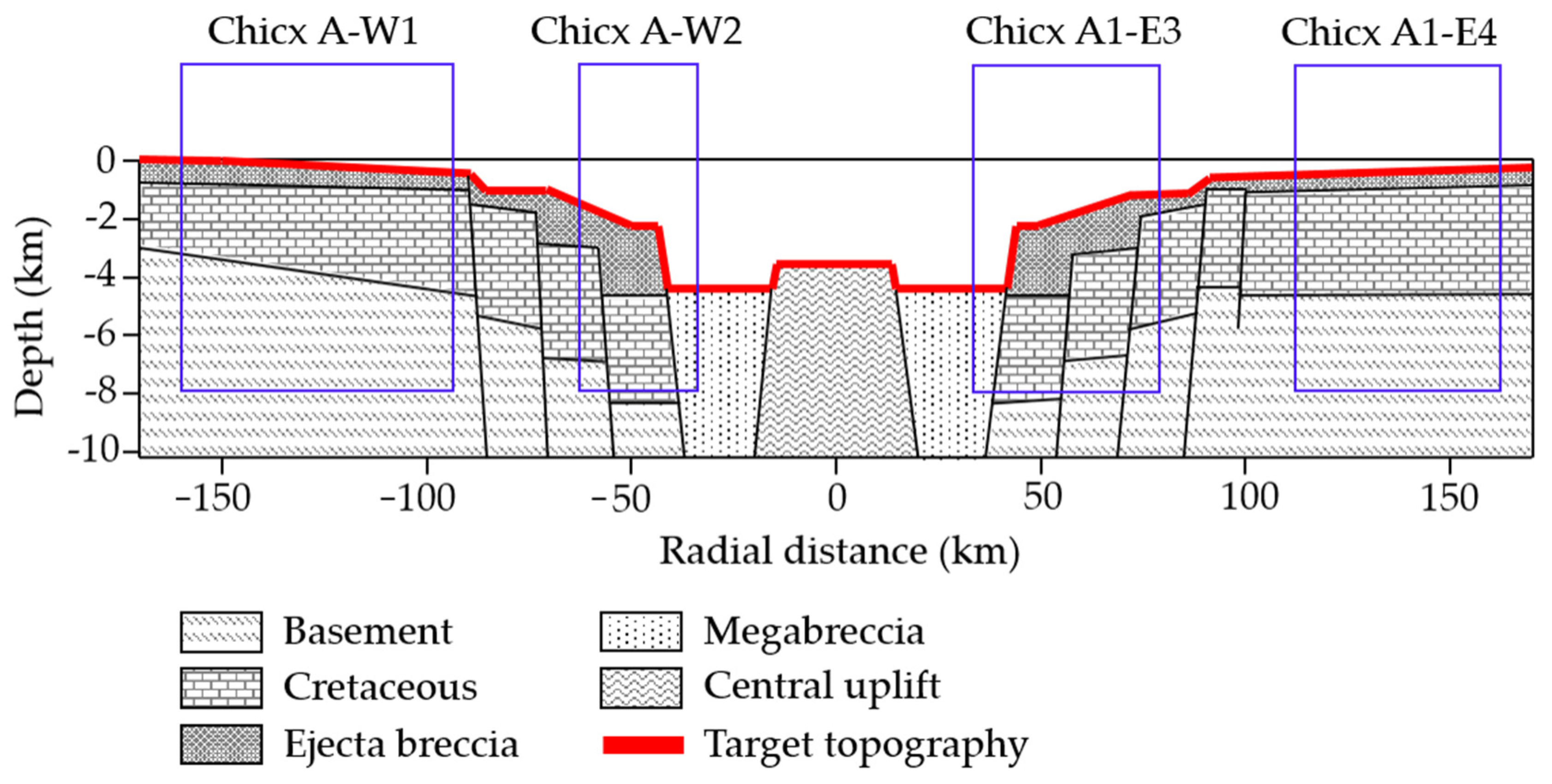
2. Characteristics of Chicxulub Crater
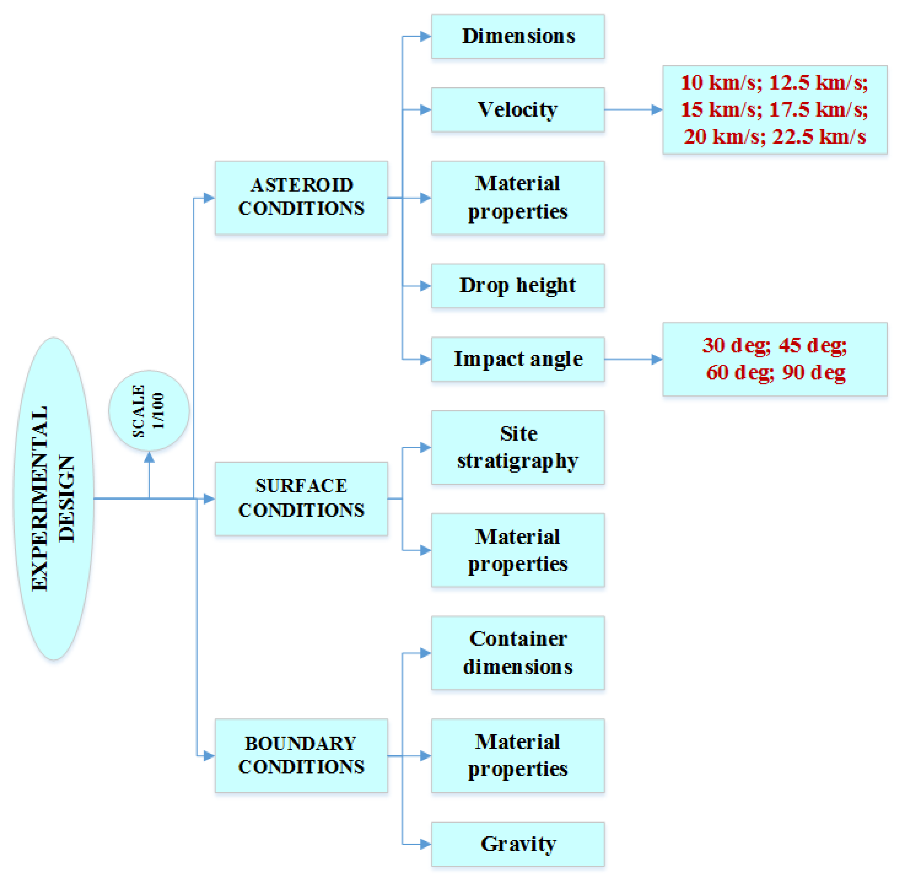
Since its discovery as part of Mexico’s oil exploration program, the Chicxulub crater (located in the Yucatan carbonate platform, south of the Gulf of Mexico) has undergone numerous geophysical studies and drilling programs. These have produced information describing the crater formation process, the climatic and environmental effects of the impact, the global distribution of the Iridium-rich clay layer which marks the K/Pg boundary, and the link between the Chicxulub impact and the mass extinction of the dinosaurs [1]. The Chicxulub crater is classified as a complex crater, consisting of three rings with a central peak of about 40 km, two lower rings at about 70 km and 120 km which serve as the inner and outer limits of the transient crater wall, and a basin outer rim of about 200 km in diameter [1]. The estimated size of the asteroid is about 10 ± 4 km in diameter, with an estimated impact velocity of about 15–22 km/s [1].
The crater formation process consists of several stages [5,6,7,8,9,10,11]. The first stage is called the compression stage, wherein the projectile hits the planet surface, creating shock waves through the conversion of kinetic energy. Part of the shock waves transmitting to the ground is reflected back into the asteroid as tensional waves or as a rarefaction that decomposes, melts, and vaporizes the subject. The following stage is called the excavation stage, which develops the asteroid melt lining in the expanding transient cavity and creates an outward ejecta blanket from the opening crater. After that, the modification stage steps in, as the oversteepened walls of transient crater or ejecta fall back into the cavity to form a deposit of mixed breccia. The final simple crater type thus forms, a bowl-shaped depression made of mixed breccia and impact melt bodies. Complex craters are formed due to complex interactions between shock wave effects, gravity, and the strength and structure of the target rocks, resulting in the formation of a central uplift and one or more depressed rings toward the crater ring [1,2,3,4,5,6,7,8,9,10,11].
Different drilling programs have been conducted at the crater site to obtain information on the subsurface stratigraphy, the structure and material of the underlying sediments for further study of shock effects, and the lithologies and deep layer components. Such programs include the International Ocean Discovery Program (IODP), the Petroleos Mexicanos (PEMEX) program, the National University of Mexico (UNAM) drilling program, the Chicxulub Scientific Drilling Project (CSDP), and the UNAM drilling program in collaboration with the Federal Commission of Electricity (CFE) [3,11]. Locations of all previous geophysical explorations and drilling studies are presented in the IODP Expedition 364 report [42]. Drilling cores were collected at the boreholes and subjected to different tests and scanning to classify the materials and obtain their physical properties. Based on the information acquired from these geologic and geophysical site investigations, including core samples, the corresponding Chicxulub crater structure was drawn with respect to drilling locations, as is shown in Figure 1.
Figure 1 shows the crater’s cross-sectional profile after the asteroid impact, and before any filling sedimentation started (marked with the red line). This profile was used as the target structure benchmark for the model used in this study. Notice that the proposed DEM modeling approach used in this study allows for a direct comparison with the crater’s target profile, creating an opportunity to highlight the differences between previous continuum and discrete modeling approaches.

3. Methodology

Numerical simulations of the asteroid impact were performed based on an experimental design including the considerations outlined below. The models’ scaling ratio of the whole system size was set to 1/100 to reduce computational cost in numerical simulations. To maintain energetic consistency in the scaling, the velocity of the asteroid was reduced 10 times to scale down kinetic energy by a factor of 100. The experimental design chart for asteroid simulations is presented in Figure 2. The model is made up of three parts: asteroid conditions, ground surface conditions, and the boundary conditions. The asteroid conditions include the asteroid size, asteroid material properties, asteroid drop height, impact angle, and asteroid velocity. The surface conditions include the site stratigraphy and material properties. The boundary conditions include the model’s ‘container’ dimensions, container properties, and gravity.
For this study, only the impact angle and the asteroid velocity were defined as control variables, to follow the numerical experiment set by Collins et al. [19], who considered four different impact angles (90°, 60°, 45° and 30°) and two impact velocities (12 and 20 km/s), while keeping the remaining variables constant. These values of velocity and impact angle are also consistent with the findings from craters caused by oblique impacts, such as those explored by Pierazzo and Melosh [13]. The dimension of the asteroid was kept constant at a diameter of 10 km [43] and subjected to 1/10 downscaling to maintain consistent reduction ratio of 1/100 of the kinetic energy across the entire downscaled system. The drop height was not considered as this study assumed that the asteroid had reached terminal velocity before impact (i.e., the asteroid’s velocity is not a function of the drop height).

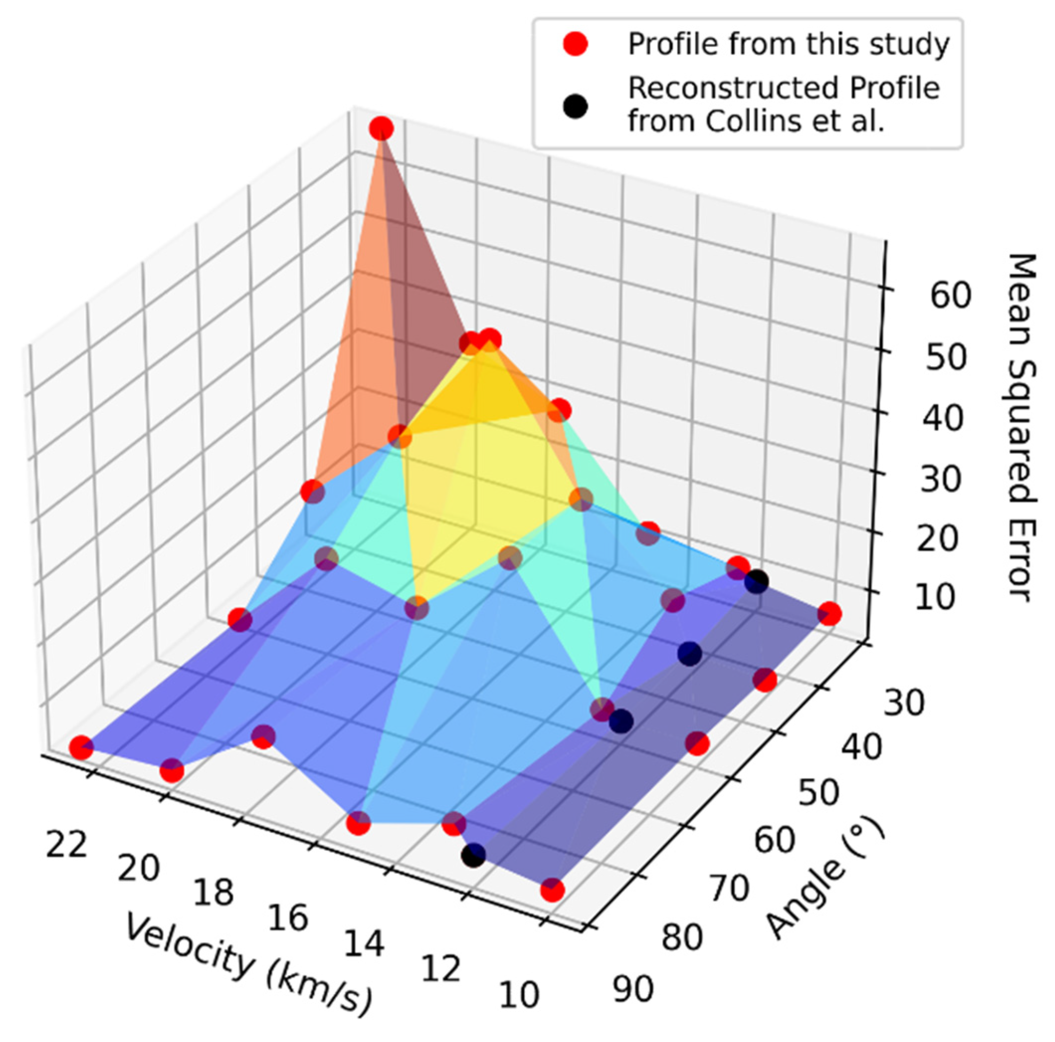
Profile Reconstruction and Comparison Methodology

Results from Collins et al. [19] illustrated the postimpact surface topography after impact with the asteroid moving in an easterly to northerly direction. Recent findings from Collins et al. [18] claimed that the Chicxulub asteroid most likely came in the direction of northeast moving southwest, which was in contrast with a previous study by Hildebrand et al. [44]. Based on the locations of the three centers (i.e., mantle uplift center, crater center, and peak ring center), results from Collins et al. [19], wherein the authors presented their surface topography for impact direction from right to left, were reoriented to match the newly claimed asteroid impact direction coming from northeast to southwest, and then rescaled, with the peak ring center and its annular boundary as the reference points. Then, the reoriented postimpact topography from Collins et al. [19] was superimposed on the aerial map in Figure 3, and both regions of uplift and depression were marked with the red and blue boundaries, respectively. A straight line representing the ‘Chicx-A/A1′ cross section is also shown in Figure 3, which extends to about 340 km.
An approximate reconstruction of the surface topology of Collins et al. [19] was conducted by extracting the pixel values in the image and matching them with the corresponding scale. The portion of ‘Chicx-A/A1′ that crossed the surface topography plots in Figure 3 was approximately 260 km long. The reconstructed profile was offset by about 20 km to the right, so as to better compare with the benchmark profile ‘Chicx-A/A1′. Comparisons across all the crater stratigraphy are discussed in the following sections. Notice that the asteroid impact direction set up in this study was originally set from the left direction moving to the right in a 2D plane (there was no particular reason to select the impact orientation at the time the proposed DEM model was formulated). Therefore, to be able to compare the DEM results of this study with Collins et al. [19], the DEM simulation results were symmetrically mirrored to match Collins et al. [18] asteroid’s impact from right to left.

4. DEM Model

The DEM model impact configuration is shown in Figure 4, showing the two control variables: impact velocity (v) and impact angle (β). The asteroid diameter was scaled down to 100 m, and consisted of bonded particles of 10 m diameter. For all case studies, the vertical drop height of the asteroid remained constant, at 500 m above the ground’s surface. The material densities of both the ground and asteroid were assumed to be equal, at 3000 kg/m3. The model was composed of nine different layers with increasing particle size from the surface to the container baseline, corresponding to the observed stratigraphy (i.e., ranging from 5 m to 40 m in diameter). Table 1 includes each layer depth and its corresponding particle size. Notice that the increase in particle size was considered to reduce computational costs, as well as to reflect the physical aspect of basement rocks and mantle layers. The first three layers had the properties of a weak sedimentary limestone layer, while the rest had properties of hard granite rocks. The stratigraphy configuration was obtained by reproducing a sedimentary process under gravity. The asteroid had identical properties to the sedimentary limestone layer. The model’s particle container size used in the numerical simulation was set to 4 km by 2 km after downscaling the actual stratigraphy, and the Earth’s gravitational force of 9.81 m/s2 was considered throughout the simulations.

4.1. Constitutive Model

A ‘linear parallel bond contact model’ was used to resemble the rock mechanic behavior for all stratigraphy layers. The use of the bonded-particle models in rock mechanics studies has been popular practice, according to Potyondy’s study [45]. The PFC manual [46] shows that parallel bonding provides the mechanical behavior of a cementlike material gluing two particles of the same material together. The bond component acts like a set of elastic springs to induce a constant normal and shear stiffness, evenly distributed force and moment, across the contact plane. As the stresses applying on the particles exceed the bond strength, the contact bond breaks and is removed from the model. The contact model then becomes a ‘simple linear contact model’ [46]. Values of the limestone parameters were adopted from Ledgerwood’s study on high rock pressure conditions [32]. The model parameters used in this study were also calibrated, and the calibration results showed agreement with the reference. The contact model parameters used in the simulations are listed in Table 2. Material properties of the asteroid in the simulation were assigned from the K–Pg boundary in the stratigraphy [47,48] between Cretaceous and Paleogene rock layers. Studies on samples from the breccia and melt rock units in the Chicxulub crater have also been considered [49,50]. Evidence from geochemical and isotopic studies [48,49,50] suggests that the Chicxulub impactor was made up of carbonaceous chondrite, due to the discovery of extraterrestrial matter composed of carbonaceous chondrite in the boundary layer. Thus, the material of the asteroid is assumed to be composed of the same material where the K–Pg boundary in the rock layers lies.

4.2. Boundary Conditions

A far-field infinite boundary condition was set up in the model by assigning the wall component’s normal and shear damping ratio at 1.0, which meant the entire energy of the particles would be absorbed when they were in contact with the walls. To validate the absorbing aspect of the boundary, a simple test was set up where a rolling particle hit a chain of five contiguous particles placed at the corner of the model’s container, and the postimpact velocities of the first and the last particles of the chain were recorded and shown in Figure 5. The velocity of the particle at the corner (1) showed that it quickly converged to zero after the impact, while the particle initially in contact with the rolling ball (5) shows an immediate velocity increase which dissipated post impact. The force reflection effect at the model’s container boundary was not observed, thus indicating a full energy dissipation at the model’s boundary.

4.3. Control (Measurement) Circles

A set of control (measurement) circles were defined along the center line of the model’s container and along the container’s boundaries, to trace the mechanical response during and after the asteroid’s impact. This allowed us to track horizontal and lateral stresses, in addition to the average interparticle contacts per particle (i.e., coordinate number). The radiuses of the control circles along the center line and the boundaries were 200 m and 20 m, respectively, as this yielded adequate measurement resolution. Figure 6 shows the locations of the measurement circles on the model’s container centerline, and along its vertical and horizontal wall boundaries.

5. Simulation Results

A set of numerical simulations of the asteroid’s impact were performed based on the proposed experimental design (Figure 2), with varying impact angles and asteroid velocities. Each simulation was run until the surface particles’ velocity was less than 1 m/s or until 2 million calculation cycles were completed to secure a postimpact pseudostatic condition. Results of the simulations are presented below. Short videos of the asteroid impact simulations for each numerical experiment can be found at the Stochastic Geomechanics Laboratory SGL YouTube channel: https://www.youtube.com/playlist?list=PLdR9gOvj-F2gHCPmzJq0Kz_RsC5AiFHqp (accessed on 2 May 2023).

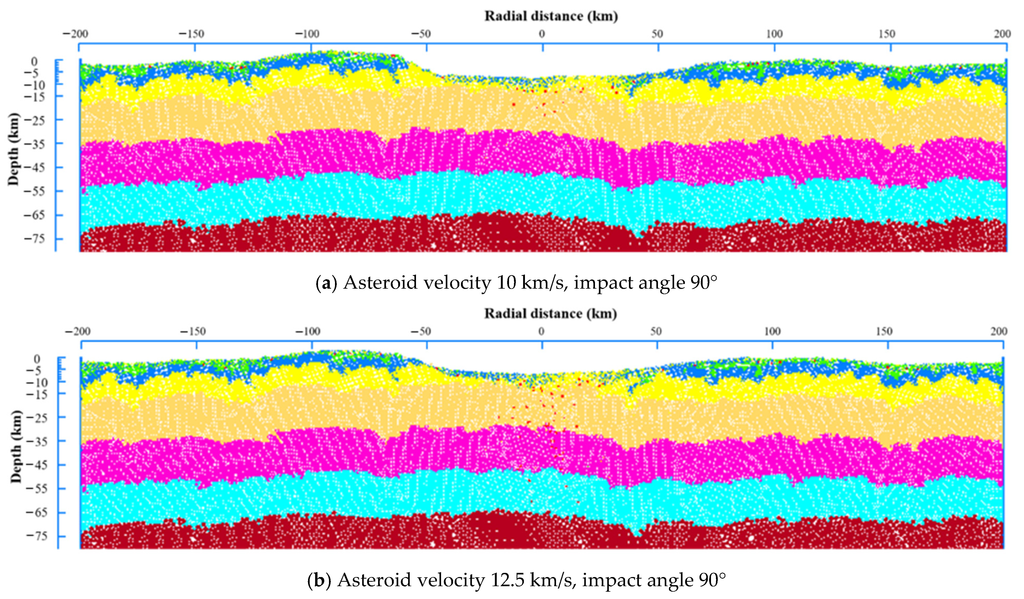
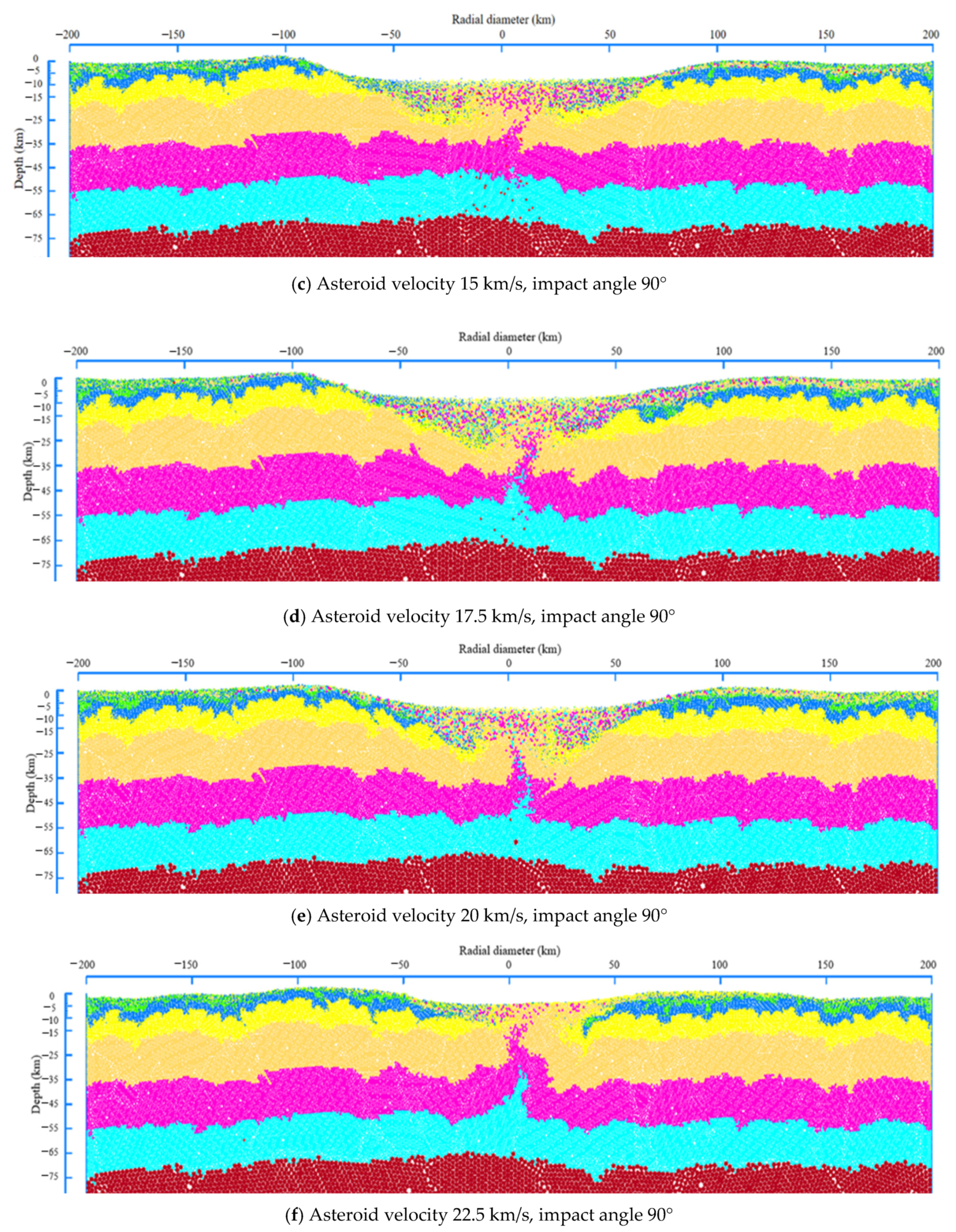
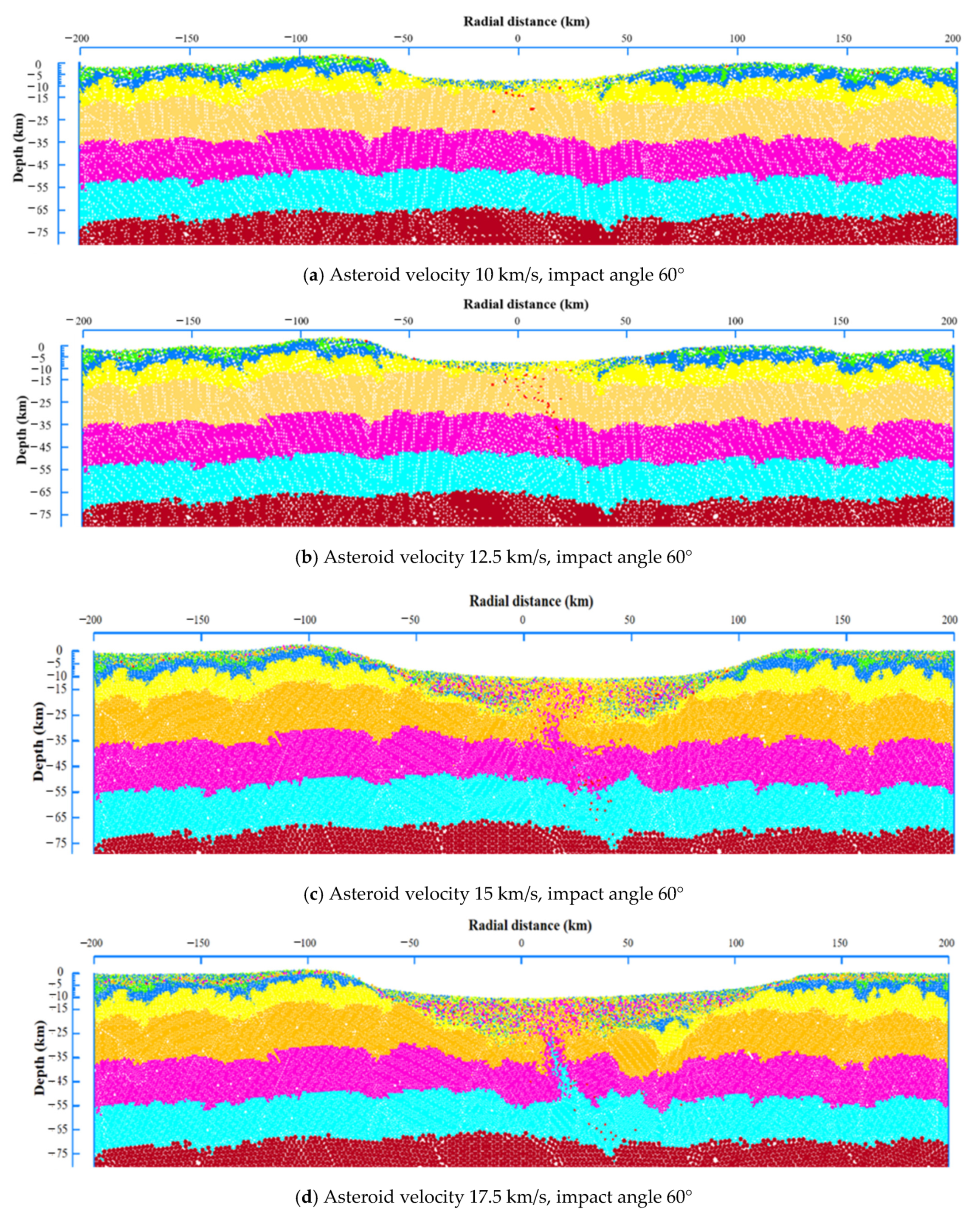
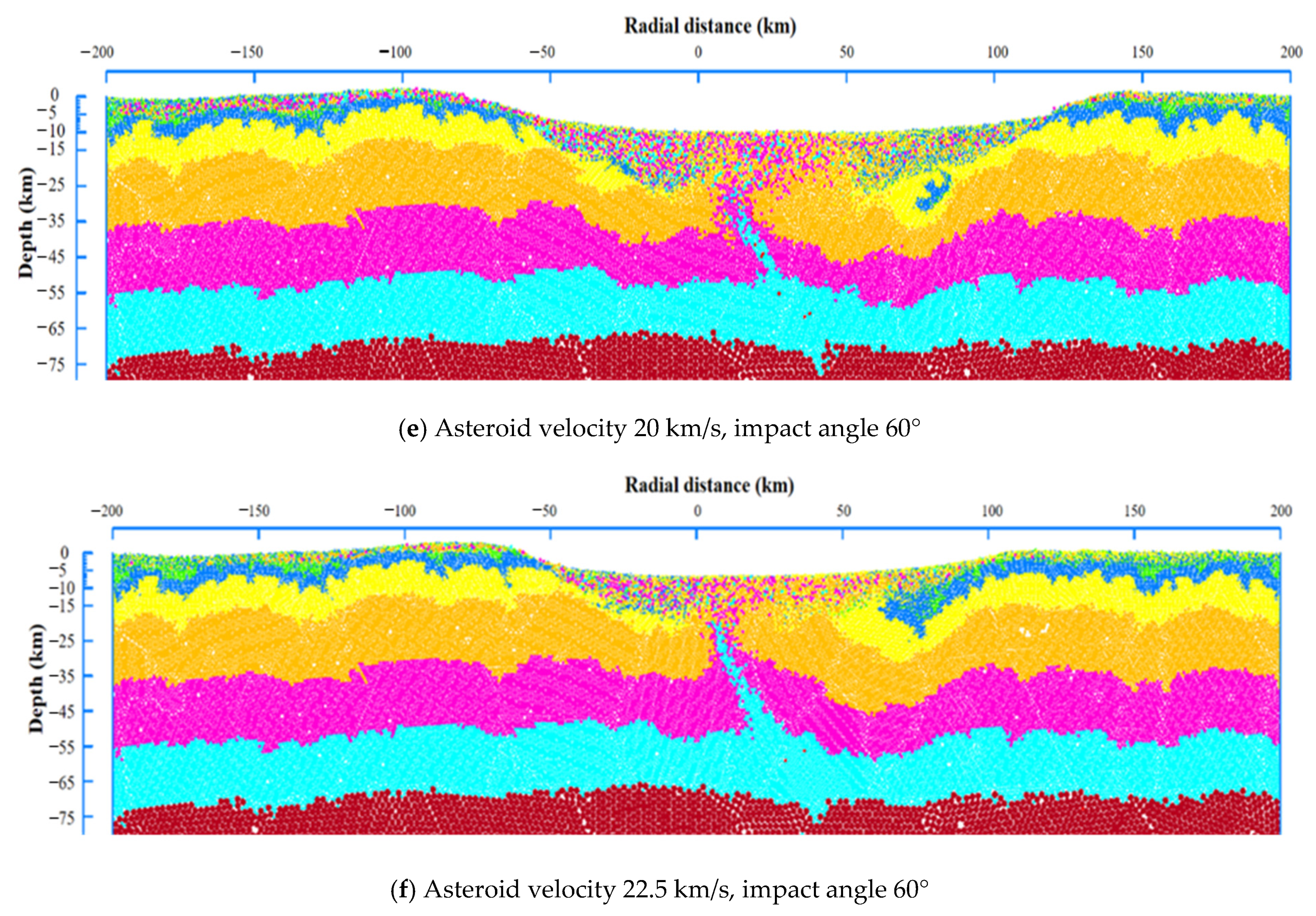
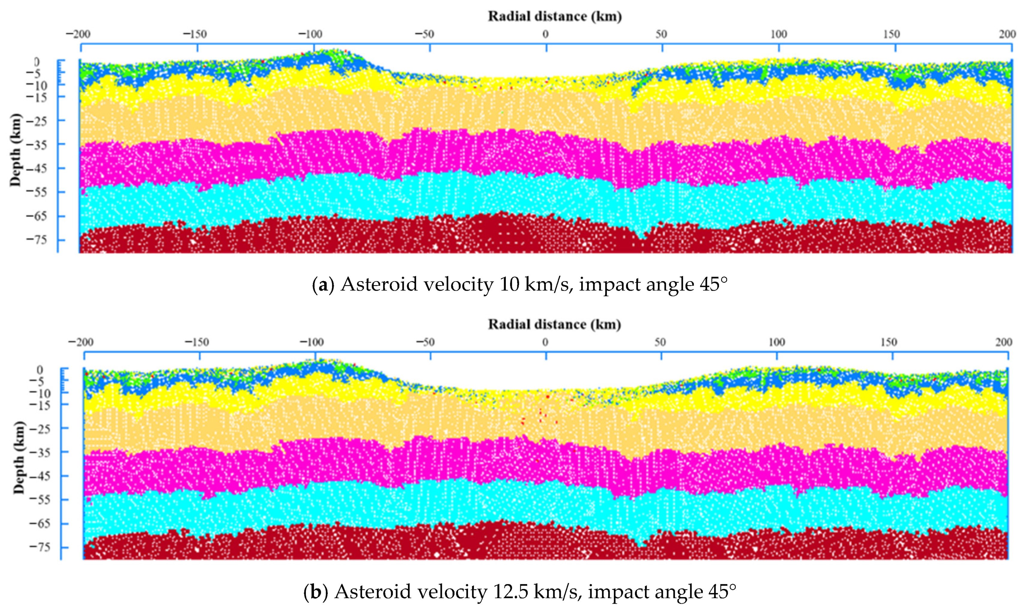
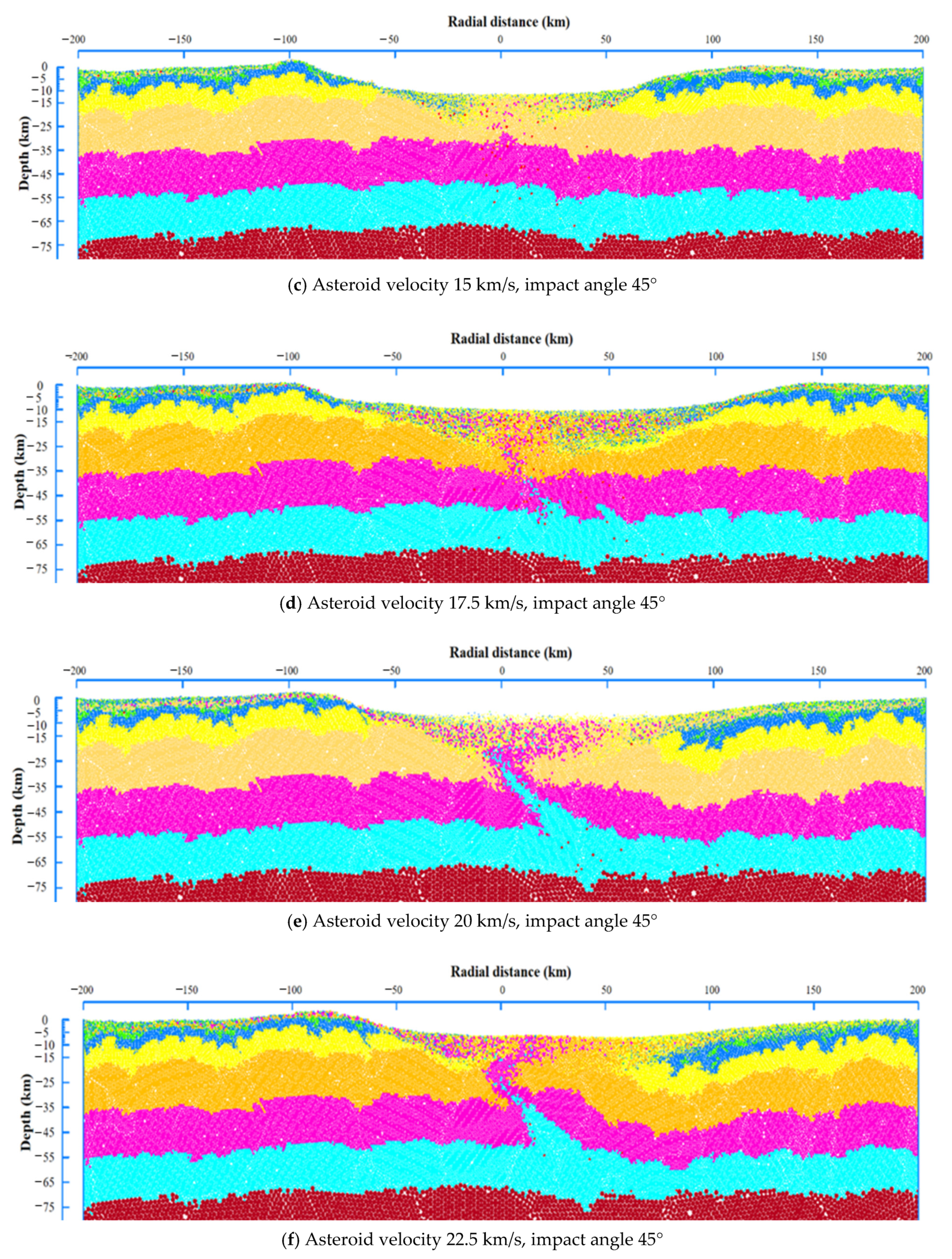
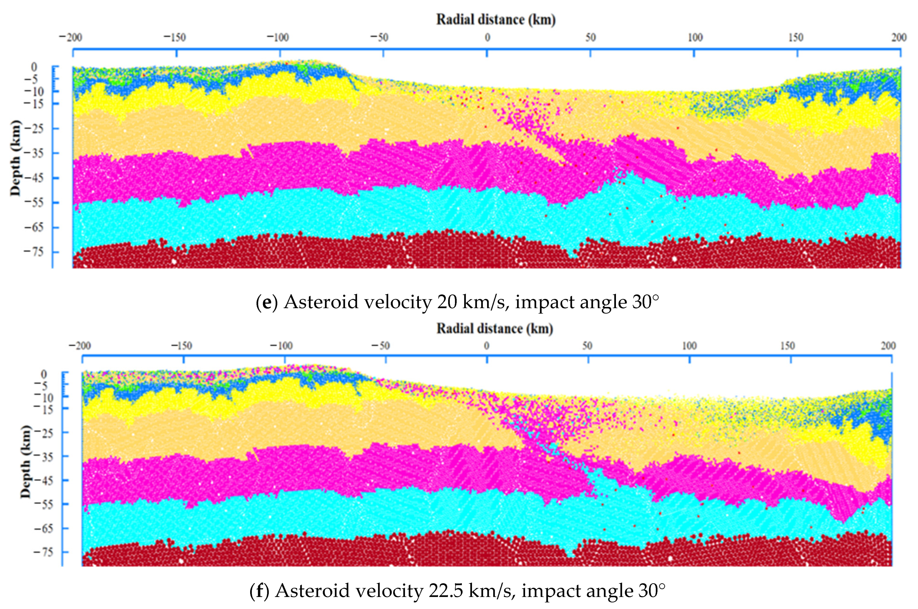
5.1. Crater Surface Topography

Surface topography of each impact case was compared with the real Chicxulub crater surface topography obtained from geophysical and geological drilling explorations [2,3,4,5]. Figure 7 shows the topographic configurations of each set of simulations at different impact angles and at different impact velocities. These were then compared with the target topographic model. This figure shows that the crater diameter for an impact angle of 30° showed the most significant increase and variation of all impact angles, and that the rise of the crater rims was also higher for nonvertical impacts. Also, it was observed that simulations with an impact angle of 90° yielded a better match to the target site topography. A discussion on the quantitative differences between simulations and the target topography of the crater is presented in the following section.
The DEM simulations suggested that the inclined impacts provided more uplift in the crater rim in the upward direction than in the downward direction. These findings were counter to those of the previous study by Collin’s et al. [18]. Such difference might be caused by the difference in the mechanical premises between DEM and hydrocode-based modeling methods. Determining the impact angle and trajectory has been investigated from field observations and numerical simulations [13,18,19,51]. Crater-forming impacts involve high energy release with high temperatures and pressures across short time scales. Their structural and morphological characteristics depend on several interconnected factors, including the impact dynamics, target, and bolide characteristics and formations mechanisms, all of which are reflected in the wide range of craters observed in planetary bodies [51,52]. Note that Figure 7 also includes the reconstructed profiles from Collins et al. [19], which showed that their reconstructed profiles were consistently above the actual postimpact topography observed in the field. When compared to the DEM simulation, the 3D iSALE simulation managed to reproduce complex crater formation, characterized by the uplift formation in the center. From all the DEM simulations with varying impact velocities and angles, the DEM model consistently reproduced simple crater formation (bowl-like in shape). The target postimpact topography has a slight uplift in the center of the crater, and the DEM model had not captured such an effect. One likely contributing factor leading to such differences could be the scale of the proposed numerical experiment; DEM modeling of impacts is suitable for capturing micromechanical behavior in a smaller-scale numerical experiment, but due to the scale of the asteroid impact, the model did not seem to show any plastic behavior, despite the addition of bonding between the particles, as shown in Table 2. Another possibility for such difference may be the infinite boundary condition, which does not include a rebound effect from the model boundaries, limiting the potential development of the uplift formation in the center of the crater.
Due to the random nature of the particle deposition induced during the particle generation algorithm [42], the stratigraphy of the DEM models prior to the impact showed layer horizons which were not perfectly flat. In contrast, typical known continuum-based models set their model’s stratigraphy showing layer horizons where are completely flat (e.g., Collins et al. [18]). Differences in the modeling approaches led consequently to two distinct behaviors, where results from the continuum-based model achieved close to perfect crater topographic symmetry on the 90° asteroid’s impact inclination, while DEM show a less symmetrical surface topography (Figure 7).
The final crater vertical cross-section configurations for each impact simulation are presented in Appendix A (Figure A1, Figure A2, Figure A3 and Figure A4). The models showed that the asteroid velocity plays an essential role on the final definition of the crater topography. Notice that the uplifting effect was more visible as the asteroid impact velocity increased. The shearing effect in the rock layers due to different impact angles also depended on the asteroid impact velocity. The terrace zone and crater rim effects were also observed in the resting crater configuration. The distribution of the middle rock layer (pink particles) flew out after impact, and then concentrated near the surface, showing a clear internal uplifting process. This effect was more noticeable for the case of smaller impact angles when combined with high impact velocities.

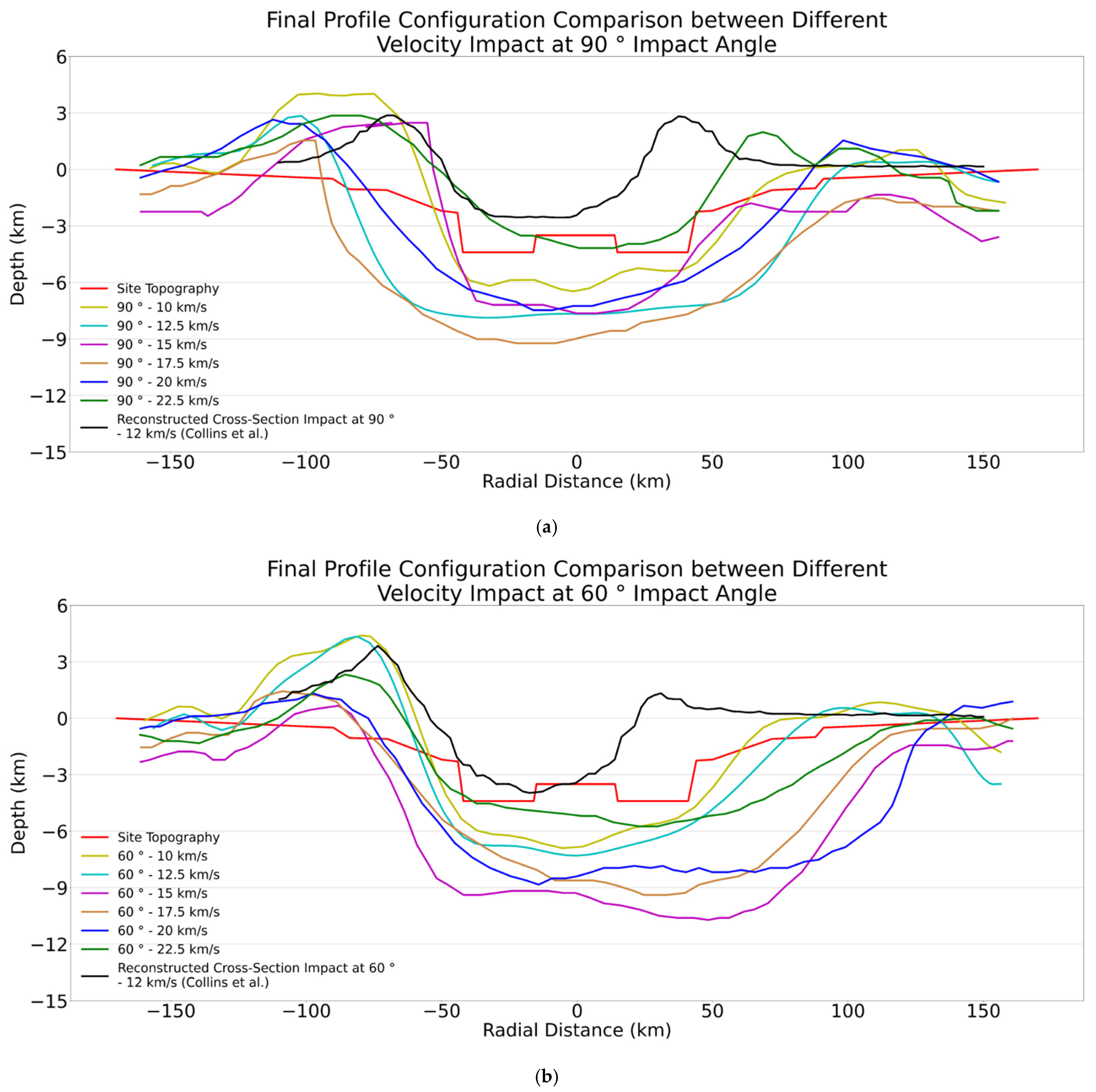
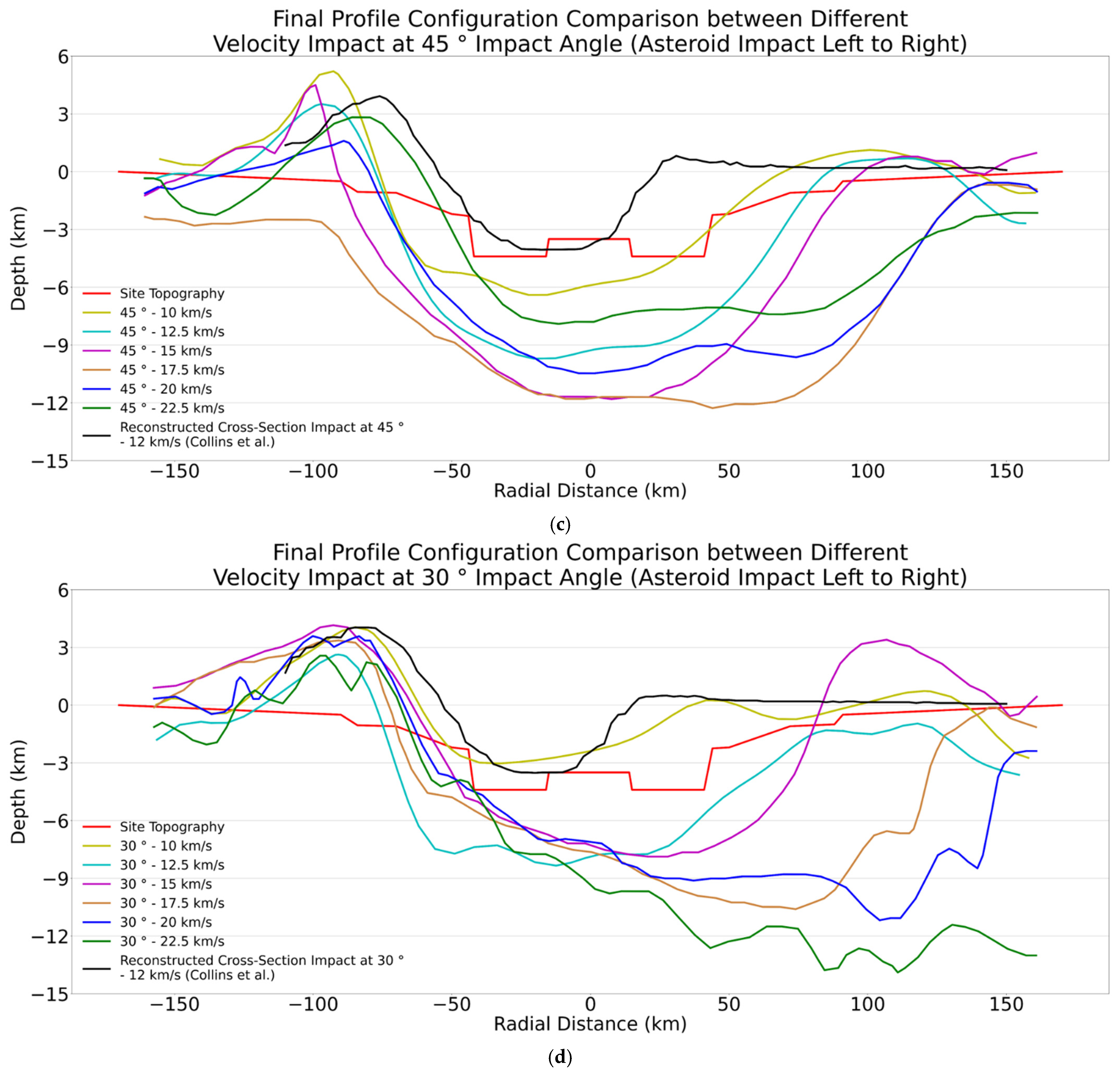
5.2. Simulated vs. Target Profile Analysis

A quantitative analysis was conducted to compare all topographic profiles from the DEM model simulations with respect to the target surface topography. A simple mean square error (MSE) criterion was used to evaluate how close the overall simulated profile was to the target profile ‘Chicx-A/A1′ (the red profile in Figure 7). The range of radial distance that was used in the MSE computation was from −110 km to 150 km, since this was the available range for the profile reconstruction from Collins et al. [19] (Figure 7). The MSE is calculated using:
M S E = 1 n i = 1 n Y t a r g e t , i Y s i m u l a t e d   p r o f i l e , i 2
Figure 8 summarizes the MSE values of the simulated topographic profiles produced in this study and by Collins et al. [19], compared against the target topography (Figure 1). From this figure, it was observed from the DEM simulations that, at low asteroid’s impact velocities (from close to 10 km/s to 12.5 km/s), any impact angle seemed to yield the lowest MSE values. On the other hand, the simulated profile with a low impact angle 30° and a high velocity 22.5 km/s showed the highest MSE value. Moreover, the impact angle of 90° paired with any velocity values seems to produce the closest match to the target topography. On the other hand, results from Collins et al. [19] showed little MSE variation at velocities of 12.5 km/s or lower, regardless of impact angle.

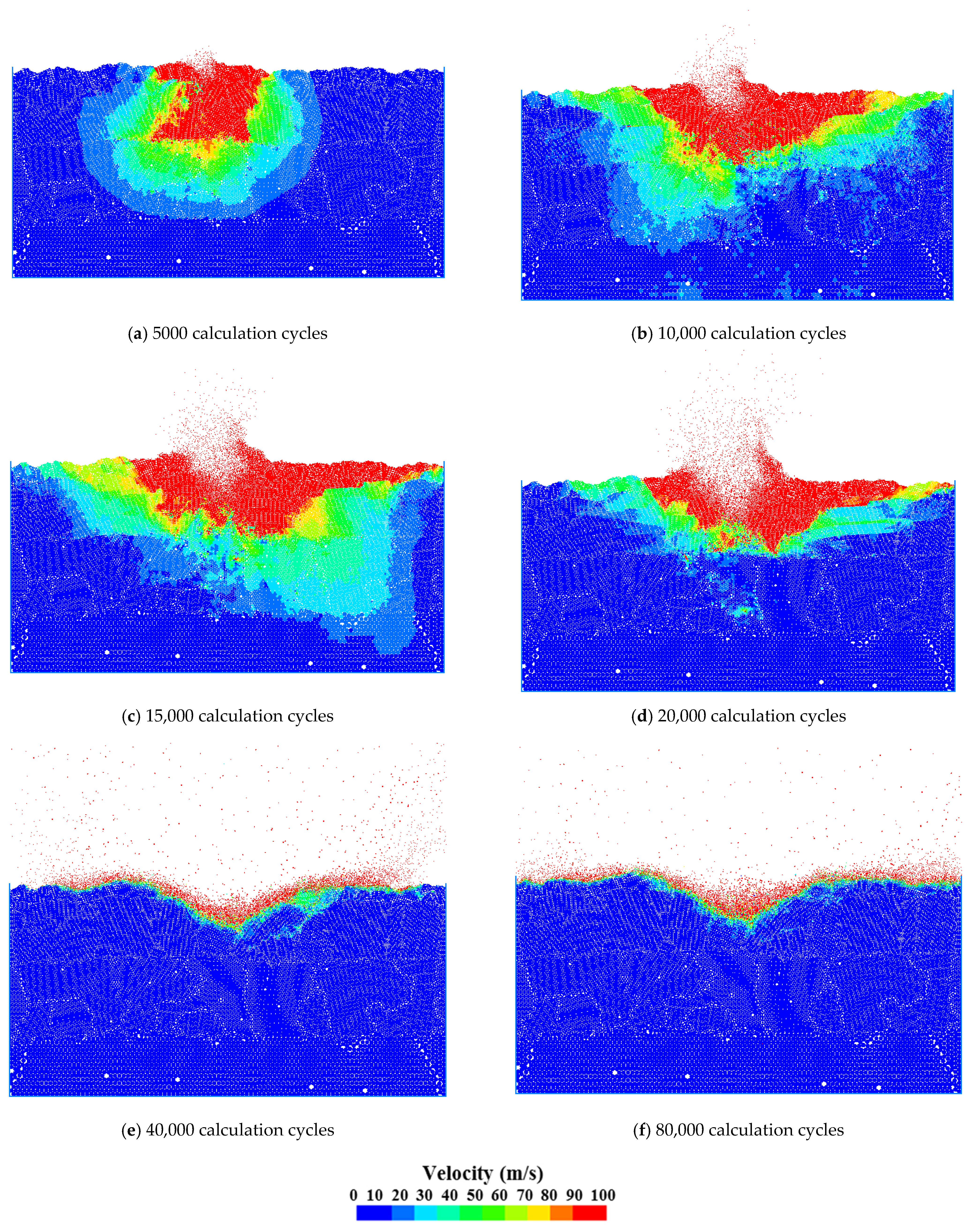
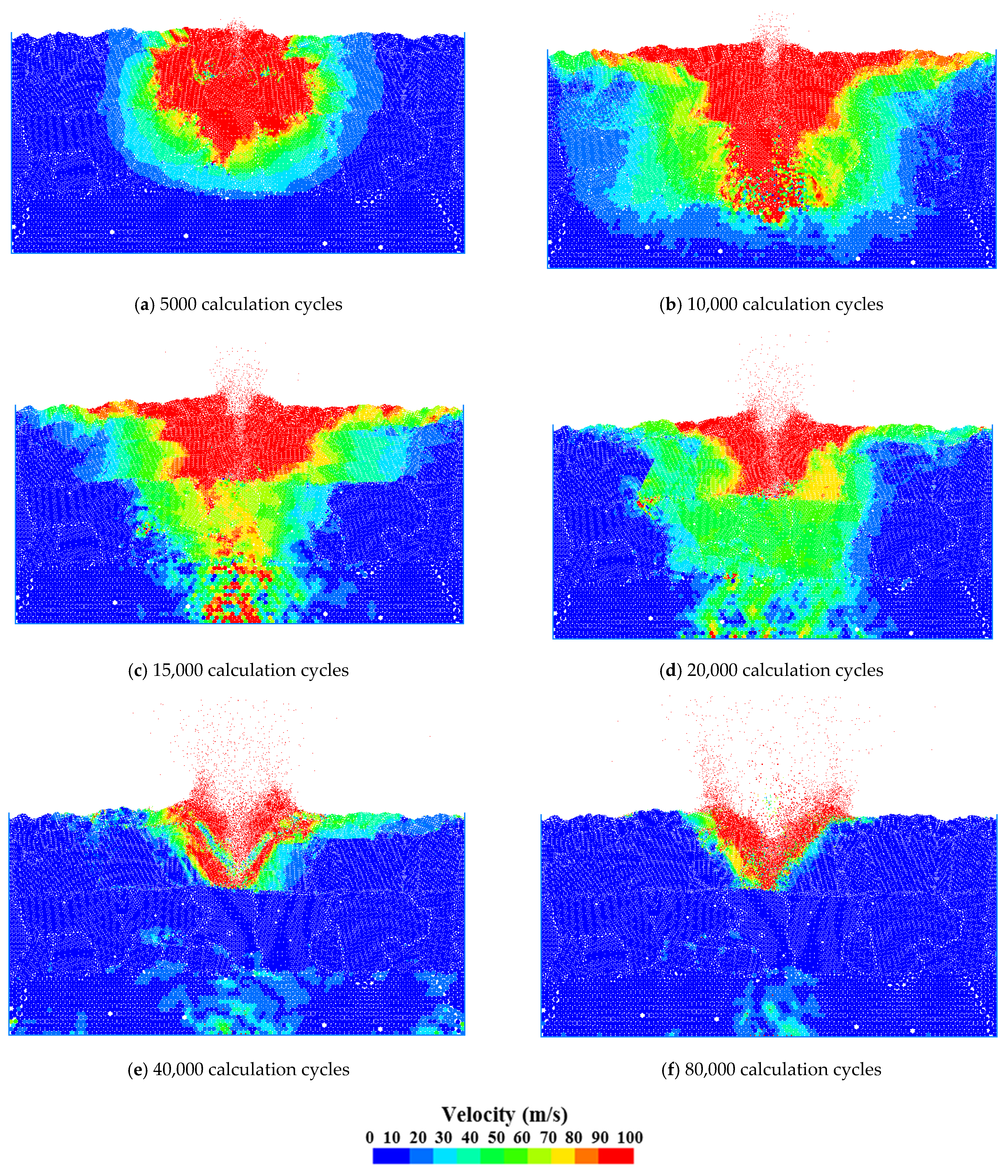
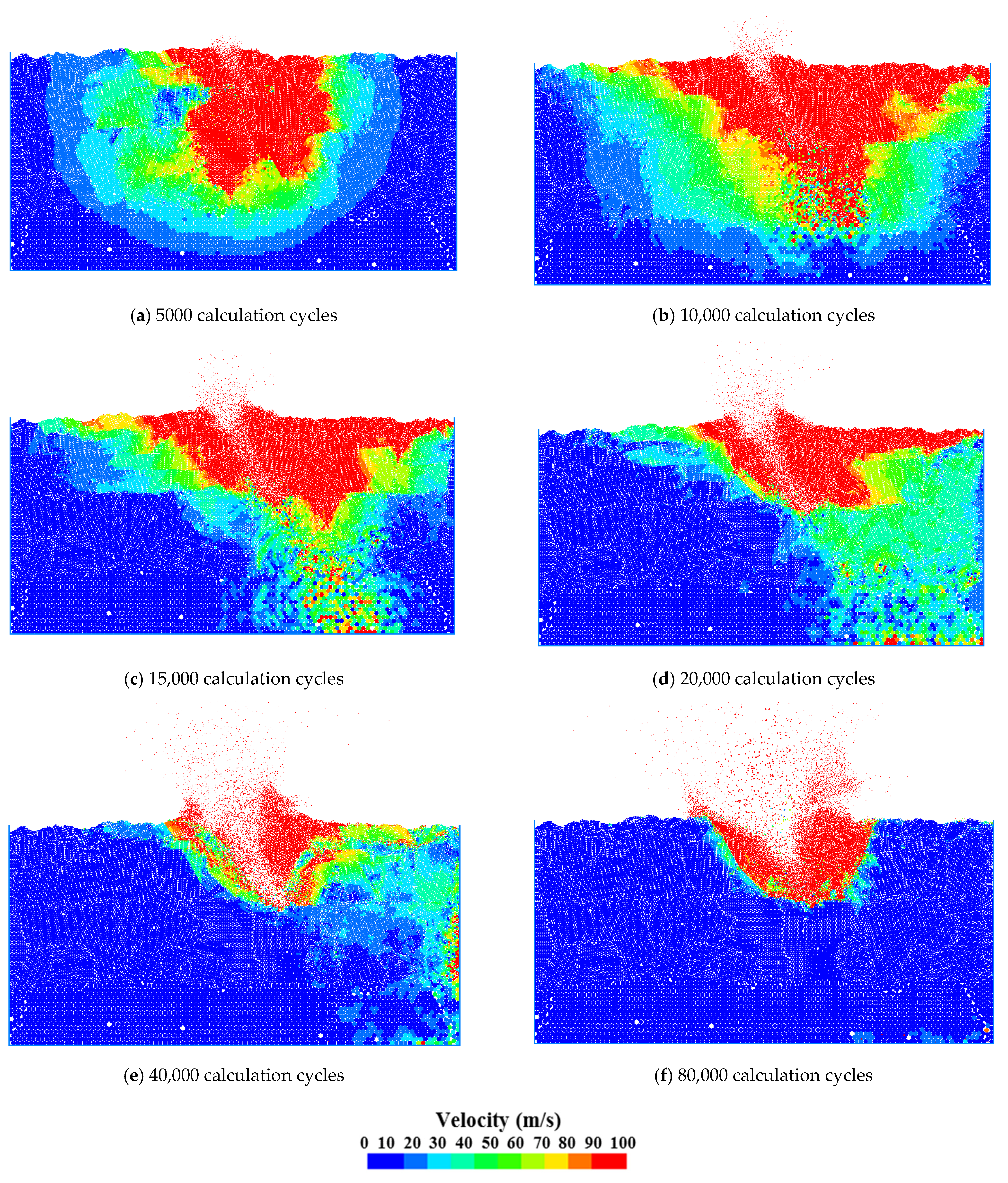
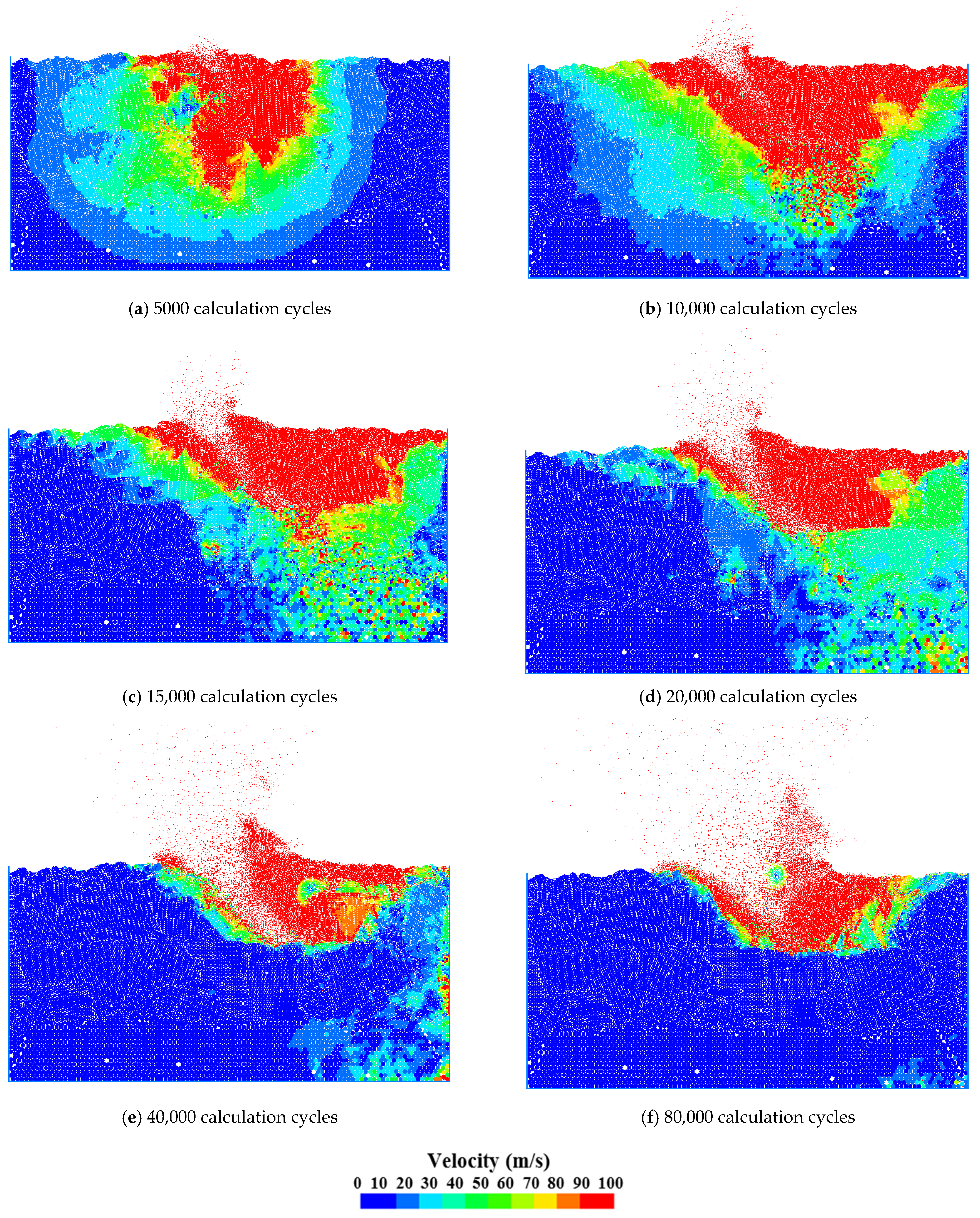
5.3. Velocity Fields

Velocity fields were obtained for each combination throughout the impact and crater formation process. The main motivation for tracing the velocity fields response was to see how the impact-induced velocity travels through the surface immediately after the asteorid impact. Figure A5, Figure A6, Figure A7, Figure A8, Figure A9, Figure A10, Figure A11 and Figure A12 in the Appendix A show the velocity of particles in the ground captured at 5000, 10,000, 15,000, 20,000, 40,000, and 80,000 calculation cycles (which is equivalent to 1 s, 2 s, 3 s, 4 s, 8 s, and 16 s after impact, respectively) by taking the average timestep of 2.0 × 10⁻⁴ s/calculation cycle. Figure A5, Figure A6, Figure A7 and Figure A8 show simulations from the asteroid impact at 90°, 60°, 45°, 30° inclinations at 15 km/s impact velocity, and Figure A9, Figure A10, Figure A11 and Figure A12 show simulations at 90°, 60°, 45°, 30° inclinations and at 22.5 km/s. A comparative analysis across these two sets of simulations showed the relevance of the asteroid’s impact velocity and inclination, and its nonlinear association as depicted in Figure 8, which further provided a better understanding of the likely phenomenological behavior of the asteroid impact and the crater formation process.

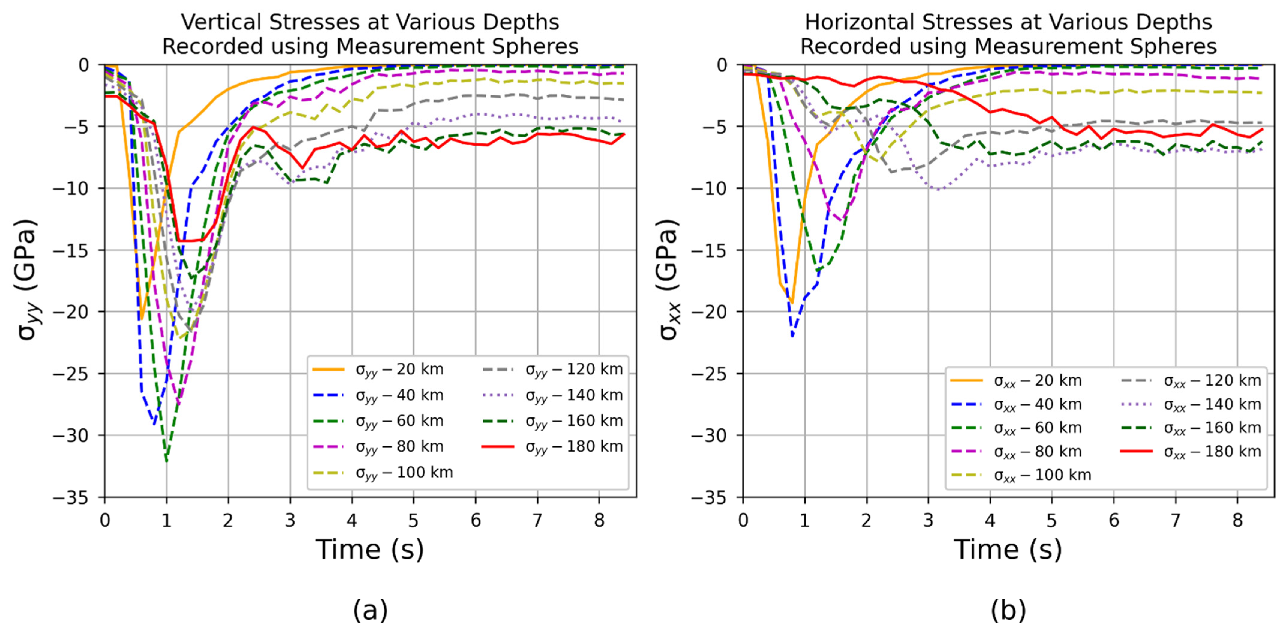
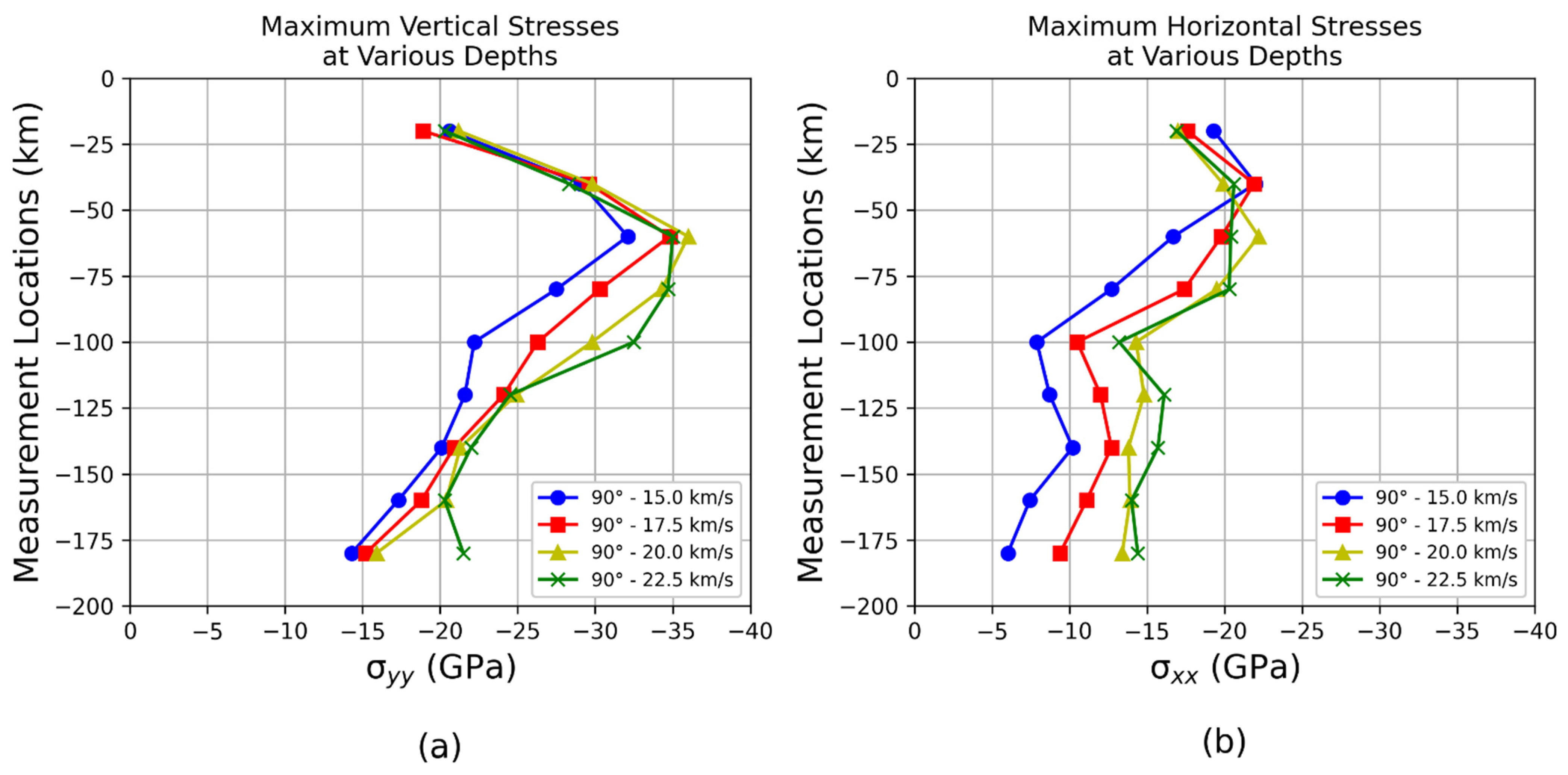
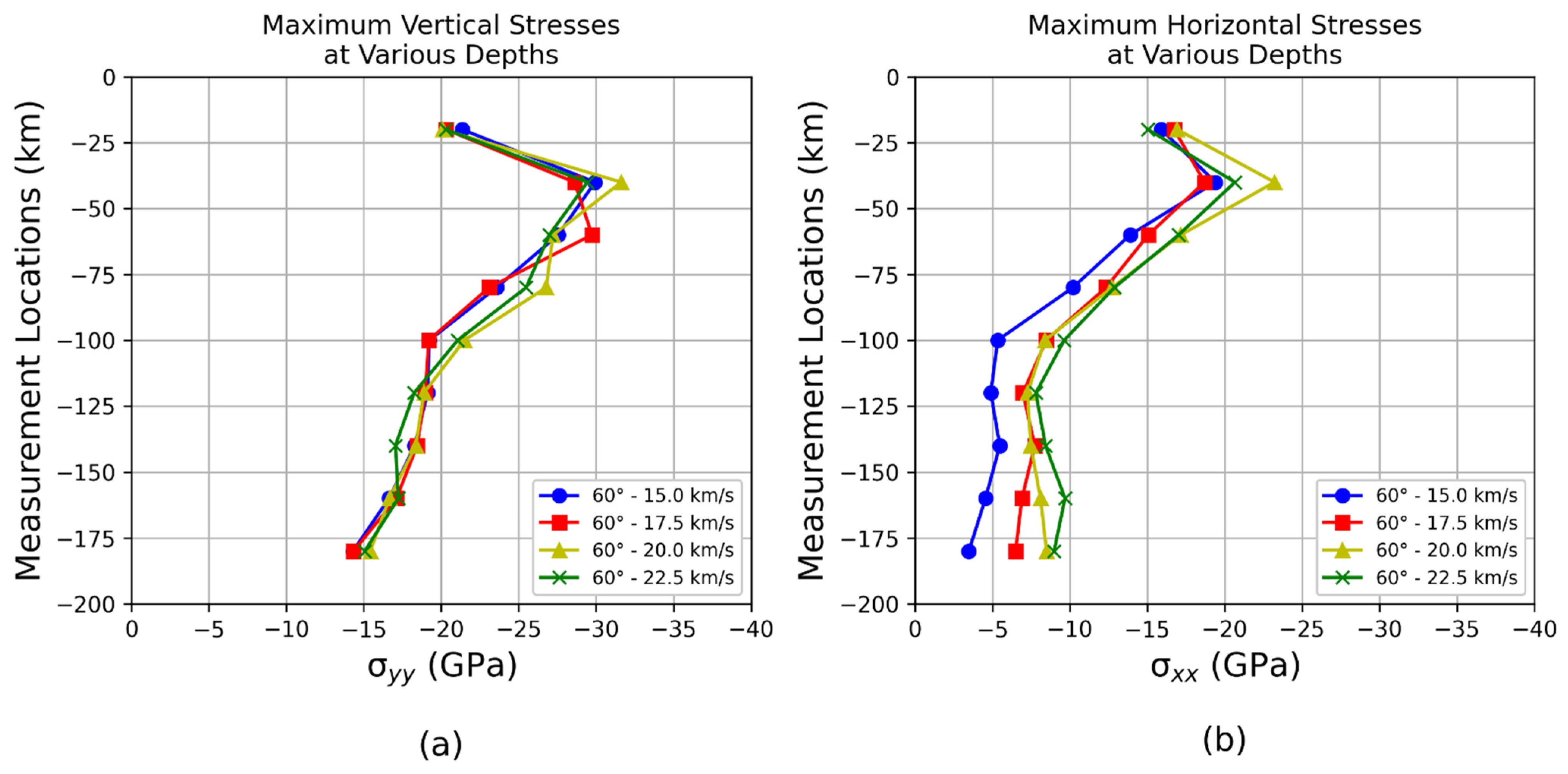
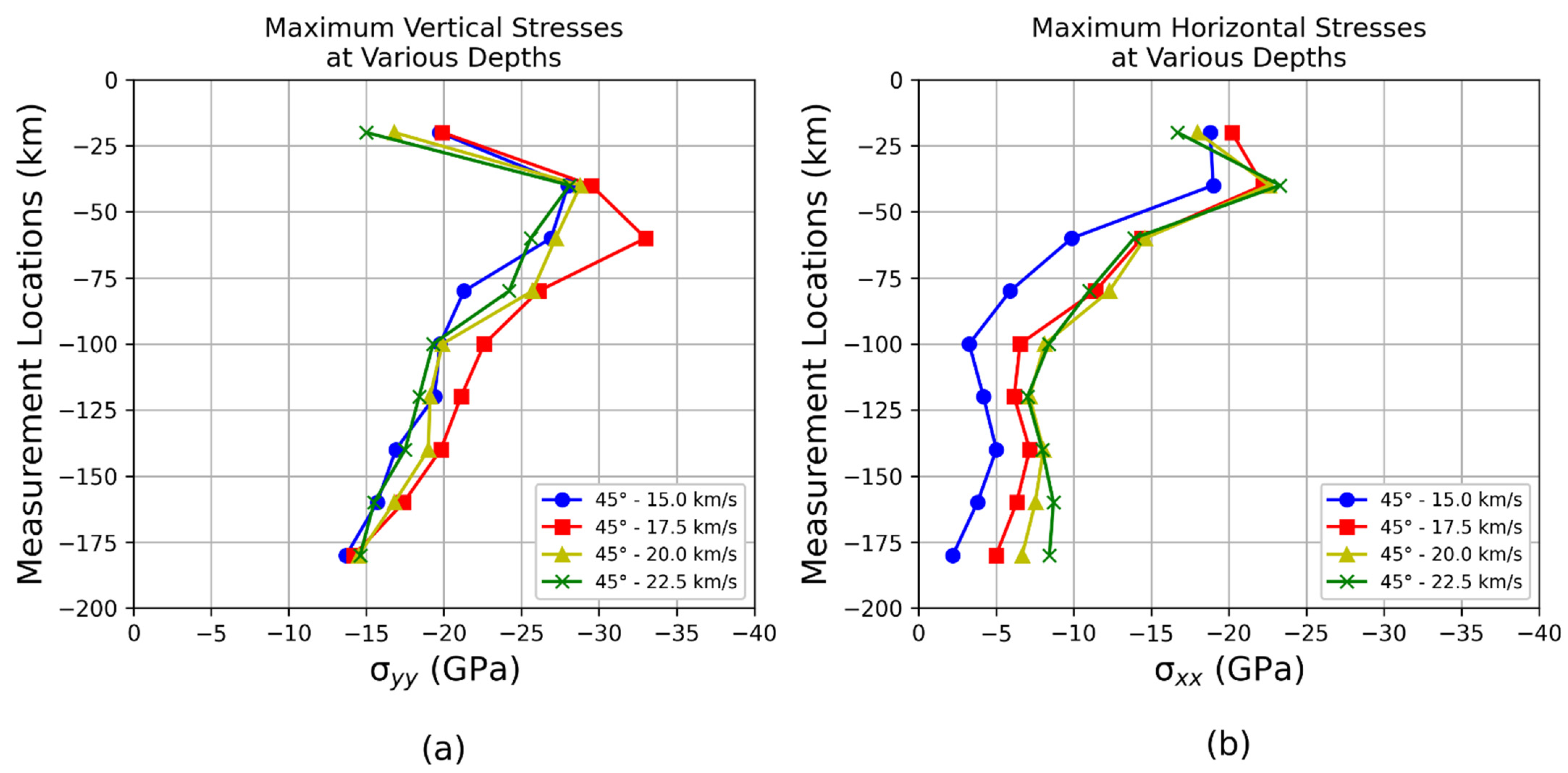
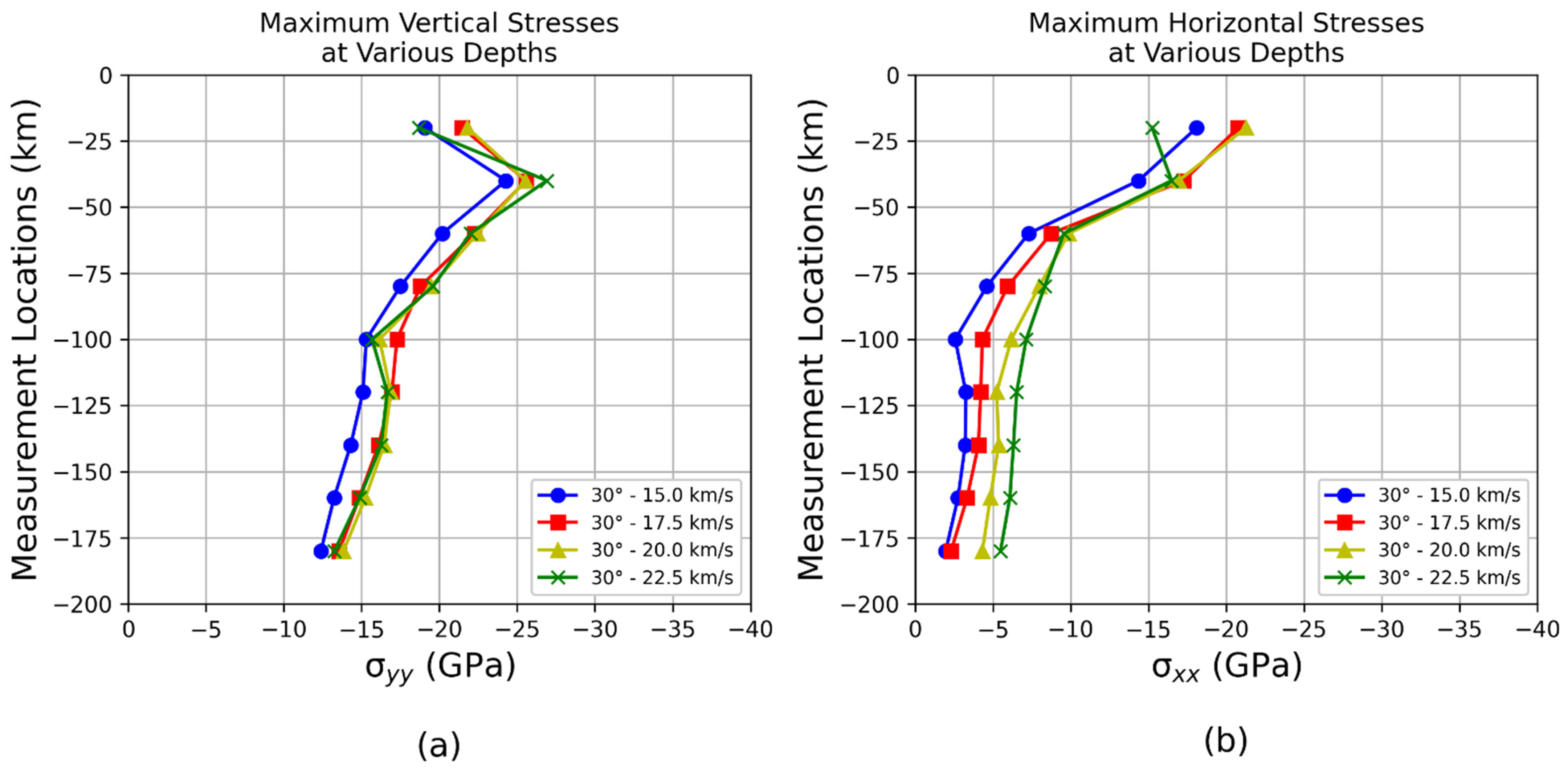
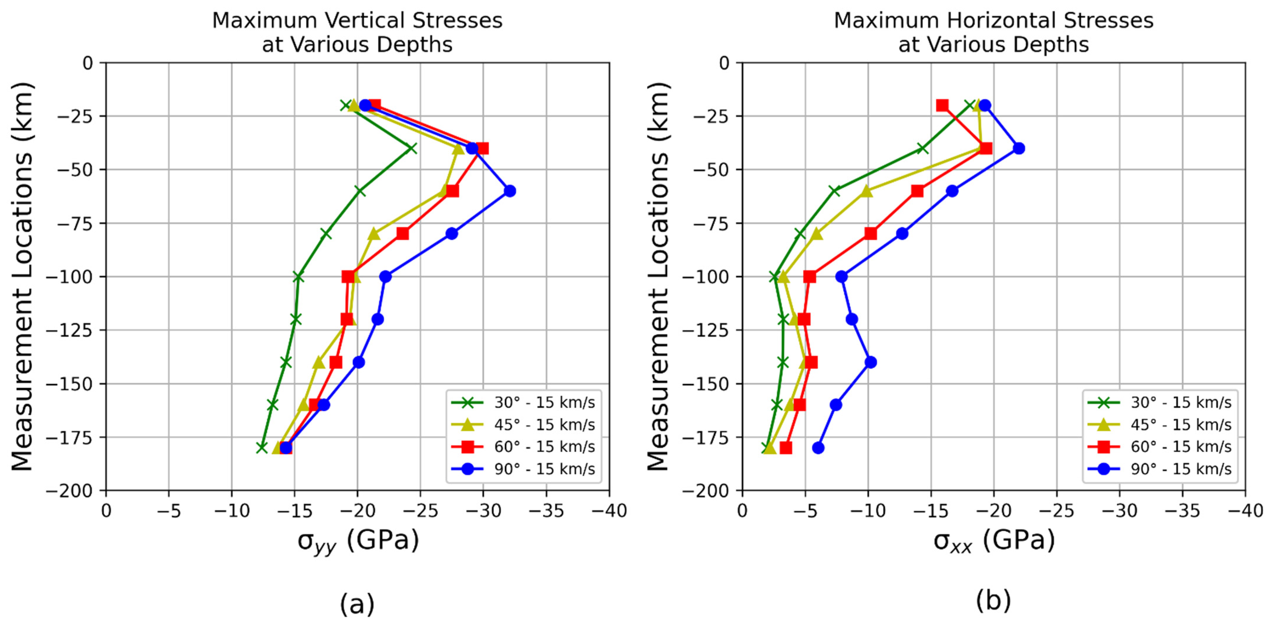
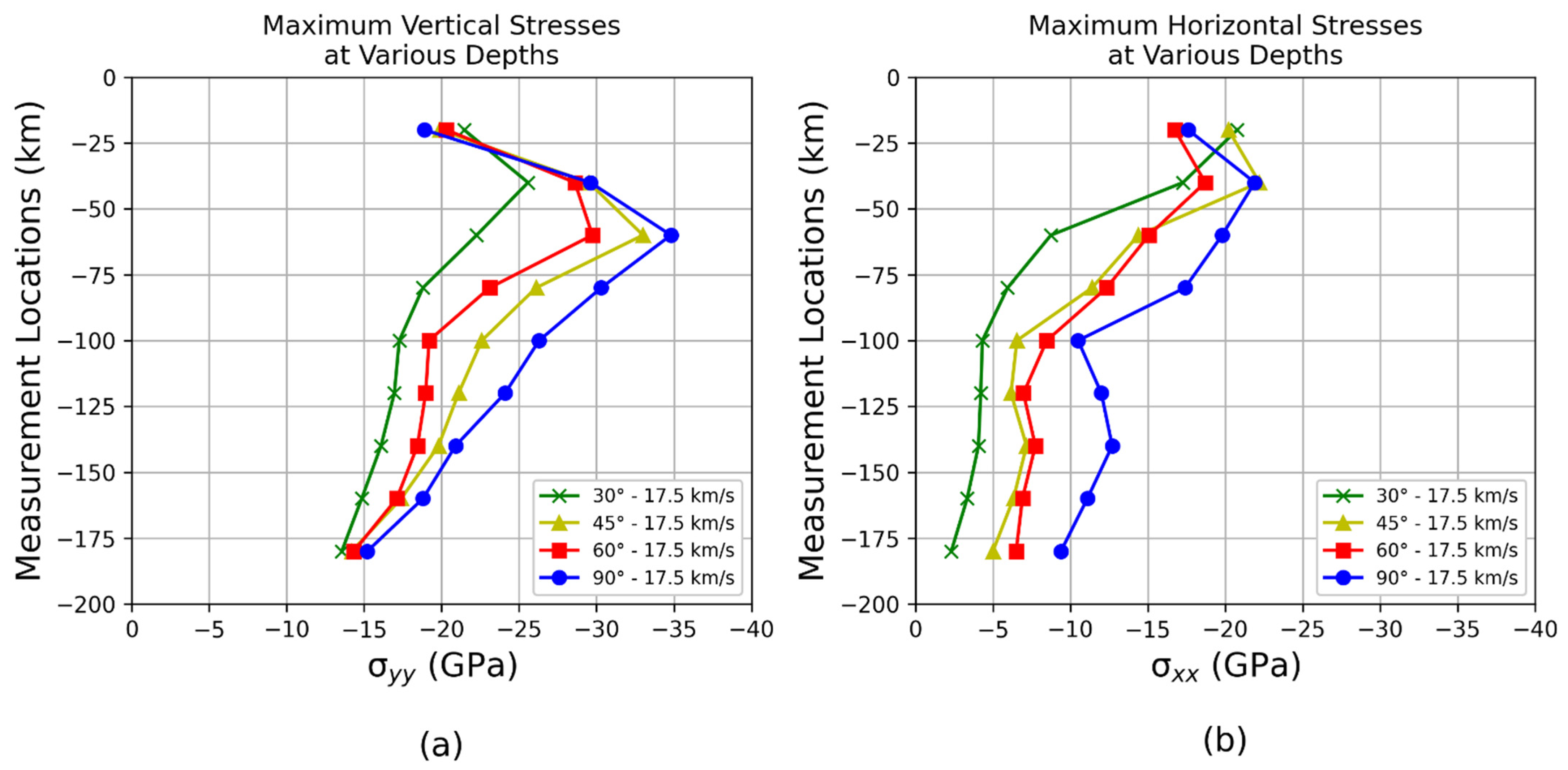
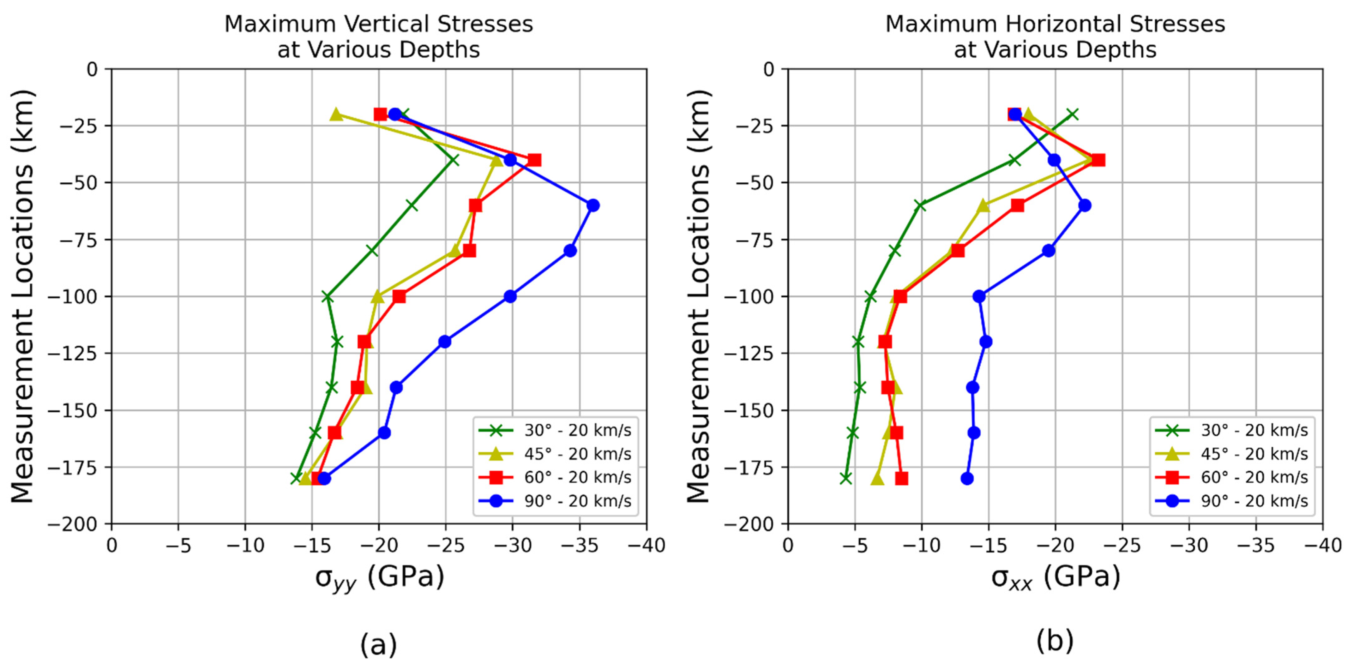
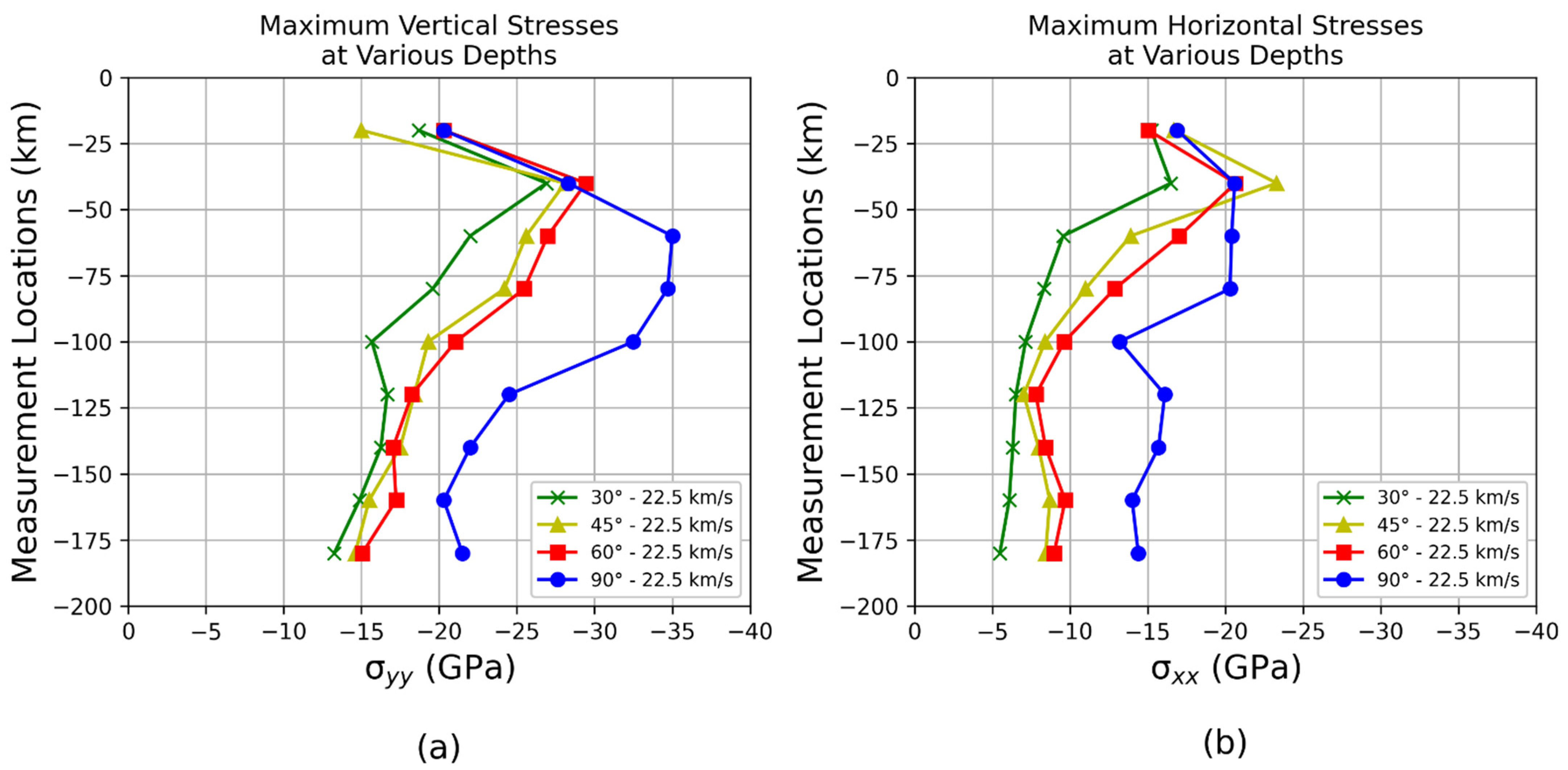
5.4. Horizontal and Vertical Stresses

To further understand the mechanical process of an asteroid impact, stress profiles in both horizontal and vertical directions were recorded at different depths along the centerline of the model container (using the control circles shown in Figure 6). Sequences of stress variation at different depths during the asteroid impact process are shown in Figure 9. Stress measurements show immediate peak variations after impact, which effects last for about 8 s (an observation that is consistent in all control circles, as shown in Figure 6) with dissipating stresses with respect to depth, in addition to the accumulation of stresses with respect to depth.
Figure 10, Figure 11, Figure 12 and Figure 13 compare the maximum stress experienced for the cases of different asteroid impact velocities and similar impact angles. These figures showed that the maximum vertical stresses were always larger than the maximum horizontal stresses. The highest stresses were mostly seen at the depth of 40 km below the ground surface, varying around 30 GPa for vertical direction and around 20 GPa for horizontal direction. The effect of changing impact velocity was noticeable for 90° impacts, while there was hardly any difference in maximum vertical stresses for smaller angular impacts. In the horizontal direction, the variation in velocity showed a higher difference in maximum stress, especially after 60 km depth. For the first 40 km depth, there was no clear effect of velocity to the recorded stresses. On the other hand, Figure 14, Figure 15, Figure 16 and Figure 17 compare the maximum stress experienced for the cases of different impact angles and similar asteroid velocity. In general, maximum stresses decreased as the impact angle decreased. These observations were consistent with the impact process, which further validated the use of the DEM modeling approach.

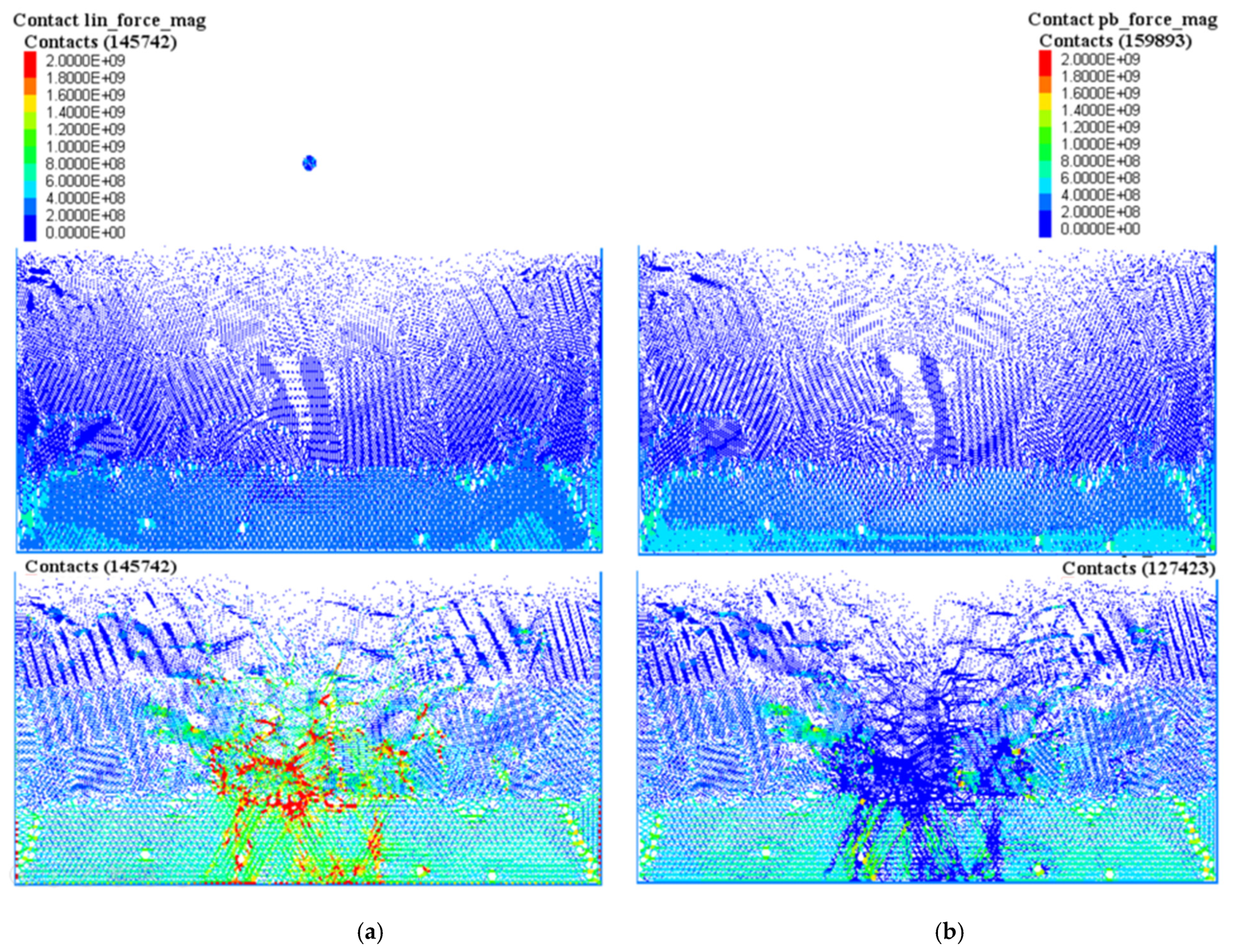
5.5. Contact Force Chains

A final representation of the asteroid impact worth exploring in PFC2D are the maps of contact force chains obtained for both the ‘linear contact model’ and the ‘linear parallel bond contact model’. Figure 18 shows the changes in the force chains before and after the impact, for the case of a 90° impact angle with an asteroid impact velocity of 15 km/s. This sequence showed that particles formed distinct configurations of contact particle forces before and after the impact. A series of contact networks were formed, with higher contact forces developing at the center of the model container after impact; these had a higher order of magnitude in the case of no contact bonding (i.e., linear contact), and a better distribution of the contact forces when contact bonding was present (i.e., linear parallel bond). Also, it was noticed that a series of compression waves moved away from the center line after impact. These observations were also consistent with the expected mechanistic response during the impact process.

6. Conclusions

This study has provided a quantitative and parametric numerical assessment of an asteroid impact on Earth using a DEM model formulated in PFC2D. This was compared with recent structural stratigraphic representation of the Chicxulub crater. Different impact scenarios were generated by varying asteroid velocity and impact angles to match the target crater topography obtained from geological and geophysical investigations. A number of variables were analyzed that helped validate the expected response of the asteroid’s impact, including topography, stratigraphy, stresses, and velocities.
Results showed consistently that the proposed DEM models produced simple craters, but also offered proof that the mechanical model response was consistent with the impact, both near and far field, which had not been proven before. This illustrated that the DEM models can reproduce the phenomenological suction effect of complex craters, observed when materials from deeper strata are pulled from the center of the impact, up to the surface of the crater footprint. This may be an indication that further investigations using DEM may be capable of reproducing complex craters. From the two control variables defined in the experimental design (asteroid’s impact velocity and inclination), it was observed that the uplifting effect was governed by the impact velocity, while the shearing effect was caused by impact angles. Also, the final crater configuration suggested that oblique impacts produce more uplift effects at the crater rims in an upward direction and more excavation in a downward direction.
The use of a quantitative analysis based on MSE values (and comparing the DEM discontinuous vs. continuous media formulations) showed that DEM reproduced the most likely topographic representations of the Chicxulub crater across various combinations of velocity and inclinations.

Author Contributions

Conceptualization, T.N.-M.D., B.H., Z.M.-C. and J.U.F.; methodology, T.N.-M.D., B.H., Z.M.-C. and J.U.F.; software, T.N.-M.D., B.H.; validation, T.N.-M.D., B.H., Z.M.-C. and J.U.F.; formal analysis, T.N.-M.D., B.H., Z.M.-C. and J.U.F.; investigation, T.N.-M.D., B.H., Z.M.-C. and J.U.F.; resources, T.N.-M.D., Z.M.-C. and J.U.F.; data curation, T.N.-M.D., B.H.; writing—original draft preparation, T.N.-M.D., B.H., Z.M.-C.; writing—review and editing, T.N.-M.D., B.H., Z.M.-C. and J.U.F.; visualization, T.N.-M.D., B.H.; supervision, Z.M.-C.; project administration, Z.M.-C.; funding acquisition, T.N.-M.D., Z.M.-C. and J.U.F. All authors have read and agreed to the published version of the manuscript.

Funding

Work presented in this paper was sponsored by the Texas A&M University: Zachry Career Development Professorship II; the Norwegian Geotechnical Institute: Research Development Grant + Fundacion de Ciencias Chicxulub.

Data Availability Statement

The experimental data supporting the findings of this paper are provided along with the article and made available at the Texas Data Repository (https://dataverse.tdl.org/dataverse/SGL-MDPI-Topic-StochasticGeomechancis-ForwardModeling, accessed on 2 May 2023) Additional queries may be directed to the corresponding author.

Conflicts of Interest

The authors declare no conflicts interest.

Appendix A. Final Crater Profile and Crater Evolution

Appendix A.1. Final Crater Profile after 2 Million Calculation Cycles

Figure A1. Final craters, corresponding to different asteroid velocities of 10 km/s (a), 12.5 km/s (b), 15 km/s (c), 17.5 km/s (d), 20 km/s (e), and 22.5 km/s (f), at an impact angle 90°.
Geosciences 13 00139 g0a1aGeosciences 13 00139 g0a1b
Figure A2. Final craters, corresponding to different asteroid velocities of 10 km/s (a), 12.5 km/s (b), 15 km/s (c), 17.5 km/s (d), 20 km/s (e), and 22.5 km/s (f), at an impact angle 60°.
Geosciences 13 00139 g0a2aGeosciences 13 00139 g0a2b
Figure A3. Final craters, corresponding to different asteroid velocities of 10 km/s (a), 12.5 km/s (b), 15 km/s (c), 17.5 km/s (d), 20 km/s (e), and 22.5 km/s (f), at an impact angle of 45°.
Geosciences 13 00139 g0a3aGeosciences 13 00139 g0a3b
Figure A4. Final craters, corresponding to different asteroid velocities of 10 km/s (a), 12.5 km/s (b), 15 km/s (c), 17.5 km/s (d), 20 km/s (e), and 22.5 km/s (f), at an impact angle of 30°.
Geosciences 13 00139 g0a4aGeosciences 13 00139 g0a4b

Appendix A.2. Evolution of the Crater Impact

Figure A5. Velocity field variation right after impact at 90° and asteroid velocity of 15 km/s, at calculation cycles of 5000 (a), 10,000 (b), 15,000 (c), 20,000 (d), 40,000 (e), and 80,000 (f).
Geosciences 13 00139 g0a5
Figure A6. Velocity field variation right after impact at 60° and asteroid velocity of 15 km/s, at calculation cycles of 5000 (a), 10,000 (b), 15,000 (c), 20,000 (d), 40,000 (e), and 80,000 (f).
Geosciences 13 00139 g0a6
Figure A7. Velocity field variation right after impact at 45° and asteroid velocity of 15 km/s, at calculation cycles of 5000 (a), 10,000 (b), 15,000 (c), 20,000 (d), 40,000 (e), and 80,000 (f).
Geosciences 13 00139 g0a7
Figure A8. Velocity field variation right after impact at 30° and asteroid velocity of 15 km/s, at calculation cycles of 5000 (a), 10,000 (b), 15,000 (c), 20,000 (d), 40,000 (e), and 80,000 (f).
Geosciences 13 00139 g0a8
Figure A9. Velocity field variation right after impact at 90° and asteroid velocity of 22.5 km/s, at calculation cycles of 5000 (a), 10,000 (b), 15,000 (c), 20,000 (d), 40,000 (e), and 80,000 (f).
Geosciences 13 00139 g0a9
Figure A10. Velocity field variation right after impact at 60° and asteroid velocity of 22.5 km/s, at calculation cycles of 5000 (a), 10,000 (b), 15,000 (c), 20,000 (d), 40,000 (e), and 80,000 (f).
Geosciences 13 00139 g0a10
Figure A11. Velocity field variation right after impact at 45° and asteroid velocity of 22.5 km/s, at calculation cycles of 5000 (a), 10,000 (b), 15,000 (c), 20,000 (d), 40,000 (e), and 80,000 (f).
Geosciences 13 00139 g0a11
Figure A12. Velocity field variation right after impact at 30° and asteroid velocity of 22.5 km/s, at calculation cycles of 5000 (a), 10,000 (b), 15,000 (c), 20,000 (d), 40,000 (e), and 80,000 (f).
Geosciences 13 00139 g0a12

References

  1. Schulte, P.; Alegret, L.; Arenillas, I.; Arz, J.A.; Barton, P.J.; Bown, P.R.; Bralower, T.J.; Christeson, G.L.; Claeys, P.; Cockell, C.S.; et al. The Chicx-ulub asteroid impact and mass extinction at the Cretaceous-Paleogene boundary. Science 2010, 327, 1214–1218. [Google Scholar] [CrossRef]
  2. Salguero-Hernandez, E.; Urrutia-Fucugauchi, J.; Ramirez-Cruz, L. Fracturing and Deformation in the Chicxulub Crater—Complex Trace Analysis of Instataneous Seismic Attributes. Rev. Mex. Cienc. Geol. 2011, 27, 175–184. [Google Scholar]
  3. Urrutia-Fucugauchi, J.; Camargo–Zanoguera, A.; Pérez–Cruz, L.; Pérez–Cruz, G. The Chicxulub Multi-Ring Impact Cra-ter, Yucatan Carbonate Platform, Gulf of Mexico. Geofis. Int. 2011, 50, 99–127. [Google Scholar]
  4. Gulick, S.P.S.; Christeson, G.L.; Barton, P.J.; Grieve, R.A.F.; Morgan, J.V.; Urrutia-Fucugauchi, J. Geophysical characteri-zation of the Chicxulub impact crater. Rev. Geophys. 2013, 51, 31–52. [Google Scholar] [CrossRef]
  5. Urrutia-Fucugauchi, J.; Perez-Cruz, L. Chicxulub Asteroid Impact: An Extreme Event at the Cretaceous/Paleogene Boundary. In Extreme Events: Observations, Modeling, and Economics; Geophysical Monograph Series 214; Chavez, M., Ghil, M., Urrutia-Fucugauchi, J., Eds.; Wiley-Blackwell: Hoboken, NJ, USA, 2016. [Google Scholar]
  6. Holsapple, K.A.; Schmidt, R.M. On the scaling of crater dimensions: 1. Explosive processes. J. Geophys. Res. Atmos. 1980, 85, 7247–7256. [Google Scholar] [CrossRef]
  7. Holsapple, K.A.; Schmidt, R.M. On the scaling of crater dimensions: 2. Impact processes. J. Geophys. Res. Atmos. 1982, 87, 1849–1870. [Google Scholar] [CrossRef]
  8. Austin, M.G.; Thomsen, J.M.; Ruhl, S.F.; Orphal, D.L.; Borden, W.F.; Larson, S.A.; Schultz, P.H. Z-Model Analysis of Impact Cratering: An Overview. Multi-ring Basins: Formation and Evolution. In Proceedings of the Lunar and Planetary Science Conference, Houston, TX, USA, 10–12 November 1980. [Google Scholar]
  9. Takata, T.; Ahren, T.J. Numerical Simulation of Impact Cratering at Chicxulub and the Possible Causes of KT Catastrophe; Lunar and Planetary Institute: Houston, TX, USA, 1994; p. 125. [Google Scholar]
  10. Ivanov, B.A.; Badukov, D.D.; Yakovlev, O.L.; Gerasimov, M.V.; Dikov, Y.P.; Pope, K.O.; Ocampo, A.C. Degassing of Sed-imentary Rocks Due to Chicxulub Impact: Hydrocode and Physical Simulations. Cretac.-Tert. Event Other Catastr. Earth Hist. 1996, 307, 125–139. [Google Scholar]
  11. Morgan, J.V.; Gulick, S.P.S.; Bralower, T.; Chenot, E.; Christeson, G.; Claeys, P.; Cockell, C.; Collins, G.S.; Coolen, M.J.L.; Ferrière, L.; et al. The formation of peak rings in large impact craters. Science 2016, 354, 878–882. [Google Scholar] [CrossRef] [PubMed]
  12. Robertson, D.K.; Mathias, D.L. Hydrocode simulations of asteroid airbursts and constraints for Tunguska. Icarus 2018, 327, 36–47. [Google Scholar] [CrossRef]
  13. Pierazzo, E.; Melosh, H.J. Hydrocode modeling of Chicxulub as an oblique impact event. Earth Planet. Sci. Lett. 1999, 165, 163–176. [Google Scholar] [CrossRef]
  14. Collins, G.S.; Melosh, H.J.; Marcus, R.A. Earth Impact Effects Program: A Web-based computer program for calculating the regional environmental consequences of a meteoroid impact on Earth. Meteorit. Planet. Sci. 2005, 40, 817–840. [Google Scholar] [CrossRef]
  15. Ivanov, B.A. Large Impact Crater Modeling: Chicxulub. In Proceedings of the Third International Conference on Large Meteorite Impacts, Nordlingen, Germany, 5–7 August 2003. [Google Scholar]
  16. Collins, G.S.; Morgan, J.; Barton, P.; Christeson, G.L.; Gulick, S.; Urrutia, J.; Warner, M.; Wünnemann, K. Dynamic modeling suggests terrace zone asymmetry in the Chicxulub crater is caused by target heterogeneity. Earth Planet. Sci. Lett. 2008, 270, 221–230. [Google Scholar] [CrossRef]
  17. Collins, G.S.; Wünnemann, K.; Artemieva, N.; Pierazzo, E. Numerical Modelling of Impact Processes. In Impact Cratering; Osinski, G.R., Pierazzo, E., Eds.; Blackwell: Oxford, UK, 2012; pp. 254–270. [Google Scholar] [CrossRef]
  18. Collins, G.S.; Patel, N.; Davison, T.M.; Rae, A.S.P.; Morgan, J.V.; Gulick, S.P.S.; Christeson, G.L.; Chenot, E.; Claeys, P.; Cockell, C.S.; et al. A steeply-inclined trajectory for the Chicxulub impact. Nat. Commun. 2020, 11, 1480. [Google Scholar] [CrossRef] [PubMed]
  19. Collins, G.S.; Patel, N.; Rae, A.S.P.; Davison, T.M.; Morgan, J.V.; Gulick, S.; Expedition 364 Scientists. Numerical Simulations of Chicxulub Crater Formation by Oblique Impact. In Proceedings of the Lunar and Planetary Science XLVIII Conference, Houston, TX, USA, 20–24 March 2017. [Google Scholar]
  20. Artemieva, N.; Morgan, J.; Expedition 364 Science Party. Quantifying the Release of Climate-Active Gases by Large Meteorite Impacts with a Case Study of Chicxulub. Geophys. Res. Lett. 2017, 44, 10180–10188. [Google Scholar] [CrossRef]
  21. Amsden, A.A.; Ruppel, H.M. SALE-3D: A Simplified SALE Computer Program for Calculating Three-Dimensional Fluid Flow; Los Alamos National Lab.: Los Alamos, NM, USA, 1981. [Google Scholar]
  22. Gisler, G.; Weaver, R.P.; Mader, C.; Gittings, M. Two- and Three-Dimensional Simulations of Asteroid Ocean Impacts. Sci. Tsunami Harzard 2003, 21, 119–134. [Google Scholar] [CrossRef]
  23. Elbeshausen, D.; Wünnemann, K.; Collins, G.S. Scaling of oblique impacts in frictional targets: Implications for crater size and formation mechanisms. Icarus 2009, 204, 716–731. [Google Scholar] [CrossRef]
  24. McCall, N.; Gulick, S.P.; Hall, B.; Rae, A.S.; Poelchau, M.H.; Riller, U.; Lofi, J.; Morgan, J.V. Orientations of planar cataclasite zones in the Chicxulub peak ring as a ground truth for peak ring formation models. Earth Planet. Sci. Lett. 2021, 576, 117236. [Google Scholar] [CrossRef]
  25. Kring, D.A.; Tikoo, S.M.; Schmieder, M.; Riller, U.; Rebolledo-Vieyra, M.; Simpson, S.L.; Osinski, G.R.; Gattacceca, J.; Wittmann, A.; Verhagen, C.M.; et al. Probing the hydrothermal system of the Chicxulub impact crater. Sci. Adv. 2020, 6, eaaz3053. [Google Scholar] [CrossRef] [PubMed]
  26. Cundall, P.A.; Strack, O.D.L. A discrete numerical model for granular assemblies. Géotechnique 1979, 29, 47–65. [Google Scholar] [CrossRef]
  27. Zhu, H.P.; Zhou, Z.Y.; Yang, R.Y.; Yu, A.B. Discrete particle simulation of particulate systems: A review of major applications and findings. Chem. Eng. Sci. 2008, 63, 5728–5770. [Google Scholar] [CrossRef]
  28. Potyondy, D.O. The bonded-particle model as a tool for rock mechanics research and application: Current trends and future directions. Geosyst. Eng. 2015, 18, 1–28. [Google Scholar] [CrossRef]
  29. Yanbei, Z. Probabilistic Calibration of a Discrete Particle Model. Master’s Thesis, Texas A&M University, College Station, TX, USA, 2010. [Google Scholar]
  30. Noble, P.A. Uncertainty Quantification of the Homogeneity of Granular Materials through Discrete Element Modeling and X-rays Computed Tomography. Master’s Thesis, Texas A&M University, College Station, TX, USA, 2012. [Google Scholar]
  31. Duong, T.N.M.; Hernawan, B.; Medina-Cetina, Z. Experimental and Numerical Assessment of Sample Heterogeneity and Failure Mechanism of Speciments Formed with Granular Material. Minerals 2023. submitted. [Google Scholar]
  32. Ledgerwood, L.W. PFC Modeling of Rock Cutting under High Pressure Conditions. In Proceedings of the 1st Canada—U.S. Rock Mechanics Symposium, Vancouver, BC, Canada, 27–31 May 2007. [Google Scholar]
  33. Giese, S. Numerical simulation of vibroflotation compaction—Application of dynamic boundary conditions. In Numerical Modeling in Micromechanics via Particle Methods; Routledge: New York, NY, USA, 2003; pp. 117–124. [Google Scholar] [CrossRef]
  34. Hardy, S. Discrete Element Modelling of Pit Crater Formation on Mars. Geosciences 2021, 11, 268. [Google Scholar] [CrossRef]
  35. Smart, K.J.; Wyrick, D.Y.; Ferrill, D.A. Discrete element modeling of Martian pit crater formation in response to extensional fracturing and dilational normal faulting. J. Geophys. Res. Planets 2011, 116, 383–392. [Google Scholar] [CrossRef]
  36. Caldwell, W.K.; Euser, B.; Plesko, C.S.; Larmat, C.; Lei, Z.; Knight, E.E.; Rougier, E.; Hunter, A. Benchmarking Numerical Methods for Impact and Cratering Applications. Appl. Sci. 2021, 11, 2504. [Google Scholar] [CrossRef]
  37. Çelik, O.; Ballouz, R.-L.; Scheeres, D.J.; Kawakatsu, Y. A numerical simulation approach to the crater-scaling relationships in low-speed impacts under microgravity. Icarus 2022, 377, 114882. [Google Scholar] [CrossRef]
  38. Zhang, Y.; Jutzi, M.; Michel, P.; Raducan, S.; Arakawa, M. Effect of material strength and heterogeneity on small asteroid cratering events. In Proceedings of the Europlanet Science Congress 2021, online, 13–24 September 2021. [Google Scholar] [CrossRef]
  39. Medina-Cetina, Z. Probabilistic Calibration of a Soil Model. Ph.D. Thesis, Johns Hopkins University, Baltimore, MD, USA, 2007. [Google Scholar]
  40. Medina-Cetina, Z.; Nadim, F. Stochastic design of an early warning system. Georisk: Assess. Manag. Risk Eng. Syst. Geohazards 2008, 2, 223–236. [Google Scholar] [CrossRef]
  41. Medina-Cetina, Z.; Arson, C. Probabilistic calibration of a damage rock mechanics model. Géotech. Lett. 2014, 4, 17–21. [Google Scholar] [CrossRef]
  42. Gulick, S.; Morgan, J.; Mellet, C.L.; Expedition 364 Scientists. Expedition 364 Preliminary Report: Chicxulub: Drilling the K-Pg Impact Crater; International Ocean Discovery Program: College Station, TX, USA, 2017. [Google Scholar] [CrossRef]
  43. Alvarez, L.W.; Alvarez, W.; Asaro, F.; Michel, H.V. Extraterrestrial Cause for the Cretaceous-Tertiary Extinction. Science 1980, 208, 1095–1108. [Google Scholar] [CrossRef] [PubMed]
  44. Hildebrand, A.R.; Pilkington, M.; Ortiz-Aleman, C.; Chavez, R.E.; Urrutia-Fucugauchi, J.; Connors, M.; Graniel-Castro, E.; Camara-Zi, A.; Halpenny, J.F.; Niehaus, D. Mapping Chicxulub crater structure with gravity and seismic reflection data. In Meteorites: Flux with Time and Impact Effects. Geological Society; Graddy, M.M., Hutchinson, R., McCall, G.J.H., Rotherby, D.A., Eds.; Special Publications: London, UK, 1998; Volume 140, pp. 155–176. [Google Scholar] [CrossRef]
  45. Navarro, K.F.; Urrutia-Fucugauchi, J.; Villagran-Muniz, M.; Sánchez-Aké, C.; Pi-Puig, T.; Pérez-Cruz, L.; Navarro-González, R. Emission spectra of a simulated Chicxulub impact-vapor plume at the Cretaceous–Paleogene boundary. Icarus 2020, 346, 113813. [Google Scholar] [CrossRef]
  46. Potyondy, D. Material-Modeling Support in PFC. Technical Memorandum ICG7766-L; Itasca Consulting Group: Minneapolis, MN, USA, 2015. [Google Scholar]
  47. Itasca. PFC3D 7.0 Manual. Particles Flow Code in three Dimensions-PFC3D. 2019s. Available online: https://docs.itascacg.com/pfc700/contents.html (accessed on 2 May 2023).
  48. Trinquier, A.; Birck, J.-L.; Allègre, C.J. The nature of the KT impactor. A 54Cr reappraisal. Earth Planet. Sci. Lett. 2006, 241, 780–788. [Google Scholar] [CrossRef]
  49. Goderis, S.; Sato, H.; Ferrière, L.; Schmitz, B.; Burney, D.; Kaskes, P.; Vellekoop, J.; Wittmann, A.; Schulz, T.; Chernonozhkin, S.M.; et al. Globally distributed iridium layer preserved within the Chicxulub impact structure. Sci. Adv. 2021, 7, eabe3647. [Google Scholar] [CrossRef] [PubMed]
  50. Gelinas, A.; Kring, D.A.; Zurcher, L.; Urrutia-Fucugauchi, J.; Morton, O.; Walker, R.J. Osmium isotope constraints on the proportion of bolide component in Chicxulub impact melt rocks. Meteorit. Planet. Sci. 2004, 39, 1003–1008. [Google Scholar] [CrossRef]
  51. Davison, T.M.; Collins, G.S. Complex Crater Formation by Oblique Impacts on the Earth and Moon. Geophys. Res. Lett. 2022, 49, e2022GL101117. [Google Scholar] [CrossRef]
  52. Kenkmann, T.; Poelchau, M.H.; Wulf, G. Structural geology of impact craters. J. Struct. Geol. 2014, 62, 156–182. [Google Scholar] [CrossRef]
Figure 1. Chicxulub crater with the cross-section of interest ‘Chicx-A/A1′, and the corresponding drilling locations. Reconstructed from Salguero-Hernandez et al. [2].
Geosciences 13 00139 g001
Figure 2. Schematic graph of the model experimental design with varying impact angle and velocity (highlighted in red font).
Geosciences 13 00139 g002
Figure 3. Aerial map of the Yucatán Peninsula. Peak ring center, crater center, and mantle uplift center are marked, along with the cross-section of interest, Chicx-A/A1. Approximate surface topography, produced using 3D iSALE hydrocode for an impact direction from northeast to southwest [18,19], is also shown above for an asteroid impact of 60° at 12 km/s. Area bounded by the red line indicates the region with uplift, while the blue line indicates the region of depression. This image was reconstructed with data from Salguero-Hernandez et al. [2] and by Collins et al. [19].
Geosciences 13 00139 g003
Figure 4. Asteroid impact model configuration.
Geosciences 13 00139 g004
Figure 5. Verification of the infinite boundary condition. Red particle is a rolling ball exerting a force in resting particles 1–5 who serve as control points to assess the influence of the boundary condition.
Geosciences 13 00139 g005
Figure 6. Locations of the 200 m control circles along the centerline and 20 m control circles along the wall boundaries. Colors or the circles only represent their independent locations.
Geosciences 13 00139 g006
Figure 7. Crater topographies for 90° (a), 60° (b), 45° (c), and 30° (d) impact angles at various speeds. Reconstructed topography from Collins et al. [18] was retrieved from the plane of the intersection of interest.
Geosciences 13 00139 g007aGeosciences 13 00139 g007b
Figure 8. Mean squared error (MSE) surface of different combinations of velocity and impact angle. The red plot markers represent the profile simulated using PFC2D presented in this study, while the black plot markers represent the reconstructed profile from Collins et al. [19].
Geosciences 13 00139 g008
Figure 9. Vertical stress (a) and horizontal stress (b) histories for asteroid impacts at a velocity of 15 km/s with an impact angle of 90°.
Geosciences 13 00139 g009
Figure 10. Maximum vertical stress (a) and maximum horizontal stress (b) for asteroid impacts at 90° impact angle and with various velocities.
Geosciences 13 00139 g010
Figure 11. Maximum vertical stress (a) and maximum horizontal stress (b) for asteroid impacts at 60° impact angle and with various velocities.
Geosciences 13 00139 g011
Figure 12. Maximum vertical stress (a) and maximum horizontal stress (b) for asteroid impacts at 45° impact angle and with various velocities.
Geosciences 13 00139 g012
Figure 13. Maximum vertical stress (a) and maximum horizontal stress (b) for asteroid impacts at 30° impact angle and with various velocities.
Geosciences 13 00139 g013
Figure 14. Maximum vertical stress (a) and maximum horizontal stress (b) for asteroid impacts at 15 km/s and with different impact angles.
Geosciences 13 00139 g014
Figure 15. Maximum vertical stress (a) and maximum horizontal stress (b) for asteroid impacts at 17.5 km/s and with different impact angles.
Geosciences 13 00139 g015
Figure 16. Maximum vertical stress (a) and maximum horizontal stress (b) for asteroid impacts at 20 km/s and with different impact angles.
Geosciences 13 00139 g016
Figure 17. Maximum vertical stress (a) and maximum horizontal stress (b) for asteroid impacts at 22.5 km/s and with different impact angles.
Geosciences 13 00139 g017
Figure 18. Maps of linear contact force chains (a) and linear parallel bond contact force chain (b) before (top row) and after (bottom row) asteroid impact at a velocity of 15 km/s at an impact angle of 90°.
Geosciences 13 00139 g018
Table 1. Layer parameters used in the model.
LayerMaterialLayer Depth (m)Particle Diameter (m)
1Sedimentary Limestone105
2305
3Rock Basement905
418010
518010
618010
736020
836020
961040
Table 2. Contact bond model properties used in PFC2D.
NameContact TypeParticle
Normal Stiffness
Particle
Shear Stiffness
Friction CoefficientBond Normal StiffnessBond Shear StiffnessBond TensionBond Cohesion
PaPa-PaPaNN
AsteroidLinear parallel bond4.0 × 1091.6 × 1090.34.0 × 1091.6 × 1094.0 × 1064.0 × 106
Sedimentary limestoneLinear parallel bond4.0 × 1091.6 × 1090.34.0 × 1091.6 × 1094.0 × 1064.0 × 106
Rock basementLinear parallel bond40.0 × 10916.0 × 1090.340.0 × 10916.0 × 10940.0 × 10640.0 × 106
WallsLinear contact5 × 10105 × 10100----
Disclaimer/Publisher’s Note: The statements, opinions and data contained in all publications are solely those of the individual author(s) and contributor(s) and not of MDPI and/or the editor(s). MDPI and/or the editor(s) disclaim responsibility for any injury to people or property resulting from any ideas, methods, instructions or products referred to in the content.

