Numerical Simulation of Rockfall Protection Embankments in Natural Soil

Abstract

Rockfall events represent a significant hazard in mountainous regions, putting human safety and critical infrastructure at risk. Various mitigation devices are available, among which, Rockfall protection embankments (RPEs) located in natural soil are passive defense work suitable for high-energy and high-frequency events. Currently, limited research has been conducted in this area, with the Austrian standard ONR 24810 providing the sole codified design method. A parametrical analysis involving both the RPE geometry and the impact features was developed by Abaqus/Explicit FEM code, with 2270 cases overall. The research aims to identify conditions under which RPEs effectively stop falling blocks, focusing on two failure mechanisms: the block pass over the RPE after impacting the upstream side bank and the RPE structural collapse. Additionally, the interaction between RPEs and their foundations during the impact is explored. The results provide valuable insights into the dynamic behavior of these structures. In terms of design considerations, this study offers analytical equations to quantify crater depth and foundation stress induced by the impact. Furthermore, design charts are developed to assess the block passing over verification and the structural collapse verification.

1. Introduction

Rockfall phenomena are a significant hazard that affects mountain areas [1,2,3]; due to the effects of climate change, they are increasing in frequency [4]. Rockfall puts at risk the safety of human life and the use of important infrastructures such as roads, railways [5,6,7,8,9], connecting municipalities, and touristic areas.

To mitigate this hazard, there are many methods available [2] (i.e., rockfall barriers, rockfall-shed, embankments, etc.) that differ in terms of their potential energy capacity, the dimensions required for their installation, their costs, and, last but not least, their installation times. The rockfall protection embankment (RPE) typologies are many. 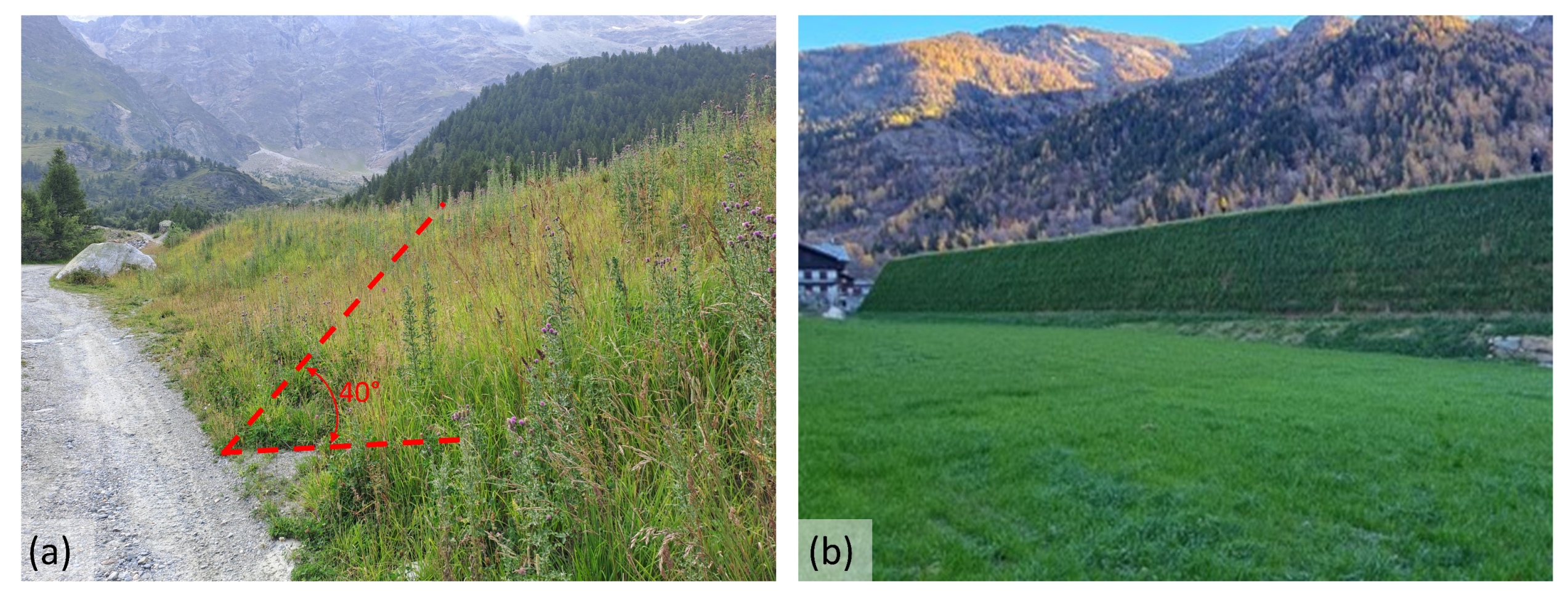Some technological classifications according to the materials used were reported in [10,11,12]. However, the simplest difference can be made between embankments made only of compacted soil and those made of reinforced soil. The first reaches relatively low side slopes of the order of 30°–40°; instead, the seconds are typically made with reinforced high-density polyethylene (HDPE) geogrids or double-twisted wire mesh in order to achieve side slopes of up to 70°. In Figure 1, two examples are reported.

The characteristic of RPEs is that being built on site by assembling mainly granular material, they are the only ones capable of meeting the energy demand from a few hundred kilojoules to tens of megajoules by increasing their size, as well as being suitable in situations of frequent impacts requiring little maintenance [11,13,14]. Usually, RPEs are the preferred technology when the design impact energy is higher than 5000 kJ [9,11] and where the slope and available space are adequate to prevent the global instability [9,11,14,15].

Due to the importance of these structures, the designers and public administrations need suitable design tools and procedures [1,7,16].

Nowadays, the prevailing choice of construction falls on reinforced RPEs [9,14] due to the advantages of the reduced soil occupation and used material; nevertheless, the non-reinforced typology is of interest to designers and local authorities in special situations, for example, urgent interventions or the local and small-scale protection of buildings in high-altitude mountain environments. Low-cost protection applications such as those typically required in the field of mining have already been reported in the literature [17].

Numerous applications were widely used in the past, sometimes without a specific design calculation. Until now, limited studies as well as codified design approaches have been developed to achieve this purpose.

The present research provides insights into the behavior of this intervention type when impacted. A review of the current state of the art in the field (Section Literature Analysis) identifies the two primary failure mechanisms of natural-soil RPEs in dynamic conditions. Since experimental approaches are limited due to their costly and challenging nature, the problem is studied by employing a FEM dynamic numerical model (ABAQUS/Explicit). This research aims to develop simplified design tools for the dynamic design of RPEs without the need for complex numerical modeling.

The soil mechanical parameters are calibrated by plate load test (PLT) data (Section 2.1). To simplify the calibration, a preliminary sensitivity analysis is conducted to determine which parameters have the most significant impact on the results of the RPE impact problem. Only the three most influential parameters were varied in the calibration of the PLTs (Section 2.1.1); furthermore, a validation of the calibrated soil mechanical parameters was carried out by simulating some triaxial test (Section 2.1.2). Subsequently, an extensive parametric analysis was implemented to evaluate the influence of the RPE geometry, impact kinetics, and geometric characteristics with respect to the two RPE failure mechanisms (Section 2.2).

A definition of structural collapse is provided based on the continuous numerical approach in use (Section 3.1). The two mechanisms of failure, namely the block overcoming the RPE and RPE structural collapse, are individuated for the simulated case and are used to create design charts useful to assess them (Section 3.2 and Section 3.3). Moreover, analytical equations are developed to assess the upstream crater and the stresses on the foundation stemming from the impact (Section 3.4).

Literature Analysis

Regarding the full-scale tests, most of these were developed on reinforced RPEs [13,14,18,19,20,21,22,23].

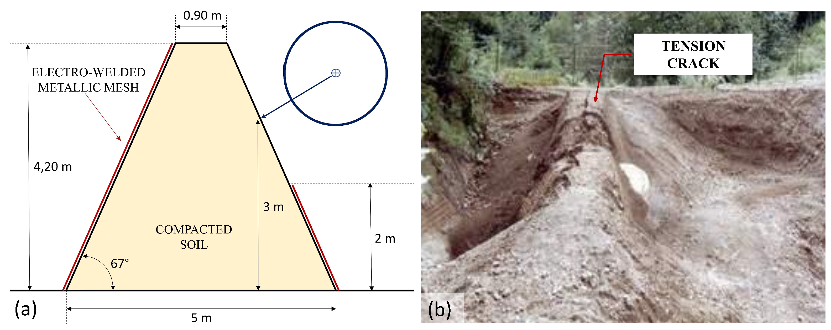
One full-scale test was conducted by Peila et al. (2007) on an RPE in compacted soil with a trapezoidal section and sides of about 67°: this face inclination was obtained using electro-welded metal mesh as a formwork and subsequently removed in the impacted area as shown in Figure 2. The tested embankment stopped the block but the impact induced the collapse of the structure.

To overcome the costs and technical complexity of full-scale tests [24], some small-scale tests have been developed. Hofmann and Mölk (2012) [15] carried out a total of 116 tests in a scale of 1:33, analyzing different embankment typologies: compacted sand-soil, reinforced sand-soil with geogrids, with a rip-rap face and with a damping layer. The impacts block was a 2 kg metal sphere driven in motion with a PVC guide. These test data [11] are at the basis of the codified design methodology inserted in the Austrian standard ONR 24810 (2021) [25]. In the standard, the impact by the rockfall is considered an exceptional design situation, and the RPE design only addresses the ultimate limit state. The design situation is determined by the 99th percentile of the kinetic energy distribution ($E_{k,99\%}$) obtained from the analysis of the trajectories. According to Lambert and Bourrier [9], the design methodology falls under the classification of “analytical energy approaches” and requires the definition of the impact disturbed zone (IDZ)—or rather the volume of the RPE exposed to severe loading resulting in large displacements, strains, and changes in the mechanical characteristics [11]. 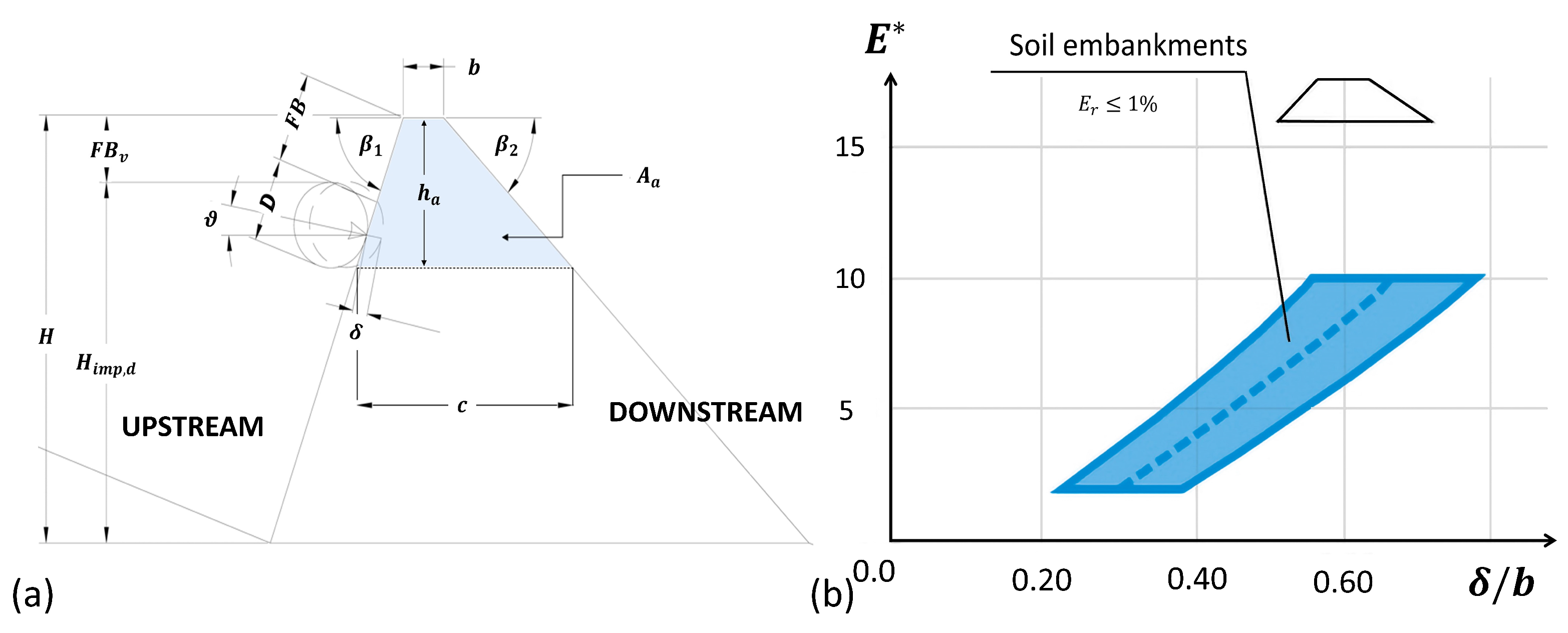Figure 3a shows how the IDZ section was defined by the reduced-scale tests [15,25]. This definition is in agreement with the one proposed by Tissières [20] and similar to that of Subrin et al. [26]. The third dimension of the IDZ is the longitudinal distance of RPE affected by the impact: in the case of loose embankments, the authors identified a value between 5 and 6 times the diameter of the block D [15]. According to the standard [25], it is necessary to compute the so-called “dimensionless impact energy” $E^{*}$ as defined in Equation (1) [25], in which $\gamma$ is the RPE soil density, $A_a$ is defined according to Figure 3a, D is the diameter of the equivalent design block, and $h_a$ is the activated height. Subsequently, the graph in Figure 3b allows one to obtain the relationship between the depth of the crater $\delta$ and the RPE width crest b.

$$E^{*}=\frac{E_{k,99\%}}{\gamma ·A_a·D·h_a}$$

(1)

Finally, the proposed design checks are pseudo-static by applying an equivalent static force $F_k$ (Equation (2)) at the impact point and distributed over a length approximately to $5÷6·D$, which must be amplified by a safety factor ${\gamma }_{E,kin}$ to obtain the design value $F_d$ [25]. Here, m and v are, respectively, the mass and velocity of the design block, while $\Delta t$ is, according to pulse theory, the impact duration estimable between 0.05 s and 0.15 s for non-reinforced RPEs [15].

$$F_k=\frac{v^{2}m}{\delta }=\frac{2vm}{\Delta t}$$

(2)

As can be seen in Figure 3b, the design graph is valid for block rotational energies that are less than 1%; nevertheless, there are no data supporting these limits.

Hofmann and Mölk (2012) [15] noted that the hazard that the block overcomes by rolling or bouncing the structure is the most critical one in natural soil RPEs and, for this reason, they indicated the minimum free-border $FB$ (Figure 3a) equal to two times the diameter of the sphere for embankments with face inclinations lower than 50°.

Kister (2015) [27] performed 34 experiments under near-2D conditions with a scale factor $\lambda =9$. Most of the tests have rocky side banks (masonry stones) and only five tests concerned the RPE without cover [27]. The experimental combinations concern three types of impactors with different impact angles, three slope values for the upstream and downstream banks, two types of soil, and different RPE crests values [11,27]. 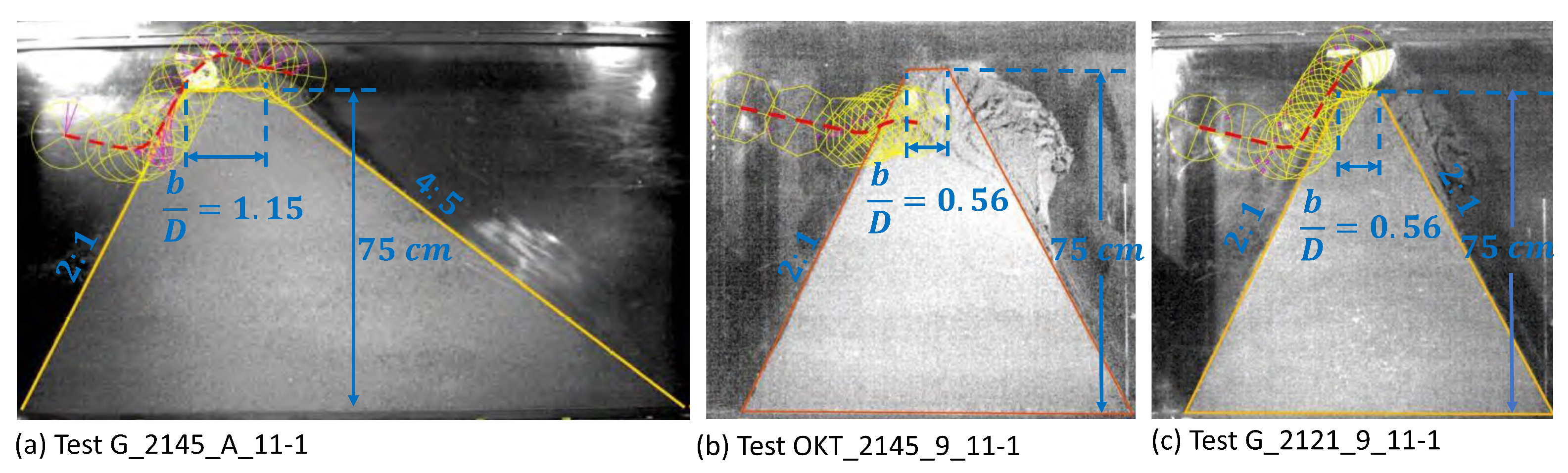Figure 4 shows the images obtained with a high-speed camera during the tests in which collapse was reached. In this research, the collapse is defined when the structure does not contain the block due to the structural collapse or the overcoming of the block beyond the structure. Three collapse mechanisms were generated: the embankment resisted upon impact from a structural point of view but the block climbed along the bank (Figure 4a); the impact induced the collapse of the affected area, even if the trajectory of the block did not go beyond the embankment (Figure 4b); finally, the situation in which the two previous cases occur simultaneously (Figure 4c). Tests on rockery RPEs brought to structural collapse by successive impacts showed the tension crack observed by Peila et al. (2007) [14].

Numerous numerical simulations concerning reinforced RPEs are available in the literature referred to herein [14,28,29,30,31,32]; however, those that only refer to natural soil RPEs are relatively limited [24,29].

Plassiard and Donzé [24,33,34] developed a DEM parametrical analysis on natural soil RPEs, to determine the efficiency range for a given set of geometrical and mechanical properties. The constitutive law of the soil is calibrated based on three energy levels [24,33]: the quasi-static behavior was set up using triaxial test of the soil reported in [34], the Montani [35] drop test at at energies between 50 to 100 kJ and the hight energy level drop test in the range from 1000 to 10,000 kJ of Pichler et. al., 2005 [36]. The geometry of the embankment was established with a height of the structure equal to 5 m, a crest of 2 m, bank inclinations equal to 60° and impact height equal to 2/3 of the total. The impact was carried out with an energy of about 2000 kJ: block diameter D = 1.97 m (mass of 10,600 kg) animated with a purely horizontal translational velocity of v = 19.40 m/s. The authors observed a tendency of the block to cross the embankment as the slope of the upstream slope decreased, associated with the decrease in damage to the work [24]. The simulations have shown how energy alone cannot be considered as the only design parameter, as different combinations of diameter and velocity provide the same force to the structure but with different post-impact trajectories [33] compromising the overcoming verification; furthermore, the pair D-v and the angle of the velocity vector of the block, parameters which are neglected in usual design practice, are not negligible for this verification [33].

2. Methodology: Numerical Model of Block Impact

The numerical analyses of natural soil RPEs impacted by a block were carried out with the FEM code Abaqus/Explicit (Abaqus license: 24, Site ID: 200000000050742).

The soil mechanical parameters are calibrated based on PLT data and the chosen constitutive law. The constitutive law involves a total of six parameters (described in Section 2.1) and, to simplify the calibration process, a preliminary sensitivity analysis regarding an impacted RPE was set up. This analysis only varied the soil mechanical parameters and focused on understanding which among them exert the most significant influence on the outcomes. Subsequently, the most influential parameters are calibrated by PLT data.

The calibrated parameters are utilized to validate the soil behavior in standard triaxial tests (Section 2.1.2).

Subsequently, the calibrated parameters will be applied in an extensive parametric analysis of the impacted RPEs (Section 2.2) involving both the RPE geometry and the features of the impacts.

2.1. Calibration of the Soil Mechanical Parameters

A preliminary sensitivity analysis regarding the RPE impacted by a block problem is carried out and presented in the present section. The fixed input parameters for the RPE impact configuration used in the sensitivity analysis are detailed in

Table 1. Parameters of the sensitivity analysis on parameters of the soil constitutive model.

RPE Geometry			Impactor Features
Height	H	5 m	Sphere radius	R	0.5 m
Sides slope	$\beta$	${40}^{\circ }$	Speed	v	20 m/s
Crest thickness	b	2 m	Angular velocity	$\omega$	5 rad/s
Impact height	$H_{imp}$	$0.5·H$	Speed vector angle	$\alpha$	${90}^{\circ }$

, which refer to the section in the cross-section scheme in Figure 5. The compacted soil is modeled with three-dimensional elements (C3D8R) and the material constitutive law is linearly elastic with a modified Drucker–Prager yield criterion. The Drucker–Prager model is a pressure-dependent plasticity model frequently used in geomechanics [37,38]. The impactor is spherical and modeled as a perfectly rigid body. Similar model choices have already been used by other authors [14,28,29].

The model involves a total of six mechanical parameters: Young’s modulus E, Poisson’s ratio $\nu$, friction angle $\varphi$, cohesion C, flow stress ratio K, and dilatancy angle $\psi$. K is the ratio of the yield stress in the triaxial tension to the yield stress in triaxial compression and, thus, controls the dependence of the yield surface on the value of the intermediate principal stress [38]. Moreover, the foundation of the RPE is inserted as a parallelepiped body with the same material properties used in the earth embankment in order to study the interaction between the two bodies. Interactions among the bodies, embankment–foundation interactions, sphere–embankment interactions, and sphere–foundation interactions are handled using Abaqus/Explicit’s general contact algorithm. The frictional law involves a tangential behavior with a globally constant friction coefficient of $\mu =0.5$.

To properly model the RPE–foundation interaction and the stresses on the foundation, the bottom of the foundation element is modeled with infinite solid elements (element type CIN3D8). The implementation of infinite elements is a well-established approach in foundation problems subjected to dynamic conditions [39,40], as well as in dam–foundation interaction problems under dynamic conditions [41].

Furthermore, the application of the gravity load was carried out gradually with a smooth step, starting from a simulation time equal to 0 s and reaching 0.25 s, to avoid the dynamic amplification of the RPE self-weight caused by its impulsive application. At the computational time of 0.25 s, the gravity load is fully applied, and the impact of the block occurs. Its magnitude has been calibrated to achieve a steady-state response of the RPE’s self-weight on its laying surface.

Due to the problem’s three-dimensional nature and its computational intensity, it is modeled symmetrically with respect to the XY plane passing through the mass center of the sphere.

Table 2. Mechanical parameters of the sensitivity analysis of the soil constitutive law.

Constant Values		Variable Values
$\nu$	$0.25$	E [MPa]	[10, 25, 40, 55, 70, 85]
K	$0.78$	$\varphi$ [°]	[25, 30, 35, 40, 45]
$\psi$ [°]	0	C [kPa]	[1, 15, 30, 45, 60]

reports the mechanical parameters used. The Young modulus, the friction angle, and the cohesion are varied in the ranges usually adopted in road soil embankments [42,43,44,45,46,47,48] and a total of 150 combinations were modeled. K is fixed equal to 0.78 to obtain an yielding surface more convex and more suitable for a soil modeling behavior, this choice was performed also in [14,28,29].

The studied outputs are: the maximum depth of the crater caused by the impact on the upstream side ($U_1$) and the module of the maximum deceleration that the sphere undergoes during the impact ($A_{max}$). The first is considered representative of RPE stability; instead, the second is an indicator of the forces that the RPE must bear and transmit to the foundation.

Figure 6 and Figure 7 summarize the results of the sensitivity analysis. In general, if the stiffness of the structure increases, meaning an increase in one of the variables C, $\varphi$, and E, it undergoes a smaller $U_1$ associated with an increase in the maximum force transmitted by the block. Nevertheless, according to the $C-\varphi$ charts, C has little influence on the variation of $U_1$ and the same consideration is possible for the $A_{max}$ output. On the contrary, the parameters E and $\varphi$ tend to provide a non-negligible influence on both $U_1$ and $A_{max}$ outputs.

2.1.1. Mechanical Parameter Calibration with PLT

In order to calibrate the mechanical parameters of the compacted soil, some PLTs are used. The data have been obtained from tests developed during the construction of a reinforced RPE that were carried out following the technical standard [49]. The procedure involved applying different pressure values, denoted by p, to the investigated layer using a hydraulic jack and a steel circular plate with a diameter $D=30$ cm. The settlements $\delta$ were measured during this process, allowing for the calculation of the deformation modulus, $M_d=\frac{\Delta p}{\Delta \delta }·D$, where $\Delta p$ represents the pressure increase ranging from 0.25 MPa to 0.15 MPa, and $\Delta \delta$ corresponds to the resulting variation in the settlements. A schematic representation of the test is provided in Figure 8.

The target data used in the calibration process consist of the average settlements ${\delta }_{av}$ obtained from the foundation surface, three locations tested in the center of the installation plane (${\delta }_f$), and two locations on the fourth layer of the embankment (${\delta }_4$). The PLT from the first to the third layer were not performed and tests are available for layers beyond the fourth (the sixth ${\delta }_6$, seventh ${\delta }_7$, and eighth ${\delta }_8$ layer) were not considered. This decision was made due to the observed progressive increase in $M_d$, which is likely attributed to the increased proximity of reinforcements. The data are reported in

Table 3. PLT data available for the reinforced RPE used for the calibration of the mechanical parameters.

	$\mathit{p}=0.02$ MPa	$\mathit{p}=0.05$ MPa	$\mathit{p}=0.15$ MPa	$\mathit{p}=0.25$ MPa	Md (MPa)
${\delta }_{f,1}$ (mm)	0	$-0.60$	$-1.55$	$-2.72$	$25.6$
${\delta }_{f,2}$ (mm)	0	$-0.54$	$-1.52$	$-2.37$	$35.3$
${\delta }_{f,3}$ (mm)	0	$-0.50$	$-1.55$	$-2.69$	$26.2$
${\delta }_{4,1}$ (mm)	0	$-0.86$	$-2.20$	$-3.35$	$26.1$
${\delta }_{4,2}$ (mm)	0	$-0.29$	$-1.89$	$-3.37$	$20.3$
${\delta }_{Av}$ (mm)	0	$-0.56$	$-1.74$	$-2.90$	$26.7$
${\delta }_6$ (mm)	0	$-0.41$	$-1.33$	$-1.98$	$46.2$
${\delta }_7$ (mm)	0	$-0.09$	$-0.57$	$-0.99$	$71.4$
${\delta }_8$ (mm)	0	$-0.1$	$-1.12$	$-1.90$	$38.5$

.

To carry out the calibration, an FEM numerical model was built simulating the PLT on an infinite half-space of soil (Figure 8b). As performed in Section 2.1, the soil is modeled with three-dimensional elements (C3D8R), with a material constitutive law based on linear elasticity and a modified Drucker–Prager yield criterion.

The plate is treated as a perfectly rigid body.

The calibration model is loaded following the stress path illustrated in Figure 8a, while the calibration process used the three average settlements ${\delta }_{av}$ of Table 3 as reference values. As demonstrated, cohesion was found to have a minimal impact on the system’s response and, in this analysis, it was fixed at 15 kPa. During calibration, two sets of trial values for E and $\varphi$ were used. The first set includes evenly spaced values, while the second set consisted of denser values centered around those that yielded a better fit.

Table 4. Mechanical parameters for the calibration.

Vector Value 1		Vector Value 2
$E_1(MPa)$	$[10,25,40,55,70,85]$	$E_2$ (MPa)	[30, 32, 34, 36, 38, 40, 42, 44, 50]
${\varphi }_1$ (°)	$[25,30,35,40,45]$	${\varphi }_2$ (°)	[34, 36, 38, 40, 42]

presents the vectors containing these trial values, for a global number of 70 combinations.

For each simulation, the mean absolute percentage error (MAPE), defined in Equation (3), is computed, where the numerator is the distance between the numerical settlement (${\delta }_i$) and the reference target value (${\delta }_{av,i}$) refereed at $p_i$.

$$MAPE=\frac{1}{n}·\sum _{i=1}^{n=3}\frac{|{\delta }_{av,i}-{\delta }_i|}{|{\delta }_{av,i}|}·100$$

(3)

Figure 9 illustrates the MAPE function in the E-$\varphi$ domain by means of contours. Elastic modules lower than 25 MPa provide a strong increase in MAPE; furthermore, in this range, the decrease in the friction angle causes an increase in the value of MAPE. On the contrary, where $E>$ 25 MPa, the MAPE trend is more flat.

The calibration allows the an area (marked with red dotted outline) with an MAPE lower than 10% to be obtained. The soil mechanical parameters to use in the analysis can be chosen within this domain: $\varphi =35°$ and E = 35 MPa.

2.1.2. Validation with Triaxial Test

The mechanical parameters calibrated in Section 2.1 are summarized in

Table 5. Mechanical parameters used in the natural soil constitutive law.

Linear Elasticity		Modified Drucker–Prager
$E\left[\mathrm{MPa}\right]$	$\nu [-]$	$K[-]$	$\varphi {[}^{\circ }]$	$\psi {[}^{\circ }]$	$C\left[\mathrm{kPa}\right]$
35	$0.25$	$0.78$	35	0	15

and are used to simulate some triaxial test in order to investigate the material response under standard conditions. Three confinement radial stresses (${\sigma }_r$) are used and the simulated stress path is performed by the ration between the increments in the deviatoric stress q and the mean stress p equal to 3. The tests are simulated under drained conditions.

Some test results are reported in Figure 10, where ${\tau }_{xy}^p$ is the plastic shear strains and ${ϵ}_q$ the deviatoric strains. Figure 10a shows the final condition with ${\sigma }_r$ = 0.025 MPa, wherein, in the center of the specimen, a shear band is developed with ${\tau }_{xy}^p$ values larger with respect to the other parts. The result is typically obtained with FEM modeling as a failure condition or, according to the critical state theory, the asymptotic condition of the critical state in which the material exhibits constant resistance at constant volume shearing [50]. Figure 10b shows that when the specimen reaches the maximum q, dependent of the confinement stress, ${\tau }_{xy}^p$ starts to develop.

Similar triaxial test simulations results were obtained in [51,52,53,54,55].

2.2. Parametrical Analysis of the Natural Soil RPEs

In this section, a parametrical analysis regarding natural soil RPEs impacted by a spherical block is carried out and the most important results are reported in Section 3. The structure of the model is the same as that adopted in Section 2.1 and the mechanical parameters of the soil constitutive law are summarized in Table 5.

The purposes of the numerical simulation are to be defined after the impact:

• Maximum depth of the crater on the upstream side and maximum extrusion on the downstream side caused by the impact in order to identify the situations in which the RPE collapses;
• To define the scenarios in which the block overcomes the RPE after the impact;
• To assess the stresses caused by the impact on the foundation and the affected area.

The parametric analysis encompasses both the RPE geometry and the impact features. The RPE height H varies between 3, 4, and 5 m, while the symmetrical side slopes $\beta$ are set at 30° and 40°, resulting in a total of six geometries (referencing the scheme in Figure 5).

Table 6. Kinematic and geometrical parameter values used in the numerical analysis of natural soil RPE impacted by a spherical block.

Parameter	Symbol	Unit	SET 1	SET 2
Sphere radius	R	(m)	[0.25, 0.5, 1, 1.5]	[0.25, 0.5, 1, 1.5]
Impact height	$H_{\mathrm{imp}}$	(m)	(H/2, H-5R)	H-R
Velocity module	$\left|v\right|$	(m/s)	[10, 20, 30]	[10, 20, 30]
Velocity angle	$\alpha$	(${}^{\circ }$)	[40, 50, 70, 90, 110]	[40, 70, 90]
Angular velocity	$\omega$	(rad/s)	[0, 5, 10]	[2.5, 7.5]

presents the sets of data used in the parametrical analysis. The difference between the two sets lies in the impact height $H_{imp}$: SET 1 considers the value $H_{imp}=(H-5R)$, which, as marked in Section Literature Analysis, represents the $FB$ value indicated in the ONR 24810 (2021) standard [25] to prevent the block overcoming. However, for a high R, the scenario becomes geometrically impossible ($|H_{imp}|>H$) and, in these cases, the impact is imposed with $H_{imp}=R$. SET 2 considers $H_{imp}=(H-R)$ to simulate the impacts closer to the crest and, therefore, increases the probability of reaching the RPE structural collapse.

3. Results

The performed simulation described in Section 2.2 resulted in three main scenarios:

(a)

The block is stopped;

(b)

The RPE intercepts the block, but it overcomes the RPE without causing structural collapse;

(c)

The impact leads to the structural collapse of the RPE.

These scenarios are shown in Figure 11 and Figure 12. The plastic strains ${\tau }^p$ and the shear plastic strains ${\tau }_{xz}^p$ are plotted. In scenarios (a) and (b) (Figure 11a and Figure 11b, respectively), the trajectory of the block’s center of gravity was studied. Specifically, if a point on the boundary of the sphere surpasses the upstream vertex of the crest, it is considered the failure of the RPE due to overcoming.

The scenario (c) (Figure 12) is discussed in Section 3.1.

The outputs are processed using a dimensionless approach achieved through the normalization of parameters to have a better generalization of the results. The normalization procedure employed is detailed in

Table 7. Parameter normalization.

INPUT					OUTPUT
R	$H_{imp}$	$\left|v\right|$	$\alpha$	$\omega$	$U_1$	$U_2$
$R_n=\frac{R}{c}$	$H_{imp,n}=\frac{H_{imp}}{H}$	$v_n=\frac{\left|v\right|}{1\mathrm{m}/\mathrm{s}}$	${\alpha }_n=\frac{\alpha -\beta }{90°}$	${\omega }_n=\frac{\omega }{1\mathrm{rad}/\mathrm{s}}$	$U_{1,n}=\frac{U_1}{c}$	$U_{2,n}=\frac{U_2}{c}$

, where c represents the width of the RPE cross-section at the location of $H_{imp}$ and $U_2$ the extrusion on the downstream bank.

The data are discussed in the following.

3.1. RPE Structural Collapse Definition

The structural collapse of the RPE, shown in Figure 12, is identified by the formation of a continuous shear band that passes through the entire cross-section. This approach is widely employed in geotechnical problems that deal with numerical continuous methods.

When applied to a shallow foundation, this condition is identified as the post peak in the force–displacements curve [37,56] or when the shear band below the foundation is completely formed [57,58,59]. Similar cases on soil dams’ foundation are reported in [60,61,62,63]. Applications on road embankments are reported in [64,65]. The slope stability problem is typically treated by the “shear strength reduction method”, which identifies the sliding surface as the zone with a concentration of shear plastic strains [66,67,68].

The shear band of the collapse formed in the studied scenario is shown in Figure 12b. Moreover, the scenario is also characterized by the displacement curve reported in Figure 12c: it reports the final displacements of the downstream crest corner $U_2$ (point C of Figure 5) along the RPE extrusion and the curve shows a sharp decrease in displacements at the shear band location.

To better define the collapse from a numerical point of view, further simulation regarding the geometry of $H=5$ m and $\beta ={30}^{\circ },{40}^{\circ }$ are carried out. Since probable collapse in the parametrical analysis occurred in the cases of $R=1,1.5$ m set near the crest, the impact is simulated for those radii, namely $H_{imp}=H-R$ and $\alpha ={90}^{\circ }$. The analyses were conducted for different crest widths (c).

In these additional models, the sphere is pushed, under quasi-static conditions, toward the RPE by constant imposed displacement to enforce the collapse.

The deformed shape and the configuration of the plastic strains obtained closely resemble those in Figure 12. Figure 13 illustrates the force F required for the imposed displacement as a function of $U_2$. This point experiences the greatest horizontal displacement in all simulated cases, including dynamic conditions (SET1 and SET 2 parametric analyses). In cases (a), (b), and (d), the F value increases until it reaches a peak and then levels off to a constant plateau; instead, in case (c), the F peak corresponds to the plateau value.

The peak value of F corresponds to the complete formation of the plastic shear band. The plateau value represents the sliding of the truncated cone volume of the soil and, according to the material behavior discussed in Section 2.1.2, the soil in the shear band exhibits constant strength. The collapse is considered to have occurred in the post peak situation that is determined when the derivative of the charts in Figure 13 evaluated with $U_2$ steps of 1 cm become negative. The displacements that define the RPE collapse $U_{2,c}$ are reported in

Table 8. Failure numerical definition in function of $U_2$.

Case a		Case b
$c=2$ m	$U_{2,c}=4$ cm	$c=2$ m	$U_{2,c}=5$ cm
$c=2.5$ m	$U_{2,c}=3$ cm	$c=2.5$ m	$U_{2,c}=4$ cm
$c=3$ m	$U_{2,c}=2$ cm	$c=3$ m	$U_{2,c}=4$ cm
$c=1.5$ m	$U_{2,c}=5$ cm	$c=1.5$ m	$U_{2,c}=7$ cm
$c=1$ m	$U_{2,c}=5$ cm	$c=1$ m	$U_{2,c}=8$ cm
Case c		Case d
$c=2$ m	$U_{2,c}=2$ cm	$c=2$ m	$U_{2,c}=5$ cm
$c=2.5$ m	$U_{2,c}=2$ cm	$c=2.5$ m	$U_{2,c}=4$ cm
$c=3$ m	$U_{2,c}=6$ cm	$c=3$ m	$U_{2,c}=3$ cm
$c=1.5$ m	$U_{2,c}=3$ cm	$c=1.5$ m	$U_{2,c}=4$ cm
$c=1$ m	$U_{2,c}=2$ cm	$c=1$ m	$U_{2,c}=6$ cm

.

3.2. Failure Mode 1: RPE Structural Collapse Assessment

$U_1$ is the maximum upstream displacement, whereas $FS$ is the safety factor of the RPE with reference to structural collapse. $FS$ is obtained by the ratio of $U_2$ and the numerical collapse displacement $U_{2,c}$ discussed in Section 3.1.

To manage the complexity of the problem, the feature ranking algorithm minimum redundancy maximum relevance (MRMR) is employed. This algorithm is well suited for problems with multiple variables, as it quantifies an “importance factor” for each variable. By combining maximum relevance with minimal redundancy among variables, it gauges the significance of each variable in predicting the output target compared to others [69]. Figure 14 displays the importance factors of $H_n$, $H_{n,imp}$, $R_n$, $v_n$, and ${\omega }_n$ for both output variables. It can be observed that, for $U_1$ and $FS$, the parameter with the greatest influence is the mass of the block, which is associated with the normalized sphere radius $R_n$. Following in significance is the normalized impact height $H_{imp,n}$. Parameters $v_n$ and ${\alpha }_n$ are salient for the $FS$ output, each possessing an importance factor of approximately 0.2 compared to the value of around 0.6 for $R_n$. Conversely, for the $U_{1,n}$ output, their importance diminishes to about 0.06. Lastly, parameter ${\omega }_n$ holds negligible relevance for $FS$ and $U_1$.

Based on these observations, an analytical formulation has been derived, establishing a relationship between the normalized input parameters and $U_{1,n}$.

For the formulation of the $U_{1,n}$ equation, the dataset of 2270 simulations is randomly divided. Eighty percent of the dataset (training dataset) is employed to calibrate the equation, while the remaining twenty percent (validation dataset) is used to assess the equation’s capacity to fit data that were not part of the training dataset. The data interpolation was performed using the least squares technique. Various nonlinear equations contingent on the four most pivotal normalized parameters and different constants are studied. The parameter ${\omega }_n$ is omitted from the equation due to its limited impact. Minimizing the difference between the numerical data and the values computed using the nonlinear model the Equation (4) is found.

$$U_{1,n}=1.3190·{10}^{-5}·e^{7.0272·R_n^{0.1977}·v{n}^{0.1654}}·{((1+22.2588·{\alpha }_n)(1+0.2520·H_{imp,n}))}^{0.5466}$$

(4)

Two indicators were employed to assess the adequacy of the interpolation equation’s fit: the coefficient of determination ($R^2$) and the mean squared error ($mse$). A value of $R^2=1$ indicates perfect alignment between the equation and the data, while $mse$ indicates the average squared difference between the estimated values and the numerical data.

Equation 4 yielded $R^2=0.9$ and $mse=0.0012$ on the training dataset. Similarly, for the validation dataset, the $R^2$ value was 0.88, accompanied by an $mse$ value of $0.0012$. Figure 15 visually demonstrates the robustness of the interpolation: the black line represents perfect correspondence between the numerical $U_{1,n}$ values and the predicted values, while the points represent the forecasting values. Notably, $U_{1,n}$ represents the ratio between the maximum upstream penetration and c, where the latter is within the order of magnitude of a few meters. Consequently, this indicates an average prediction error of a few millimeters for $U_1$.

In reference to $FS$, obtaining a satisfactory analytical equation by a fitting method turned out to be challenging. However, a graphical method was developed to determine $FS$ without necessitating the implementation of a numerical model.

The factor $FS$ is plotted as a function of the normalized kinetic energy of the block, $E_{k,n}$, $H_{imp,n}$, and ${\alpha }_n$. $E_{k,n}$ is computed by omitting the constant involved in the kinetic energy formulation: $E_{k,n}=R_n^3·(v_n^2+{\omega }_n^2)$. Although ${\omega }_n$ is not a significant parameter for $FS$, it was included to obtain the overall energy value.

The chart depicted in Figure 16 illustrates the relationship between $FS$ and the two parameters in the four range of ${\alpha }_n$. Here, $FS=1$ denotes the limit condition, $FS<1$ indicates the occurrence of a structural collapse due to impact, and $FS>1$ represents a safety condition.

According to Figure 16, the non-safe condition arises with an increase in mainly $E_{k,n}$. Additionally, the influence of ${\alpha }_n$ is not negligible, as the (b) and (c) cases (respectively, $0.25\le {\alpha }_n<0.5$ and $0.5\le {\alpha }_n<0.75$) include the trajectory near to horizontal and the safety boundary ($FS=1$) is the smallest.

These results have to be considered as strictly linked to the implemented input parameters (Table 6) and more cases should be implemented to better generalize the $FS$ charts.

3.3. Failure Mode 2: Overcoming of the Block

The overcoming verification is the ability of the RPE to avoid the overcoming of the block after the impact on the upstream side bank. In some cases, the block passing over the RPE also causes the structural collapse.

This check required the definition of a three-dimensional safety domain involving $E_{k,n}$, $H_{n,imp}$, and ${\alpha }_n$. Due to the complexity of its shape, two-dimensional contours plot at constant values of ${\alpha }_n$, which are presented in Figure 17, where it is possible to see that the domain is wider at low energy values which also has an impact near the crest (with a high value of $H_{n,imp}$). An increase in ${\alpha }_n$ results in a pronounced shrink of the domain: in particular, there is a rapid reduction between ${\alpha }_n=0.3$ and ${\alpha }_n=0.4$ until ${\alpha }_n=1$, for which the domain becomes practically nil for a very low $E_{k,n}$.

3.4. Stresses on the Foundation

The numerical models allowed the evaluation of the interaction between the RPE and the foundation during the impact. No failures in any of the simulated cases were obtained due to the RPE sliding caused by the impact. Figure 18 shows the ratio between the maximum normal stress induced by the impact (${\sigma }_{n,max}$) and the geostatic normal stress induced by the self-weight (${\sigma }_{n,geo}$) along the centerline of the foundation.

The cases with $R=0.25$ m exhibit a uniform distribution of points within the range of ${\sigma }_{n,max}/{\sigma }_{n,geo}=1-1.2$, and no distinct area where it can be identified that the impact induces stress amplification. Similar conclusions can be drawn for impacts with $R=0.50$ m. However, in the latter case, some peaks until ${\sigma }_{n,max}/{\sigma }_{n,geo}=1.5$ near the impact area can be observed. The highest peaks tend to stabilize around ${\sigma }_{n,max}/{\sigma }_{n,geo}=1-1.2$ at an X of about 3–4 m.

The cases of $R=1$ m and $R=1.50$ m show a concentration of the stress amplification in a zone of about 3–4 m and this value seems not to depend on R. In these two cases, the stress amplification is very important, with peak values of 4 for $R=1$ m and 7 for $R=1.5$ m. Notably, a trend wherein there is a slight increase in points is detected around the progression of 10 m; this can be attributed to the negligible phenomenon of wave reflection on a free surface.

The total normal force and the total tangential force exchanged between the RPE and the foundation are extracted from the models and used to obtain $F_n$ and $F_t$. $F_n$ is adjusted by removing the geostatic force attributed to the self-weight of the structure, and it is subsequently normalized by the structure’s self-weight. Similarly, $F_t$ is obtained from the tangential forces.

This process yields coefficients which quantify the additional normal and tangential force caused by the impact.

Following the same approach as that employed in Section 3.2, the MRMR algorithm and an analytical equation were developed for both $F_n$ and $F_t$. Figure 19 depicts the MRMR algorithm’s dependence on the parameters for $F_n$ and $F_t$. The relationship with the five normalized input parameters closely resembles that of $U_{1,n}$ and $FS$. Notably, ${\omega }_n$ remains negligible, while $R_n$ emerges as the most influential parameter, followed by $H_{imp,n}$. Subsequently, in terms of importance, there are $v_n$ and ${\alpha }_n$. Due to these observations, ${\omega }_n$ is excluded from the analytical equation regression.

For $F_n$, Equation (5) was developed, yielding control parameters of $R^2=0.86$ and $mse=0.0941$ for the training dataset, and $R^2=0.88$ and $mse=0.0889$ for the validation dataset. Meanwhile, the regression for $F_t$ is presented in Equation (6): it achieved $R^2=0.91$ and $mse=0.0116$ for the training dataset, and $R^2=0.89$ and $mse=0.0124$ for the validation dataset. Figure 20 presents comparison charts between the true values and the predicted values for $F_n$ and $F_t$ generated by the regression models.

$$F_n=5.7021·{10}^{-5}·e^{17.3374·R_n^{0.1387}·v{n}^{0.0754}}·((1-0.8829·{\alpha }_n)(1-1.0298·H_{imp,n}^{0.1931}))$$

(5)

$$F_t=0.3480·e^{9.4662·R_n^{0.2780}·v{n}^{0.0819}}·((1-0.5999·{\alpha }_n)(1-1.0003·H_{imp,n}^{0.0021}))$$

(6)

According to Figure 20, the factor $F_n$ can reach values greater than 5, and $F_t$ can exceed 3. Given that RPEs are massive structures, the increase in normal force and the addition of a tangential force resulting from the impact can reach very high magnitudes. Clearly, this incremental force must be considered within the disturbed zone of 3–4 m with respect to the previously indicated symmetrical axis.

These coefficients are very important for designers since RPEs are frequently installed on slopes. Considering the magnitude of these two additional forces, it is essential to take them into account from the perspective of the overall stability of both the RPE and the slope.

4. Conclusions

The rockfall protection embankments (RPEs) constructed with compacted natural soil were studied using numerical methods focusing on the design aspects. The impact condition is a design aspect not yet deeply investigated and the designers need some indications of the key parameters involved in the dynamic conditions. Currently, there is limited scientific research dedicated to this type of structure, and only the Austrian standard ONR 24810 [25] presents a design method.

Following the calibration of soil mechanical parameters using PLT data, a parametric analysis of an RPE subjected to impact by a spherical block has been developed using Abaqus/Explicit FEM code. These analyses considered both the kinematic and geometric characteristics of the impact, as well as the geometric dimensions of the RPE. A total of 2270 cases were studied. The key goals of these simulations were to determine whether the RPE effectively stops the impacted block without collapse and to provide practical design tools.

Three main scenarios emerged from the study: the RPE successfully stops the block, the block overcomes the RPE, and the impact resulted in the structural collapse of the RPE. The forces induced in the foundation by the impact were analyzed showing their importance with reference to the global stability of the slope–RPE system.

The MRMR algorithm was employed to identify the key factors influencing the outputs based on normalized inputs. It revealed that the system is most influenced by the sphere mass, followed in importance by the impact height. Block velocity and its inclination exert similar levels of influence on the system, whereas sphere angular velocity appears to have marginal importance according to this study.

Analytical equations were developed for the maximum normalized upstream displacement, $U_{1,n}$, caused by the impact, as well as for the factors $F_n$ and $F_t$, which quantify the additional normal and tangential forces to be applied at the foundation. These additional forces should be applied to an area influenced by the impact, which extends approximately 3–4 m from the sphere which is a center of gravity. This result that appears to be independent of the sphere is the radius.

For passing over the verification and the safety factor $FS$ against structural collapse, two design charts were created that can be used in the normal engineering design procedure. From a design perspective, these charts should be used independently for two distinct verification processes.

References

1. Kanno, H.; Moriguchi, S.; Hayashi, S.; Terada, K. A computational design optimization method for rockfall protection embankments. Eng. Geol. 2021, 284, 105920. [Google Scholar] [CrossRef]
2. Peila, D.; Pelizza, S.; Sassudelli, F. Evaluation of behaviour of rockfall restraining nets by full scale tests. Rock Mech. Rock Eng. 1998, 31, 1–24. [Google Scholar] [CrossRef]
3. Sasiharan, N.; Muhunthan, B.; Badger, T.C.; Shu, S.; Carradine, D.M. Numerical analysis of the performance of wire mesh and cable net rockfall protection systems. Eng. Geol. 2006, 88, 121–132. [Google Scholar] [CrossRef]
4. Corò, D.; Galgaro, A.; Fontana, A.; Carton, A. A regional rockfall database: The eastern alps test site. Environ. Earth Sci. 2015, 74, 1731–1742. [Google Scholar] [CrossRef]
5. Shi, S.Q.; Wang, M.; Peng, X.Q.; Yang, Y.K. A new-type flexible rock-shed under the impact of rock block: Initial experimental insights. Nat. Hazards Earth Syst. Sci. 2013, 13, 3329–3338. [Google Scholar] [CrossRef]
6. Volkwein, A.; Schellenberg, K.; Labiouse, V.; Agliardi, F.; Berger, F.; Bourrier, F.; Dorren, L.K.A.; Gerber, W.; Jaboyedoff, M. Rockfall characterisation and structural protection—A review. Nat. Hazards Earth Syst. Sci. 2011, 11, 2617–2651. [Google Scholar] [CrossRef]
7. Agliardi, F.; Crosta, G.B.; Frattini, P. Integrating rockfall risk assessment and countermeasure design by 3d modelling techniques. Nat. Hazards Earth Syst. Sci. 2009, 9, 1059–1073. [Google Scholar] [CrossRef]
8. Grimod, A.; Giacchetti, G. Protection from high energy impacts using reinforced soil embankments: Design and experiences. In Landslide Science and Practice; Springer: Berlin/Heidelberg, Germany, 2013; pp. 189–196. [Google Scholar]
9. Lambert, S.; Bourrier, F. Design of rockfall protection embankments: A review. Eng. Geol. 2013, 154, 77–88. [Google Scholar] [CrossRef]
10. Peila, D. Ground reinforced embankments for rockfall protection: From real scale tests to numerical modeling. In Rockfall Engineering; John Wiley & Sons: Hoboken, NJ, USA, 2011; pp. 252–284. [Google Scholar]
11. Lambert, S.; Kister, B. Analysis of Existing Rockfall Embankments of Switzerland (AERES); IRSTEA: Montpellier, France, 2017. [Google Scholar]
12. Hofmann, R.; Mölk, M.; Vollmert, L. Steinschlagschutzdämme–Bemessungsvorschlag für verschiedene bautypen. Geotechnik 2017, 40, 35–53. [Google Scholar] [CrossRef]
13. Lambert, S.; Heymann, A.; Gotteland, P.; Nicot, F. Real-scale investigation of the kinematic response of a rockfall protection embankment. Nat. Hazards Earth Syst. Sci. 2014, 14, 1269–1281. [Google Scholar] [CrossRef]
14. Peila, D.; Oggeri, C.; Castiglia, C. Ground reinforced embankments for rockfall protection: Design and evaluation of full scale tests. Landslides 2007, 4, 255–265. [Google Scholar] [CrossRef]
15. Hofmann, R.; Mölk, M. Bemessungsvorschlag für steinschlagschutzdämme. Geotechnik 2012, 35, 22–33. [Google Scholar] [CrossRef]
16. Jaboyedoff, M.; Dudt, J.-P.; Labiouse, V. An attempt to refine rockfall hazard zoning based on the kinetic energy, frequency and fragmentation degree. Nat. Hazards Earth Syst. Sci. 2005, 5, 621–632. [Google Scholar] [CrossRef]
17. Giacomini, A.; Thoeni, K.; Lambert, C.; Booth, S.; Sloan, S.W. Experimental study on rockfall drapery systems for open pit highwalls. Int. J. Rock Mech. Min. Sci. 2012, 56, 171–181. [Google Scholar] [CrossRef]
18. Burroughs, D.K.; Henson, H.H.; Jiang, S.S. Full scale geotextile rock barrier wall testing, analysis and prediction. Geosynthetics 1993, 93, 959–970. [Google Scholar]
19. Yoshida, H. Recent experimental studies on rockfall control in Japan. In Proceedings of the Japan-Swiss Scientific Seminar on Impact Load by Rockfalls and Design of Protection Structures, Kanazawa, Japan, 4–7 October 1999. [Google Scholar]
20. Tissières, P. Ditches and reinforced ditches against falling rocks. In Proceedings of the Joint Japan-Swiss Scientific Seminar on Impact Load by Rock Falls and Design of Protection Structures, Kanazawa, Japan, 4–7 October 1999. [Google Scholar]
21. Mongiovi, L.; Bighignoli, M.; Danzi, A.; Recalcati, P. An impact test on a reinforced earth embankment. In Proceedings of the Rocexs 2014, Lecco, Italy, 29–31 May 2014. [Google Scholar]
22. Maegawa, K.; Yokota, T.; Van, P.T. Experiments on rockfall protection embankments with geogrids and cushions. Geomate 2011, 1, 19–24. [Google Scholar] [CrossRef]
23. Korini, O.; Bost, M.; Rajot, J.-P.; Bennani, Y.; Freitag, N. The influence of geosynthetics design on the behavior of reinforced soil embankments subjected to rockfall impacts. Eng. Geol. 2021, 286, 106054. [Google Scholar] [CrossRef]
24. Plassiard, J.-P.; Donzé, F.-V. Optimizing the design of rockfall embankments with a discrete element method. Eng. Struct. 2010, 32, 3817–3826. [Google Scholar] [CrossRef]
25. ONR 24810; Technical Protection against Rockfall—Terms and Definitions, Effects of Actions, Design, Monitoring and Maintenance. Osterreichisches Normungsinstitut/Austrian Standards: Vienna, Austria, 2021.
26. Subrin, D. Modélisation analytique et numérique pseudo-statique des merlons de protection contre les chutes de blocs rocheux. In Proceeding of the JNGG’2006: Journees Nationales fr Geotechnique et de Geologie de L’ingenieur, Lyon, France, 27–29 June 2006. [Google Scholar]
27. Kister, B. Development of basics for dimensioning rock fall protection embankments in experiment and theory (in German), research project fedro 2012/003. FEDRO Rep. 2015, 2015, 1524. [Google Scholar]
28. Ronco, C.; Oggeri, C.; Peila, D. Design of reinforced ground embankments used for rockfall protection. Nat. Hazards Earth Syst. Sci. 2009, 9, 1189–1199. [Google Scholar] [CrossRef]
29. Ronco, C. I Rilevati in Terra Rinforzata Utilizzati per la Protezione dei Versanti: Verifiche Numeriche e Analitiche di Supporto alla Progettazione. Ph.D. Thesis, Politecnico di Torino, Torino, Italy, 2010. [Google Scholar]
30. Murashev, A.; Easton, M.; Kathirgamanathan, P. Advanced numerical modelling of geogrid-reinforced rockfall protection embankments. In Proceedings of the 19th NZGS Geotechnical Symposium, Queenstown, New Zealand, 21–22 November 2013; Volume 14, pp. 27–32. [Google Scholar]
31. Breugnot, A.; Lambert, S.; Villard, P.; Gotteland, P. A discrete/continuous coupled approach for modeling impacts on cellular geostructures. Rock Mech. Rock Eng. 2016, 49, 1831–1848. [Google Scholar] [CrossRef]
32. La Porta, G.; Lambert, S.; Bourrier, F. Dem modeling of rockfall rebound on protective embankments. In Proceedings of the VI International Conference on Particle-Based Methods—Fundamentals and Applications (PARTICLES 2019), Barcellona, Spain, 28–30 October 2019; CIMNE: Barcelona, Spain. [Google Scholar]
33. Plassiard, J.-P.; Donzé, F.-V. Rockfall impact parameters on embankments: A discrete element method analysis. Struct. Eng. Int. 2009, 19, 333–341. [Google Scholar] [CrossRef]
34. Plassiard, J.-P.; Belheine, N.; Donzé, F.-V. A spherical discrete element model: Calibration procedure and incremental response. Granul. Matter 2009, 11, 293–306. [Google Scholar] [CrossRef]
35. Stoffel, S.M. Sollicitation Dynamique de la Couverture des Galeries de Protection lors de chutes de Blocs; Technical Report; EPFL: Lausanne, Switzerland, 1998. [Google Scholar]
36. Pichler, B.; Hellmich, C.; Mang, H.A. Impact of rocks onto gravel design and evaluation of experiments. Int. J. Impact Eng. 2005, 31, 559–578. [Google Scholar] [CrossRef]
37. Benedetti, L.; Cervera, M.; Chiumenti, M. Stress-accurate mixed fem for soil failure under shallow foundations involving strain localization in plasticity. Comput. Geotech. 2015, 64, 32–47. [Google Scholar] [CrossRef]
38. Systèmes, D. Abaqus User’s Manual; Simulia: Johnston, RI, USA, 2014. [Google Scholar]
39. Honjo, Y.; Pokharel, G. Application of infinite elements to seepage analysis in geotechnical perspective. Soils Found. 1993, 33, 23–39. [Google Scholar] [CrossRef]
40. Lysmer, J.; Kuhlemeyer, R.L. Finite dynamic model for infinite media. J. Eng. Mech. Div. 1969, 95, 859–877. [Google Scholar] [CrossRef]
41. Rasa, A.Y.; Budak, A.; Düzgün, O.A. An efficient finite element model for dynamic analysis of gravity dam-reservoir-foundation interaction problems. Lat. Am. J. Solids Struct. 2022, 19, e459. [Google Scholar] [CrossRef]
42. Banjac, R.; Mayor, P.A.; Hufenus, R. Plate Loading Test on a Geosynthetic Renforced Shallow Embankment: Field Measurements and Numerical Modelling; International Geosynthetics Society: Austin, TX, USA, 2004. [Google Scholar]
43. Chai, J.-C.; Miura, N.; Shen, S.-L. Performance of embankments with and without reinforcement on soft subsoil. Can. Geotech. J. 2022, 39, 838–848. [Google Scholar] [CrossRef]
44. Mokhtari, M.; Kalantari, B. Behavior of stone columns based on plate load test and fem analysis on the north end of persian gulf. Electron. J. Geotech. Eng. 2019, 24, 1317–1326. [Google Scholar]
45. Naeini, S.A.; Taherabadi, E. Numerical and theoretical study of plate load test to define coefficient of subgrade reaction. J. Geotech. Transp. Eng. 2015, 1, 38–42. [Google Scholar]
46. Teodoru, I.-B.; Toma, I.-O. Numerical analyses of plate loading test. Bul. Institutului Politeh. Din Lasi. Sect. Constr. Arhit. 2009, 55, 57. [Google Scholar]
47. Wersäll, C.; Baker, S.; Zackrisson, P. Stiffness of ballastless railway embankments determined by repetitive static plate load tests. Transp. Infrastruct. Geotechnol. 2022, 10, 1032–1049. [Google Scholar] [CrossRef]
48. Zhou, W.-H.; Lao, J.-Y.; Huang, Y.; Chen, R. Three-dimensional finite element modelling of soil arching in pile-supported geogrid-reinforced embankments. Procedia Eng. 2016, 143, 607–614. [Google Scholar] [CrossRef]
49. Consiglio Nazionale delle Ricerche (CNR). Determinazione dei Moduli di Deformazione md e m’d Mediante Prova di Carico a Doppio Ciclo con Piastra Circolare; Norma Tecnica CNR BU n. 146/92; Consiglio Nazionale delle Ricerche: Rome, Italy, 1992. [Google Scholar]
50. Wood, D.M. Geotechnical Modelling; CRC Press: Boca Raton, FL, USA, 2004. [Google Scholar]
51. Desrues, J.; Edward Andò, E.; Mevoli, F.A.; Debove, L.; Viggiani, G. How does strain localise in standard triaxial tests on sand: Revisiting the mechanism 20 years on. Mech. Res. Commun. 2018, 92, 142–146. [Google Scholar] [CrossRef]
52. Zhou, Q.; Xu, W.-J.; Lubbe, R. Multi-scale mechanics of sand based on fem-dem coupling method. Powder Technol. 2021, 380, 394–407. [Google Scholar] [CrossRef]
53. Fergani, S.; Mokhtar, K.A.A.; Djerbal, L.; Pizette, P.; Abriak, N.-E.; Nechnech, A. Fem simulations of granular matter behaviour under triaxial tests. Geotech. Geol. Eng. 2021, 39, 991–1008. [Google Scholar] [CrossRef]
54. Khedkar, M.S.; Mandal, J.N. Behaviour of cellular reinforced sand under triaxial loading conditions. Geotech. Geol. Eng. 2009, 27, 645–658. [Google Scholar] [CrossRef]
55. Song, A.; Pineda-Contreras, A.R.; Medina-Cetina, Z. Modeling of sand triaxial specimens under compression: Introducing an elasto-plastic finite element model to capture the impact of specimens’ heterogeneity. Minerals 2023, 13, 498. [Google Scholar] [CrossRef]
56. Krabbenhoft, S.; Clausen, J.; Damkilde, L. The bearing capacity of circular footings in sand: Comparison between model tests and numerical simulations based on a nonlinear mohr failure envelope. Adv. Civ. Eng. 2012. [Google Scholar] [CrossRef]
57. Jaiswal, S.; Chauhan, V.B. Evaluation of optimal design parameters of the geogrid reinforced foundation with wraparound ends using adaptive fem. Int. J. Geosynth. Ground Eng. 2021, 7, 77. [Google Scholar] [CrossRef]
58. Kumar, P.; Chauhan, V.B. Ultimate bearing capacity of a foundation on the rock media due to the presence of a circular void: Design tables, failure mechanism, and recommendations. Arab. J. Geosci. 2022, 15, 1345. [Google Scholar] [CrossRef]
59. Vali, R.; Beygi, M.; Saberian, M.; Li, J. Bearing capacity of ring foundation due to various loading positions by finite element limit analysis. Comput. Geotech. 2019, 110, 94–113. [Google Scholar] [CrossRef]
60. Zhou, W.; Chang, X.; Zhou, C.; Liu, X. Failure analysis of high-concrete gravity dam based on strength reserve factor method. Comput. Geotech. 2008, 35, 627–636. [Google Scholar]
61. Qu, Y.; Zou, D.; Liu, J.; Yang, Z.; Chen, K. Two-dimensional dem-fem coupling analysis of seismic failure and anti-seismic measures for concrete faced rockfill dam. Comput. Geotech. 2022, 151, 104950. [Google Scholar] [CrossRef]
62. Zewdu, A. Modeling the slope of embankment dam during static and dynamic stability analysis: A case study of koga dam, ethiopia. Model. Earth Syst. Environ. 2020, 6, 1963–1979. [Google Scholar] [CrossRef]
63. Agustawijaya, D.S. The stability analysis of the Lusi mud volcano embankment dams using FEM with a special reference to the dam point P10.D. Civ. Eng. Dimens. 2012, 14, 100–109. [Google Scholar]
64. Bergado, D.T.; Long, P.V.; Murthy, B.R.S. A case study of geotextile-reinforced embankment on soft ground. Geotext. Geomembranes 2002, 20, 343–365. [Google Scholar] [CrossRef]
65. Potts, D.M.; Dounias, G.T.; Vaughan, P.R. Finite element analysis of progressive failure of carsington embankment. Géotechnique 1990, 40, 79–101. [Google Scholar] [CrossRef]
66. Huang, J.; Fenton, G.; Griffiths, D.V.; Li, D.; Zhou, C. On the efficient estimation of small failure probability in slopes. Landslides 2017, 14, 491–498. [Google Scholar] [CrossRef]
67. Griffiths, D.V.; Kidger, D.J. Enhanced visualization of failure mechanisms by finite elements. Comput. Struct. 1995, 55, 265–268. [Google Scholar] [CrossRef]
68. Huang, M.; Jia, C.-Q. Strength reduction fem in stability analysis of soil slopes subjected to transient unsaturated seepage. Comput. Geotech. 2009, 36, 93–101. [Google Scholar] [CrossRef]
69. The MathWorks, Inc. MATLAB User Guide; The MathWorks: Tokyo, Japan, 2023. [Google Scholar]
Figure 1. The photograph (a) shows an RPE in unreinforced soil located in Breuil-Cervinia (Valle d’Aosta, IT). The structure has the typical trapezoidal section with a slope limited by the shear resistance angle of the material. The photograph (b) shows the reinforced RPE located in Gaby (Valle d’Aosta, IT) with a trapezoidal section; thanks to the reinforcement layers, the bank slopes reach 70°, thus limiting the soil occupation.
Geosciences 13 00368 g001
Figure 2. Test carried out by Peila et al. (2007) [14]. (a) Schematic section of the test; (b) Frame of the impact [14]. It is possible to observe the collapse kinematics which includes the formation of a tension crack longitudinal to the structure followed by the detachment of a conical trunk cone of the soil toward the valley.
Geosciences 13 00368 g002
Figure 3. (a) Hofmann and Mölk (2012) [15] considered that the IDZ section is defined by the volume delimited below by the horizontal plane passing through the lower end of the block (identifying segment c) (modified from [25]). (b) Design chart for non-reinforced RPEs proposed by Hofmann and Mölk (2012) [15] and utilized by the ONR 248108 (2021) [25].
Geosciences 13 00368 g003
Figure 4. Tests developed by Kister (2015) [27] that present the collapse mechanisms. The red dotted line represents the block center of the gravity trajectory. b / D represents the ratio between the RPE crest and the block diameter. (modified by [11]).
Geosciences 13 00368 g004
Figure 5. Cross-section of the simulated problem with the cinematic and geometric quantity involved in the parametric analysis.
Geosciences 13 00368 g005
Figure 6. Maximum crater depth on the upstream side ( U 1 (m)) obtained in the sensitivity analysis of the soil mechanical parameters.
Geosciences 13 00368 g006
Figure 7. Maximum deceleration on the sphere ( A m a x (m/s2)) obtained in the sensitivity analysis of the soil’s mechanical parameters.
Geosciences 13 00368 g007
Figure 8. (a) Load sequence of the PLT according to the standard [49]; (b) PLT scheme of the FEM simulation.
Geosciences 13 00368 g008
Figure 9. Mean absolute percentage error (MAPE) in the calibration of the soil mechanical parameters by PLT data.
Geosciences 13 00368 g009
Figure 10. (a) Cross-section of the test result with σ r = 0.025 MPa; (b) Values of q and τ x y p in the test with σ r = 0.025 MPa.
Geosciences 13 00368 g010
Figure 11. Scenarios obtained with the FEM simulations. In scenario (a), RPE stops the block: H = 4 m, β = 40 , R = 1 m, H i m p = H / 2 , | v | = 20 m/s, α = 70 , ω = 0 rad/s. In scenario (b), the block overcomes the RPE without structural collapse: H = 4 m, β = 40 , R = 1 m, H i m p = H / 2 , | v | = 20 m/s, α = 90 , ω = 0 rad/s.
Geosciences 13 00368 g011
Figure 12. Example of structural collapse scenario. Case: H = 5 m, β = 40 , R = 1 m, H i m p = H R , | v | = 20 m/s, α = 90 , ω = 0 rad/s. (a) Prospective view, (b) shear band formed, and (c) displacement of the downstream vertex of the crest U 2 along the alignment X.
Geosciences 13 00368 g012
Figure 13. Force–displacement curves obtained in quasi-static condition: (a) R = 1 m, β = 40 ; (b) R = 1.5 m, β = 40 ; (c) R = 1 m, β = 30 ; (d) R = 1.5 m, β = 30 .
Geosciences 13 00368 g013
Figure 14. (a) MRMR algorithm application at U 1 , n ; (b) MRMR algorithm application at F S .
Geosciences 13 00368 g014
Figure 15. Numerical chart comparing U 1 , n and U 1 , n computed by Equation (4).
Geosciences 13 00368 g015
Figure 16. F S for the RPE structural collapse: (a) case with 0 α n < 0.25 ; (b) case with 0.25 α n < 0.5 ; (c) case with 0.5 α n < 0.75 ; (d) case with 0.75 α n < 1 .
Geosciences 13 00368 g016
Figure 17. Safety domain for overcoming verification.
Geosciences 13 00368 g017
Figure 18. Normal stress amplification along X (center line of the laying surface of the RPE): (a) R = 0.25 m; (b) R = 0.50 m; (c) R = 1 m; (d) R = 1.50 m.
Geosciences 13 00368 g018
Figure 19. MRMR algorithm on (a) F n and (b): F t .
Geosciences 13 00368 g019
Figure 20. Validation process on (a): F n and (b): F t .
Geosciences 13 00368 g020