

Numerical Modelling and Sensitivity Analysis of the Pitztal Valley Debris Flow Event

Abstract
:1. Introduction
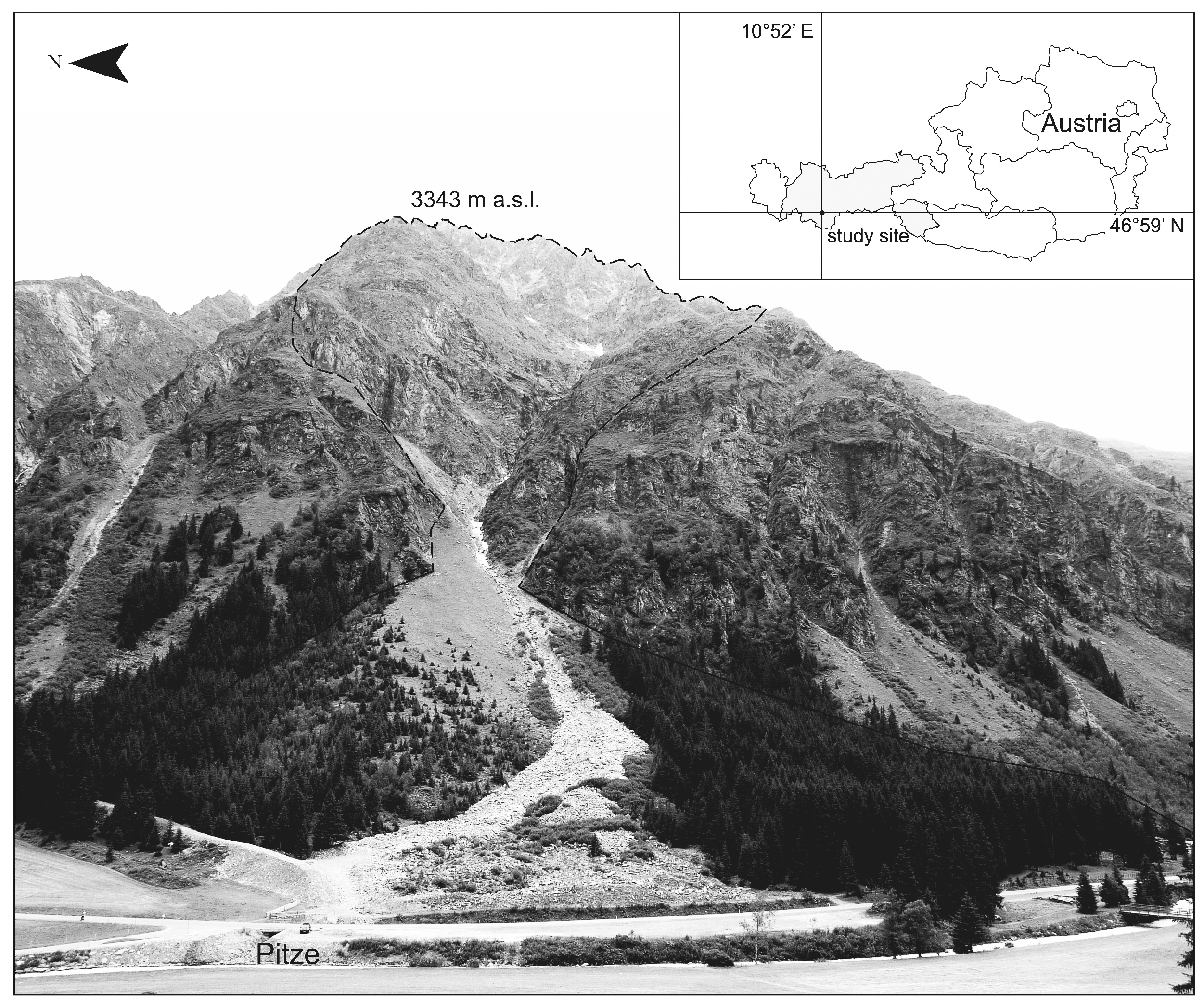
2. Study Area
3. Method
3.1. Numerical Modelling
3.2. Modelling Background
3.3. Evaluation and Validation
3.4. Sensitivity Analysis
4. Results and Discussion
4.1. Back-Analysis of the Event
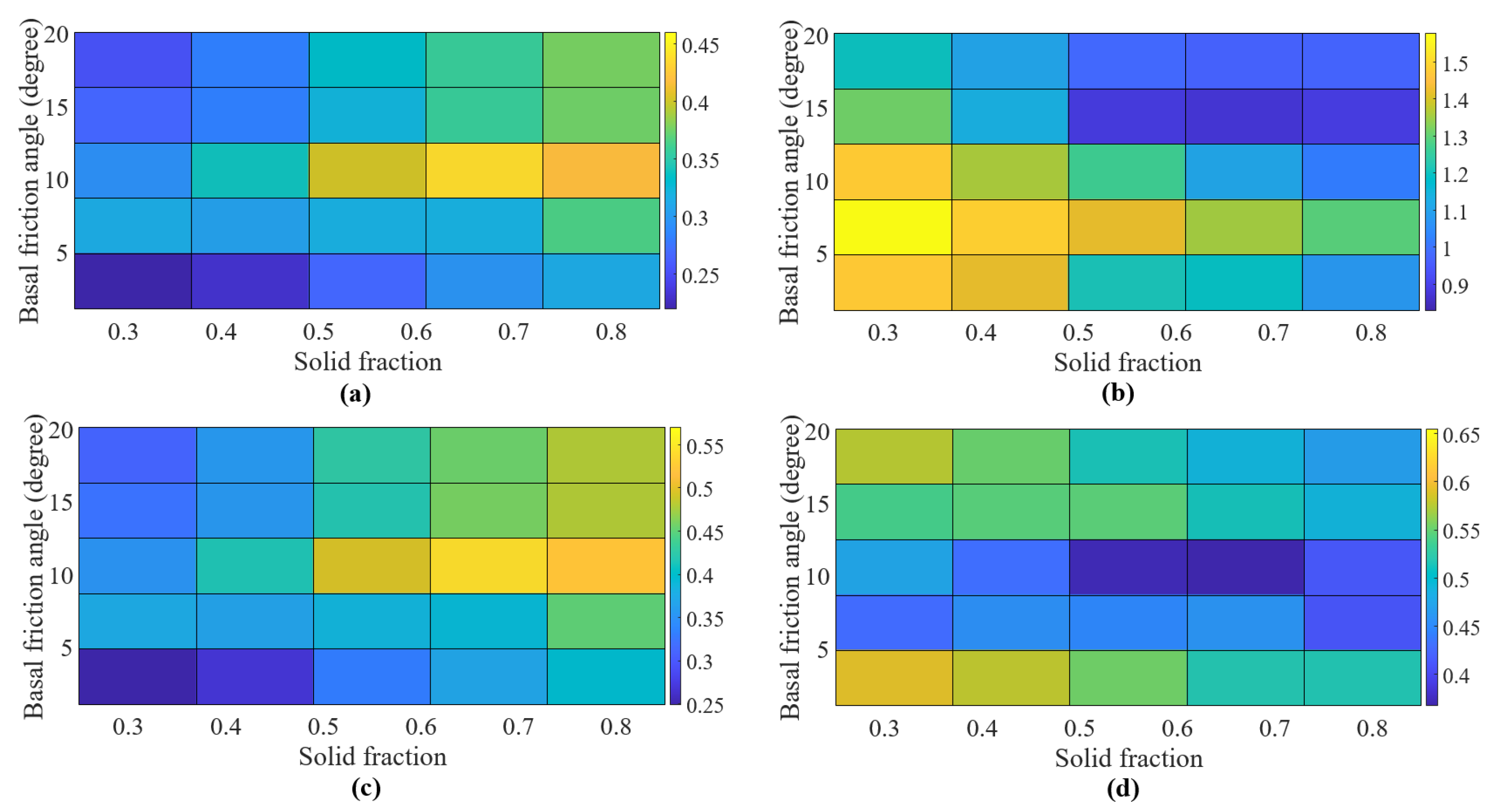
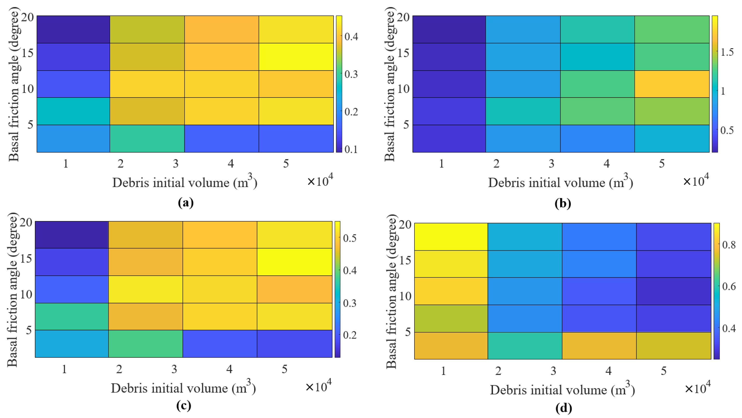
4.2. Results of the Sensitivity Analysis
5. Concluding Remarks
Author Contributions
Funding
Data Availability Statement
Acknowledgments
Conflicts of Interest
References
- Yune, C.Y.; Chae, Y.K.; Paik, J.; Kim, G.; Lee, S.W.; Seo, H.S. Debris flow in metropolitan area—2011 Seoul debris flow. J. Mt. Sci. 2013, 10, 199–206. [Google Scholar] [CrossRef]
- Dowling, C.A.; Santi, P.M. Debris flows and their toll on human life: A global analysis of debris-flow fatalities from 1950 to 2011. Nat. Hazard. 2014, 71, 203–227. [Google Scholar] [CrossRef]
- Ren, D. The devastating Zhouqu storm-triggered debris flow of August 2010: Likely causes and possible trends in a future warming climate. J. Geophys. Res. Atmos. 2014, 119, 3643–3662. [Google Scholar] [CrossRef]
- Langdon, S.; Johnson, A.; Sharma, R. Debris flow syndrome: Injuries and outcomes after the Montecito debris flow. Am. Surg. 2019, 85, 1094–1098. [Google Scholar] [CrossRef] [PubMed]
- Scheidegger, A.E. On the prediction of the reach and velocity of catastrophic landslides. Rock Mech. 1973, 5, 231–236. [Google Scholar] [CrossRef]
- Rickenmann, D. Empirical relationships for debris flows. Nat. Hazard. 1999, 9, 47–77. [Google Scholar] [CrossRef]
- Legros, F. The mobility of long-runout landslides. Eng. Geol. 1999, 63, 301–331. [Google Scholar] [CrossRef]
- Scheidl, C.; Dieter, R. Empirical prediction of debris-flow mobility and deposition on fans. Earth Surf. Process. Landforms 2010, 35, 157–173. [Google Scholar] [CrossRef]
- Savage, S.B.; Hutter, K. The motion of a finite mass of granular material down a rough incline. J. Fluid Mech. 1989, 199, 177–215. [Google Scholar] [CrossRef]
- Hungr, O. A model for the runout analysis of rapid flow slides, debris flows, and avalanches. Can. Geotech. J. 1995, 32, 610–623. [Google Scholar] [CrossRef]
- Pudasaini, S.; Columban, H. Rapid shear flows of dry granular masses down curved and twisted channels. J. Fluid Mech. 2003, 495, 193–208. [Google Scholar] [CrossRef]
- Bagnold, R.A. Experiments on a gravity-free dispersion of large solid spheres in a Newtonian fluid under shear. Proc. R. Soc. Lond. Ser. Math. Phys. Sci. 1954, 225, 49–63. [Google Scholar]
- Voellmy, A. Uber die zerstorungskraft von lawinen. Schweiz. Bauztg. 1955, 73, 159–162. [Google Scholar]
- Iverson, R.M.; Denlinger, R.P. Flow of variably fluidized granular masses across three-dimensional terrain. J. Geophys. Res. Solid Earth 2001, 106, 553–566. [Google Scholar]
- Pitman, E.B.; Le, L. A two-fluid model for avalanche and debris flows. Philos. Trans. R. Soc. Lond. Ser. 2005, 363, 1573–1601. [Google Scholar] [CrossRef] [PubMed]
- Mergili, M.; Fischer, J.T.; Krenn, J.; Pudasaini, S.P. r.avaflow v1, an advanced open-source computational framework for the propagation and interaction of two-phase mass flow. Geosci. Model Dev. 2017, 10, 553–569. [Google Scholar] [CrossRef]
- Pudasaini, S.P.; Mergili, M. A multi-phase mass flow model. J. Geophys. Res. Earth Surf. 2019, 124, 2920–2942. [Google Scholar] [CrossRef]
- Naqvi, M.W.; KC, D.; Hu, L. Numerical modeling and a parametric study of various mass flows based on a multi-phase computational framework. Geotechnics 2022, 2, 506–522. [Google Scholar] [CrossRef]
- Mergili, M.; Bernhard, F.; Jan-Thomas, F.; Christian, H.; Shiva, P.P. Computationale experiments on the 1962 and 1970 landslide events at Huascaran (Peru) with r.Avaflow: Lessons learned for predictive mass flow simulations. Geomorphology 2018, 322, 15–28. [Google Scholar] [CrossRef]
- Mergili, M.; Jaboyedoff, M.; Pullarello, J.; Pudasaini, S.P. Back calculation of the 2017 piz cengalo-bondo landslide cascade with r.avaflow: What we can do and what we can learn. Nat. Hazards Earth Syst. Sci. 2020, 20, 505–520. [Google Scholar] [CrossRef]
- Kogelnig-Mayer, B.; Markus, S.; Michelle, S.B.; Johannes, H.; Florian, R.M. Possibilities and limitations of dendrogeomorphic time-series reconstructions on sites influenced by debris flows and frequent snow avalanche activity. Arctic Antarct. Alp. Res. 2011, 43, 649–658. [Google Scholar] [CrossRef]
- Schraml, K.; Thomschitz, B.; McArdell, B.W.; Graf, C.; Kaitna, R. Modeling debris-flow runout patterns on two alpine fans with different dynamic simulation models. Nat. Hazards Earth Syst. Sci. 2015, 15, 1483–1492. [Google Scholar] [CrossRef]
- Pudasaini, S.P. A general two-phase debris flow model. J. Geophys. Res. Earth Surf. 2012, 117. [Google Scholar] [CrossRef]
- Pszonka, J.; Schulz, B.; Sala, D. Application of mineral liberation analysis (MLA) for investigations of grain size distribution in submarine density flow deposits. Mar. Pet. Geol. 2021, 129, 105109. [Google Scholar] [CrossRef]
- Pszonka, J.; Schulz, B. SEM Automated Mineralogy applied for the quantification of mineral and textural sorting in submarine sediment gravity flows. Gospod. Surowcami Miner. Miner. Resour. Manag. 2022, 38, 105–131. [Google Scholar]
- European Commission. The Official Portal for European Data. Available online: https://data.europa.eu/data/datasets/0454f5f3-1d8c-464e-847d-541901eb021a?locale=en (accessed on 15 January 2020).
- Calligaris, C.; Zini, L.; Calligaris, C.; Zini, L. Debris flow phenomena: A short overview? In Earth Sciences; Dar, I.A., Ed.; Intechopen: London, UK, 2012; pp. 71–89. [Google Scholar]
- Iverson, R.M. Debris flows: Behaviour and hazard assessment. Geol. Today 2014, 30, 15–20. [Google Scholar] [CrossRef]
- Turnbull, B.; Bowman, E.T.; McElwaine, J.N. Debris flows: Experiments and modelling. C.R. Phys. 2015, 16, 86–96. [Google Scholar] [CrossRef]
- Wang, Z.-Y.; Lee, J.H.W.; Melching, C.S. Debris flows and landslides. In River Dynamics and Integrated River Management; Springer: Berlin/Heidelberg, Germany, 2015; pp. 193–264. [Google Scholar]
- Thouret, J.C.; Antoine, S.; Magill, C.; Ollier, C. Lahars and debris flows: Characteristics and impacts. Earth Sci. Rev. 2020, 201, 103003. [Google Scholar] [CrossRef]
- Coe, J.A.; David, A.K.; Jonathan, W.G. Conditions for debris flows generated by runoff at Chalk Cliffs, central Colorado. Geomorphology 2008, 96, 270–297. [Google Scholar] [CrossRef]
- Coe, J.A.; Jason, W.K.; Scott, W.M.; Dennis, M.S.; Thad, A.W. Chalk Creek Valley: Colorado’s natural debris-flow laboratory. GSA Field Guid. 2010, 18, 95–117. [Google Scholar]
- Formetta, G.; Giovanna, C.; Pasquale, V. Evaluating performance of simplified physically based models for shallow landslide susceptibility. Hydrol. Earth Syst. Sci. 2016, 20, 4585–4603. [Google Scholar] [CrossRef]
- Simons, D.B.; Richardson, E.V. The Effect of Bed Roughness on Depth-Discharge Relations in Alluvial Channels; USGS Water Supply Paper 1498-E; USGS: Reston, VA, USA, 1962. [Google Scholar]
- Giraud, R.E.; Castleton, J.J. Estimation of Potential Debris-Flow Volumes for Centerville Canyon, Davis County, Utah; Utah Geological Survey: Salt Lake City, UT, USA, 2009. [Google Scholar]
- Walter, F.; Amann, F.; Kos, A.; Kenner, R.; Phillips, M.; de Preux, A.; Huss, M.; Tognacca, C.; Clinton, J.; Diehl, T.; et al. Direct observations of a three million cubic meter rock-slope collapse with almost immediate initiation of ensuing debris flows. Geomorphology 2000, 351, 106933. [Google Scholar] [CrossRef]
- Diwakar, K.C.; Dangi, H.; Naqvi, M.W.; Kadel, S.; Hu, L.-B. Recurring landslides and debris flows near Kalli Village in the Lesser Himalayas of Western Nepal. Geotech. Geol. Eng. 2023, 41, 3151–3168. [Google Scholar] [CrossRef]
- Rom, J.; Haas, F.; Hofmeister, F.; Fleischer, F.; Altmann, M.; Pfeiffer, M.; Heckmann, T.; Becht, M. Analysing the large-Scale debris flow event in July 2022 in Horlachtal, Austria using remote sensing and measurement data. Geosciences 2023, 13, 100. [Google Scholar] [CrossRef]
- Kean, J.W.; McCoy, S.W.; Tucker, G.E.; Staley, D.M.; Coe, J.A. Runoff-generated debris flows: Observations and modeling of surge initiation, magnitude, and frequency. J. Geophys. Res. Earth Surf. 2013, 118, 2190–2207. [Google Scholar] [CrossRef]
- Hungr, O.; Evans, S.G.; Bovis, M.J.; Hutchinson, J.N. A review of the classification of landslides of the flow type. Environ. Eng. Geosci. 2001, 7, 221–238. [Google Scholar] [CrossRef]
- Iverson, R.M. The physics of debris flows. Rev. Geophys. 1997, 35, 245–296. [Google Scholar] [CrossRef]


| Parameters | Definition | Range | Theoretical Optimum |
|---|---|---|---|
| Critical success index (CSI) | [0, 1] | 1 | |
| Factor of conservativeness (FOC) | [0, ∞] | 1 | |
| Heidke skill score (HSS) | [, 1] | 1 | |
| Distance to perfect classification (D2PC) | ; | [0, 1] | 0 |
| Parameter | Symbol | Value |
|---|---|---|
| Solid | ||
| Density | 2840 | |
| Internal Friction Angle | ||
| Basal Friction Angle | ||
| Drag Coefficient | 0.02 | |
| Fluid | ||
| Density | 1000 | |
| Kinematic Viscosity | 0.001 | |
| Fluid friction coefficient | c | 0.08 |
| Validation Parameter | Value |
|---|---|
| CSS | 0.464 |
| FOC | 1.004 |
| HSS | 0.574 |
| D2PC | 0.373 |
Disclaimer/Publisher’s Note: The statements, opinions and data contained in all publications are solely those of the individual author(s) and contributor(s) and not of MDPI and/or the editor(s). MDPI and/or the editor(s) disclaim responsibility for any injury to people or property resulting from any ideas, methods, instructions or products referred to in the content. |
© 2023 by the authors. Licensee MDPI, Basel, Switzerland. This article is an open access article distributed under the terms and conditions of the Creative Commons Attribution (CC BY) license (https://creativecommons.org/licenses/by/4.0/).
Share and Cite
Naqvi, M.W.; Kc, D.; Hu, L. Numerical Modelling and Sensitivity Analysis of the Pitztal Valley Debris Flow Event. Geosciences 2023, 13, 378. https://doi.org/10.3390/geosciences13120378
Naqvi MW, Kc D, Hu L. Numerical Modelling and Sensitivity Analysis of the Pitztal Valley Debris Flow Event. Geosciences. 2023; 13(12):378. https://doi.org/10.3390/geosciences13120378
Chicago/Turabian StyleNaqvi, Mohammad Wasif, Diwakar Kc, and Liangbo Hu. 2023. "Numerical Modelling and Sensitivity Analysis of the Pitztal Valley Debris Flow Event" Geosciences 13, no. 12: 378. https://doi.org/10.3390/geosciences13120378