1. Introduction
The global sea level has risen about 20 cm in the last century [
1,
2], and Intergovernmental Panel on Climate Change (IPCC) projections show an expedited increase in the global mean sea level (GMSL) [
3,
4,
5]. The accelerated sea level rise is mainly due to the thermal expansion of seawater and the recession of glaciers from melting attributed to climate change. The modeling and prediction of sea level rise is a challenging problem due to the complexity of climate and environmental factors impacting sea level changes. The latest GMSL rise estimate is about 3 mm/year, which does not represent the sea level variations in localized areas. In Florida, there are 8436 miles of coastline, all of which are directly affected by sea level rise. Displacement, infrastructure, and city planning, along with rapid population growth, make it imperative to gain a better understanding of sea level rise in this area.
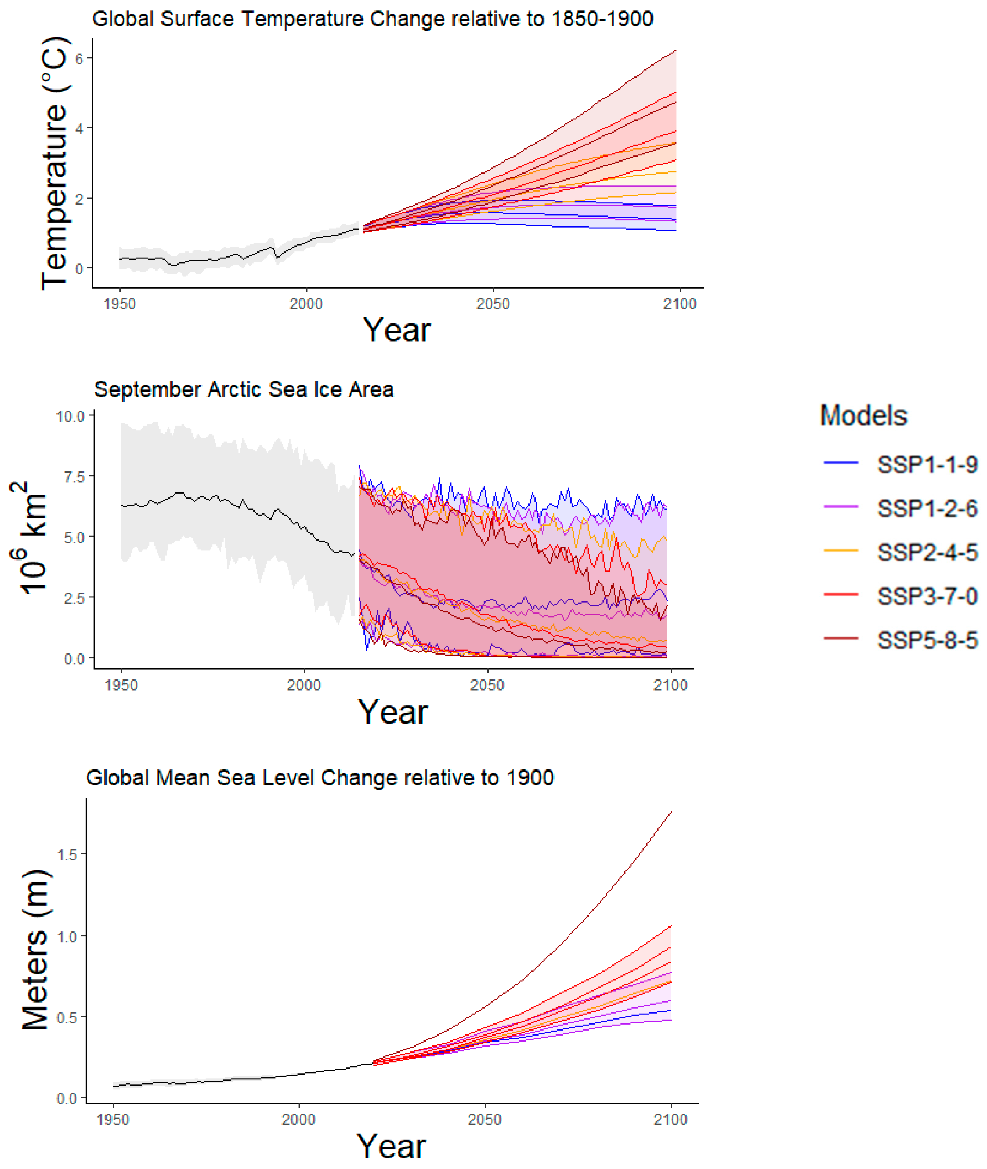
GMSL, Global Surface Temperature Changes (GSTC) relative to 1850–1900, and the September Arctic Sea Ice Area (SASIA) are depicted in
Figure 1. GMSL has risen between 16 and 21 cm within the last century [
1,
2] and will likely accelerate in the future. For example, projections by the IPCC depicted in
Figure 1 indicate that the global mean sea level may increase up to 1 m by 2100 [
3,
4,
5]. The projections represent five different scenarios of Shared Socio-economic Pathways (SSPs) based on four factors including sustainable development, regional competition, inequality, and fossil-fuel consumption [
4].
The primary cause of the global increase in sea level can be attributed to climate change through the thermal expansion of seawater and the recession of glaciers from melting [
6,
7]. However, estimating local and regional sea level rise is a difficult task because of the complexity of climate and environmental factors that influence its change. The latest global mean sea level rise estimate indicates that it has increased to about 3.7 mm/year (for the period 2006–2018,
Figure 1) [
8,
9]. However, this rate has considerable local and regional variability that depends on both environmental and climate factors [
8,
10].
Given its extensive shoreline and large coastal population, Florida is of particular concern with respect to SLR. Hence, it is essential to discern whether or not SLR trends in Florida are consistent with the global rates. The Florida coastline comprises two ocean basins, the Atlantic and the Gulf of Mexico (GOM). In addition, the landmass of Florida is sinking, which increases the threat of local flooding especially during high impact events such as tropical cyclones. GMSL is projected to rise between 0.3 and 0.7 m by 2060 relative to 1850–1900, depending on the SSP [
3,
4]. Approximately two-thirds of the global coastline is projected to have regional SLR within +/−20% of the global mean increase (
Figure 1). Hence, even for midrange GMSL projections (i.e., on the order of 0.75 m by 2100) this represents a substantial difference of about 30 cm. The localization of projected SLR is an active and challenging area of research [
11,
12,
13,
14,
15,
16,
17]. This process typically involves observations from in situ tide gauges and satellite altimetry, which can be used to evaluate and/or calibrate GCM projections.
Previous sea level studies in Southeastern United States suggest that temperature, salinity, and El Niño are relevant factors in this region [
18]. Large-scale weather patterns (winds) can also help to explain some of the observed (decadal) variability in coastal sea level. Furthermore, a number of recent studies indicate that global SLR has accelerated during the past several decades [
19,
20,
21]. The implications of SLR on the region and the direct threat that it poses to populated coastal areas are significant. In particular, there are 8436 miles of vulnerable coastline that is susceptible to flooding in Florida while, according to the US Census, 16 million Floridians—or three-quarters of the state’s population—live in coastal counties. Florida’s population growth ranked second in the nation—adding almost a quarter of a million residents in 2021. However, despite the increasing threat to coastal infrastructure and population, Florida sea level studies are a decade old [
3,
18,
22,
23,
24].
The objectives of this study are to (1) compare estimates of local sea level rise along the Florida coastline with the global estimates of sea level rise and to (2) model the sea level in coastal Florida using climate factors. A schematic of the proposed work is depicted in
Figure 2, demonstrating the required tasks from data collection to modeling. Satellite altimetry and climate factors including water temperature, water salinity, El Niño southern oscillation, and basin-scale sea level trends are collected to implement a predictive model of sea level at selected tide gauge locations along the Florida coast. The local rates of sea surface height were compared to regional and global measurements, and the sea level changes across coastal Florida were then modeled using both parametric and nonparametric methods.
2. Data Description
The focus of this study corresponds to the altimetry record that extends about three decades beginning in 1992 and comprises a series of four satellites (TOPEX/Poseidon, Jason-1, Jason-2, and Jason-3) [
25]. For this study, gridded SSHA data on a 1/6th degree grid and 5-day intervals were extracted from the NASA PODAAC server [
26]. The anomalies are derived from a spatiotemporal mean map of SSH, which is computed using the average of the grids from all available years (1992–2019), then subtracted from individual grid values (the new data) to estimate the sea surface height anomalies. The SSHA (
Figure 3) are corrected for an inverse barometer effect [
27] but are not adjusted for isostasy effects (ocean deepening), which increase global rates of sea level change on the order of 0.3 mm/year [
28]. Also, altimeter data near the coast are prone to error from land contamination of the radiometer, tidal impacts, and data interpolation issues [
26]. Hence, direct comparison with the tide gauges is important. The tide gauge data were obtained from the Permanent Service for Mean Sea Level (PSMSL) web interface (Holgate et al., 2013; PSMSL, 2023). Based on the analysis of sea-level pressure data, atmospheric pressure changes have been reported to not have any significant trend [
29], and numerous studies of GMSL using tide gauges applied no corrections for the inverted barometer effect as this correction is small on century time scales [
30].
Two environmental factors, water temperature and salinity (Practical Salinity Units, PSU), were obtained from the Estimating the Circulation and Climate of the Ocean (ECCO) Version 4 Release 4 (R4) providing the latest ocean state estimate product [
31,
32,
33]. The simulations were performed using the Massachusetts Institute of Technology general circulation model (MITgcm). When available, the model output has been fit to in situ and satellite observations (sea level, sea ice, temperature/salinity profiles, SST, dynamic topography) using linear regression [
34]. The gridded output is available at depth (50 levels) to about 6000 m. However, only the uppermost model level (5 m depth) is used here. Temperature and salinity are important as they impact both sea level and ocean circulation. The horizontal resolution varies spatially from 22 to 110 km, with the resolution increasing in high latitudes. The ECCO temperature and salinity data depict variability along the Florida coastline (
Figure 4).
El Niño has both global and regional impacts on sea level. El Niño or La Niña events are defined when the El Niño 3.4 SST anomalies exceed +/−0.5C for a period of 5 months or more. At large scales, precipitation is reduced over land, and there is less evaporation over the ocean, which increases the GMSL. El Niño can also have a significant impact on the regional weather. For example, in the SE US, it affects the genesis region and path of extratropical cyclones over the eastern GOM by shifting the Northern Hemisphere storm tracks toward the equator and downstream [
35,
36,
37]. As a result, coastal sea level variability in the northern and eastern GOM tends to increase (October to March) with extreme sea level anomalies occurring during the ENSO warm phase [
38]. Factors responsible for the variability include increased runoff from land-based precipitation, sea level pressure anomalies, and winds [
36]. Here, the ENSO 3.4 index is used to account for the effects of El Niño events in the statistical modeling. The data (available at
https://psl.noaa.gov/gcos_wgsp/Timeseries/Data/nino34.long.data (accessed on 26 June 2021)) comprise a monthly timeseries from 1870 to 2020, based on sea surface temperature anomalies over the equatorial Pacific from 5N to 5S and 120 to 170W.
Tide Gauges Versus Altimetry
Using the SSHA at the nearest altimetry grid point, the SLR trends (1993–2019) were calculated and compared with in situ tide gauges at 15 Florida locations (
Figure 5). Altimetry and tide gauge values for 15 Florida locations in this study along with the absolute percentage error are listed in
Table 1. Due to the satellite land mask, the two are not co-located with nearest neighbor distances varying from 4 km to 40 km (with an average separation of approximately 16 km). In order to compare with the PSMSL data, the SSHA were upscaled to monthly averages. In general, the trends are higher for the tide gauges at all but three locations (Apalachicola, Naples, and Fernandina Beach). The differences are small at both Naples and Apalachicola (0.1 and 0.3 mm/yr, respectively), while the altimeter rates are substantially higher with respect to Fernandina Beach (2.2 mm/yr). The tide gauge trends at both Fernandina and Mayport (located close to each other) are relatively low (2.8 and 3.5 mm yr
−1, respectively). However, the SLR rates are quite high for the Lake Worth tide gauge (7.2 mm yr
−1, beginning in 2010) and the altimetry (8.8 mm yr
−1) for the overlapping period of 2010–2019. Because of the relatively short time series, Lake Worth was excluded from the linear regression. Fernandina Beach was an outlier and hence was excluded (the tide gauge is tucked inside an inlet near the confluence of the St. Mary’s and Amelia rivers). The regression yields an R
2 value of 0.49, an intercept of 2.55 mm yr
−1, and a slope of 0.55. The discrepancy between the gauge and altimeter decreases by increasing trends.
Because tide gauges actually record the sea level in situ, they are generally considered as more accurate for sea level measurements [
39]. However, a drawback of tide gauge measurements is that the changes in the sea surface are recorded relative to the land. Hence, in order to obtain a true sea level signal, vertical movements must be estimated to adjust the tide gauge measurements [
40].
3. Methods
Initially, multiple linear regression was used to model the sea level variations. Multiple regression is a parametric method that can be used to model a response (here, sea level rise) based on various predictors (and their potential interactions). The standard multiple regression assumes a simple form for the following:
where
Y is the response,
are
p predictors, and
are the coefficients of the predictors [
41]. Six factors, including the year, global SSHA, regional SSHA, water temperature, water salinity, ENSO, and each of their interactions were considered to model sea level rise.
Generalized additive model (GAM) was also used to model the sea level variations. GAM is a nonparametric model in which the response is modeled as the sum of the smoothed functions of the predictors [
42,
43,
44]. This adds substantial flexibility over multiple regression in modeling sea level variations because the trend of each predictor is separately modeled and added to discover the trend of the response. GAM is a generalization of the additive model defined with the following:
where
is the intercept, and
,
are smoothing functions [
43]. In the case of a single predictor, the model becomes the following:
where the constant term
is suppressed and placed into the function. The smoothing function
can be estimated from the data using a reasonable estimate of
. One way of estimating the expectation is by using nonparametric local average estimates:
where
is the estimator of the smoothing function,
is the
realization of
out of a total of
realizations,
is the neighborhood of
,
is the number of points in the neighborhood
of span
, and
is the average of
’s for
. The type of neighborhood considered here is the symmetric nearest neighborhood:
where
has
points, and it is assumed that
is odd. The neighborhood becomes truncated at the endpoints if there are not at least
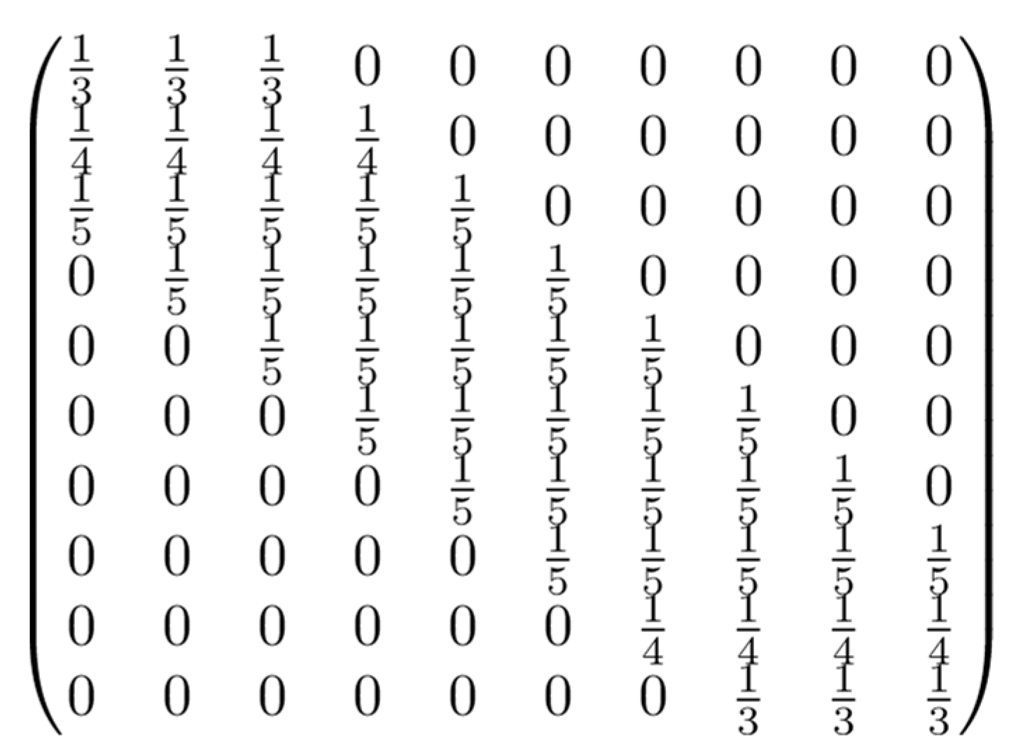
points available. This truncation is shown in the smoothing matrix in
Figure 6 where span
and
. In the first row, each of the points included only have a neighborhood of 3 points available. When the smoothing function is estimated using local averaging, large bias occurs at the endpoints. This bias is because of the truncation at the endpoints, as seen in
Figure 6. To address this, a parametric local linear regression can be used in place of the local averaging:
where
and
are the least-squares estimates for the points within
:
and
where
and
are the following:
The local linear regression estimate of the smoothing function is dependent on the neighborhood
. Shrinking the neighborhood causes the systemic or bias component of the estimation error to decrease, and increasing the neighborhood sample size will decrease the variance component of the error [
45]. The span size
of
has a large impact on the estimate. The value of the span should be between
and 2 to trade off the bias and variability of the estimate [
43,
44]. The neighborhood contains only
for
and
. This means the estimate will have a high variance, as each smoothed point will be equal to its corresponding
value and no smoothing will have occurred. When
,
becomes the global least-squares regression line, which means that the estimate may be biased. This is because
will contain all points. The estimate will be too smooth, as any curvature of the underlying function will not be included. A data-based criterion can be used to select the span of
if the estimates of
are considered as local minimizers of the integrated prediction squared error (PSE):
where
PSE is the squared error between the true response values and the smoothed predictor values.
Generalized additive models (GAM) draw from both the generalized linear model (GLM) and the additive model [
42,
44]. GAM generalizes the linear predictor,
Y, as the following:
where
is the systematic component of the model,
is the link function, and
, for
, are the smoot functions. The estimates for each
are found using nonparametric smoothers such as cubic splines or local (nonparametric) linear regression. The measurements used to analyze GAM in this study were the adjusted
R2 (
) and Akaike Information Criterion (AIC). The
is calculated with the following:
where
n is the total sample size, and
p is the number of independent variables. The
AIC is calculated with the following:
where
is the maximum likelihood value for the model, and
is the number of estimated variables [
32,
46]. Both
and AIC quantify goodness of fit, with a high (
) or low AIC signifying a model that fits the data well.
To provide visualizations for the GAM, graphical representations of the GAM were smoothed using loess. Loess is a type of smoothing function based on locally weighted polynomial regression in which the dependent variable is smoothed as a function of the independent variable(s). The estimate,
, provided by the loess smoother is a linear combination of the
where
depends on the predictors
[
47,
48].
Given the six potential predictors, there are 57 possible combinations to use in GAM. All of model variations were run separately at each of the 15 locations. For each of the 57 variations, both the adjusted R-squared and AIC values were averaged across all tested locations. The models were ranked from the highest to lowest average adjusted R-squared and then from the lowest to highest average AIC to identify the optimal model for all locations. After determining that the optimal model included the year as a predictor, the model was modified to exclude year as a factor for all locations to check if a less ambiguous model would fit the data just as well, since year is often considered a proxy variable for many environmental and climate factors.
4. Results
Examining the trend and variance of the SSSHA data in the initial analysis led to the confirmation that the global mean sea level (GMSL) rate is about 3 mm/year (not adjusted for isostacy), as seen in
Figure 7. Local sea level rise in Florida exceeds GMSL at 14 out of 15 of the selected locations and ranges from about 2.5 mm/year (Mayport) to about 5 mm/year (Apalachicola). Local variability ranges from about 2000 (Lake Worth) to about 6200 (Apalachicola)
and is greater than both regional and global variances.
First, multiple regression was used to model the sea level rise for the selected locations along the Florida coast. The full multiple regression model with all predictors is as follows:
where
is year,
is regional SSHA,
is global SSHA,
is ENSO,
is water temperature, and
is water salinity. The multiple regression model for Pensacola is depicted in
Figure 8 (top). The multiple regression model with the lowest average BIC of about −67 is as follows:
where the values
are the factors of the model. As seen in
Figure 8 (middle), the sea level data are fairly normal, and the multiple regression model provides a satisfactory fit. However, a nonlinear trend is visible in the residual plot (
Figure 8 (bottom)). Additionally, the model consisted only of interaction terms between variables. Hence, a nonparametric model, such as GAM, is more relevant to fit sea level data and was used for modeling the nonlinear trends in sea level changes. The best model is selected based on two goodness of fit criteria,
and AIC. All six predictors including year, global average, adjacent basin anomalies, water temperature, water salinity, and ENSO 3.4 Index were identified as significant predictors in the selected GAM. This model will be abbreviated as SLR-M1 (sea level rise model 1), standing for year, adjacent basin SSHA, global SSHA, ENSO, salinity, and temperature.
The average
value for the selected locations was 0.86, with the lowest value of 0.70 for Mayport and the highest value of 0.95 for Pensacola (
Table 2). The average AIC value for the SLR-M1 model at each selected location was −137.61, with the highest being −115.62 for Mayport and the lowest value of −159.05 for Pensacola (
Table 2). The fitted model using GAM from Lake Worth, FL with
of 0.85 and AIC of −139.09 is depicted in
Figure 9 (Top Left). The assumptions for whether or not the conditions for this model are met at that particular location are shown in
Figure 9 (Top Right) and (Bottom).
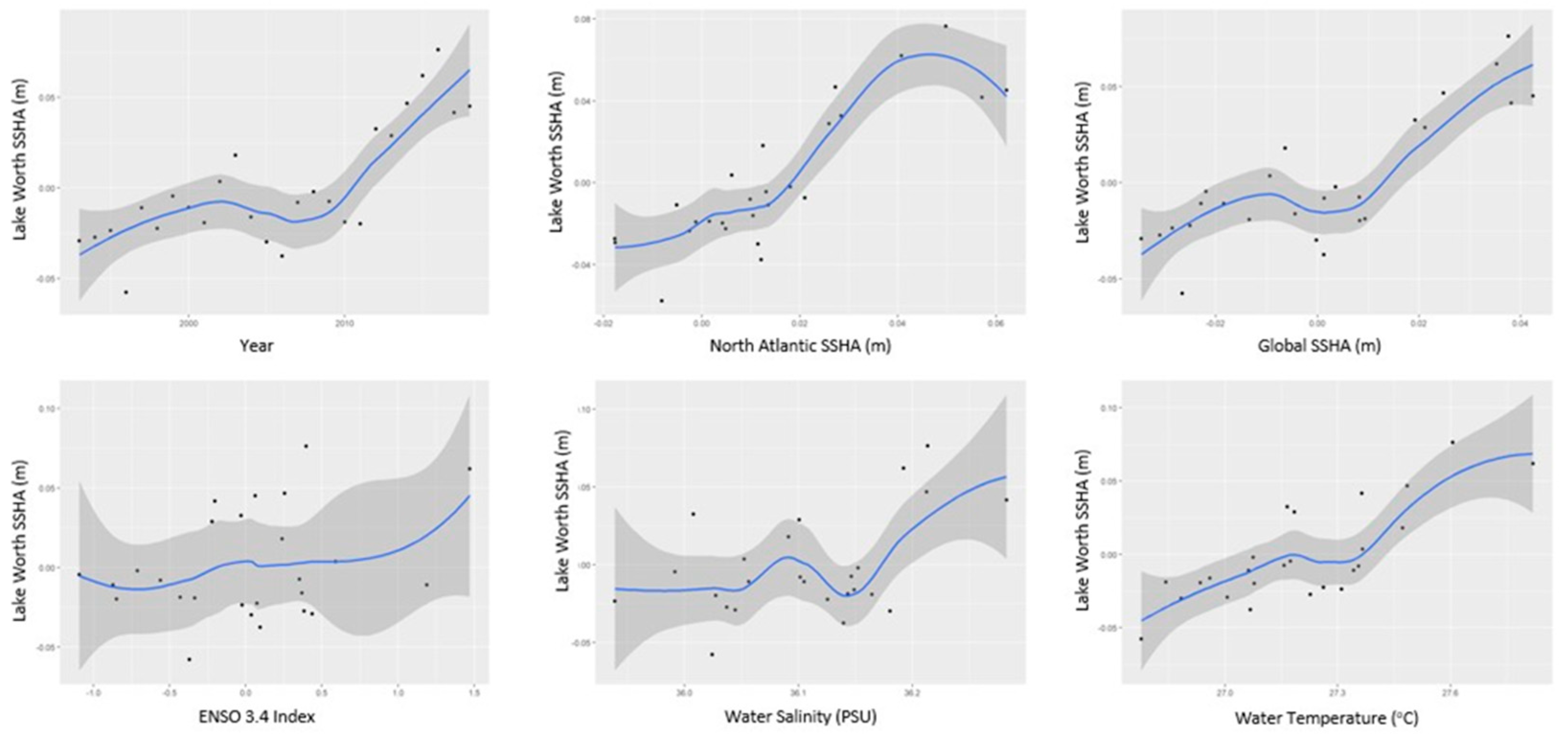
The fitted SLR-M1 GAM model to sea level data at Lake Worth, FL versus each predictor is depicted in
Figure 10 (black diamonds). The smoothed trend of each predictor is obtained using loess (blue line). While the year does partially represent time, it is mostly a proxy variable that includes other factors that may influence sea level change. Due to this, we looked at a GAM that did not include year as a predictor. This new model will be abbreviated as SLR-M2 (sea level rise model 2), standing for adjacent basin SSHA, global SSHA, ENSO, salinity, and temperature. The adjusted R-squared values were lower (on average) for all tested locations, with an average of 0.83, and the AIC values were on average higher for all tested locations, with an average of −134.07 (
Table 3). However, this model is less ambiguous due to the omission of year as a predictor. The smoothed predictor functions for this model fitted at Lake Worth, FL are shown in
Figure 11.
Figure 12 shows a matrix of the response of the SLR-M2 model at every tested Florida location in which the sea surface height anomalies (m) are modeled using the sum of functions of the predictors. It is important to note that all but four of the locations show an increasing trend for SSHA. Due to the sparseness of data points on the right side of the plots, the gray confidence intervals widen, and some prediction clarity is lost. Hence, predictions with a relatively high sum of predictions should be made with caution. Since the SLR-M2 model does not account for time, this is indicative of the fact that while sea level is increasing in Florida over time, time is not the only factor contributing to sea level rise.
Figure 13 shows a comparison between the SLR-M2 GAM predicted SSHA and the observed SSHA plotted as a function of time. For some of the locations, such as Pensacola, FL in
Figure 13a, the trend was very different for each of these two plots. This validates the fact that the increasing/decreasing trends of SSHA are due to predictors other than year in the SLR-M2 GAM. For other locations, such as Virginia Key, FL in
Figure 13b, the trends for both plots were similar. This shows that sea level increases due to the other predictors having a similar pattern to sea level rise over time.
A matrix where the SSHA for each of the Florida locations was plotted as a function of time is depicted in
Figure 14. All of these plots in the matrix show an increasing trend in sea level rise. This is a good indicator that there is an overall increasing trend of rising sea levels in Florida. However, both the SLR-M1 GAM and the SSHA time series depicted in
Figure 14 seem to show that the increase in sea levels in coastal Florida becomes more severe as time progresses.
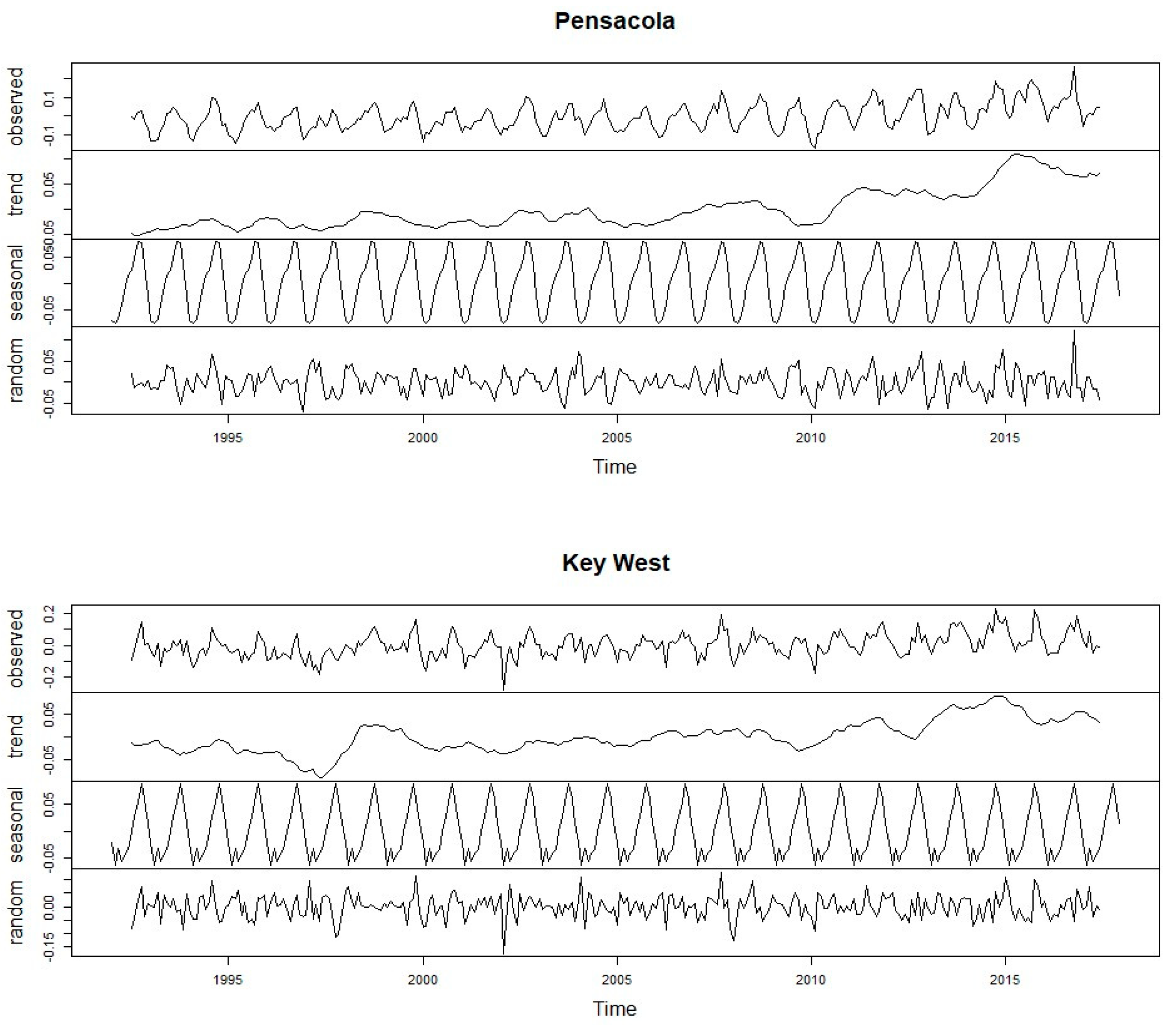
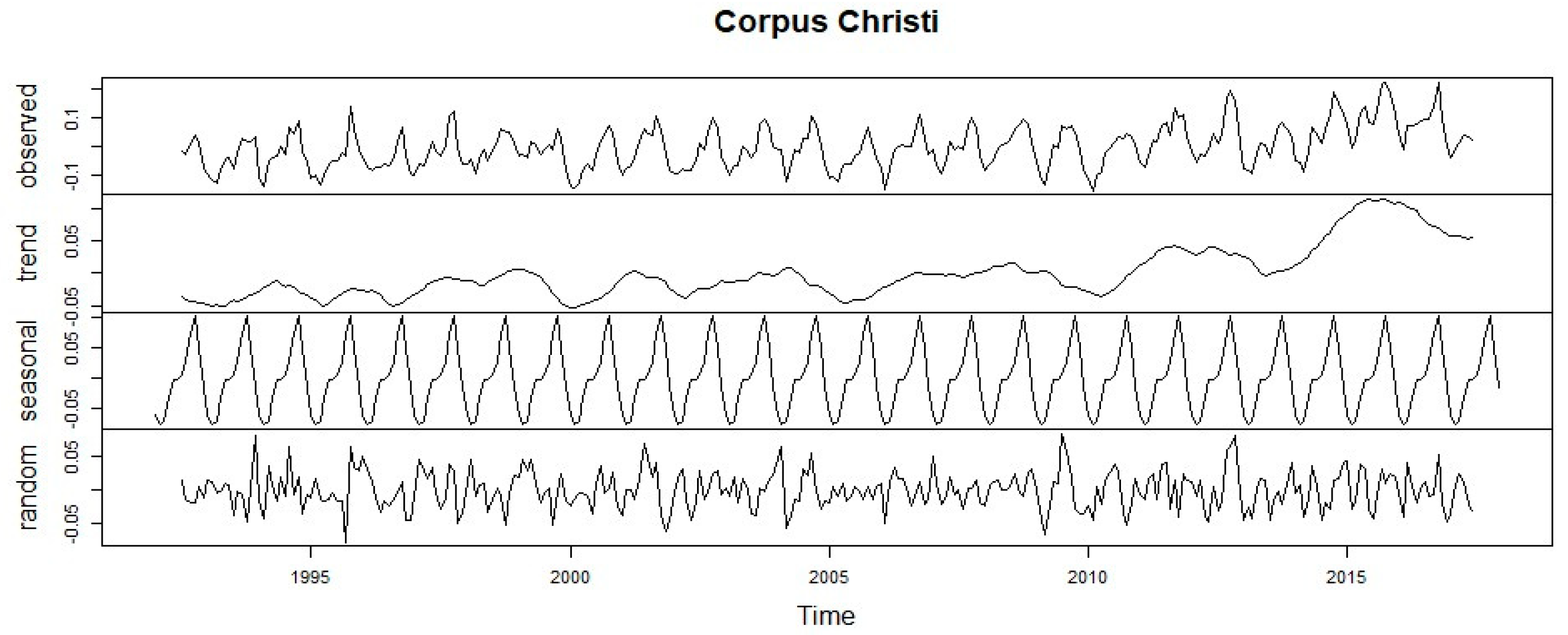
Figure 15 shows the altimetry data from three tide gauge stations. These stations were compared to each other to demonstrate the difference in sea level rise trends in Florida and in Texas. The
decompose () function in R was used to decompose the altimetry data into trend, seasonal, and random components. An additive model is used to construct the different components from the altimetry data. The trend component is constructed using a moving average of the observed data. The seasonal component was constructed by averaging the data. The random component is what is left over after removing the trend and seasonal components from the observed data. The locations chosen for this comparison were Pensacola, FL (
Figure 15 (top)), Key West, FL (
Figure 15 (middle)), and Corpus Christi, TX (
Figure 15 (bottom)). Pensacola is the closest tide gauge station to Corpus Christi, and Key West is another Florida location used to compare to Corpus Christi.
For each of the tide gauge locations, there is an increasing trend over time. It can be seen that the Pensacola and Corpus Christi trends are similar, whereas the Key West trend has less fluctuations with an overall increasing trend. Pensacola and Corpus Christi show increasing trends after 2010, but this is not visible in Key West. However, all locations show similar trends from 2010.
5. Discussion
The global sea level has risen between 16 and 21 cm within the last century. It is predicted that this rate will be accelerated into the future due to climate change. The primary causes of this increase in sea level can be attributed to the thermal expansion of seawater and the recession of glaciers from melting. Projections from the IPCC show the global mean sea level rise may increase up to 1 m by 2100. Yet, obtaining accurate estimation of sea level rise is challenging because of the complexity of climate and environmental factors. The latest GMSL rise estimate is about 3 mm/year that sums up to 231 mm by 2100. However, this estimate does not represent changes in local areas. In Florida, there are 8436 miles of coastline, all of which is directly affected by sea level rise. Displacement, infrastructure, and city planning, along with rapid population growth, make it imperative to gain a better understanding of sea level rise in this area.
In this study, a model of sea level rise that takes into account altimetry, water temperature, water salinity, and El Niño southern oscillation (ENSO) 3.4 index for coastal Florida was proposed. The local rates and variances of sea surface height anomalies (SSHA) were analyzed and compared to regional and global measurements. The sea level changes across coastal Florida were modeled using both multiple regression and GAM. Both the SLR-M1 GAM and the SLR-M2 GAM show that water temperature, salinity, and ENSO 3.4 are all relevant factors for predicting sea level change in Florida. Alongside the significance of the climate and environmental factors, all of the Florida stations have an increasing trend in sea level rise (
Figure 14). This suggests that the Florida coast has a greater rate of sea level rise than the global mean sea level rise. The climate and environmental factors in the model signify a relationship between local sea level rise and climate change. Due to the accelerating climate change effects, the SLR-M1 GAM suggests that the local sea level rise will also accelerate. The SLR-M2 GAM also suggests that time is not the driving factor behind sea level rise. As seen in
Figure 12, most of the GAMs for the coastal Florida locations have an increasing trend in sea level rise. This indicates that the climate and environmental factors are contributing to the increasing rate of sea level rise.
The SLR—M1 GAM and SLR—M2 GAM also show that regional and global SSHA contribute to local sea level changes. Sea level changes in larger-scale systems are reflected in the sea level changes in smaller-scale systems and can be used to improve predictions for those smaller systems. Although local variations are comparable across coasts, the local sea level variations are higher than both regional and global variations (
Figure 7). This indicates that there is more variability in sea level rise on the local level than there is on a larger scale.
6. Conclusions
While global estimates for sea level rise provide a general trend that can be used in planning and policy making [
4], local estimates would provide more accurate estimates to prepare and plan. Additionally, there is a noticeable jump in the trend across all Florida locations in 2011 (
Figure 14) that is not present in other nearby geographical locations (for example, Corpus Christi, TX,
Figure 15 (bottom)). Due to its relative recency, this jump has not been extensively covered by previous climate change reports in the region. Further investigation of the sea level change in this period in the Florida region would be helpful for understanding additional factors that could lead to rising sea levels in the state and would contribute to the body of knowledge on sea level rise in the general southeastern region of the United States.
Factors such as average monthly winds, atmospheric pressures, and coastal currents have been found to be significant in sea level changes based on previous studies [
41]. Hence, to improve the proposed models in this study, additional climate and environmental factors will be considered in our future work. Moreover, using tide gauge data as “ground truth”, in addition to the altimetry data, would provide a more accurate SSHA model [
46,
49]. The 15 locations along the Florida coast were selected specifically so that this study can be replicated with tide gauge data. Repeating this study with tide gauges would also align the results with previous sea level reports from Florida.


 ,
, 


