Article

Back-Analysis of the Abbadia San Salvatore (Mt. Amiata, Italy) Debris Flow of 27–28 July 2019: An Integrated Multidisciplinary Approach to a Challenging Case Study

1
Department of Earth Sciences, University of Florence, 50121 Florence, Italy
2
Dipartimento di Scienze Fisiche, della Terra e dell’Ambiente, Università degli Studi di Siena, 53100 Siena, Italy
3
Department of Civil, Environmental and Mechanical Engineering, University of Trento, 38123 Trento, Italy
*
Author to whom correspondence should be addressed.
Geosciences 2022, 12(10), 385; https://doi.org/10.3390/geosciences12100385
Submission received: 30 June 2022 / Revised: 7 October 2022 / Accepted: 13 October 2022 / Published: 17 October 2022
(This article belongs to the Special Issue Scientific Assessment of Recent Natural Hazard Events)

Abstract

:
On 27–28 July 2019, in a catchment of the Mt. Amiata area (Italy), an extreme rainfall induced a debris flow, which caused a channeled erosive process just upstream of the Abbadia San Salvatore village, the obstruction of a culvert at the entrance to the urban area, and the subsequent flooding of the village. In this paper, we present the back analysis of this event. The complexity of this case study is due to several peculiar characteristics, but above all, to the clogging of the culvert, a phenomenon difficult to simulate numerically. The methodology used for the reconstruction of the event is based on a multidisciplinary approach. A geological field investigation was carried out to characterize the catchment and assess the availability of debris. Then, a cascade of numerical models was employed to reconstruct the debris flow: the FLO-2D software was used to model the runoff along the hydrographic network while the mobile-bed debris flow TRENT2D model, available through the WEEZARD system, was used to quantify both the erosion and deposition processes that occurred during the event. To simulate the culvert clogging, a novel modelling procedure was developed and applied. Despite the challenging framework, the results, in terms of debris volume, erosion rates, deposition area, and timing of the culvert obstruction, agree reasonably well with the observed data. It is worth noticing that these results were obtained mainly using parameters set a priori, namely calibrated on a physical basis. This proves that the proposed methodology is robust and effective, with good predictive capability. Therefore, it may be considered, according to the European Union (EU) Flood Directive, an “appropriate practice and the best available technology that does not imply excessive costs” to support predictive hazard mapping of situations as the one here considered.

1. Introduction

Debris flows are fluxes composed of a mixture of water and sediments with variable solid concentrations that commonly occur in steep drainage paths of mountain catchments [1,2,3]. The main triggering factor is represented by high-intensity rainfall events [4], which can lead to the formation of such flows [2]. Debris flows can show both highly impulsive features, when localized phenomena such as slope or clogged section failures occur, and smoother, although unsteady, behaviors when the source of sediments is mainly bed erosion. In these last cases, the features of the flow can be related to the hydrological forcing.
In any case, these types of flows have a high destructive potential due to the high momentum involved (with velocities indicatively in the 1–20 m/s range [5]), the erosive capability and associated deposition of debris material. For these reasons, they are one of the most dangerous hydrogeological phenomena in urbanized mountainous areas, often causing fatalities and extensive damage [6,7]. In addition, climate change contributes to an increase in extreme precipitation and discharge events [8] that possibly make debris flows even larger and more frequent than in the past [9].
The assessment and management of the hazard associated with debris-flow phenomena, according to EU Flood Directive [10], is “feasible and desirable by using appropriate best practices and the best available technology that do not imply excessive costs”. Compared to other techniques (checklists, statistics, etc.), numerical simulation is undoubtedly the most advanced technology for debris flow numerical modelling. Nevertheless, as a result of the complexity of the phenomena involved in a debris flow, mathematical (and numerical) modelling presents several difficulties. From a mechanical point of view, despite its composition of a solid and a fluid part, a debris flow presents an overall behavior of a free-surface fluid [2] moved by gravity.
Therefore, the most advanced approaches describe debris flows by using the mass and momentum balance equations of a two-phase fluid over a mobile bed with peculiar closure relations and possible isokinetic approximation, e.g., [11]. However, in the literature, several models use a simplified single-phase approach with fixed bed conditions and possible entrainment, such as the FLO-2D [12,13] or RAMMS [14,15] models. In any case, a priori estimating of the model parameters is not an easy task, especially when the parameters are not directly measurable for practical reasons or as they are synthetic conceptual values. Back-analysis of past events, e.g., [16,17,18,19,20] are commonly used for estimating model parameters, but if the parameters are not physically based, results from back-analysis are event-specific and can hardly be used in forecast situations. On the contrary, if the parameters are physically based, back-analysis can help in tuning the values whose order of magnitude can be determined a priori. In these cases, back-analysis can help in refining the a priori estimation and improving the reliability of the models in forecasting situations for hazard assessment, hazard or risk mapping and mitigation planning. In any case, modelling operations must be supported by adequate geological, geomorphological, and hydrological knowledge of the territory where the analysis is carried out.
This study has a double purpose: to present a multidisciplinary approach for the study of debris flows in line with the above-mentioned European directive [10] and to validate the capabilities of the modelling tools and procedures used. These objectives were pursued through a study of qualitative and quantitative reconstruction of erosion and deposition processes that occurred during a debris flow event in Tuscany (Italy), in the catchment of the Fosso Fonte Risola creek crossing the village of Abbadia San Salvatore (Mt. Amiata).
This event can be considered a “challenging case study” since it presents remarkable complexities of phenomenological type (the flow developed on both erodible and non-erodible zones), as well as of geometrical type since it involved a culvert (namely, a reach characterized by a closed section) that, during the event, was clogged by the transported material. It is worth noticing that in mountainous urban area, blockage of culverts by transported debris materials is reported as the main contributor in originating urban flooding [21,22,23]. Considering this context, since the combination of different disciplines is essential for solving all the problems related to a complex process such as debris flows [24,25,26], a multidisciplinary approach was adopted and in particular, a specific, novel modelling solution had to be developed to face the simulation of the culvert clogging.
This paper is structured as follows: in Section 2 an overview of the study area, and the dynamics of the extreme event considered in this paper are highlighted; Section 3 presents the methodologies employed (and developed) to face the back-analysis; in Section 4 results of the event reconstruction are presented; discussion of the results is reported in Section 5, while in Section 6, conclusions end the paper.

2. Overview of the Study Area

In this section, the general framework of the study area is presented, and in Section 2.1 the features of the 27–28 July 2019 event are described.
The catchment area of the Fosso Fonte Risola creek (hereafter abbreviated as Risola), where the case study is located, extends in the municipality of Abbadia San Salvatore (Tuscany, Italy), on the eastern slope of the Mt. Amiata, occupying a narrow and NW-SE elongated area of about 2.5 km2 (Figure 1).
The extinct volcano of Mt. Amiata is the highest mountain in southern Tuscany (Italy), whose peak reaches 1738 m a.s.l. At this relief, the hydrographic network follows a radial pattern, typical of a volcanic environment. However, the course of the hydrographic network originating from the summit area is also influenced by two main systems of tectonic lineaments, faults and fractures, oriented SW-NE, and NW-SE (Figure 2), which crosscut the volcanic edifice [27].
The urban area of Abbadia San Salvatore includes two artificial reservoirs “Laghetto Verde” (the western turquoise polygon in Figure 1) and “Lago Muraglione” (the eastern turquoise polygon in Figure 1), which collect part of the water coming from the Fosso Acquagialla-Fosso Ermeta and the Risola creeks, respectively. Moreover, these creeks have been buried at the entrance to the town. For the Risola, the culvert begins at the intersection with Fosso Canali street, at an altitude of about 845 m a.s.l.
The land cover, excluding urban areas, is characterized by the presence of a dense forest consisting of chestnut trees up to an altitude of 900 m a.s.l. and beech forest at higher altitudes.
The Risola catchment study area is completely included in the units of the Pleistocene Mt. Amiata volcanic complex [30,31] (Figure 2). For most of its course, the Risola flows within the Quaranta Formation, except for the summit section, where the Bellaria Formation crops out. The Quaranta Formation is made up of two members, both with essentially trachidacitic compositions, but with different textural characteristics [30]: the Marroneto member, characterized by alternating layers from a few centimetres to several meters thick with varying frequency of volcanic glass containing phenocrysts and xenoliths, and the overlying Leccio member, consisting of blocky lava flows. The Bellaria Formation consists of reddish-grey trachytic-trachidacitic lavas with rounded mafic magmatic enclaves [30,32].
To the north of the Risola catchment, the Ermeta Member of the Ermeta-Macinaie Formation, crops out: it is a reddish to brownish, sub-porphyritic aphanitic lava flow with rare clinopyroxene and plagioclase microphenocrysts [30].
Finally, to the east of the study area, the Northern Apennines Ligurian units crops out, which are represented by the Santa Fiora Formation and the Basalts. The Santa Fiora Formation [30] consists of grey-brown argillites and calcilutites. The age of each member and formation is reported in the legend of Figure 2.
The volcanic formations are affected by widespread saprolite weathering processes [33,34,35] of spatially variable intensity, particularly marked in the case of the Quaranta Formation. Weathering generally originates from discontinuities and progressively extends to the entire mass, determining different degrees of decomposition [35]: (i) fractured bedrock; (ii) residual rock blocks (corestones) that may either be immersed in a loose sandy matrix or produce vast ground accumulations after removal of the loose fraction by runoff; (iii) sandy soils. Types (ii) and (iii) cover almost the whole study area.
These processes are important as they can affect slope stability and failure modes [36,37], as well as control the availability of unconsolidated material on slopes and along the hydrographic network that can be mobilized during debris flows. In particular, the wide distribution of saprolite allows us to state that the Risola catchment has an unlimited solid availability [38].
The spatial variation in the bedrock weathering degree also leads to variations in the slope steepness along the Risola course, with the development of areas where either erosive phenomena or deposition of solid load prevail. The course of the Risola follows an abrupt change of direction at an altitude of about 900 m a.s.l., passing from NW-SE to SW-NE (red star in Figure 1), as the effect of the interference with a km-scale SW-NE tectonic lineament (Figure 2). Upstream of this area, for a few hundred meters, the watercourse gradient is very low, implying the deposition of most of the coarse solid material (Figure 3a). Figure 3b refers to the lower part of the Risola upstream the culvert, near Fosso Canali: here, the course average slope is about 7°, and both in the riverbed and along the banks, high volumes of debris material, with boulders of size up to 0.1–1 m, are observed.
Morphometric analysis of the basin, whose main data are summarized in Table 1, shows that the Melton index of the Risola catchment is 0.48, approximately corresponding to the threshold value of 0.5, beyond which the type of transport expected is that related to debris flows [39]. The propensity for the development of intense solid transport phenomena during heavy rainfall is associated with the large availability of potentially mobilizable sediment.

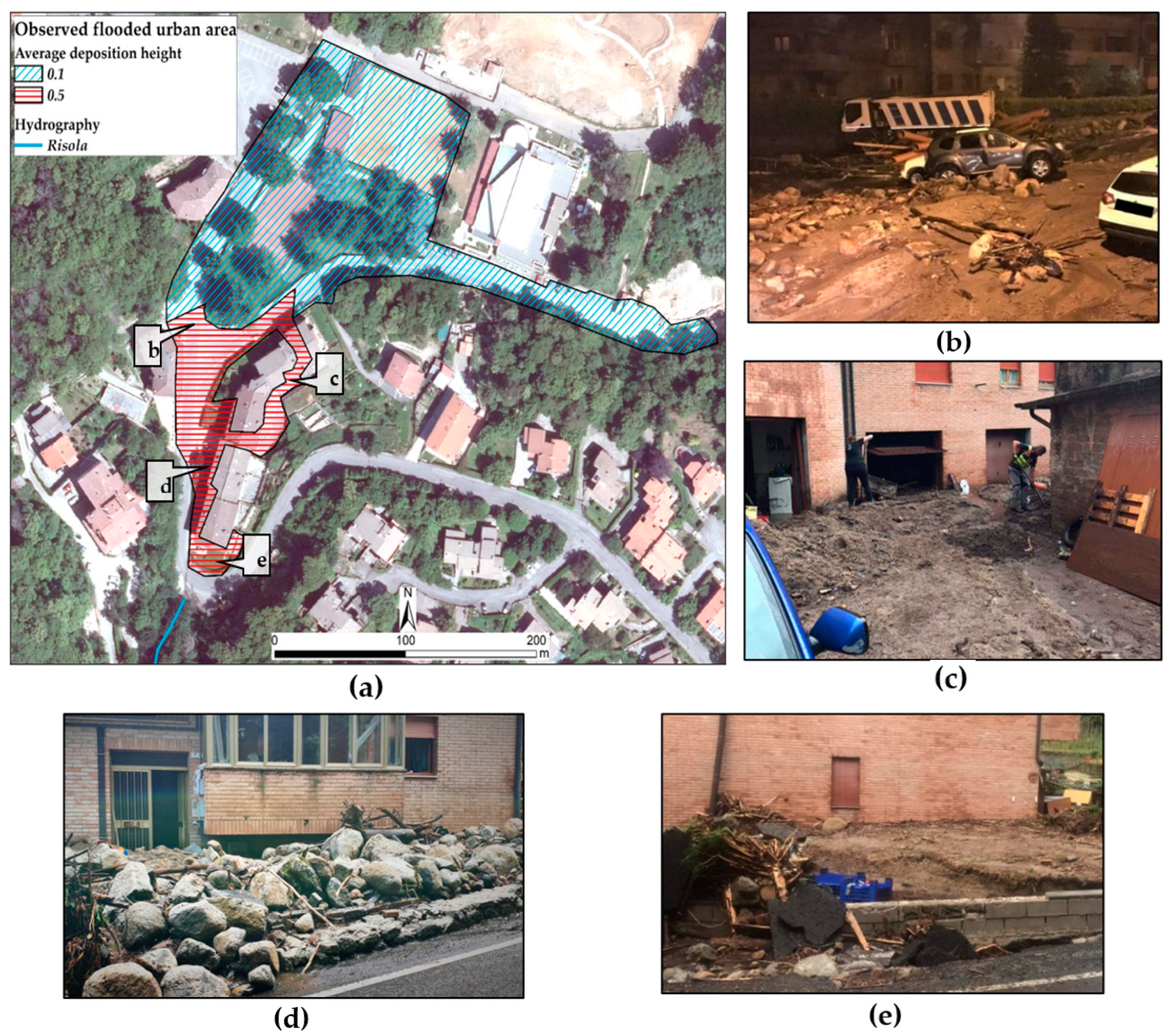
2.1. The 27–28 July 2019 Event

On the night between 27–28 July 2019, an intense meteorological event affected the entire territory of the Tuscany Region. In the Mt. Amiata area, starting at 22:00 on 27 July, the AS rain gauge (Figure 1) recorded rainfall of 210 mm/4 h, with maximum intensity peaks of 45 mm/15 min, never recorded before during the summer months [40].
The processing of the available data for rainfall in the Mt. Amiata area [28] with a 15′-time scan shows that the highest intensity occurred between 22:45 and 23:15 h (Figure 4). In this short period, the rain gauges AS, LV and VA recorded 123, 86, 85 mm of cumulative rainfall, respectively.
The estimated return periods associated with the maximum values recorded in the different durations (1–3–6–12–24 h) are well beyond 200 years [40]. The maximum rainfall values over 12 and 24 h are greater than the recorded historical maximum by more than 60%, which are, to all intents and purposes, absolute outliers, reflecting an extreme weather phenomenon, at least for the available documentation.
The very heavy rain caused widespread flooding in the urban area of Abbadia San Salvatore, but the situation of greatest damage occurred in the area of Via Fosso Canali (Figure 5b–e), where areas of both erosion (the asphalt was eroded) and accumulation of coarse debris, mixed with wood, developed.
From the analysis of the post-event photos, an average deposit thickness of 0.3 m may be estimated in the buried portion of the urban area (Figure 5a), resulting in approximately 2000 m3 of debris, which was removed in a few hours after the event. For this reason, it was not possible to proceed with a field survey to delimit their aerial extension. However, post-event photos and testimonies collected from residents were considered for the evaluation of the flooded area. Analyzing some post-event photos showing the deposit (Figure 5b–e), it was possible to identify two deposition zones differing in thickness of deposited material, as well as their granulometric class (Figure 5a): (i) an area characterized by the deposition of both coarse and finer material with an average thickness of 0.5 m (red polygon); (ii) an area characterized by the deposition of predominantly sandy material with an average thickness of 0.1 m (blue polygon).
The flooding of the urban area has been due to the occlusion of the Risola culvert (dimensions 1.40 m wide × 1.00 m high), caused by a clogging phenomenon of the transported material (mainly debris with some wood). From the testimonies collected among the inhabitants of the area (video [41] and interviews), the clogging of the Risola culvert occurred between 23:30 and 23:45, i.e., almost coeval with the most intense phase of the rainfall. The event affected houses, commercial activities, and cars, causing EUR millions of damages [42].
Further quantitative information about the event, useful for back-analysis of the phenomena, was obtained from the scars caused by the impacts of solid material on the barks of some trees near the creek bed upstream of the culvert. They indicate that the maximum level of the flow above the actual stream bed was approximately 0.5 m, but in particularly narrow sections measuring (<5 m) 1.5 m were reached. The visual analysis of the material deposited in the urban area, as well as the debris present in the riverbed after the event, allowed us to identify the type of phenomenon that occurred: the prevalence of sandy-gravel material, the occurrence of metric-sized boulders and the negligible amount of fine cohesive material suggest that the phenomenon was essentially a flow of water with loose granular material.
Finally, the presence of a flat river stretch upstream of the red star in Figure 1, and the indication that the clogging of the culvert occurred essentially in conjunction with the rainfall peak, suggest that the phenomenon can be categorized among the debris flows with hydrological forcing.

3. Methodologies

This section describes the modelling chain, the specific models chosen for each chain steps and the approach developed for the simulation of culvert clogging that will be used in the back-analysis of the 27–28 July 2019 event. Nevertheless, the geological and geomorphological analysis, already described in Section 2 for convenience, must be considered as the first step of the whole methodology.
As described in Section 2.1, the event can be classified among the debris flows with hydrological forcing. In this case, the formation of the debris flow can be schematized as in Figure 6 (dashed rectangles): surface runoff forms in the upper part of the basin where sediment transport is negligible; then, a stretch of debris flow formation follows downstream, characterized by a flow of water and sediments deriving prevalently from a bed erosion; this is followed by a final stretch, where some further erosion may occur, but the main process is the deposition of the material transported by the flow [43].
In many cases, as in the present one, the detailed studies focus only on the area around the location of settlements subject to possible hazards, and usually this area corresponds to the deposition zone (rightmost dashed rectangle, Figure 6). In such conditions, it is possible to use an approach based on a cascade of models (filled rectangles, Figure 6): a hydrological model, closed in a suitable section close to the beginning of the study area, can be used to estimate a liquid hydrograph (Section 3.1); the debris flow formation transept is not described with a model, but we limit to evaluate the solid and mixture discharges as a function of time in the input section of the debris-flow model by using a suitable “amplification factor” (Section 3.2); finally, the simulation of the mixture flow in the last part of the basin can be obtained with a debris-flow model (Section 3.3). However, the Risola debris flow presents the clogging of a closed section (culvert), a phenomenon that debris flow models do not commonly consider. Therefore, we had to develop a specific procedure to face this aspect; a procedure which is presented in Section 3.4.
The input dataset used for the hydrological modelling was implemented employing the ArcGIS 10.7™ software (ESRI, Redlands, CA), while the one used for the debris flow modelling was implemented with both ArcGIS 10.7™ and the WEEZARD system [44].

3.1. Hydrological Modelling: The FLO-2D Model

Following the conceptual scheme of Figure 6, the first step to be considered is the hydrological modelling of the event. As the Risola is an ungauged catchment, a physically-based rainfall-runoff model was necessary to determine the liquid hydrograph in the required section. For this purpose, we used the FLO-2D model [12,13], a hydrologic-hydraulic model that simulates the overland flow (over slopes and in channelized reaches) fed by the rain (source term) and drained by infiltration (sink term). FLO-2D is a well-established model and it is widely used for hydraulic modelling of debris flows, as well as for hydrological modelling, as in this study, e.g. [45,46,47,48].
The underlying mathematical approach to flow propagation is based on the dynamic wave approximation of the mass and momentum equations. The relevant differential equations are integrated over a regular Cartesian grid defining the topography of the computational domain.
FLO-2D model has three possible different approaches to describe the infiltration [13]. The formulation used in this study case is the Green-Ampt (G-A) equation [49], a physically-based equation based on the soil porous media characteristics [50], which is widely used in hydrologic studies as it has a relatively low computational demand while providing reasonably accurate physical mechanisms [51,52,53,54]. When the maximum infiltration capacity is exceeded, surface flow is generated. Moreover, FLO-2D has the capability of simulating the presence of impermeable layers by assuming a limit to the infiltration depth.
In the following section, we describe the physical quantities (parameters) required by FLO-2D to set up a hydrological simulation with the G-A approach.

Data Input of the Hydrological Modelling

The following parameters are required independently of the infiltration method used.
  • D E M : to obtain the domain for the case study, two Digital Elevation Models (DEMs) were merged, one based on LiDAR acquisition with a cell size of 1 m, and one with a cell size of 10 m, since the first one did not cover the Mt. Amiata summit area [55].
  • n : the Manning roughness [s/m1/3] was spatially assigned reclassifying the land use map [56], according to the value proposed by [57,58].
  • T O L : this parameter expresses the minimum flow depth [m] before runoff volume is exchanged with adjacent grid elements and represents the volume of water stored in small depressions (puddles) that do not become part of the overland runoff or infiltration.
  • Rain: rainfall simulation was obtained by spatializing the rainfall data (mm/15’) from the three available rain gauges (Figure 1) using the Inverse Distance Weight (IDW) method [59].
The G-A equation, based on Darcy’s law, is:
Δ F γ l n ( 1 + Δ F γ + F ( t ) ) = K γ Δ t
where Δ t is the computational time step, Δ F is the change in infiltration (mm) over the computational time step, F ( t )   is total infiltration at time t . The parameters of these equations are: K   is the saturated hydraulic conductivity (mm/h) and finally γ = ( P S I F + H e a d ) · D T H E T A where P S I F is capillary suction (mm), H e a d is the incremental rainfall for the time step plus flow depth on the grid element (mm) and D T H E T A is volumetric soil moisture deficit (dimensionless) function of the effective porosity of the soil.
Finally, the following spatially distributed parameters, affecting the runoff calculation, must be assigned.
  • Impervious areas (%): the portion of a grid element that is impervious to infiltration (e.g., rock outcrops or urban areas).
  • Initial abstraction (mm): the initial loss of rainfall that precedes infiltration and excess rainfall-runoff (e.g., vegetation interception).

3.2. The Debris-Flow Mixture Hydrograph

The mixture hydrograph to be used as boundary condition in the inflow section of the debris flow model, is calculated based on the liquid hydrograph obtained with the hydrological model. The relation, proposed by [2], is the following:
Q m i x   ( t ) = c b c b c ˜ Q h y d r o l   ( t )
where Q m i x   ( t ) is the mixture discharge, Q h y d r o l   ( t ) is the liquid discharge and c ˜ is a reference concentration, which can be estimated through the following relation:
c ˜ = min [ 1 Δ i f tan ϕ d i f ,   0.9 c b ]
where i f   is the average bed slope near the inflow section, Δ = ( ρ s ρ w ) / ρ w is the relative reduced density of the solid material, and ϕ d is the dynamic friction angle of the material.

3.3. Debris Flow Modelling: The TRENT2D Model

Since the solid part of the debris flow we are interested in is characterized by a loose coarse material (see the end of Section 2.1) and the flow occurs both on a fixed and mobile bed, the model we have chosen is the TRENT2D model.
TRENT2D (an acronym for Transport in Rapidly Evolving, Natural Torrent), represents one of the most advanced two-dimensional models for the study of granular debris flows and intense solid transport phenomena. In this Section we describe the main mathematical features of the model, addressing the reader to Appendix A and the original paper for more specific mathematical aspects. In addition, in Section 3.3.1, we highlight the characteristics of the WEEZARD system used for the management of the input data, launching the simulations, and for the results analysis.
The TRENT2D uses a two-phase isokinetic description of the mixture that composes the flow, where the solid and liquid components are considered and described, from the point of view of the equations of motion, in a separate but interacting way. A second characterizing element concerns the description of the bed, over which the debris flow flows. In the original formulation of the TRENT2D, the movement of the mixture occurs on a mobile bed, i.e., on a bed that can be subject to erosion and deposition during the motion. However, a more recent version of the model [60] also allows the consideration of cases where the mixture flows on a non-erodible bed. In the latter case, the model provides for the possibility of depositing material above the non-erodible bed (thus becoming, at least temporarily erodible), but prevents the bed from reaching, due to erosion, elevation below the level of the non-erodible layer. A third aspect, intimately related to the description of the bed, concerns the composition of the mixture: as it is a two-phase model, the average volumetric concentration of sediment on the vertical is variable in space and time and is related to the local hydrodynamic conditions. The formulation used is as follows:
c = c b β | u | 2 g h
where c b is the concentration in the bed (equal to 1 p , where p is the porosity of the material) considered constant, β is a transport parameter to be determined based on the flow and sediment characteristics, u is the depth-averaged velocity vector of the mixture, g is the acceleration of gravity and, finally, h is the flow depth (difference in elevation between the free surface of the flow and the bed). The variability in concentration is related to the exchange of sediment and water that occurs between the bed and the flow during erosion and deposition phenomena. It is worth noting that with a two-phase approach, the mixture cannot stop as a whole, but only the solid phase (and the liquid part necessary for the saturation of the material) stops, while the liquid phase flows away. A fourth aspect concerns the formulation of the global law of resistance to motion. It is given by the resistance of the liquid phase plus the resistance of the solid phase, which, in the flows, is predominant and is mainly related to collisional phenomena. The law used in the TRENT2D model is that proposed by [61] and considers only the collisional contribution:
τ 0 ρ w = [ 25 4 a ( Δ + 1 ) sin ϕ d λ 2 Y 2 | u | ] u
where τ 0 is the bed shear stress, ρ w is the water density, a = 0.32 according to [61], Δ = ( ρ s ρ w ) / ρ w is the relative reduced density of the solid material, ϕ d is the dynamic friction angle of the material, λ = [ ( c b / c ) 1 / 3 1 ] 1 is the linear concentration, Y = ( h / d ) is the submergence, where d is a characteristic diameter of the transported material and h is the local mixture depth.
In the case of a fixed bed, concentration is no longer connected to the local flow conditions (namely, Equation (4) does not hold), and it becomes a simple advected quantity. As for the bed shear stress, a classical Strickler relation was used, namely:
τ 0 ρ w = g ( K s ) 2 h 1 / 3 | u | u
where K s is the Strickler’s coefficient.

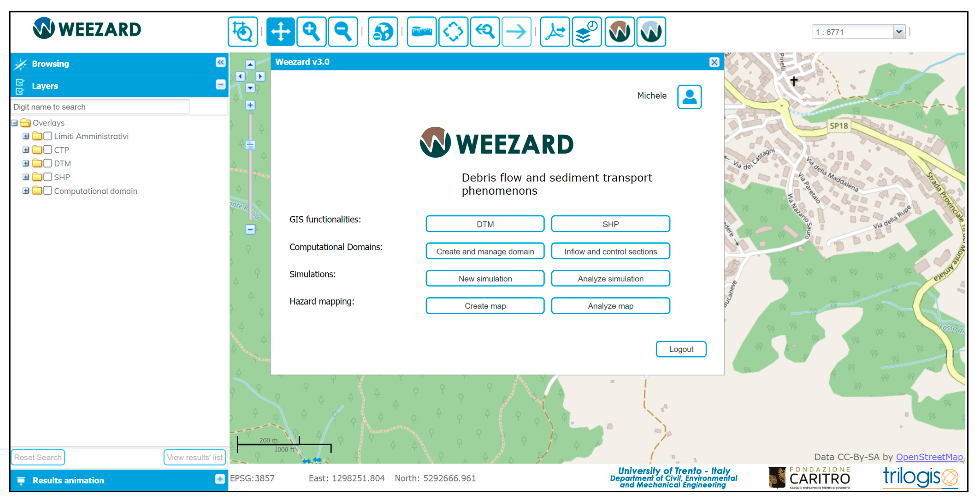
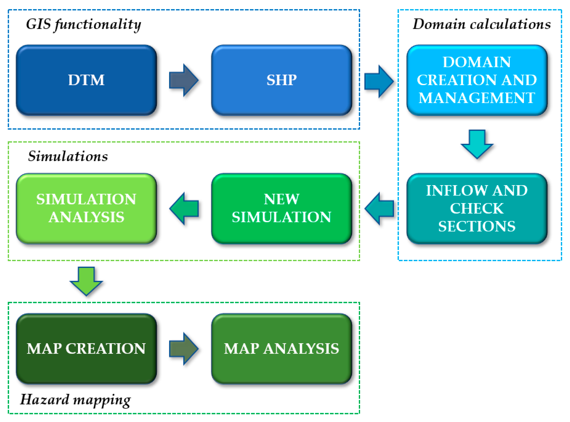
3.3.1. The WEEZARD System

WEEZARD (WEbgis modElling and haZard Assessment for mountain flows: An integRated system in clouD) is a system that allows the management of all phases of data preparation, execution of simulations, analysis of results and production of hazard maps for a range of phenomena that may affect mountain environments (debris flows, intense solid transport phenomena, mudflows, dense snow avalanches). The key difference from a simple management interface that normally operates locally on a computer is that it is based on an innovative web services system [44] accessed through a common network browser [62] (Figure 7).
This approach has several advantages over a local system, first the fact that it is not necessary to have a high-performance computer to be able to do even computationally heavy simulations as a shared network server is used. It is just the sharing of the resource of calculation the key aspect that allows the use of sophisticated instruments of simulation at low cost, as demanded by the European directive [10]. A second element that characterizes this system is its ease of use. Indeed, WEEZARD is a word that recalls another English word, wizard, that in the computer science language indicates a procedure, generally incorporated into a more complex application, that allows the user to carry out determined operations (usually articulated) through a series of simple steps in succession. Having wizards to easily perform a complicated set of operations, such as those required to simulate natural hazards in a mountain environment, is a fundamental prerequisite for transforming an inherently complex system into an effective, efficient, and economical tool for professional use.
In extreme synthesis, the process that, from the acquisition of basic data, leads to the result of the elaboration of a hazard map, can be divided into a series of logical steps (Figure 8), independent of the type of natural hazard one wants to simulate. For each of these steps, a series of functionalities are available that allow us to easily perform a whole series of operations related to that logical step (each functionality is illustrated through video tutorials [63]) and that greatly facilitate the learning and use of the system.

3.4. A Novel Approach for the Simulation of Culvert Clogging

As a result of the presence of large sediments and boulders in the flow (see Section 2), we assumed that clogging occurs once the level of the debris flow reaches the upper level of the culvert. Therefore, we distinguish the following: (i) a pre-clogging phase, lasting from the beginning of the event up to the instant in which the debris flow level, near the culvert inlet, exceeds the value of the culvert coverage level (conventional clogging time); and (ii) a post-clogging phase, characterized by an obstructed section near the culvert inlet, lasting from the conventional clogging time up to the end of the phenomenon. In the following sections we present the strategy and the input data required by the TRENT2D model to implement the two phases.
It is worth noting that, since the a priori exact clogging time is unknown, a complete simulation with the modified computational domain (as specified further on) must be performed and, a posteriori, the conventional clogging time can be identified.

3.4.1. Strategy and Data Input of the Pre-Clogging Phase

In the pre-clogging phase, to describe the motion in the culvert, its closed section must be transformed, in the computational domain, into an open channel with walls up to the ground level in which a free-surface flow can occur.
The parameters used in the pre-clogging phase, and how they were evaluated are described below.
  • Computational domain: the first element to be defined is the computational domain constituted by a square Cartesian grid defining the altimetric base of the study area. Moreover, non-erodible areas and erodible areas with the associated depth of the erodible material can be specified.
  • Inflow conditions: the inflow condition must be imposed in the section where the debris flow is expected to enter the computational domain. By using the WEEZARD system, the mixture hydrograph is evaluated automatically, given Q h y d r o l and the inflow section as described in Section 3.2.
The following parameters can be chosen a priori, since they are closely related to measurable properties, and kept constant in all the simulations.
  • Debris parameters: include the values of the sediment bed concentration c b , the dynamic friction angle ϕ d , and the reduced relative sediment density Δ .
On the other hand, the following parameters can be estimated as follows.
  • Y : can be evaluated by using an average value of the transported grain size and a reference depth along the flow.
  • β : is determined by assuming a local uniform flow condition in the input section with the resistance law according to [61]:
β = c ˜ c b i f λ 2 1 + c ˜ Δ 25 4 a ( Δ + 1 ) sin ϕ d Y 2
where c ˜ is given by Equation (3). β is calculated directly by the WEEZARD system based on the other input parameters.
  • K s : the Gauckler–Strickler roughness coefficient can be assigned based on the land use categories [56], according to [57,58].

3.4.2. Strategy and Data Input of the Post-Clogging Phase

Starting from the conventional clogging time, the mixture stops flowing into the culvert and the entrance section becomes an impermeable wall. To describe this phase, the altimetry of the computational domain must be changed accordingly.
  • Instead of the artificial channel bed, the original ground level must be restored along the culvert path.
  • In the channel upstream of the culvert, from the inlet section to the culvert initial section, the original DEM must be changed according to the bed modifications obtained in the pre-clogging phase. The resulting DEM can be used as the initial condition for this phase.
The values of all the parameters used in the pre-clogging phase can also be maintained in the post-clogging phase.

4. Results

In this section, we present the results of the back-analysis of the Risola debris flow obtained from the application of the methodology described in the previous sections. To allow the reproducibility of the results, for each step of the modelling we also provide the values of the employed parameters and, when available, a comparison of the results with measured/estimated data.

4.1. Hydrological Modelling: Parameter Values and Results

The parameters used for the hydrological modelling are herein described.
  • D E M : the two DEMs with different spatial resolutions were mosaicked and resampled to a common cell size of 5 m, obtaining a good compromise between the representation of the hydrographic network and the computational time necessary to run the simulation.
  • T O L : The minimum value of 0.0012 m was used, as recommended in the FLO-2D manual [13]. Using higher values would result in larger quantities of water that do not become part of the overland runoff or infiltration. A situation that, due to the characteristics of the study area, would not be justified from a hydrological point of view.
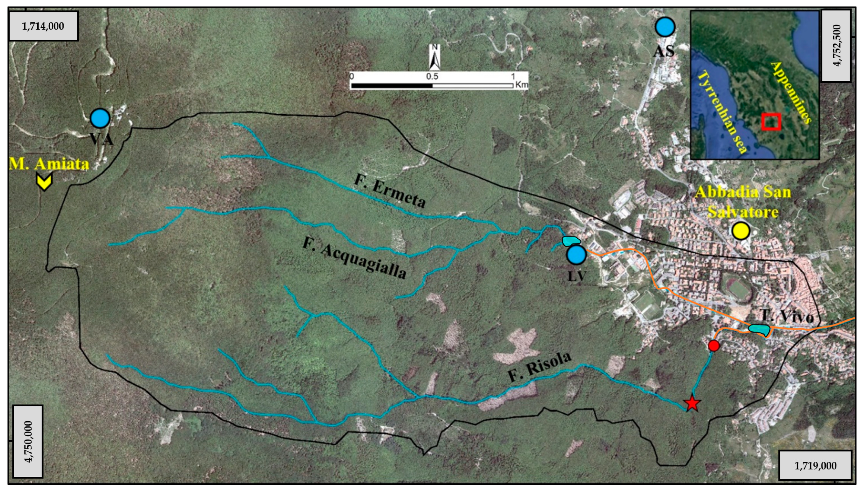
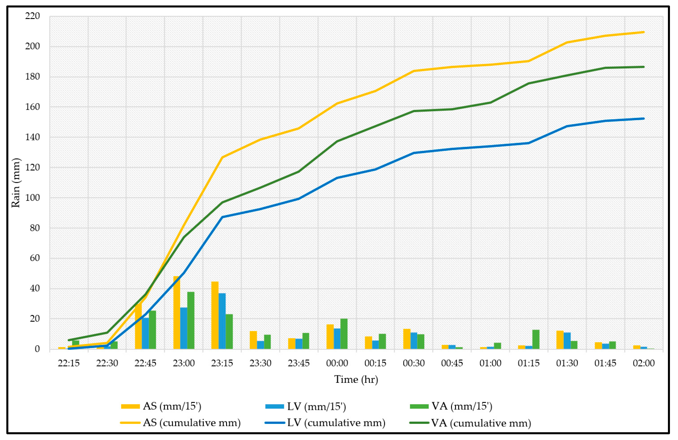
  • Rain: to apply the IDW method for the entire study area considering the data from the AS, LV, and VA rain gauges (Figure 1) only, an auxiliary gauge was placed south of the southern border of the Risola catchment, allowing us to extend the rainfall maps to the Risola catchment area. This was achieved by placing a barrier feature between the auxiliary gauge and the existing rain gauges without altering their rainfall data. A barrier is a polyline dataset used as a breakline that limits the searching region for input sample points: only those points located on the same side of the barrier are considered. Thus, a representation of the rainstorm distributed in time and space was obtained.
  • K 
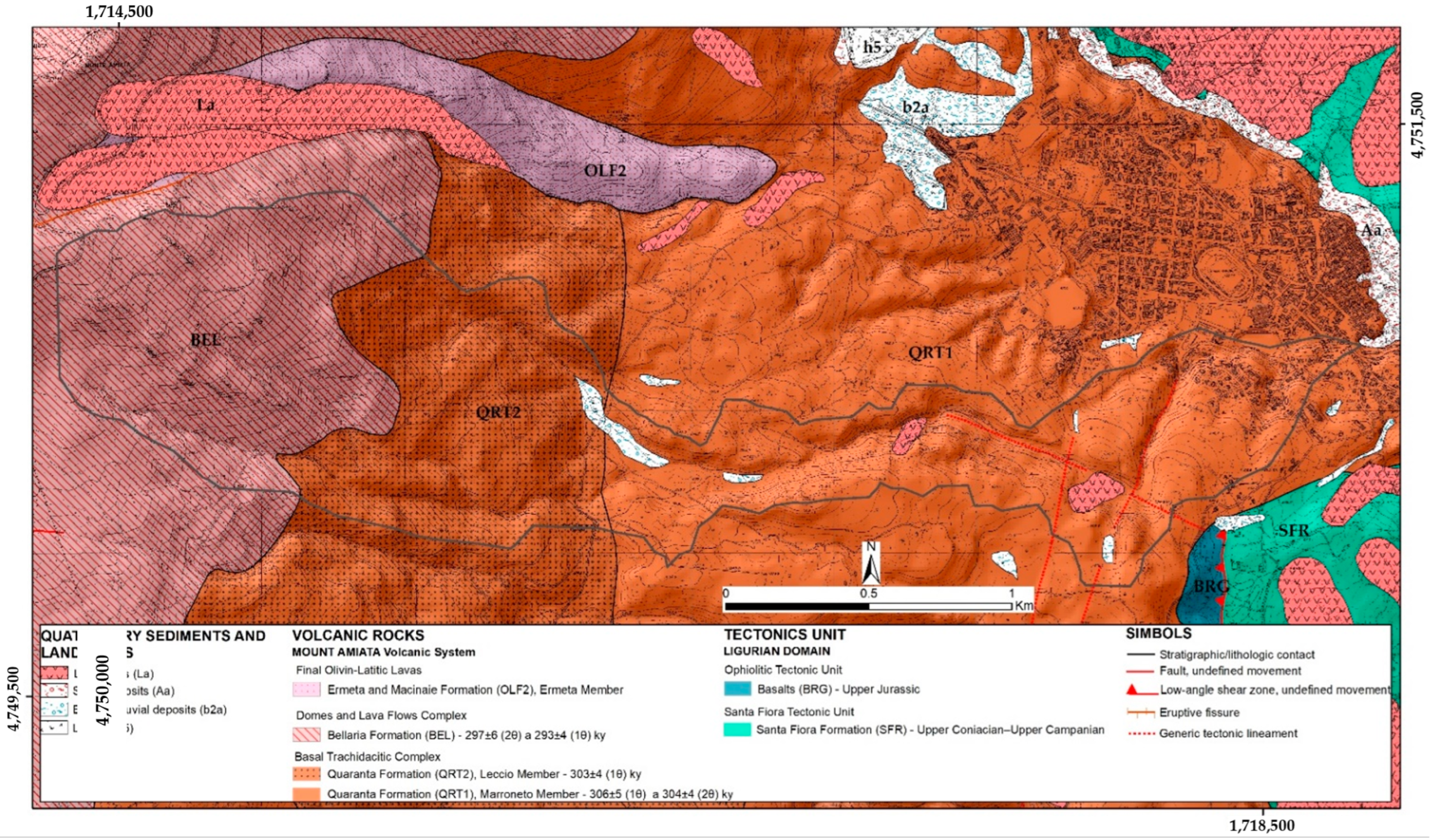
: a specific survey was conducted through constant-head measurements with an Aardvark-type permeameter [64] to determine the value of field saturated hydraulic conductivity. Thirteen borehole tests were performed within the sandy soil above the BEL2 and QRT volcanic formations, investigating depths between 0.30–1.50 m. Given the homogenous nature of the unconsolidated material in the study area, the average value (140 mm/h) was uniformly assigned throughout the catchment.
  • D T H E T A : in the five days preceding the event, the three rain gauges close to the study area (Figure 1) recorded no rainfall accumulation, and considering a longer period (i.e., 60 days), only 28 mm were recorded. This extended drought period and the permeable nature of the unconsolidated material indicate that the antecedent moisture conditions before the event were dry. Thus, the assumed D T H E T A value for modelling is 0.35, as also specified in the FLO-2D manual [13]. Only in the last stretch of the Risola up to the culvert (~1 km) can the soil be considered saturated. In fact, some ephemeral springs with a flow rate of only a few l/s (negligible if compared to the discharge developed during the event) bring water into the stream bed.
  • P S I F : the obtained value of this parameter is equal to 30 mm. This is in agreement with the values proposed by [65].
  • Given the geological characteristics of the study area (Section 2), no impermeable boundary was imposed at the bottom of the unconsolidated material of the catchment.
Finally, the following parameters were spatially assigned by reclassifying the land use map [56] using the described criteria.
  • Impervious areas (%): as described in Section 2, the bedrock of the study area is affected by widespread weathering. For this reason, infiltration is set to zero for the fractured bedrock portion (type (i) in Section 2; ~15% of the total catchment area) even though no data are available on the rock mass fracturing degree and the related infiltration patterns. It may be noted that this assumption is probably reasonable for the study area only in the case of short and intense rainstorms, such as the one analyzed here.
  • Initial abstraction (mm): it represents the initial loss of rainfall that precedes infiltration and excess rainfall-runoff (e.g., vegetation interception). This parameter was assigned using the values proposed in the FLO-2D manual [13].
The input dataset used for the hydrological modelling is summarized in Table 2.
The resulting hydrograph is presented in Figure 9 (green line) and it is referred to where the closure section of the basin coincides with the inflow section of the debris flow model, indicated with a red star in Figure 1.

4.2. The Debris Flow Hydrograph

The mixture discharge (Figure 9) was obtained using Equations (2) and (3) as reported in Section 3.2. The parameter values employed are described below.
  • Debris parameters: the values of c b , ϕ d , and Δ parameters used in this study are those generally accepted in debris flow dynamics [61] and are reported in Table 3. This assumption stems from the fact that the material involved does not have any peculiar geotechnical characteristics that would necessitate changing the values of these three parameters.
  • i f 
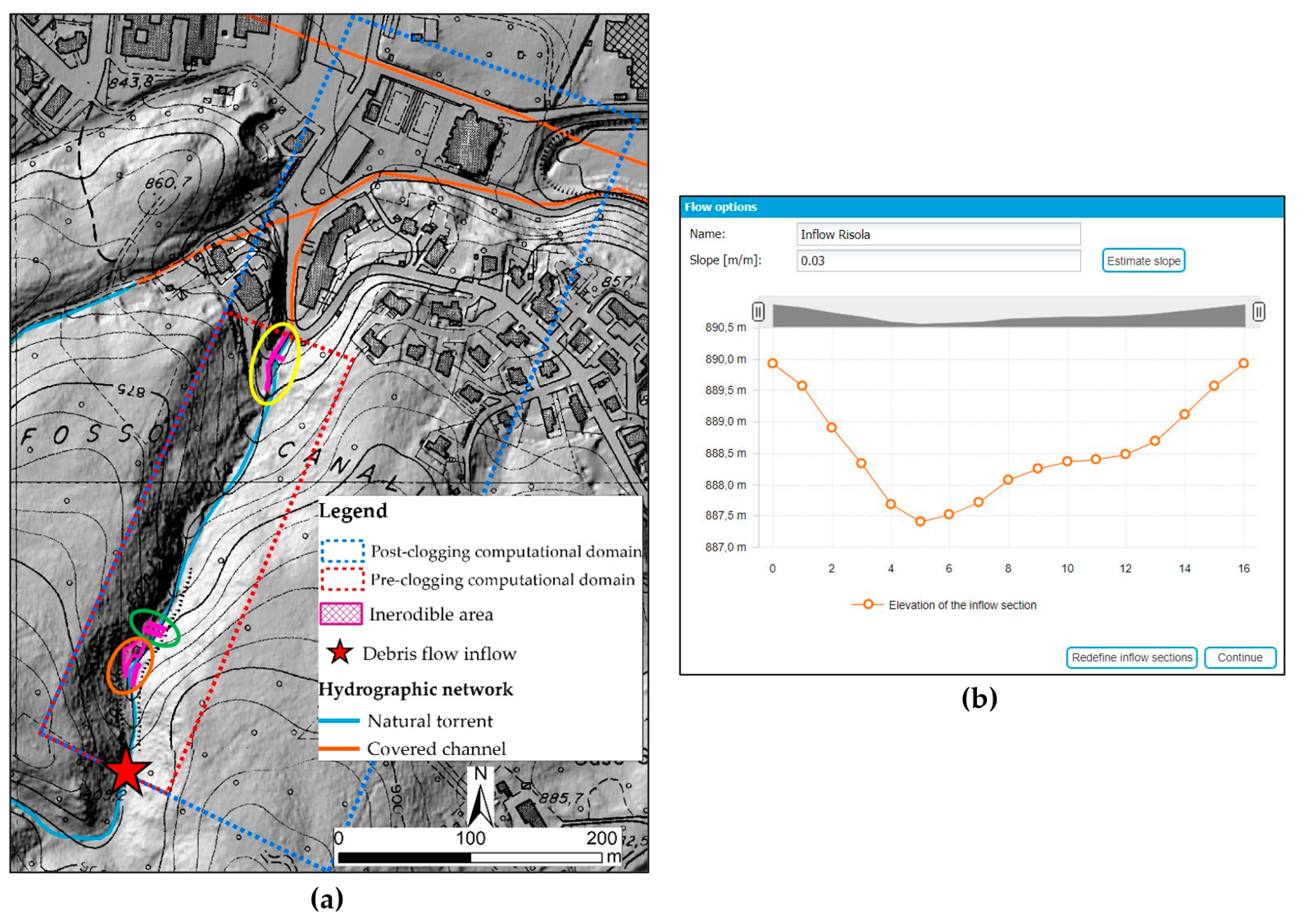
: the slope of the inflow section was set according to the morphological characteristics of the stream, equal to 0.03 m/m, i.e., the average value between the upstream and downstream reaches of the input section, with slopes of about 0.01 m/m and 0.05 m/m, respectively. This choice derives from the geomorphological characteristics of the Risola just upstream of the red star in Figure 1, where an abrupt change in direction and slope of the creek occurs (see Section 2).

4.3. Pre-Clogging Debris Flow Modelling: Parameter Values and Results

The parameters used for the pre-clogging modelling are reported in the following list with a description of the reason for their choice.
  • Computational domain: an available DEM [55] with a cell size of 1 m × 1 m, based on LiDAR acquisition, was used to produce the domain, which is delimited with a red dashed rectangle in Figure 10a. The resulting morphology of the inflow section (Figure 10b) is referred to as the red star in Figure 10a. To represent the culvert width with a reasonable approximation and considering that its width is 1.4 m, the original DEM was resampled to a cell size of 0.5 m × 0.5 m. In this way, the channel is represented by using three cells, namely with a width of 1.5 m, and the deviation of 0.1 m was assumed to be negligible for the modelling results. In addition, as the base of the culvert is located 1.5 m below the road level, the resampled DEM was lowered by 1.5 m along the path of the culvert. In the analyzed stretch, some anthropogenic structures are present, thus erodible, and non-erodible zones have been defined accordingly. One of these structures is a small building preceded by a short (~25 m) non-erodible artificial portion of the bottom of the creek, and a wall on the right bank of the stream (orange circle in Figure 10a). In addition, three check dams are located along the Risola: two of them are placed immediately downstream of the building described previously (see the green circle in Figure 10a), and the last check dam is located just upstream of the culvert inlet section. In this last area, two walls bound the creek before the entrance to the covered portion (yellow circle in Figure 10a). These structures, which are correctly represented by the DEM used for the modelling, are treated as non-erodible areas with null erodible thickness. On the other hand, the rest of the torrent is treated as an erodible area.
  • Y : to choose the optimal value for this parameter, we performed tests with values of 15, 10 and five. Results show that for values of 15 and 10 the flow depths are too shallow compared to those observed. At the same time, the erosions were excessive, generating a higher concentrated flow and, consequently, culvert clogging time earlier than observed. On the other hand, for Y = 5 , both the flow depths along the stream and the culvert clogging time were found to be consistent with the observations.
  • β :   the value of the transport parameter used for the numerical modelling was obtained considering the submergence as Y = 5 , and considering the values of other parameters appearing in Equation (7) as reported in Table 3.
Figure 10. (a) The lower portion of the Risola where the dashed red border corresponds to the computational domain of the pre-clogging simulation, while the blue box is related to the domain of the post-clogging modelling; (b) the morphology of the inflow section at the red star.
Geosciences 12 00385 g010
In this phase of the back-analysis, the physical quantities we used to validate the numerical results was the clogging time, which occurred between 23:30 and 23:45, as described in Section 2.1. The results of the pre-clogging simulation, performed with the parameters in Table 3, show that the clogging time occurs at about 23:30 (i.e., ~3200 s in Figure 9), as depicted in Figure 11, thus in good agreement with what happened.
Figure 11. Longitudinal profile of the Risola near the entrance of the culvert at the clogging time (~23:30): riverbed level (red line) and free surface level (blue line); in green, the riverbed level at the beginning of the simulation.
Geosciences 12 00385 g011

4.4. Debris Flow Back-Analysis: Post-Clogging Phase Results

The parameters used for this phase are the same as the pre-clogging scenario. The quantities used during this phase to validate the results were the distribution of eroded and deposited material along the Risola, and in the built-up area, as well as the maximum free surface levels reached by the flow.
In Figure 12a, the map of the morphological modification obtained using the post-clogging modelling is compared with the map of the debris flow deposition area obtained by interpreting the archive photos of the event (Figure 5). Overall, there is a good agreement between the observed and modelled debris flow deposition area. The modelled values of the deposit height in the built-up area result to be, on average, equal to about 0.1–0.5 m, while in some points they reach 1 m, in good agreement with the post-event photos (Figure 5b–e). The more accurate modelling results, in terms of both the flooded area and maximum deposit heights, are related to the area marked in red (Figure 12a), where coarse material with an average thickness of 0.5 m was deposited (Figure 5b–e). On the other hand, in some of the areas characterized by thin deposit thicknesses and predominantly fine material, delimited in blue (Figure 12a), the modelling results are less accurate. A comparison with the real flooded area was not possible due to limited data being available (see Section 2.1). However, the comparison between the numerical flooded area (i.e., the area where the mixture has flowed) and the estimated deposition area shows a good agreement (Figure 12b). In particular, it can be noticed that the area of the fine sediment deposition (in blue) was affected by the debris flow phenomena.
The areas where the asphalt cover was damaged were considered as erodible zones for the modelling. Simulation results indicate widespread erosion in these areas, in agreement with field observations. On the other hand, regarding the erosions that occurred along the creek shaft, no direct comparisons were possible with what actually happened during the event. However, the values obtained (maximum values of about 2 m and an average of 0.35 m) are consistent with the known evidence.
The results obtained indicate that the debris flow generated in the Risola eroded and mobilized a debris volume of 3000 m3, of which approximately 1500 m3 partially buried the built-up areas, in line with the estimated value (Section 2.1). Part of this material reached the “Lago Muraglione” reservoir, contributing to its overflow, which in turn caused the flooding of its downstream area.
Finally, since the obtained results were considered satisfactory in terms of the timing of clogging, maximum heights reached by the flow, flooding extension and the volumes deposited, no further sensitivity analyses were performed.

5. Discussion

In this paper, we have presented: (i) a multidisciplinary approach for the study of a debris flow, in which the clogging of a culvert plays a fundamental role in the dynamics of the occurrence; and (ii) the application of this methodology to a back-analysis of a case study. Results show that the event can be reproduced reasonably well, thus allowing the validation of the approach. In the following sections, we analyze critically what we think are the main issues of the used methodology in relation to the obtained results.

5.1. Geological and Geomorphological Analysis

The Mt. Amiata, where our case study is located, does not present geological and geomorphological features that are characteristic of the Alpine regions [66], namely with the widespread presence of Quaternary deposits of moraine and/or fluvioglacial origin that makes these areas prone to debris flows. Considering exclusively the existing cartographic data (Figure 2), the area presents a low susceptibility to these kinds of natural hazards due to the apparent lack of source sediments. In the Risola catchment, there are only small areas of eluvial–colluvial deposits, and two landslides, apparently connected to the hydrographic network. Despite this situation, the 2019 occurrence demonstrated that a source of debris had to be present. A field survey revealed the widespread availability in the Risola catchment of loose solid material caused by saprolitic weathering of the volcanic bedrock, both in the hydrographic network and on the slopes, as explained in detail in Section 2. Surveys aimed at the geological and geomorphological characterization of an area are therefore fundamental prerequisites for a back analysis but are equally important in predictive hazard mapping activities and in planning of hydrogeological risk reduction [67]. This is also emphasized by the ongoing climate change characterized by more frequent extreme rainstorms causing mass movement in areas usually not affected by such events.

5.2. The Choice of the Models

As highlighted by other studies, e.g., [68,69,70], the use of a cascade of models is an effective way to simulate the connection between rainfall, hydrological processes, transport of sediments and bed modifications in several debris flow phenomena characterized by a clear hydrologic forcing (the so-called runoff-generated debris flows, e.g., [71]). However, the choice of advanced, physically based models as cascade elements is somewhat compulsory when: (i) the available data does not allow a detailed calibration; (ii) we want to make predictive analyses. Since in this work the former applied, we choose to use the models described in Section 3 as both models use physically based parameters that can be determined a priori or with minor calibration.
As for the hydrological model, the FLO-2D with the Green-Ampt description of the infiltration appeared to be a suitable choice that utilized the knowledge of the basin derived from the field survey.
As for the debris flow model, the TRENT2D, based on a two-phase, mobile-bed approach, appeared to be the most appropriate in comparison with other commercial codes employing a single-phase approach, which is unable to catch some of the most important processes observed in the analyzed event, namely a granular debris flow. For example, the FLO-2D debris flow model uses a fixed-bed description that is unable to describe both erosions and depositions occurring during the flow, but the variation in the bed elevation can occur only when the single-phase fluid stops (final deposition), occurring when the bed shear stress is lower than a threshold (Bingham fluid [13]). The RAMMS model uses an entrainment function that changes the flowing volume, but in the calculations, the bed is kept fixed [72]. In any case, in single-phase models the mass eroded or deposited has a composition (represented by the solid volumetric concentration) that is different with respect to the flowing mass: the solid concentration of the flowing mass is always lower than the bed concentration [2,73]. For this reason, while a two-phase model is able to deal with the change in the concentration of the flowing mass and with the consequence of this change (for example, the bed shear stress is a function of the concentration), the single-phase models with constant density simply cannot.
Results of the back-analysis confirm that the choice of the models we have performed was reasonable and that this choice should ensure adequate accuracy in predictive situations.

5.3. The Culvert Clogging and Its Numerical Simulation

Although the clogging of a culvert (or other hydraulic structures) by debris flow is a widespread phenomenon affecting many mountainous urban areas, few case studies focused on its numerical modelling systematically. Moreover, the most popular and widely used hydraulic models, such as FLO-2D [13] or HEC-RAS [74], allow the clogging of hydraulic structures (e.g., bridges, culverts, and storm drain systems) but only by establishing a priori both the percentage and the time of blockage (see e.g., [75]). TELEMAC-2D software [76] also allows hydraulic modelling considering the presence of culverts, however, this model is used for the simulation of water floods in a fluvial environment (see, e.g., [77]) and is not able to simulate a blockage caused by debris flows or intense solid transport phenomena. In addition, these models are single-phase and fixed-bed models.
At the current state of the art, neither two-phase, mobile-bed models can manage directly the debris flow clogging of a closed section. Therefore, our choice to define a practical methodology was compulsory.
Indeed, we do not know when the clogging actually happens, the possible dependence on the grain size and the culvert area, and if a pressurized flow occurs before the clogging. A thorough experimental study is therefore necessary to shed light on this issue but, in the meantime, a reasonable practical approach is desirable.
Despite the simplicity of our assumptions (Section 3.4), results are consistent with reality, in terms of the timing of clogging as highlighted in the pre-clogging phase results (Section 4.3), as well as in terms of non-excessive erosion and deposition processes obtained at the end of the post-clogging simulation (Section 4.4).
We are aware that the successful application of the novel procedure in a specific case does not allow us to assert that it will work in any case. Pending further possible confirmation of the already planned experimental study, we are confident that this novel approach can be applied in hazard mapping activities.

5.4. Comparison of Simulated and Observed Data

Comparison of simulated and field data is never easy in the case of debris flows. One of the main issues is the lack of accurate post-event filed measurement. The reason is that these events are linked to dangerous situations, damage and even fatalities and therefore, since measurements are not a priority in these circumstances, they are often not promptly performed in undisturbed conditions. Moreover, many times measurements are not direct, and many others are only estimates, whose uncertainty cannot be determined.
As explained in Section 2.1, the mapping of the flooded area is subject to some inevitable uncertainty. The planimetric accuracy is therefore limited and any point comparison with simulated data has no meaning in the present case. In any case, it is possible to notice that in some areas the comparison is better while in others the difference is more significant. In particular, in the area with deposition of coarse debris and an average thickness of 0.5 m (delimited in red in Figure 12a), the results obtained with the modelling are consistent with what was observed, both in terms of thickness and flooded area. On the other hand, in the area of fine sediment deposition with an average thickness of 0.1 m (marked in blue), the results of the deposition height are less accurate, with calculated deposits lower than the estimated ones. It is worth noting that in the red area, the dimension of the sediments was significant, while the blue area was characterized by very fine sediments. This difference justifies the different performance of the used debris flow model: since the composition of the transported material is assumed to be constant, the model has been tuned to simulate the coarse material characterizing the bed in the upper part of the computational domain. Therefore, it cannot be so accurate in describing zones with very fine material.
Last but not least, in the present study, we have also used the temporal datum to make the comparison. This is a very lucky situation since such data is not commonly available.

6. Conclusions

After this study, thanks to the results obtained by modelling the debris flow event that occurred in the Risola catchment on 27–28 July 2019, it is possible to state that:
  • A geological-geomorphological model based on the integration of detailed mapping and specific engineering geological field investigations is a fundamental prerequisite for further accurate numerical debris flow modelling.
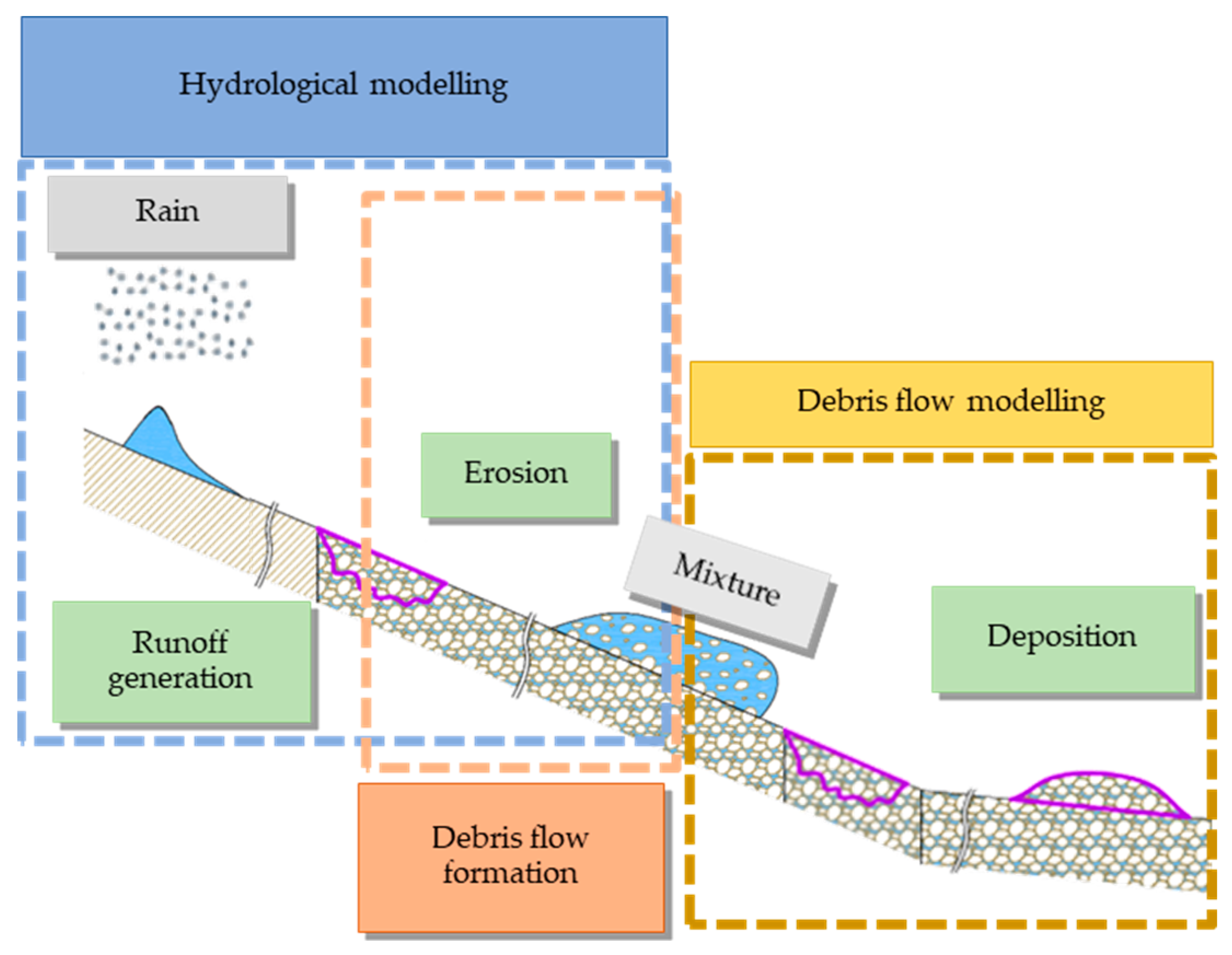
  • The overall methodological approach used in this study, namely a cascade of models composed of a hydrological model for the estimation of the hydraulic forcing, estimation of the mixture flow rate with the amplification factor, and two-phase modelling of the debris flow in the final reach, provides reasonable outputs for the simulation of debris flows with hydrological forcing.
  • The modelling assumptions introduced to overcome some of the limitations of the model used, namely the definition of the conventional occlusion time and the subdivision of the simulation into pre- and post-clogging, proved to be effective.
  • The two-phase approach for debris flow present in the TRENT2D model allows an effective and straightforward description of all the phenomena involving granular debris flows in challenging situations.
  • The WEEZARD system allowed us to handle complex and sophisticated simulations simply, achieving a methodology in line with the European Floods Directive.
  • An additional important result should be emphasized. As the back-analysis was implemented mostly using a priori fixed parameters (as they are physically based) and the parameters determined by calibration (Y and consequently β) are very close to values that can be reasonably a priori estimated, the modelling approach implemented also has a good predictive capability. Indeed, as the observed local mixture depth values range along the stream between 0.30 m and 1.50 m, and assuming an average diameter of the transported material of 0.20 m, the Y parameter can reasonably be in the range 1.5–7.5. This results in an average value of 4.5, which very close to the value of five used in the modelling.
Therefore, we are confident that the implemented modelling approach may be reasonably employed for predictive analysis, such as for hazard mapping and hydraulic design, as well as verification of mitigation structures, and that it may be considered in accordance with the EU Flood Directive as an “appropriate practice and the best available technology that does not imply excessive costs”.

Author Contributions

Conceptualization, G.R., M.A., D.Z. and L.D.; methodology, G.R., M.A., D.Z. and L.D.; software, D.Z., M.A. and G.R.; validation, G.R., L.D., D.Z. and M.A.; formal analysis, G.R., L.D., D.Z. and M.A.; investigation, M.A. and L.M.; resources, G.R. and L.D.; data curation, M.A., G.R. and D.Z.; writing—original draft preparation, M.A. and G.R.; writing—review and editing, M.A., G.R., L.D., D.Z. and L.M.; visualization, equal contribution of all authors; supervision, G.R. and L.D.; project administration, G.R. and L.D.; funding acquisition, G.R. and L.D. All authors have read and agreed to the published version of the manuscript.

Funding

This research was partially funded by CARITRO Foundation—Cassa di Risparmio di Trento e Rovereto within the project “Progetto WEEZARD: un sistema integrato di modellazione matematica a servizio della sicurezza nei confronti di pericoli idrogeologici in ambiente montano”; and it was also funded by Dipartimento di Scienze Fisiche, della Terra e dell’Ambiente within the project “Accordo di collaborazione scientifica tra Unione Comuni Amiata-Val d’Orcia e Università di Siena” (Project leader: L.D.), under grant agreement n. 6100.

Data Availability Statement

All data generated or analysed for this study are included in this article, and the related datasets are available from the corresponding author upon reasonable request.

Acknowledgments

The author is grateful to Pier Lorenzo Fantozzi for his support in this project. The authors wish to thank Daniele Rappuoli and Andrea Esposito of the Unione dei Comuni Amiata-Val d’Orcia Technical Office for providing the post-event photos, and Alberto Bertocci for the information on the culvert dimensions.

Conflicts of Interest

The authors declare no conflict of interest.

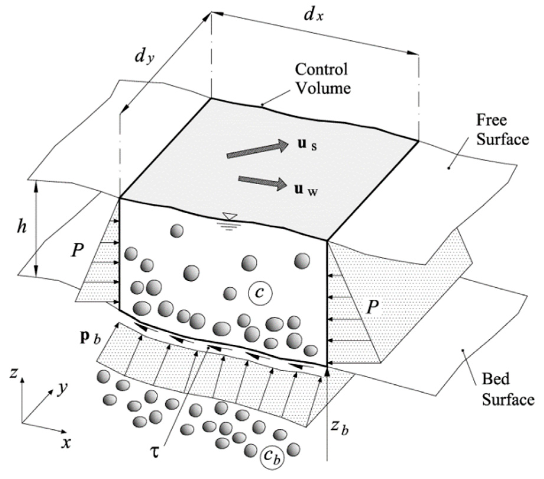
Appendix A. Differential Equations of the Two-Dimensional TRENT2D Model

The differential equations that constitute the TRENT2D model are derived from the principles of conservation of mass and momentum of the components of the mixture. It should be noted that to obtain differential equations one must assume a continuous medium (in practice, a continuous medium occupies all the space of interest) while in a solid–liquid mixture this condition does not occur for the individual phases (each phase occupies the space discretely). To have a continuous approach, the physical quantities used to describe the motion must be properly averaged (e.g., over a reference volume). Therefore, the differential equations that define the model do not describe what happens at a point in space but rather what happens “on average” at that point.
The other assumptions that are considered to derive the system of equations are:
  • the motion of the debris flow occurs predominantly along a flat or weakly curved surface, so the motion is negligible in the direction orthogonal to that surface (a direction assimilated to the vertical), it is well represented through average quantities over the depth, and the pressure distribution is linear.
  • the solid phase is characterized by a representative sediment diameter and constant density.
  • the concentration in the bed is constant.
  • the velocity of the two phases is the same (isokinetic assumption).
Referring to Figure A1, where the reference system, the variables used, and the infinitesimal control volume (in the plane) used for the derivation of the equations are reported, the system of differential equations of the TRENT2D model, considering the assumptions listed above, turns out to be the following:
{ t ( h + z b ) + x u x h + y u y h = 0 t ( c h + c b z b ) + x c u x h + y c u y h = 0 t [ ( 1 + c Δ ) u x h ] + x [ ( 1 + c Δ ) ( u x 2 h + g h 2 2 ) ] + y [ ( 1 + c Δ ) u x u y h ] + ( 1 + c Δ ) g h x z b = τ 0 , x ρ w t [ ( 1 + c Δ ) u y h ] + x [ ( 1 + c Δ ) u x u y h ] + y [ ( 1 + c Δ ) ( u y 2 h + g h 2 2 ) ] + ( 1 + c Δ ) g h y z b = τ 0 , y ρ w
The first two equations express the conservation of the mass of the mixture (sum of the mass conservation equation of both phases) and the solid mass, respectively. Note that the densities of the phases are simplified in the equations as constants. The second two equations express the conservation of momentum of the mixture in the two directions of the plane divided by the density of the liquid phase ρ w . They are derived from the sum of the conservation of momentum of each phase and therefore the interphase forces, being equal and opposite in the two equations, elide and disappear from the equations. The isokinetic hypothesis also allows the momentum of the mixture, the sum of the momenta of the two phases, to be expressed as:
ρ w ( 1 c ) u h + ρ s c u h = ρ w ( 1 + c Δ ) u h
where Δ = ( ρ s ρ w ) / ρ w . Finally, note that the term ρ w ( 1 + c Δ ) g h 2 / 2  represents the thrust of the mixture on the vertical surfaces of the control volume (term P in Figure A1) while ρ w ( 1 + c Δ ) g h z b / x  and ρ w ( 1 + c Δ ) g h z b / y , where z b  is the height of the bed with respect to a horizontal reference plane, and expresses the thrusts of the bed on the control volume (term p b  in Figure A1) in the x and y directions, respectively.
Figure A1. Reference system, infinitesimal control volume (in the plane), and an indication of the physical quantities used to derive the TRENT2D model equations (from [78]).
Geosciences 12 00385 g0a1
As for the expression of bed tangential stress and concentration as a function of local hydrodynamic variables, they are expressed by Equations (1) and (2), respectively, in the case of an erodible zone. When the thickness of the erodible material is null, the zone is non-erodible and the bed tangential stress is expressed by Equation (3), while the concentration becomes advected by the flow and does not require a closure relation. More details regarding the derivation of the equations can be found in [43,60,78].

References

  1. Varnes, D.J. Slope Movement Types and Processes. Transportation Research Board Special Report. In Landslides: Analysis and Control; Transportation Research Board: Washington, DC, USA, 1978; Volume 176, pp. 11–33. [Google Scholar]
  2. Takahashi, T. Debris Flow: Mechanics, Prediction and Countermeasures; Taylor & Francis: Oxfordshire, UK, 2007. [Google Scholar]
  3. Hungr, O.; Leroueil, S.; Picarelli, L. The Varnes classification of landslide types, an update. Landslides 2014, 11, 167–194. [Google Scholar] [CrossRef]
  4. Milne, F.D.; Brown, M.J.; Knappett, J.A.; Davies, M.C.R. Centrifuge modelling of hillslope debris flow initiation. Catena 2012, 92, 162–171. [Google Scholar] [CrossRef]
  5. Ancey, C. Geomorphological Fluid Mechanics; Springer Science & Business Media: Berlin/Heidelberg, Germany, 2001; Volume 582. [Google Scholar] [CrossRef]
  6. Merz, B.; Kreibich, H.; Schwarze, R.; Thieken, A. Review article “Assessment of economic flood damage”. Nat. Hazards Earth Syst. Sci. 2010, 10, 1697–1724. [Google Scholar] [CrossRef]
  7. Petrucci, O.; Aceto, L.; Bianchi, C.; Bigot, V.; Brázdil, R.; Pereira, S.; Kahraman, A.; Kılıç, Ö.; Kotroni, V.; Llasat, M.C.; et al. Flood Fatalities in Europe, 1980–2018: Variability, Features, and Lessons to Learn. Water 2019, 11, 1682. [Google Scholar] [CrossRef] [Green Version]
  8. IPCC. Contribution of Working Groups I, II and III to the Fifth Assessment Report of the Intergovernmental Panel on Climate Change; Climate Change 2014: Synthesis Report; IPCC: Geneva, Switzerland, 2014. [Google Scholar]
  9. Stoffel, M.; Mendlik, T.; Schneuwly-Bollschweiler, M.; Gobiet, A. Possible impacts of climate change on debris-flow activity in the Swiss Alps. Clim. Chang. 2014, 122, 141–155. [Google Scholar] [CrossRef] [Green Version]
  10. EU. Directive 2007/60/EC of the European Parliament and of the Council of 23 October 2007 on the Assessment and Management of Flood Risks; European Environment Agency: Copenhagen, Denmark, 2007; pp. 27–34.
  11. Armanini, A.; Fraccarollo, L.; Rosatti, G. Two-dimensional simulation of debris flows in erodible channels. Comput. Geosci. 2009, 35, 993–1006. [Google Scholar] [CrossRef]
  12. O’Brien, J.S.; Julien, P.Y.; Fullerton, W.T. Two-dimensional water flood and mudflow simulation. Hydrol. Eng. 1993, 119, 244–261. [Google Scholar] [CrossRef]
  13. FLO-2D. FLO-2D Reference Manual. Nutrioso AZ.: FLO-2D; FLO-2D Software Inc.: Nutrioso, AZ, USA, 2018. [Google Scholar]
  14. Christen, M.; Buhler, Y.; Bartelt, P.; Leine, R.; Glover, J.; Schweizer, A. Numerical simulation tool “RAMMS” for gravitational natural hazards. In Proceedings of the 12th congress INTERPRA EVENT, Grenoble, France, 23–26 April 2012. [Google Scholar]
  15. RAMMS. RAMMS: DEBRISFLOW User Manual. Davos, Switzerland: ETH. 2017. Available online: https://ramms.slf.ch/ramms/downloads/RAMMS_DBF_Manual.pdf (accessed on 1 January 2020).
  16. Naef, D.; Rickenmann, D.; Rutschmann, P.; McArdell, B.W. Comparison of flow resistance relations for debris flows using a one-dimensional finite element simulation model. Nat. Hazards Earth Syst. Sci. 2006, 6, 155–165. [Google Scholar] [CrossRef] [Green Version]
  17. Rickenmann, D.; Laigle, D.; McArdell, B.W.; Hübl, J. Comparison of 2D debris–flow simulation models with field events. Comput. Geosci. 2006, 10, 241–264. [Google Scholar] [CrossRef]
  18. Cesca, M.; D’Agostino, V. Comparison between FLO-2D and RAMMS in debris-flow modelling: A case study in the Dolomites. WIT Trans. Eng. Sci. 2008, 60, 197–206. [Google Scholar] [CrossRef] [Green Version]
  19. Simoni, A.; Mammoliti, M.; Graf, C. Performance of 2D debris flow simulation model RAMMS. Back-analysis of field events in Italian Alps. In Proceedings of the annual international conference on geological and earth sciences GEOS, Singapore, 3–4 December 2012. [Google Scholar]
  20. Mikoš, M.; Bezak, N. Debris Flow Modelling Using RAMMS Model in the Alpine Environment With Focus on the Model Parameters and Main Characteristics. Front. Earth Sci. 2021, 8, 605061. [Google Scholar] [CrossRef]
  21. Gregoretti, C.; Degetto, M.; Bernard, M.; Boreggio, M. The debris flow occurred at Ru Secco Creek, Venetian Dolomites, on 4 August 2015: Analysis of the phenomenon, its characteristics and reproduction by models. Front. Earth Sci. 2018, 6, 80. [Google Scholar] [CrossRef] [Green Version]
  22. Chen, M.L.; Liu, X.N.; Wang, X.K.; Zhao, T.; Zhou, J.W. Contribution of Excessive Supply of Solid Material to a Runoff-Generated Debris Flow during Its Routing Along a Gully and Its Impact on the Downstream Village with Blockage Effects. Water 2019, 11, 169. [Google Scholar] [CrossRef] [Green Version]
  23. Iqbal, U.; Barthelemy, J.; Li, W.; Perez, P. Automating Visual Blockage Classification of Culverts with Deep Learning. Appl. Sci. 2021, 11, 7561. [Google Scholar] [CrossRef]
  24. Hürlimann, M.; Copons, R.; Altimir, J. Detailed Debris Flow hazard Assessment in Andorra: A Multidisciplinary Approach. Geomorphology 2006, 78, 359–372. [Google Scholar] [CrossRef]
  25. Tang, Y.; Guo, Z.; Wu, L.; Hong, B.; Feng, W.; Su, X.; Li, Z.; Zhu, Y. Assessing Debris Flow Risk at a Catchment Scale for an Economic Decision Based on the LiDAR DEM and Numerical Simulation. Front. Earth Sci. 2002, 10, 821735. [Google Scholar] [CrossRef]
  26. Vagnon, F.; Kurilla, L.J.; Clusaz, A.; Pirulli, M.; Fubelli, G. Investigation and numerical simulation of debris flow events in Rochefort basin (Aosta Valley—NW Italian Alps) combining detailed geomorphological analyses and modern technologies. Bull. Eng. Geol. Environ. 2022, 81, 378. [Google Scholar] [CrossRef]
  27. Brogi, A. The structure of the Mt. Amiata volcano-geothermal area (Northern Apennines, Italy): Neogene-Quaternary compression versus extension. Int. J. Earth Sci. 2008, 97, 677–703. [Google Scholar] [CrossRef]
  28. Regione Toscana—Settore Idrologico e Geologico Regionale–DATI/Archivio Storico. Available online: https://www.sir.toscana.it/pluviometria-pub (accessed on 17 May 2022).
  29. Regione Toscana–SITA: Fototeca e Punti Geodetici e di Appoggio Fotografico. Available online: https://www502.regione.toscana.it/geoscopio/fototeca.html (accessed on 5 June 2020).
  30. Marroni, M.; Moratti, G.; Costantini, A.; Conticelli, S.; Benvenuti, M.G.; Pandolfi, L.; Bonini, M.; Cornamusini, G.; Laurenzi, M.A. Geology of the Monte Amiata region, Southern Tuscany, Central Italy. Ital. J. Geosci. 2015, 134, 171–199. [Google Scholar] [CrossRef]
  31. Regione Toscana–DB Geologico. Available online: http://www502.regione.toscana.it/geoscopio/geologia.html (accessed on 17 February 2022).
  32. Conticelli, S.; Boari, E.; Burlamacchi, L.; Cifelli, F.; Moscardi, F.; Laurenzi, M.A.; Ferrari Pedraglio, L.; Francalanci, L.; Benvenuti, M.G.; Braschi, E.; et al. Geochemistry and Sr-Nd-Pb isotopes of Monte Amiata Volcano, Central Italy: Evidence for magma mixing between high-K calc-alkaline and leucititic mantle-derived magmas. Ital. J. Geosci. 2015, 134, 268–292. [Google Scholar] [CrossRef]
  33. Certini, G.; Wilson, M.J.; Hillier, S.J.; Fraser, A.R.; Delbos, E. Mineral weathering in trachydacitic derived soils and saprolites involving formation of embryonic halloysite and gibbsite at Mt. Amiata, Central Italy. Geoderma 2006, 133, 173–190. [Google Scholar] [CrossRef]
  34. Principe, C.; Vezzoli, L.; La Felice, S. Stratigrafia ed evoluzione geologica del vulcano di Monte Amiata. In Il vulcano di Monte Amiata; Principe, C., Lavorini, G., Vezzoli, L., Eds.; Edizioni Scientifiche e Artistiche: New Orleans, LA, USA, 2017; pp. 81–101. [Google Scholar]
  35. Principe, C.; Vezzoli, L. Characteristics and significance of intravolcanic saprolite paleoweathering and associate paleosurface in a silicic effusive volcano: The case study of Monte Amiata (middle Pleistocene, Tuscany, Italy). Geomorphology 2021, 392, 107922. [Google Scholar] [CrossRef]
  36. Irfan, T.Y. Structurally controlled landslides in saprolitic soils in Hong Kong. Geotech. Geol. Eng. 1998, 16, 215–238. [Google Scholar] [CrossRef]
  37. Aydin, A. Stability of saprolitic slopes: Nature and role of field scale heterogeneities. Nat. Hazards Earth Syst. Sci. 2006, 6, 89–96. [Google Scholar] [CrossRef] [Green Version]
  38. Bovis, M.J.; Jakob, M. The role of debris supply conditions in predicting debris flow activity. Earth Surf. Process. Landf. 1999, 24, 1039–1054. [Google Scholar] [CrossRef]
  39. D’Agostino, V. Analisi quantitativa e qualitativa del trasporto solido torrentizio nei bacini montani del Trentino orientale–Scritti dedicati a Giovanni Tournon. In Sistemazione dei Bacini Montani e Difesa del Suolo; Associazione Italiana di Ingegneria Agraria; Ferro, V., Ed.; Nuova BIOS: Castrovillari, Italy, 1996; pp. 111–123. ISBN 9788860930422. [Google Scholar]
  40. Regione Toscana–Direzione Difesa del Suolo e Protezione Civile Centro Funzionale della Regione Toscana–Consorzio LaMMA–Settore Idrologico “REPORT DI EVENTO 27–28 LUGLIO 2019” Ultimo Aggiornamento: 30/07/2019. Available online: http://www301.regione.toscana.it/bancadati/atti/DettaglioAttiD.xml?codprat=2019AD00000023965 (accessed on 1 January 2020).
  41. Facebook.com. Available online: https://www.facebook.com/munteanu.camy/videos/2578268685525337 (accessed on 23 May 2022).
  42. Amiatanews © 2014. Available online: http://www.amiatanews.it/abbadia-s-salvatore-alluvione-riconosciuto-lo-stato-di-emergenza (accessed on 26 September 2019).
  43. Rosatti, G.; Zugliani, D.; Pirulli, M.; Martinengo, M. A new method for evaluating stony debris flow rainfall thresholds: The Backward Dynamical Approach. Heliyon 2019, 5, e01994. [Google Scholar] [CrossRef] [Green Version]
  44. Rosatti, G.; Zorzi, N.; Zugliani, D.; Piffer, S.; Rizzi, A. A web service ecosystem for high-quality, cost-effective debris-flow hazard assessment. Environ. Model. Softw. 2018, 100, 33–47. [Google Scholar] [CrossRef]
  45. Quan Luna, B.; Blahut, J.; van Westen, C.J.; Sterlacchini, S.; van Asch, T.W.J.; Akbas, S.O. The application of numerical debris flow modelling for the generation of physical vulnerability curves. Nat. Hazards Earth Syst. Sci. 2011, 11, 2047–2060. [Google Scholar] [CrossRef] [Green Version]
  46. Petroselli, A.; Arcangeletti, E.; Allegrini, E.; Romano, N.; Grimaldi, S. The influence of the net rainfall mixed Curve Number–Green Ampt procedure in flood hazard mapping: A case study in Central Italy. J. Agric. Eng. 2013, 44. [Google Scholar] [CrossRef]
  47. Luo, P.; Mu, D.; Xue, H.; Ngo-Duc, T.; Dang-Dinh, K.; Takara, K.; Schladow, G. Flood inundation assessment for the Hanoi central area, Vietnam under historical and extreme rain-fall conditions. Sci. Rep. 2018, 8, 12623. [Google Scholar] [CrossRef]
  48. Hwang, J.; Lee, H.; Lee, K. Effects of Nonhomogeneous Soil Characteristics on the Hydrologic Response: A Case Study. Water 2020, 12, 2416. [Google Scholar] [CrossRef]
  49. Green, W.H.; Ampt, G. Studies of soil physics, part I–the flow of air and water through soils. J. Ag. Sci. 1919, 4, 1–24. [Google Scholar]
  50. Prevedello, C.L.; Loyola, J.M.T.; Reichardt, K.; Nielsen, D.R. New analytic solution related to the Richards, Philip, and Green-Ampt equations for infiltration. Vadose Zone J. 2009, 8, 127–135. [Google Scholar] [CrossRef]
  51. Govindaraju, R.S.; Kavvas, M.L.; Jones, S.E.; Rolston, D.E. Use of Green-Ampt model for analyzing one-dimensional convective transport in unsaturated soils. J. Hydrol. 1996, 178, 337–350. [Google Scholar] [CrossRef]
  52. Ma, Y.; Feng, S.Y.; Su, D.Y.; Gao, G.Y.; Huo, Z.L. Modeling water infiltration in a large layered soil column with a modified Green-Ampt model and HYDRUS-1D. Comput. Electron. Agric. 2010, 71, S40–S47. [Google Scholar] [CrossRef]
  53. Silburn, D.M.; Connolly, R.D. Distributed parameter hydrology model (ANSWERS) applied to a range of catchment scales using rainfall simulator data I: Infiltration modelling and parameter measurement. J. Hydrol. 1995, 172, 87e104. [Google Scholar] [CrossRef]
  54. Wang, L.L.; Li, Z.J.; Bao, H.J. Development and comparison of Gridbased distributed hydrological models for excess-infiltration runoffs. J. Hohai Univ. Nat. Sci. 2010, 38, 123–128. (in Chinese). [Google Scholar] [CrossRef]
  55. Regione Toscana–SITA: Cartoteca. Available online: http://www502.regione.toscana.it/geoscopio/cartoteca.html? (accessed on 12 November 2019).
  56. Regione Toscana–SITA: Uso e Copertura del Suolo. Available online: https://www502.regione.toscana.it/geoscopio/usocoperturasuolo.html (accessed on 12 November 2019).
  57. Arcement, G.J.; Schneider, V.R. Guide for selecting Manning’s roughness coefficients for natural channels and flood plains. USGS Water Supply Pap. 2000, 2339. [Google Scholar]
  58. Homer, C.; Dewitz, J.; Fry, J.; Coan, M.; Hossain, N.; Larson, C.; Herold, N.; McKerrow, A.; Van Driel, J.N.; Wickham, J. Completion of the 2001 National Land Cover Database for the conterminous United States. Photogramm. Eng. Remote Sens. 2007, 73, 337–341. [Google Scholar]
  59. Shepard, D. A two-dimensional interpolation function for irregularly-spaced data. In Proceedings of the 1968 23rd ACM National Conference, New York, NY, USA, 27–29 August 1968; pp. 517–524. [Google Scholar]
  60. Rosatti, G.; Zugliani, D. Modelling the transition between fixed and mobile bed conditions in two-phase free-surface flows: The composite Riemann problem and its numerical solution. J. Comput. Phys. 2015, 285, 226–250. [Google Scholar] [CrossRef]
  61. Takahashi, T. Mechanical characteristics of debris flow. J. Hydraul. Div. 1978, 8, 1153–1169. [Google Scholar] [CrossRef]
  62. WEEZARD. Available online: https://tool.weezard.eu (accessed on 20 May 2022).
  63. WEEZARD–Tutorial. Available online: http://www.weezard.eu/index.php/tutorial (accessed on 23 May 2022).
  64. Theron, E.; Le Roux, P.; Hensley, M.; Van Rensburg, L. Evaluation of the Aardvark constant head soil permeameter to predict saturated hydraulic conductivity. WIT Trans. Ecol. Environ. 2010, 134, 153–162. [Google Scholar]
  65. Rawls, W.J.; Brakensiek, D.L.; Miller, N. Green-Ampt Infiltration Parameters from Soils Data. J. Hydraul. Eng. 1983, 109, 62–70. [Google Scholar] [CrossRef]
  66. Lewin, J.; Warburton, J. Debris Flows in an Alpine Environment. Geography 1994, 79, 98–107. Available online: http://www.jstor.org/stable/40572407 (accessed on 1 January 2020).
  67. Palamakumbura, R.; Finlayson, A.; Ciurean, R.; Nedumpallile-Vasu, N.; Freeborough, K.; Dashwood, C. Geological and geomorphological influences on a recent debris flow event in the Ice-scoured Mountain Quaternary domain, western Scotland. Proc. Geol. Assoc. 2021, 132, 456–468. Available online: https://www.sciencedirect.com/science/article/pii/S0016787821000390 (accessed on 1 January 2020). [CrossRef]
  68. Bezak, N.; Jež, J.; Sodnik, J.; Jemec Auflič, M.; Mikoš, M. An extreme May 2018 debris flood case study in northern Slovenia: Analysis, modelling, and mitigation. Landslides 2020, 17, 2373–2383. [Google Scholar] [CrossRef]
  69. Kiesel, J.; Schmalz, B.; Brown, G.; Fohrer, N. Application of a hydrological-hydraulic modelling cascade in lowlands for investigating water and sediment fluxes in catchment, channel and reach. J. Hydrol. Hydromech. 2013, 61, 334–346. [Google Scholar] [CrossRef] [Green Version]
  70. Wei, Z.L.; Xu, Y.P.; Sun, H.Y.; Xie, W.; Wu, G. Predicting the occurrence of channelized debris flow by an integrated cascading model: A case study of a small debris flow-prone catchment in Zhejiang Province, China. Geomorphology 2018, 308, 78–90. [Google Scholar] [CrossRef]
  71. Tillery, A.C.; Rengers, F.K. Controls on debris-flow initiation on burned and unburned hillslopes during an exceptional rainstorm in southern New Mexico, USA. Earth Surf. Process. Landf. 2020, 45, 1051–1066. [Google Scholar] [CrossRef]
  72. RAMMS. Available online: https://ramms.slf.ch/en/modules/debrisflow/theory/erosion.html (accessed on 25 September 2022).
  73. Takahashi, T. Debris Flow. Annu. Rev. Fluid Mech. 1981, 13, 57–77. Available online: http://dx.doi.org/10.1146/annurev.fl.13.010181.000421 (accessed on 1 January 2020).
  74. HEC. HEC-RAS 2D User’s Manual v6.1. 2021. Available online: https://www.hec.usace.army.mil/confluence/rasdocs/r2dum/latest (accessed on 25 September 2022).
  75. Gibson, S.; Moura, L.Z.; Ackerman, C.; Ortman, N.; Amorim, R.; Floyd, I.; Eom, M.; Creech, C.; Sánchez, A. Prototype Scale Evaluation of Non-Newtonian Algorithms in HEC-RAS: Mud and Debris Flow Case Studies of Santa Barbara and Brumadinho. Geosciences 2022, 12, 134. [Google Scholar] [CrossRef]
  76. Open TELEMAC-MASCARET. Available online: http://www.opentelemac.org/index.php/modules-list/17-telemac-2d-presentation (accessed on 25 September 2022).
  77. Smolders, S.; Leroy, A.; Teles, M.J.; Maximova, T.; Vanlede, J. Culverts modelling in TELEMAC-2D and TELEMAC-3D. In Proceedings of the XXIIIrd TELEMAC-MASCARET User Conference 2016, Paris, France, 11–13 October 2016; pp. 21–33. [Google Scholar]
  78. Rosatti, G.; Begnudelli, L. Two-dimensional simulation of debris flows over mobile bed: Enhancing the TRENT2D model by using a well-balanced Generalized Roe-type solver. Comput. Fluids 2013, 71, 179–195. [Google Scholar] [CrossRef]
Figure 1. The area between the top of Mt. Amiata and Abbadia San Salvatore. Symbology—Black line: catchment of the Fosso Acquagialla—Fosso Ermeta, Fosso Fonte Risola, and Torrente Vivo creeks; light blue and orange lines: main natural and buried hydrographic network, respectively; light blue dots: Tuscany Region rain gauges (AS: Abbadia San Salvatore—TOS07000001; LV: Laghetto Verde—TOS11000114; VA: Vetta Amiata—TOS11000115; [28]); red star: inflow point of the debris flow simulation within the Risola catchment; red dot: the beginning of the culvert in via Fosso Canali; turquoise polygons: “Laghetto Verde” (west), and “Laghetto Muraglione” (east). Background: orthophotos year 2016, modified from [29]. Coordinate system: Gauss-Boaga, west zone.
Geosciences 12 00385 g001
Figure 2. Geological map of the Abbadia San Salvatore area and identification of the Risola catchment (grey line). Source map: [31], modified. Coordinate system: Gauss-Boaga, west zone.
Geosciences 12 00385 g002
Figure 3. Risola riverbed: (a) low gradient section with deposition of debris material; (b) section upstream the culvert at Fosso Canali, characterized by abundant coarse detrital material in the riverbed.
Geosciences 12 00385 g003
Figure 4. Cumulative rainfall and rainfall intensity at 15′-time scans from the three rain gauges (AS, LV, VA) located in the Abbadia San Salvatore area (Figure 1), for the 27–28 July 2019 event.
Geosciences 12 00385 g004
Figure 5. (a) Aerial view of the urban area impacted by the debris flow deposition in Via Fosso Canali; (be) deposition of debris in the inhabited area with the involvement of houses and cars (Sources: (b,c,e) Unione dei Comuni Amiata Val d’Orcia; (d) [42]).
Geosciences 12 00385 g005
Figure 6. Conceptual scheme of a hydrologically-forced debris-flow formation and relevant modelling used in each transect (the extension of the zones is purely indicative). Adaptation from [43].
Geosciences 12 00385 g006
Figure 7. The main screen of the WEEZARD system.
Geosciences 12 00385 g007
Figure 8. Illustration of the logical steps of the process that leads from the acquisition of basic data to the elaboration of a hazard map for a hydrogeological phenomenon in the WEEZARD system.
Geosciences 12 00385 g008
Figure 9. The debris flow hydrograph: mixture (orange), liquid (green) and solid (yellow) hydrograph in the inflow section located at the red star in Figure 1.
Geosciences 12 00385 g009
Figure 12. (a) Map of morphological modifications obtained by post-clogging modelling at the end of the event and comparison with the observed debris flow deposition area; (b) Map of maximum flow height obtained by numerical modelling and the observed debris flow deposition area. The blue and red areas are referred to as an average deposit thickness of 0.1 m and 0.5 m, respectively.
Geosciences 12 00385 g012
Table 1. Morphometric parameters of the Risola catchment with closure section located at the culvert in Via Fosso Canali (Figure 1).
Area (km²)H Min (m a.s.l.)H Max (m a.s.l.)H Mean (m a.s.l.)Mean Slope (°)Risola Channel Length (km)Risola Channel Mean Slope (°)N° Melton (-)
2.8083315841185164.4670.48
Table 2. FLO-2D input dataset for the rainfall-runoff modelling. “Dist.” Indicates those parameters spatially variable within the catchment.
FLO-2D ParameterRainfallG-A Input Data
Soil PropertiesAdditional Parameter (Land Use)
D E M   c e l l   s i d e   ( m ) 5Rain (mm)Dist. K (mm/h)140Impervious areas (%)Dist.
n   (s/m1/3)Dist. P S I F (mm)30Initial abstraction (mm)Dist.
T O L (m)0.0012 D T H E T A (-)0.35
Table 3. WEEZARD input parameters for the pre-clogging simulation.
D E M   c e l l   s i d e   ( m ) 0.5
ϕ d   (°)38
c b (-)0.65
Δ (-)1.65
Y (-)5
i f (m/m)0.03
β (-)9.78 × 10⁻³
Publisher’s Note: MDPI stays neutral with regard to jurisdictional claims in published maps and institutional affiliations.

