A Novel Low-Complexity Cascaded Model Predictive Control Method for PMSM


Abstract
:1. Introduction
2. Mathematical Model of PMSM
3. Principle of the Proposed Cascaded Model Predictive Control Method
3.1. Model Predictive Speed Control Algorithm
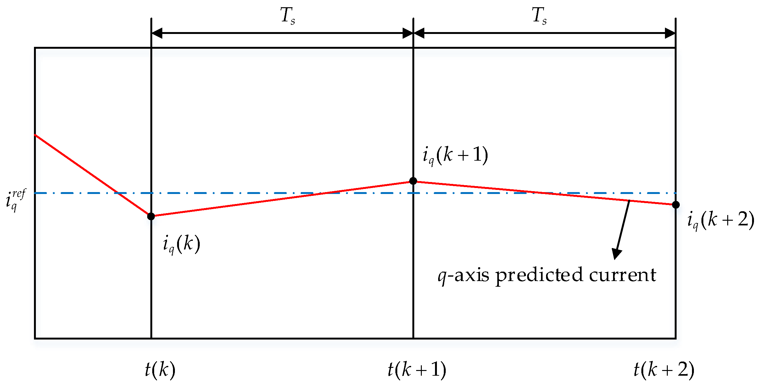
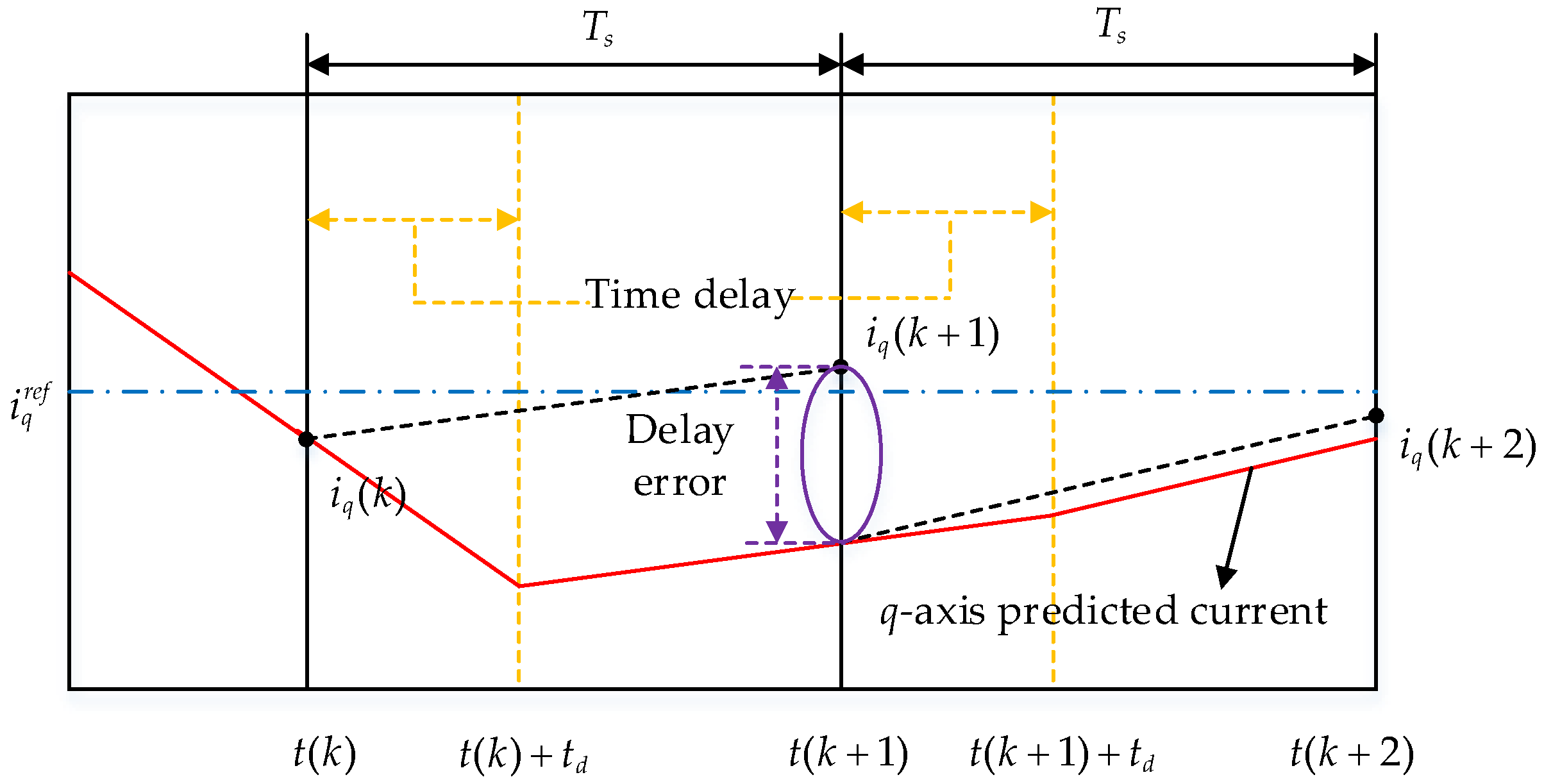
3.2. Model Predictive Current Control Algorithm
- Predictive Current Model
- 2.
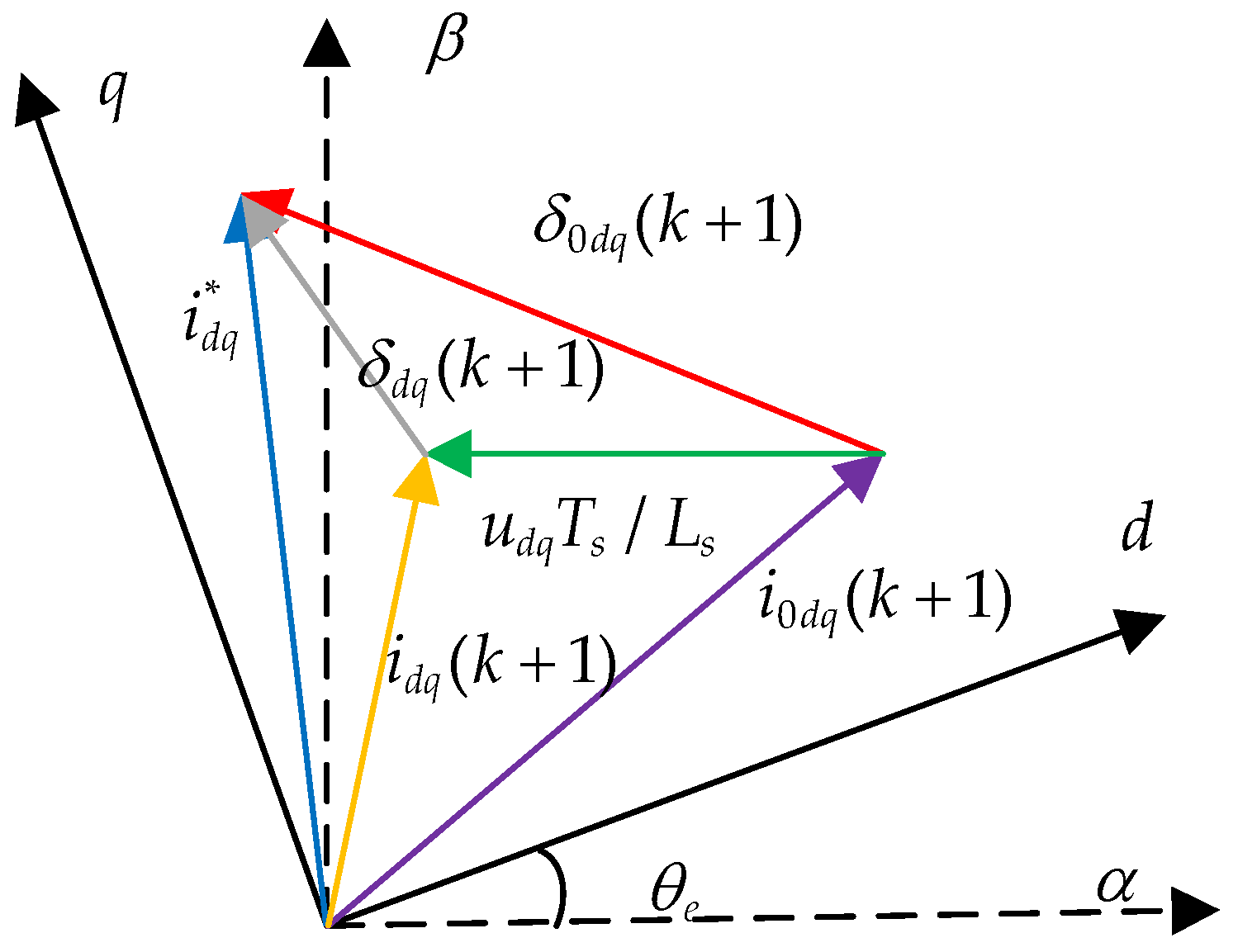
- Analysis and Calculation of Current Error Vector
- 3.
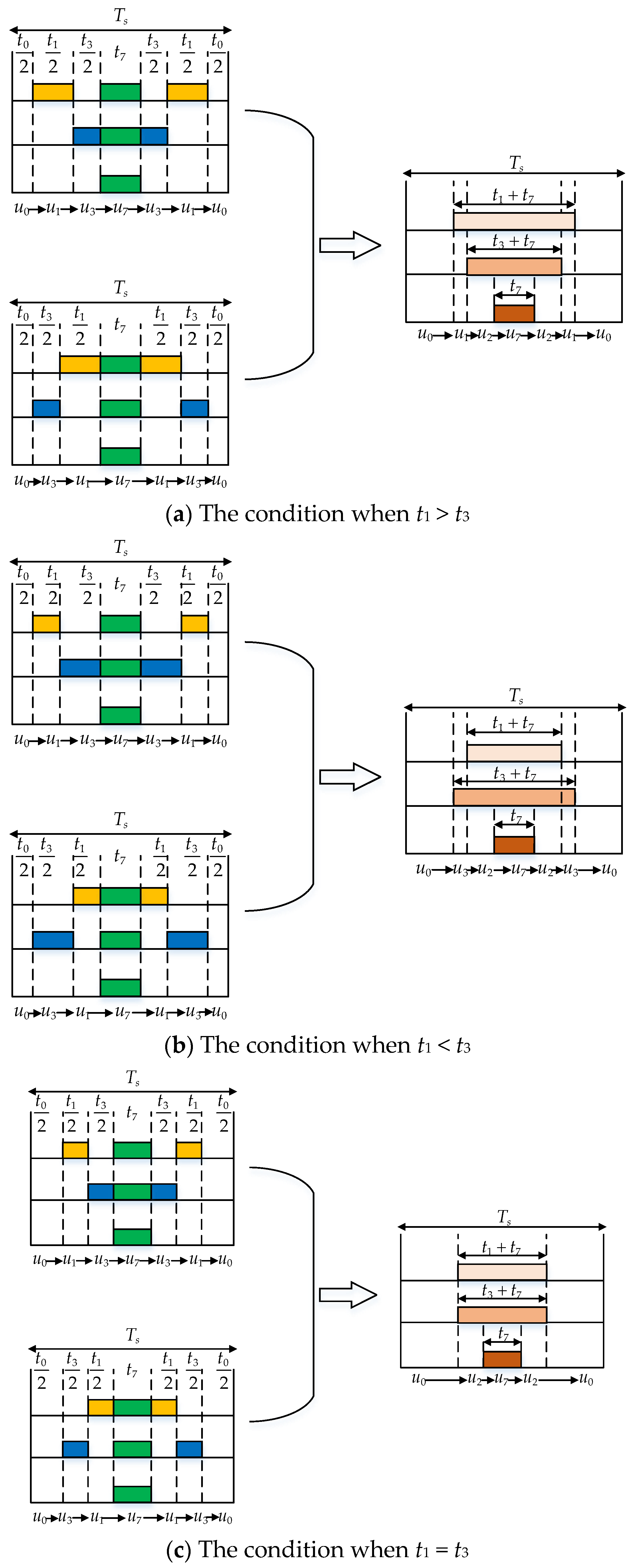
- Determination of Candidate Voltage Vector Combinations
- 4.
- Duty Cycle Calculation and Cost Function Minimization
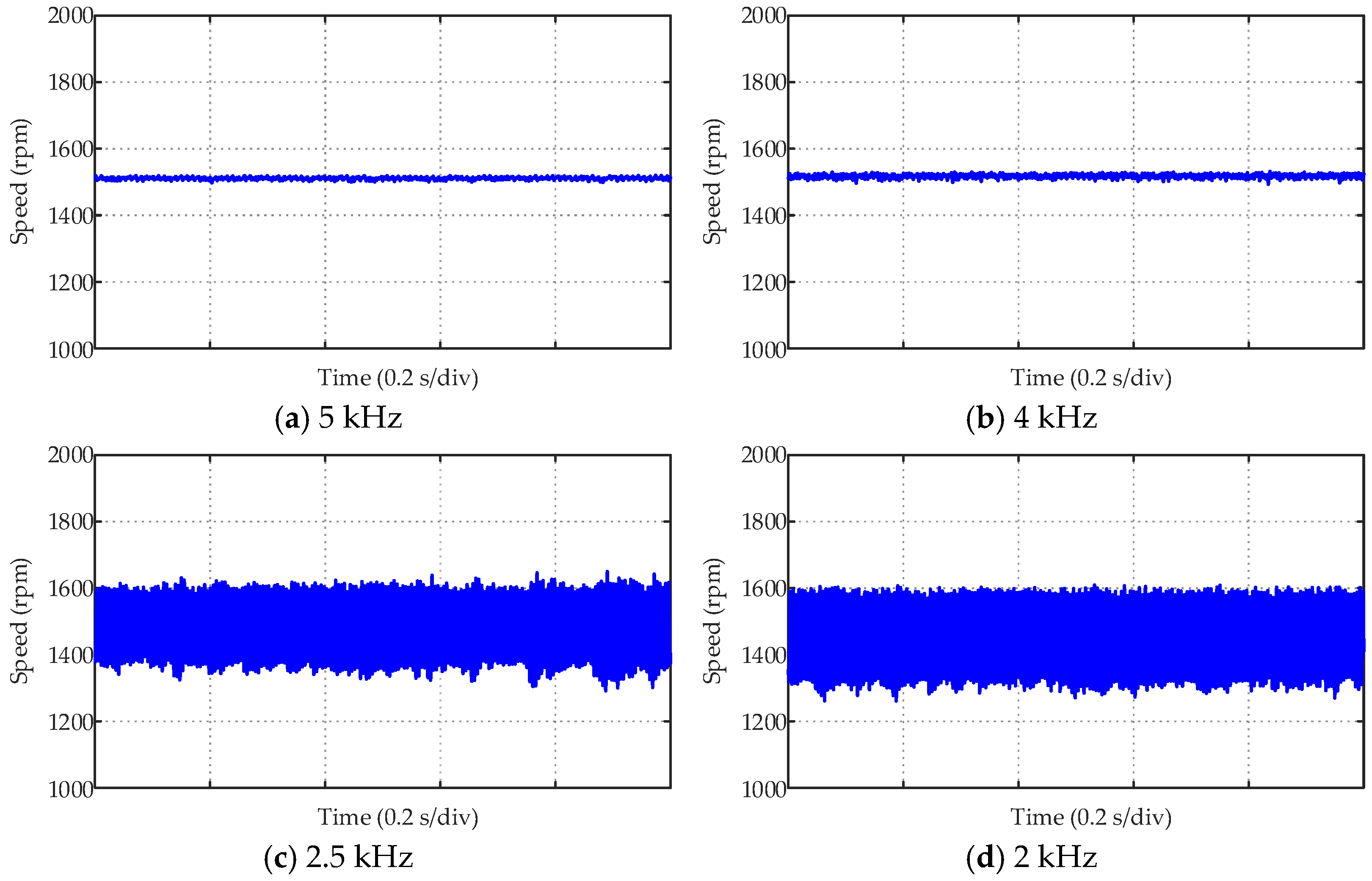
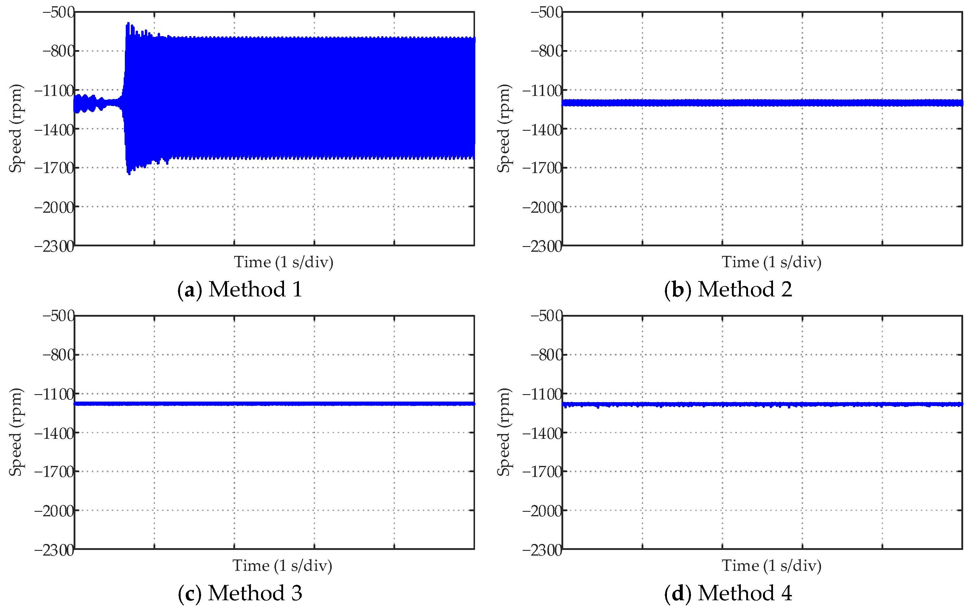
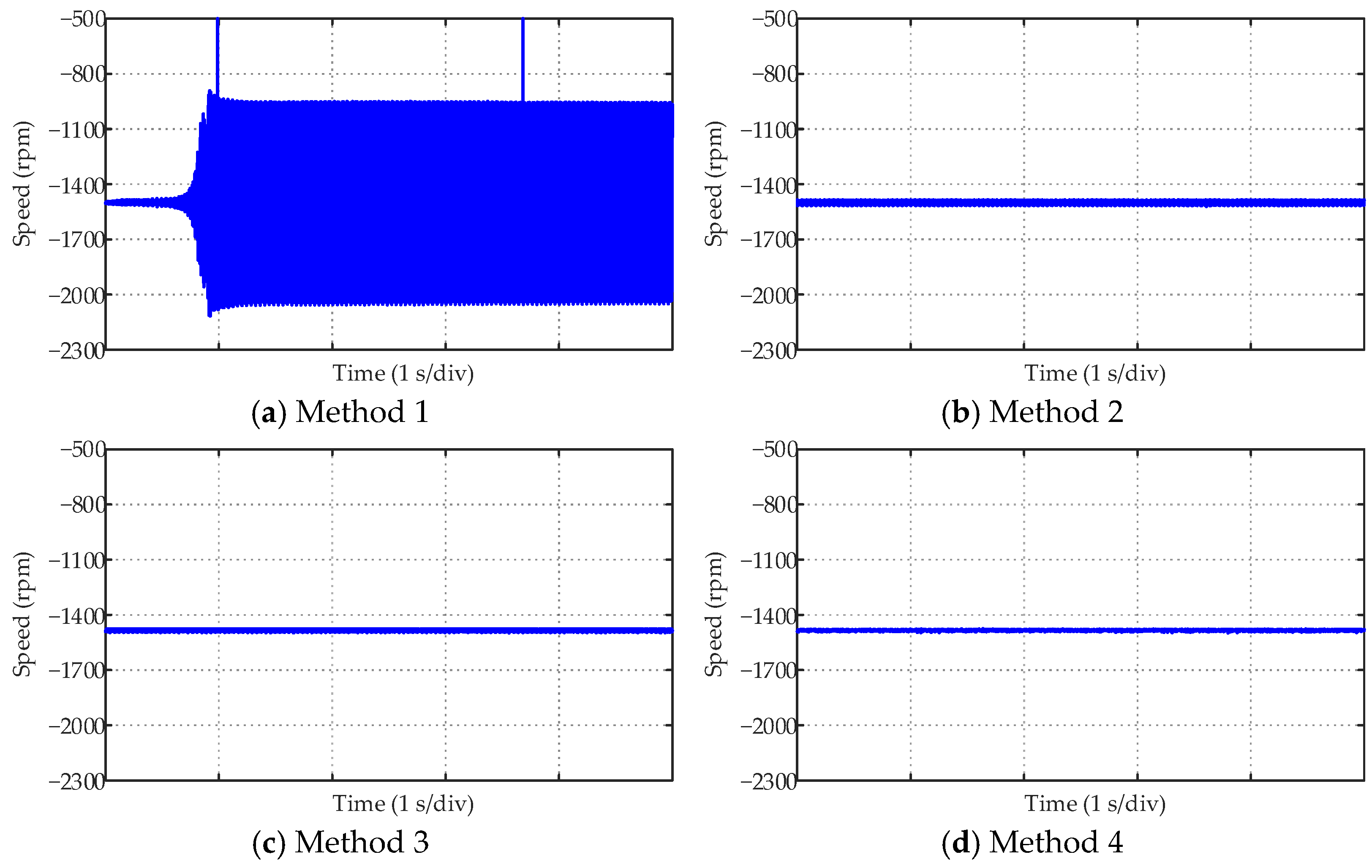
4. Simulation Verification
5. Experimental Test
6. Conclusions
Author Contributions
Funding
Data Availability Statement
Conflicts of Interest
Appendix A


| Method 4 | Without Delay Compensation | With Delay Compensation |
|---|---|---|
| Ripple of 1500 rpm | 3.519 rpm | 5.846 rpm |
| Ripple of 1800 rpm | 7.117 rpm | 16.540 rpm |


References
- Sayed, E.; Abdalmagid, M.; Pietrini, G.; Sa’adeh, N.M.; Callegaro, A.D.; Goldstein, C.; Emadi, A. Review of Electric Machines in More-/Hybrid-/Turbo-Electric Aircraft. IEEE Trans. Transport. Electrific. 2021, 7, 2976–3005. [Google Scholar] [CrossRef]
- Li, X.; Chau, K.T.; Cheng, M. Analysis, design and experimental verification of a field-modulated permanent-magnet machine for direct-drive wind turbines. IET Electr. Power Appl. 2015, 9, 150–159. [Google Scholar] [CrossRef]
- Hong, D.K.; Hwang, W.; Lee, J.Y.; Woo, B.C. Design, Analysis, and Experimental Validation of a Permanent Magnet Synchronous Motor for Articulated Robot Applications. IEEE Trans. Magn. 2018, 54, 8207304. [Google Scholar] [CrossRef]
- Choo, K.M.; Won, C.Y. Design and Analysis of Electrical Braking Torque Limit Trajectory for Regenerative Braking in Electric Vehicles with PMSM Drive Systems. IEEE Trans. Power Electron. 2020, 35, 13308–13321. [Google Scholar] [CrossRef]
- Wu, G.; Huang, S.; Wu, Q.; Zhang, C.; Rong, F.; Hu, Y. Predictive Torque and Stator Flux Control for N∗3-Phase PMSM Drives with Parameter Robustness Improvement. IEEE Trans. Power Electron. 2021, 36, 1970–1983. [Google Scholar] [CrossRef]
- Junejo, A.K.; Xu, W.; Mu, C.; Ismail, M.M.; Liu, Y. Adaptive Speed Control of PMSM Drive System Based a New Sliding-Mode Reaching Law. IEEE Trans. Power Electron. 2020, 35, 12110–12121. [Google Scholar] [CrossRef]
- Chang, Y.C.; Chen, C.H.; Zhu, Z.C.; Huang, Y.W. Speed Control of the Surface-Mounted Permanent-Magnet Synchronous Motor Based on Takagi–Sugeno Fuzzy Models. IEEE Trans. Power Electron. 2016, 31, 6504–6510. [Google Scholar] [CrossRef]
- Wang, Y.; Feng, Y.; Zhang, X.; Liang, J. A New Reaching Law for Antidisturbance Sliding-Mode Control of PMSM Speed Regulation System. IEEE Trans. Power Electron. 2020, 35, 4117–4126. [Google Scholar] [CrossRef]
- Shao, M.; Deng, Y.; Li, H.; Liu, J.; Fei, Q. Robust Speed Control for Permanent Magnet Synchronous Motors Using a Generalized Predictive Controller with a High-Order Terminal Sliding-Mode Observer. IEEE Access 2019, 7, 121540–121551. [Google Scholar] [CrossRef]
- Hu, M.; Hua, W.; Xiao, H.; Wang, Z.; Liu, K.; Cai, K.; Wang, Y. Fast Current Control without Computational Delay by Minimizing Update Latency. IEEE Trans. Power Electron. 2021, 36, 12207–12212. [Google Scholar] [CrossRef]
- Devanshu, A.; Singh, M.; Kumar, N. An Improved Nonlinear Flux Observer Based Sensorless FOC IM Drive with Adaptive Predictive Current Control. IEEE Trans. Power Electron. 2020, 35, 652–666. [Google Scholar] [CrossRef]
- Vafaie, M.H.; Dehkordi, B.M.; Moallem, P.; Kiyoumarsi, A. A New Predictive Direct Torque Control Method for Improving Both Steady-State and Transient-State Operations of the PMSM. IEEE Trans. Power Electron. 2016, 31, 3738–3753. [Google Scholar] [CrossRef]
- An, X.; Liu, G.; Chen, Q.; Zhao, W.; Song, X. Robust Predictive Current Control for Fault-Tolerant Operation of Five-Phase PM Motors Based on Online Stator Inductance Identification. IEEE Trans. Power Electron. 2021, 36, 13162–13175. [Google Scholar] [CrossRef]
- Niu, S.; Luo, Y.; Fu, W.; Zhang, X. Robust Model Predictive Control for a Three-Phase PMSM Motor with Improved Control Precision. IEEE Trans. Ind. Electron. 2021, 68, 838–849. [Google Scholar] [CrossRef]
- Chen, W.; Zeng, S.; Zhang, G.; Shi, T.; Xia, C. A Modified Double Vectors Model Predictive Torque Control of Permanent Magnet Synchronous Motor. IEEE Trans. Power Electron. 2019, 34, 11419–11428. [Google Scholar] [CrossRef]
- Morel, F.; Lin-Shi, X.; Rétif, J.M.; Allard, B.; Buttay, C. A Comparative Study of Predictive Current Control Schemes for a Permanent-Magnet Synchronous Machine Drive. IEEE Trans. Ind. Electron. 2009, 56, 2715–2728. [Google Scholar] [CrossRef]
- Zhang, Y.; Yang, H. Generalized Two-Vector-Based Model-Predictive Torque Control of Induction Motor Drives. IEEE Trans. Power Electron. 2015, 30, 3818–3829. [Google Scholar] [CrossRef]
- Zhang, Y.; Yang, H. Two-Vector-Based Model Predictive Torque Control Without Weighting Factors for Induction Motor Drives. IEEE Trans. Power Electron. 2016, 31, 1381–1390. [Google Scholar] [CrossRef]
- Zhang, X.; Hou, B. Double Vectors Model Predictive Torque Control Without Weighting Factor Based on Voltage Tracking Error. IEEE Trans. Power Electron. 2018, 33, 2368–2380. [Google Scholar] [CrossRef]
- Xu, Y.; Wang, J.; Zhang, B.; Zhou, Q. Three-Vector-Based Model Predictive Current Control for Permanent Magnet Synchronous Motor. Trans. China Electrotech. Soc. 2018, 33, 980–988. [Google Scholar]
- Xu, Y.; Wang, J.; Zhou, Q.; Zhang, B. Double Optimization Three-vector-based Model Predictive Current Control for Permanent Magnet Synchronous Motors. Proc. CSEE 2018, 38, 1857–1864+1923. [Google Scholar]
- Kang, S.W.; Soh, J.H.; Kim, R.Y. Symmetrical Three-Vector-Based Model Predictive Control with Deadbeat Solution for IPMSM in Rotating Reference Frame. IEEE Trans. Ind. Electron. 2020, 67, 159–168. [Google Scholar] [CrossRef]
- Xu, B.; Jiang, Q.; Ji, W.; Ding, S. An Improved Three-Vector-Based Model Predictive Current Control Method for Surface-Mounted PMSM Drives. IEEE Trans. Transport. Electrific. 2022, 8, 4418–4430. [Google Scholar] [CrossRef]
- Li, X.; Xue, Z.; Zhang, L.; Hua, W. A Low-Complexity Three-Vector-Based Model Predictive Torque Control for SPMSM. IEEE Trans. Power Electron. 2021, 36, 13002–13012. [Google Scholar] [CrossRef]
- Xu, Y.; Ding, X.; Wang, J.; Li, Y. Three-vector-based low-complexity model predictive current control with reduced steady-state current error for permanent magnet synchronous motor. IET Electr. Power Appl. 2020, 14, 305–315. [Google Scholar] [CrossRef]
- Chen, R.; Shu, H.; Zhai, K. Low-Complexity Three-Vector Model Predictive Current Control with Fixed Switching Frequency for PMSM. In Proceedings of the CSEE, Winnipeg, MB, Canada, 1 June 2023. early access. [Google Scholar]
- Li, X.; Tian, W.; Gao, X.; Yang, Q.; Kennel, R. A Generalized Observer-Based Robust Predictive Current Control Strategy for PMSM Drive System. IEEE Trans. Ind. Electron. 2022, 69, 1322–1332. [Google Scholar] [CrossRef]
- Yu, K.; Wang, Z.; Hua, W.; Cheng, M. Robust Cascaded Deadbeat Predictive Control for Dual Three-Phase Variable-Flux PMSM Considering Intrinsic Delay in Speed Loop. IEEE Trans. Ind. Electron. 2022, 69, 12107–12118. [Google Scholar] [CrossRef]
- Guo, T.; Wang, Z.; Zhang, H.; Jiang, X.; Tian, L. Cascaded predictive Speed Control Optimization Method based on Fuzzy Controller. In Proceedings of the 6th IEEE International Conference on Predictive Control of Electrical Drives and Power Electronics, PRECEDE 2021, Jinan, China, 20–22 November 2021; pp. 328–335. [Google Scholar]
- Liu, J.; Ge, Z.; Wu, X.; Wu, G.; Xiao, S.; Huang, K. Predictive Current Control of Permanent Magnet Synchronous Motor Based on Duty-cycle Modulation. Proc. CSEE 2020, 40, 3319–3328. [Google Scholar]
- Xiao, X.; Zhang, Y.; Wang, J.; Du, H. An Improved Model Predictive Control Scheme for the PWM Rectifier-Inverter System Based on Power-Balancing Mechanism. IEEE Trans. Ind. Electron. 2016, 63, 5197–5208. [Google Scholar] [CrossRef]
- Han, Y.; Gong, C.; Yan, L.; Wen, H.; Wang, Y.; Shen, K. Multiobjective Finite Control Set Model Predictive Control Using Novel Delay Compensation Technique for PMSM. IEEE Trans. Power Electron. 2020, 35, 11193–11204. [Google Scholar] [CrossRef]


| Parameters | Symbol | Value |
|---|---|---|
| Rated torque | ||
| Rated speed | ||
| Stator inductance | ||
| Stator phase resistance | ||
| Number of pole pairs | ||
| Flux linkage of permanent magnets | ||
| DC-bus voltage | ||
| Rotational inertia |
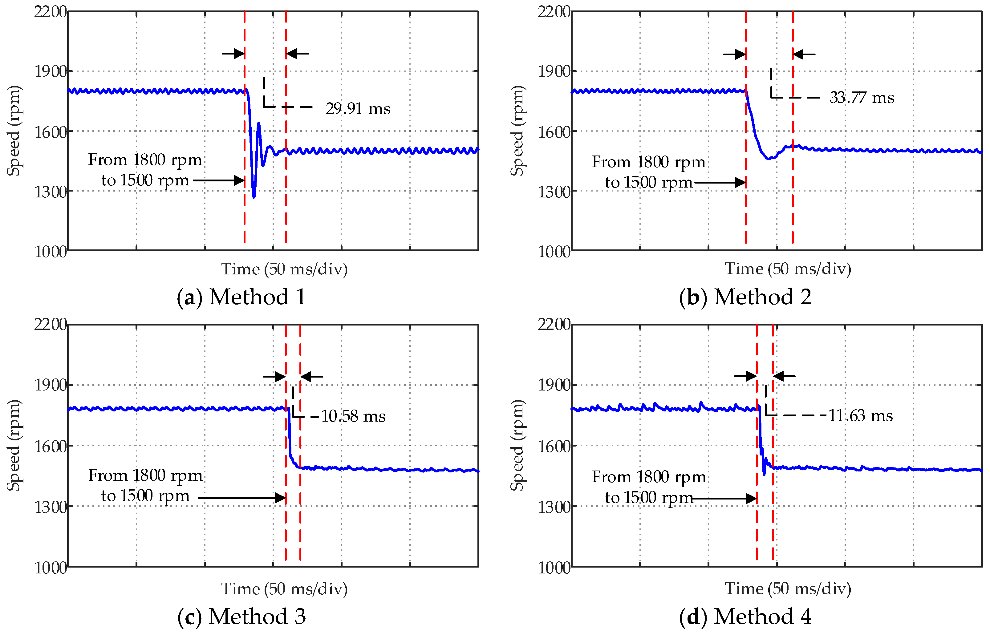
| Method (1~4) | Starting Overshoot | Response Time | Speed Drop after Loading | Speed Recovery Time after Loading |
|---|---|---|---|---|
| Method 1 | 15.9% | 0.223 s | 101.6 rpm | 0.170 s |
| Method 2 | 13.2% | 0.134 s | 23.1 rpm | 0.064 s |
| Method 3 | 0 | 0.021 s | 22.8 rpm | 0.063 s |
| Method 4 | 0 | 0.021 s | 22.8 rpm | 0.063 s |
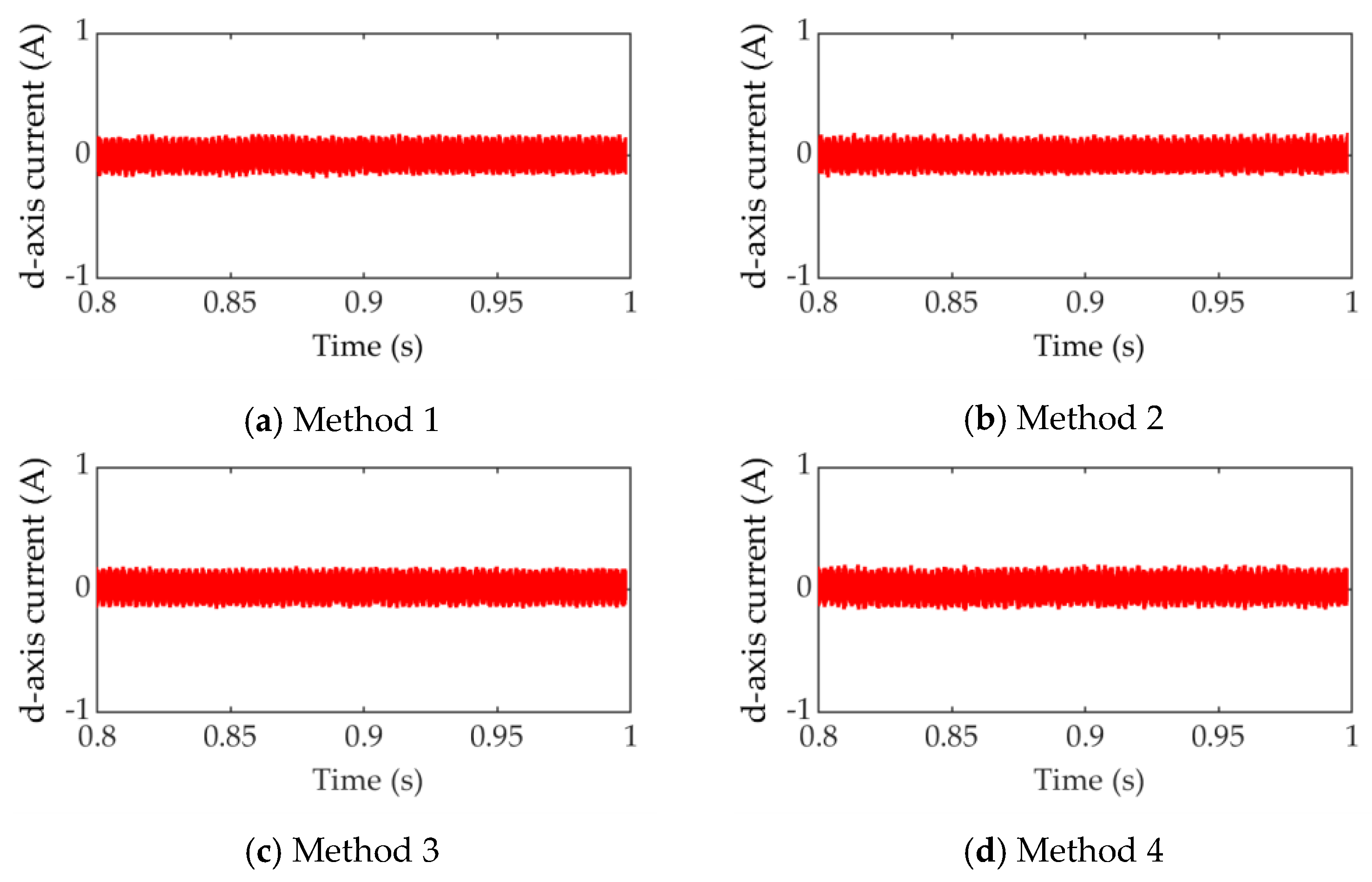
| Method (1~4) | Method 1 | Method 2 | Method 3 | Method 4 |
|---|---|---|---|---|
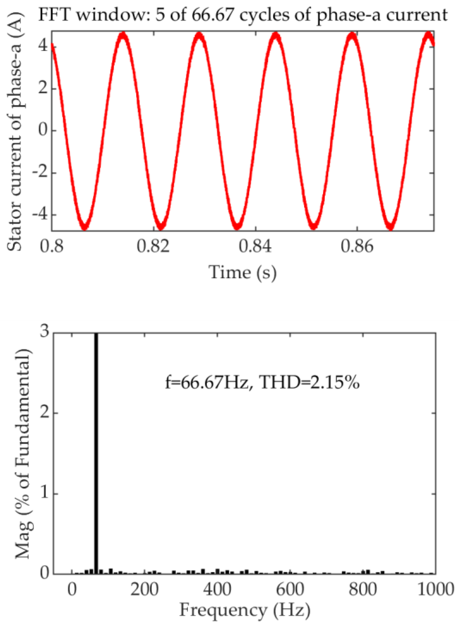
| THD of phase-a | 2.12% | 2.12% | 2.05% | 2.15% |
| Parameters | Symbol | Value |
|---|---|---|
| Rated torque | ||
| Rated speed | ||
| Stator inductance | ||
| Stator phase resistance | ||
| Number of pole pairs | ||
| Flux linkage of permanent magnets | ||
| DC-bus voltage | ||
| Rotational inertia |
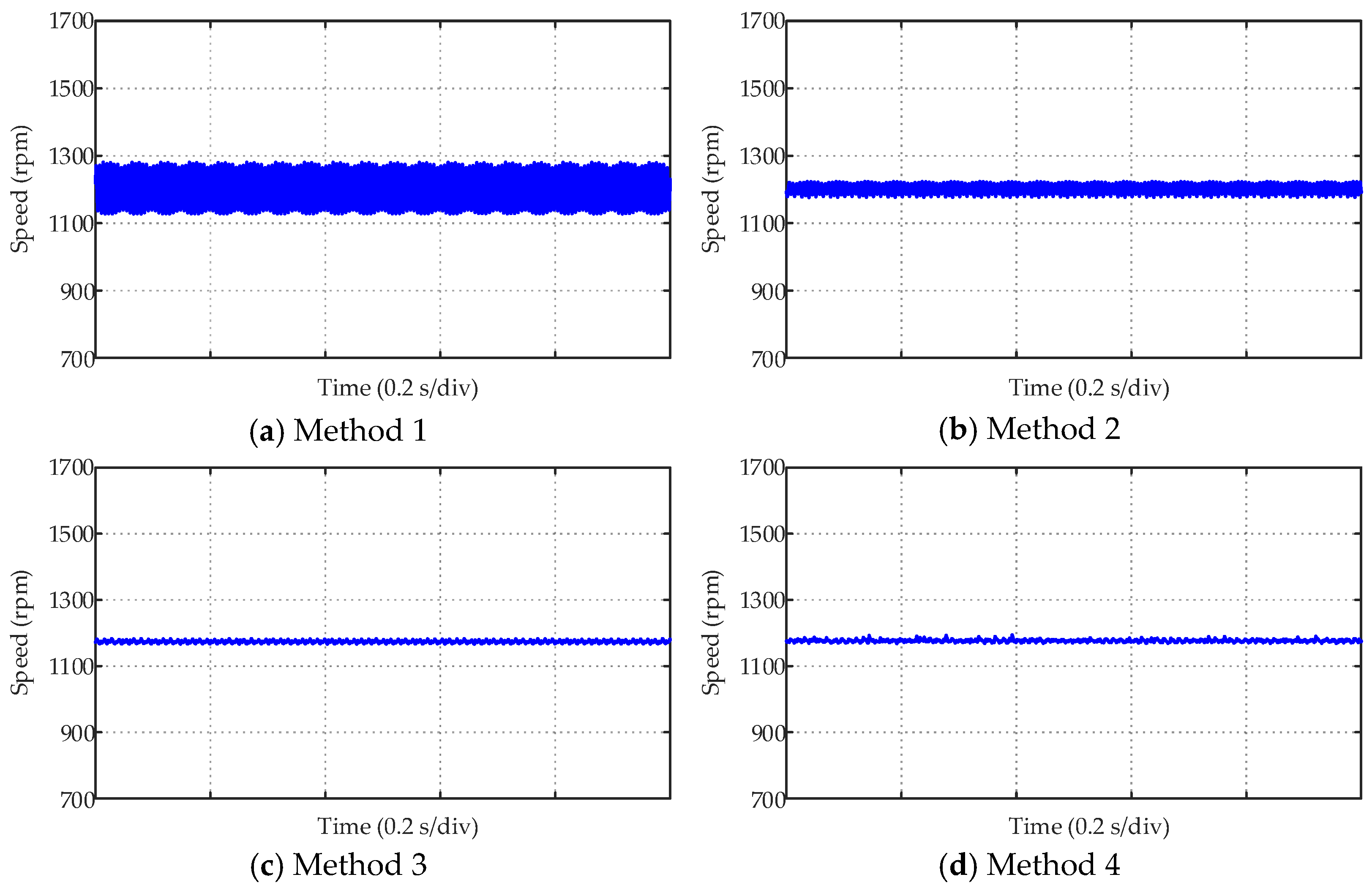
| Method (1~4) | Method 1 | Method 2 | Method 3 | Method 4 |
|---|---|---|---|---|
| Ripple of 1800 rpm | 6.160 rpm | 4.846 rpm | 4.558 rpm | 7.117 rpm |
| Ripple of 1500 rpm | 10.340 rpm | 6.176 rpm | 3.121 rpm | 3.519 rpm |
| Ripple of 1200 rpm | 49.579 rpm | 13.938 rpm | 3.719 rpm | 3.567 rpm |
| Method (3~4) | Method 3 | Method 4 |
|---|---|---|
| Turnaround time | 19.96 μs | 13.48 μs |
Disclaimer/Publisher’s Note: The statements, opinions and data contained in all publications are solely those of the individual author(s) and contributor(s) and not of MDPI and/or the editor(s). MDPI and/or the editor(s) disclaim responsibility for any injury to people or property resulting from any ideas, methods, instructions or products referred to in the content. |
© 2023 by the authors. Licensee MDPI, Basel, Switzerland. This article is an open access article distributed under the terms and conditions of the Creative Commons Attribution (CC BY) license (https://creativecommons.org/licenses/by/4.0/).
Share and Cite
Meng, Q.; Bao, G. A Novel Low-Complexity Cascaded Model Predictive Control Method for PMSM. Actuators 2023, 12, 349. https://doi.org/10.3390/act12090349
Meng Q, Bao G. A Novel Low-Complexity Cascaded Model Predictive Control Method for PMSM. Actuators. 2023; 12(9):349. https://doi.org/10.3390/act12090349
Chicago/Turabian StyleMeng, Qingcheng, and Guangqing Bao. 2023. "A Novel Low-Complexity Cascaded Model Predictive Control Method for PMSM" Actuators 12, no. 9: 349. https://doi.org/10.3390/act12090349