Design and Optimization of a Novel Electronic Mechanical Brake Actuator Based on Cam

Abstract

The electronic mechanical brake (EMB) is considered an ideal actuator for brake-by-wire systems. We applied the negative radius roller cam mechanism as the clamping mechanism of the EMB, solving the problem of large size, poor load-bearing capacity, and the inefficiency of the existing EMBs. When designing a cam as a clamping transmission mechanism, it is necessary to take the pressure angle, contact stress, motion law, etc., as goals and constraints. Existing design methods cannot easily solve this problem. Therefore, we propose a new analysis method from the cam profile and combine it with an improved particle swarm optimization (PSO) algorithm to design the cam profiles. This method can handle various complex goals and constraints of the EMB and obtain the required negative radius roller cam profile. Finally, the logical consistency of the profile-based analysis method was verified, and the EMB design objectives and accuracy were compared using ADAMS. Under the same conditions, the result showed that the optimized cam mechanism requires only 40.52% motor power and only 65.65% clearance elimination time compared to the EMB with the lead screw mechanism.

1. Introduction

Autonomous driving is a popular scenario for the application of artificial intelligence technology, and vehicle chassis control by wire is an inevitable requirement for vehicles to achieve autonomous driving [1,2]. The electronic mechanical brake (EMB) is considered one of the most-ideal actuators for achieving vehicle brake control by wire [3,4].

Compared to traditional hydraulic brakes or electronic hydraulic brakes (EHBs) [5], it has many advantages. Firstly, the pumps, pipelines, valves, and other components of the hydraulic system have complex structures and risks of leakage, while pure mechanical transmission methods are more reliable. Secondly, the EHB’s control-by-wire action is usually on/off valves, and the control output is discrete [6]. However, the EMB can achieve continuous adjustment, making the control execution performance superior [7,8].

The EMB actuators generally need to convert the rotational motion of the motor into linear motion similar to a piston cylinder to compress the friction plate onto the brake disc to achieve vehicle braking [9]. The existing actuators include screw mechanisms [10,11], linkage mechanisms [12], and cam mechanisms [13,14]. Besides, the brakes are installed inside the wheel rim, with very limited space, and need to withstand a few tons of force, so the existing mechanisms generally have problems such as poor load-bearing capacity, large size, and low efficiency.

The screw mechanism can be divided into the ball screw mechanism and sliding screw mechanism. The screw converts the relative rotation between the nut and the screw into relative movement through the principle of thread transmission. Balls are installed between the screw and nut of the ball screw, which convert the relative sliding into rolling, improving efficiency and reducing wear. However, compared to sliding screws, ball screws have become more complex in structure and more difficult to process and have an increased volume, but the load-bearing capacity is reduced. In addition, the lead of the ball screw is limited by the size of the ball compared to the sliding screw, resulting in a small transmission ratio and the need for a large speed-ratio-reduction mechanism. However, the application of sliding screws in the EMB is also limited due to efficiency and wear issues.

The principle of the linkage mechanism for clamping is to use the moving pair at the end of the mechanism or approximate movement with the swing of the large arm length. However, the design of the linkage mechanism itself is relatively complex, and the characteristics of the transmission are closely related to the length of the rod. It is very difficult to design ideal transmission characteristics in a limited space. Because the clamping force required is very large and the rods usually bear a bending force, the load on some kinematic pair is also very large. To ensure strength, its structural dimensions will become larger. This limits its application on the EMB.

The principle of the cam mechanism to achieve motion conversion is cam pairs. Due to the characteristic of high contact pairs, general cam mechanics are usually not used in situations with particularly high loads.

The negative radius roller cam mechanism is different from general cam mechanisms, and it has some attractive advantages for use on EMBs:

• Because the contact surface between the cam and the roller is internally tangent, the negative radius roller cam mechanism has low contact stress and high bearing capacity [15].
• Because the rollers are achieved through rolling bearings, there are no relatively sliding components in the negative radius roller cam mechanism, which has higher efficiency and less wear.
• In terms of design, compared to the screw and the linkage mechanism, the cam mechanism is flexible to design the transmission relationship and the size changes very little.

The traditional design of the cam mechanism is often focused on the motion law of the follower [16,17]. Starting from the motion law, the method of using differential geometry and other methods to analytically solve the cam profile are relatively mature [18]. For applications that only require specific movements such as push, return, far rest, and near rest, this method can effectively solve most problems [19]. However, in the EMB, because the input motion is arbitrary, the output motion pattern is not the most-direct design goal, and simply ensuring whether there is an impact is not enough [20,21]. The cam mechanism in the EMB acts as a transmission mechanism, having other design goals we need to care about [22]. The traditional design of the cam mechanism is often focused on the motion law of the follower [16,17]. Starting from the motion law, the method of using differential geometry and other methods to analytically solve the cam profile are relatively mature [18]. For applications that only require specific movements such as push, return, far rest, and near rest, this method can effectively solve most problems [19]. However, in the EMB, because the input motion is arbitrary, the output motion pattern is not the most-direct design goal, and simply ensuring whether there is an impact is not enough [20,21]. The cam mechanism in the EMB acts as a transmission mechanism, having other design goals we need to care about [22].

Considering the application scenarios of cams in complex situations such as high-speed and specific loads [23,24], relevant scholars have analyzed and studied the performance of cam transmission. Some scholars have studied the influence of different variable offset on the pressure angle [25]; studied the influence of different motion laws (such as sinusoidal motion law, cycloidal motion law, 3-4-5 motion law, etc.) on contact stress [26]; as well as the changes of the pressure angle and curvature radius under Bézier curves of different orders [27]. These methods are all based on motion laws, which have good guiding significance for designing cam mechanisms. However, most of the above methods are the summary of the laws under the condition of controlling univariate changes, or only a part of the parameters of the cam mechanism are included, making it difficult to achieve ideal results for complex design goals.

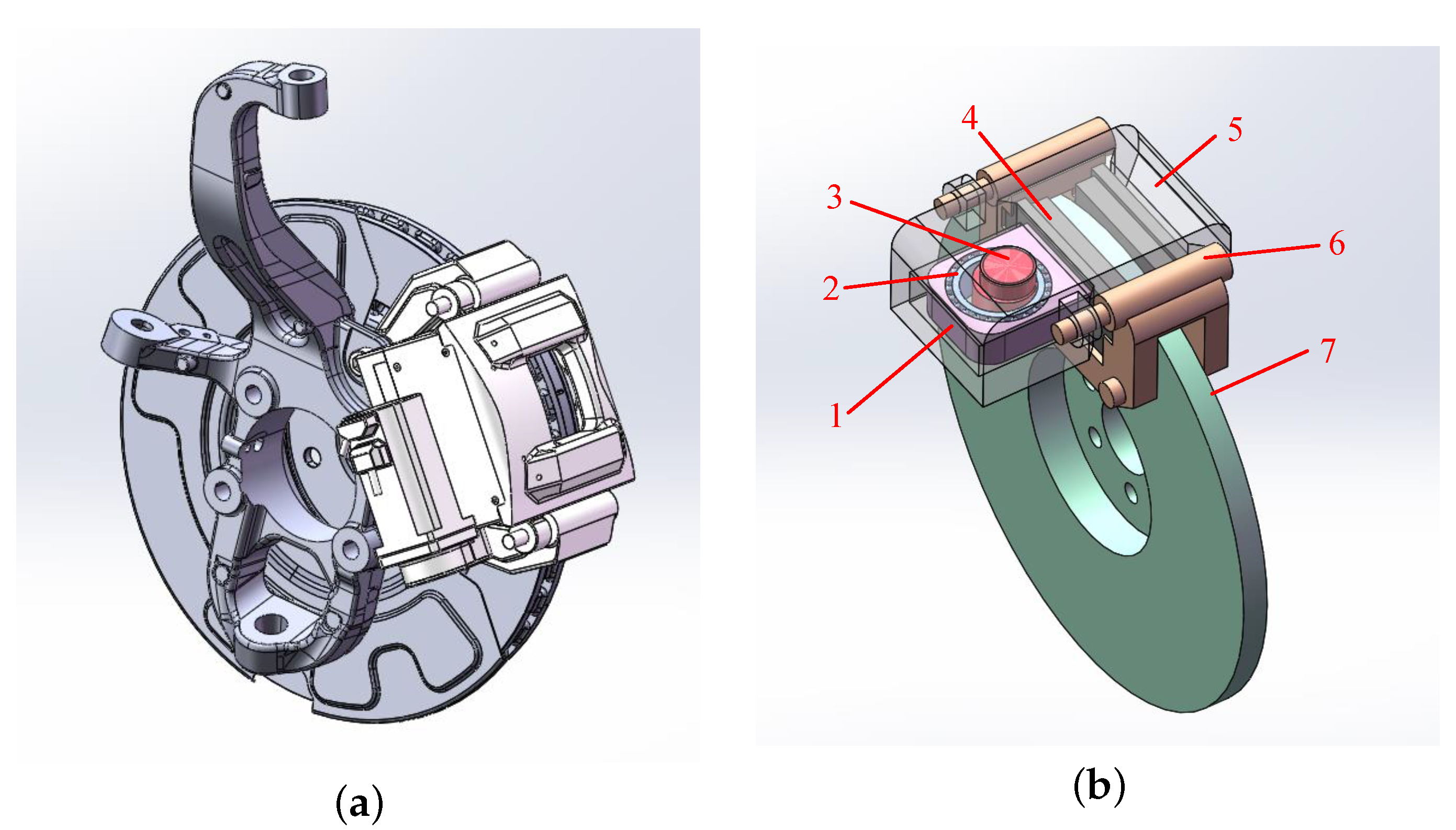
The research question in this article is to design a novel EMB. It has advantages over existing configuration of EMBs. By optimizing the design of the profile, the transmission characteristics of the cam mechanism can better comply with the EMB working conditions. The main contributions of this article include the following:

• We propose a novel EMB based on negative radius roller cam mechanisms;
• We propose a profile-based analysis method for negative radius roller cam mechanisms. The advantage of this method is that it can directly obtain most parameters using relatively simple expressions;
• We find a set of simple and universal cam mechanism design parameters to optimize the design;
• We improved the particle swarm optimization (PSO) algorithm for designing cam profiles by designing correction algorithms. The correction algorithms we propose can guide particles to meet constraints and accelerate algorithm convergence.

Section 2 of this article will elaborate the design question of the cam profiles faced by the EMB and derive the motion laws and other characteristics of negative radius roller cam mechanisms from its profile; Section 3 provides the specific process of solving the cam profiles using improved PSO algorithm; Section 4 discusses the results obtained using the method presented in this article and compares and verifies the design results using ADAMS.

2. Problem Posing and Profile-Based Analysis Method

2.1. EMB Layout Scheme Based on Negative Radius Roller Cam Mechanism

The schematic diagram of the negative radius roller cam mechanism is shown in Figure 1a. The red and orange curves in the figure form the two profiles of the cam, while the green circles represent the inner and outer rings of the rolling bearing as the follower. The cam rotates around the center of rotation, while the driven bearing can only move in the vertical direction. The positive radius roller cam mechanism (the roller cam mechanism in the usual sense) is shown in Figure 1b. The biggest difference between a negative radius roller cam mechanism and a positive radius roller cam mechanism is whether the cam profile and rollers are inscribed or circumscribed. This affects the magnitude of contact stress and the placement of the moving pair.

The layout structure of the EMB based on a negative radius cam mechanism is shown in Figure 2. Figure 2a is the assembly appearance, and the detailed implementation cases can be found in our patent application [28,29]. Figure 2b is the schematic diagram of the core cam mechanism. As shown in Figure 2b, the driven bearing is installed inside the driven bracket, which can move in a straight line within the caliper housing. The camshaft passes through the driven bearing, and when the camshaft rotates, its profile contacts the inner ring of the driven bearing. The driven bracket pushes the friction plate against the brake disc. The caliper housing and friction plate are both installed on the caliper bracket and can move horizontally relative to the caliper bracket. The caliper bracket is usually installed on the steering knuckle or the vehicle axle.

2.2. Analysis of Design Issues

In the application scenario of the EMB, we hope to design a negative radius roller cam mechanism with smooth transmission, a small pressure angle, high efficiency, an appropriate curvature radius, etc. However, in fact, the pressure angle, contact stress, and distortion of the cam mechanism are all related to the motion law of the cam. In theory, for a clear design requirement goal function, there exists an optimal follower motion law and offset distance parameters that can meet the requirements.

Specifically, if the displacement motion law of the follower is $s\left(\phi \right)$, then the velocity motion law is $ds/d\phi$ and the acceleration motion law is $d^{2}s/d{\phi }^2$. For the negative radius roller cam mechanism, its pressure angle formula [30] can be obtained through the instantaneous center method:

$$\alpha =arctan\left(\frac{\left|ds/d\phi -e\right|}{s_0-s}\right)$$

(1)

where $s_0=r_g-\sqrt{r_{st}^2-e^2}$, $r_g$ represents the inner radius of the roller, $r_{st}$ represents the distance from the tangent point to the center of rotation when the cam is in its initial position, and e represents the offset. It can be seen that the pressure angle mainly depends on the speed motion law, displacement motion law, and the offset.

If the characteristic of the load is known as $F_{ca}\left(s\right)$, then based on the instantaneous power being equal, the relationship between the torque of the driving actuator and the load is

$$F_{ca}\left(s\right)ds=T\left(\phi \right)d\phi$$

(2)

Therefore, the magnitude of the driving torque or “transmission ratio” is also related to the speed motion law.

As for distortion and contact stress, they are often related to the curvature radius of the cam working profile. It is difficult to directly derive the curvature radius of the profile through the laws of motion. Assuming that the parameter expression of the cam working profile regarding the cam rotation angle $\phi$ can be obtained through analytical methods as $x\left(\phi \right)$ and $y\left(\phi \right)$, the curvature radius formula of the parameter equation curve is

$$\rho \left(\phi \right)=\frac{{\left(x^{\prime }{\left(\phi \right)}^2+y^{\prime }{\left(\phi \right)}^2\right)}^{\frac{3}{2}}}{\left|x^{\prime }\left(\phi \right)y^{\prime \prime }\left(\phi \right)-y^{\prime }\left(\phi \right)x^{\prime \prime }\left(\phi \right)\right|}$$

(3)

According to the formula for solving the envelope curve [31], the cam working profile $x\left(\phi \right)$ and $y\left(\phi \right)$ are expressions of $s\left(\phi \right)$ and $ds/d\phi$ and contain trigonometric functions. Therefore, the radius of curvature of the profile is a nonlinear expression containing at least the third-order motion law of the cam.

Therefore, if the pressure angle, contact stress, etc., need to be taken as the design goal in the process of cam profile design and the profile distortion and other problems need to be taken as constraints, the problem of comprehensively solving the optimal motion law $s^{*}\left(\phi \right)$ is a functional extreme value problem under nonlinear constraints. Obviously, the analytical solution to this problem is very difficult. Because the curvature radius and other expressions of the profile need to be indirectly obtained from the theoretical profile and envelope curve based on the motion law, numerical solution is also quite difficult. Therefore, if these goals and constraints are not urgent, traditional methods will choose to directly give a certain motion law.

In view of the above problems, this paper proposes a profile-based analysis method, that is starting from the cam profile under polar coordinates to analyze the motion law of the cam mechanism in the contact process, as well as the pressure angle, curvature radius, etc., then use the improved PSO algorithm solving the cam profile to meet the requirements. The basic framework of the two methods is shown in Figure 3.

2.3. Profile-Based Analysis Method

The specific analysis of the cam profile is shown in Figure 4, where the red curve represents a segment of the cam profile and the cam rotates clockwise, as shown in the diagram. The blue curve is a segment of the inner ring of the driven bearing, and the radius of the circle is $r_g$. The blue dashed line is the axis of the follower movement. Among them, O is the rotation center of the cam; A is the center of the bearing; B is the tangent point between the cam profile and the inner ring of the driven bearing. $OC$ is perpendicular to the moving axis and perpendicular to C, and the length of $OC$ is the offset distance e. $OD$ is perpendicular to $AB$ and perpendicular to D. The points E and F represent the intersection of $AC$ and $AB$ with the horizontal axis of the coordinate system.

Let the expression of the cam profile in polar coordinates be $r\left(\theta \right)$, abbreviated as r, which is the length of $OB$ in Figure 4. Then, Point B on the profile can be expressed as

$$\left\{\begin{array}{c}{x}_B=rcos\left(\theta \right)\\ y_B=rsin\left(\theta \right)\end{array}\right.$$

(4)

Calculate the slope of the tangent line at Point B on the cam profile:

$$k_B=\frac{dy}{dx}=\frac{dy}{d\theta }\frac{d\theta }{dx}=\frac{\dot{r}sin\theta +rcos\theta }{\dot{r}cos\theta -rsin\theta }$$

(5)

where $\dot{r}=dr/d\theta$, then the slope of the normal is

$$k_{Bf}=-\frac{1}{k_B}$$

(6)

The equation for the normal $AB$ is

$$y-y_B=k_{Bf}\left(x-x_B\right)$$

(7)

The distance from the origin to the normal $AB$ is defined as the normal force arm l

$$l:=\left|OD\right|=\frac{\left|y_B-k_{Bf}{x}_B\right|}{\sqrt{1+k_{Bf}^2}}$$

(8)

The distance between the center of cam rotation and the center of the driven bearing is obtained by using geometric relationships (see Appendix A for details):

$$\left|OA\right|=\sqrt{r^2+r_g^2-2r_g\sqrt{r^2-l^2}}$$

(9)

Finally, the length $\left|AC\right|=\sqrt{{\left|OA\right|}^2-{\left|OC\right|}^2}$ is obtained through an Rt$▵OCA$, which is

$$h:=\left|AC\right|=\sqrt{r^2+r_g^2-2r_g\sqrt{r^2-l^2}-e^2}$$

(10)

Starting from the initial position, the corresponding follower lifts at different profile angles $\theta$ is

$$s=h\left({\theta }_0\right)-h\left(\theta \right)$$

(11)

The movement direction of the driven bearing is in the $AC$ direction, and the contact force between the driven bearing and the cam follows their common normal direction. Therefore, the contact force is

$$F_B=F/cos\alpha$$

(12)

where $\alpha$ is the pressure angle of the follower.

According to the different positions of tangent Point B, the relative positions of perpendicular foot D and center A will change. Using Rt$\Delta OCA$ and Rt$\Delta ODA$, the pressure angle at two relative positions is expressed as

$$\alpha =\left\{\begin{array}{cc}arcsin\left(\frac{e}{\left|OA\right|}\right)-arcsin\left(\frac{l}{\left|OA\right|}\right)& r_g\ge \sqrt{r^2-l^2}\\ arcsin\left(\frac{e}{\left|OA\right|}\right)+arcsin\left(\frac{l}{\left|OA\right|}\right)-\pi & r_g<\sqrt{r^2-l^2}\end{array}\right.$$

(13)

where the negative value of the pressure angle is opposite the direction shown in Figure 4, on the right side of the common normal line.

The cam pushes the driven bearing to move, and the torque is

$$T=F_B·l$$

(14)

Calculate the contact stress at each point during cam operation according to the Hertz formula:

$${\sigma }_H=Z_E\sqrt{\frac{F_B}{L{\rho }_{\epsilon }}}$$

(15)

where L represents the length of the cam contact line; $Z_E$ is a coefficient related to the material; ${\rho }_{\epsilon }=\frac{{\rho }_1{\rho }_2}{{\rho }_1-{\rho }_2}$ is the comprehensive curvature radius; and the curvature radius of the roller ${\rho }_1=r_g$. For the curvature radius of the cam in polar coordinates, the formula is

$${\rho }_2=\frac{{\left(r^2+{\dot{r}}^2\right)}^{\frac{3}{2}}}{\left|r^2+2{\dot{r}}^2-r\ddot{r}\right|}$$

(16)

where $\ddot{r}=d^{2}r/d{\theta }^2$.

Finally, the above analysis is based on each point on the profile. The angle between two different points on the profile and the line connecting the cam rotation center is represented by $\theta$, which is called the profile angle. During the process of cam rotation, the angle at which the cam rotates around the center of rotation is called the rotation angle, denoted by $\phi$. Because the relative position of the contact point between the cam and the follower changes during the rotation of the cam, the rotation angle and the profile angle are not the same, as shown in Figure 5. Assuming that both the rotation angle and the profile angle are based on the position of the horizontal axis in Figure 4, then based on the geometric relationship (see Appendix A for details):

$$\phi =\theta -arcsin\left(\frac{l}{r}\right)+\alpha$$

(17)

3. Cam Design

3.1. Characteristics of Caliper Device

The caliper device is the final executing device for braking, so the mechanical characteristics of the caliper, friction plate, and brake disc will be an important basis for designing the transmission characteristics. To ensure that there is no contact between the friction plate and the brake disc during non-braking, a certain gap needs to be left between the friction plate and the brake disc [32]. In addition, relevant studies have shown that there is a nonlinear relationship between clamping force and friction plate deformation, which can generally be fit well with cubic polynomials [33,34]. For convenience, this article characterizes the characteristics of the caliper device in the following form.

$$F_{ca}=K{\left(s-x_1\right)}^3$$

(18)

where $x_1$ denotes the braking clearance, $s-x_1$ denotes the deformation amount, and K denotes the stiffness coefficient.

Furthermore, set the brake clearance $x_1=1$ mm, the maximum required clamping force $F_{camax}=50$ kN, the stiffness coefficient $K=50$ kN/mm, and the maximum deformation of the caliper device $x_2=1$ mm. Therefore, the total lift required by the cam is $s_{max}=x_1+x_2=2$ mm, with the initial radius of the cam $r_{st}=15$ mm and the inner radius of the driven bearing $r_g=20$ mm.

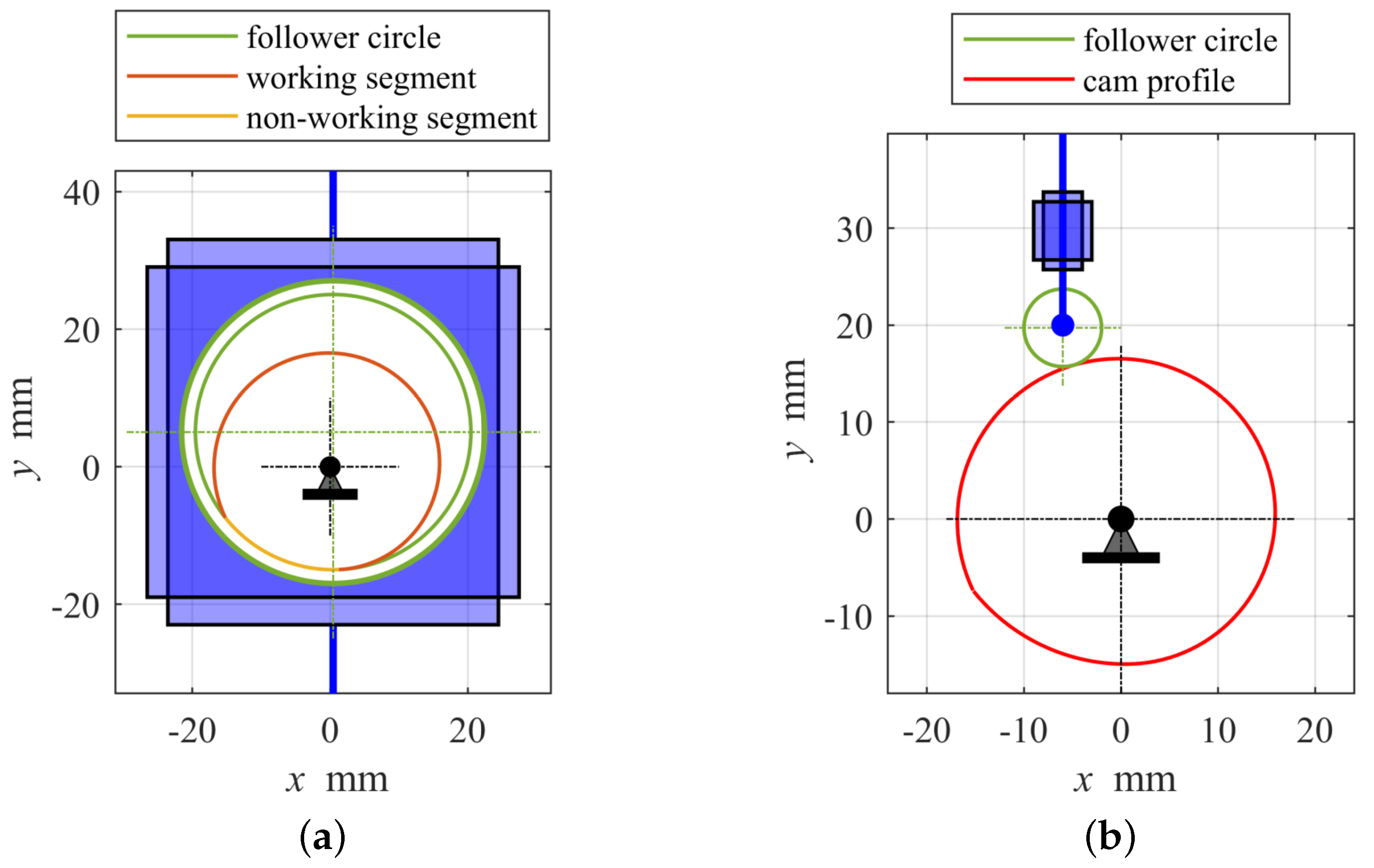
3.2. Design of Non-Working Segment Profile of Cam

The operation of the EMB is clamping to different clamping force or loosening, which is different from the common cam working process. This requires the cam to swing to a different angle rather than rotate continuously. Therefore, the cam profile in the EMB will not be used for a complete cycle. The design in this paper mainly focuses on the working segment profile. The working segment profile means that the profile can be tangent to the driven bearing in the normal working process. The profile not tangent to the driven bearing becomes the non-working segment. Determining the non-working segment is essentially a boundary constraint for the working segment. In order to enhance the strength of the camshaft as much as possible and not interfere with other parts, we selected the arc section with the same inner diameter of the driven bearing as the non-working segment. The initial position of cam rotation is the most easily interfered position. As shown in Figure 6, blue represents the driven bearing inner ring, and red represents the polar radius of the initial and final positions.

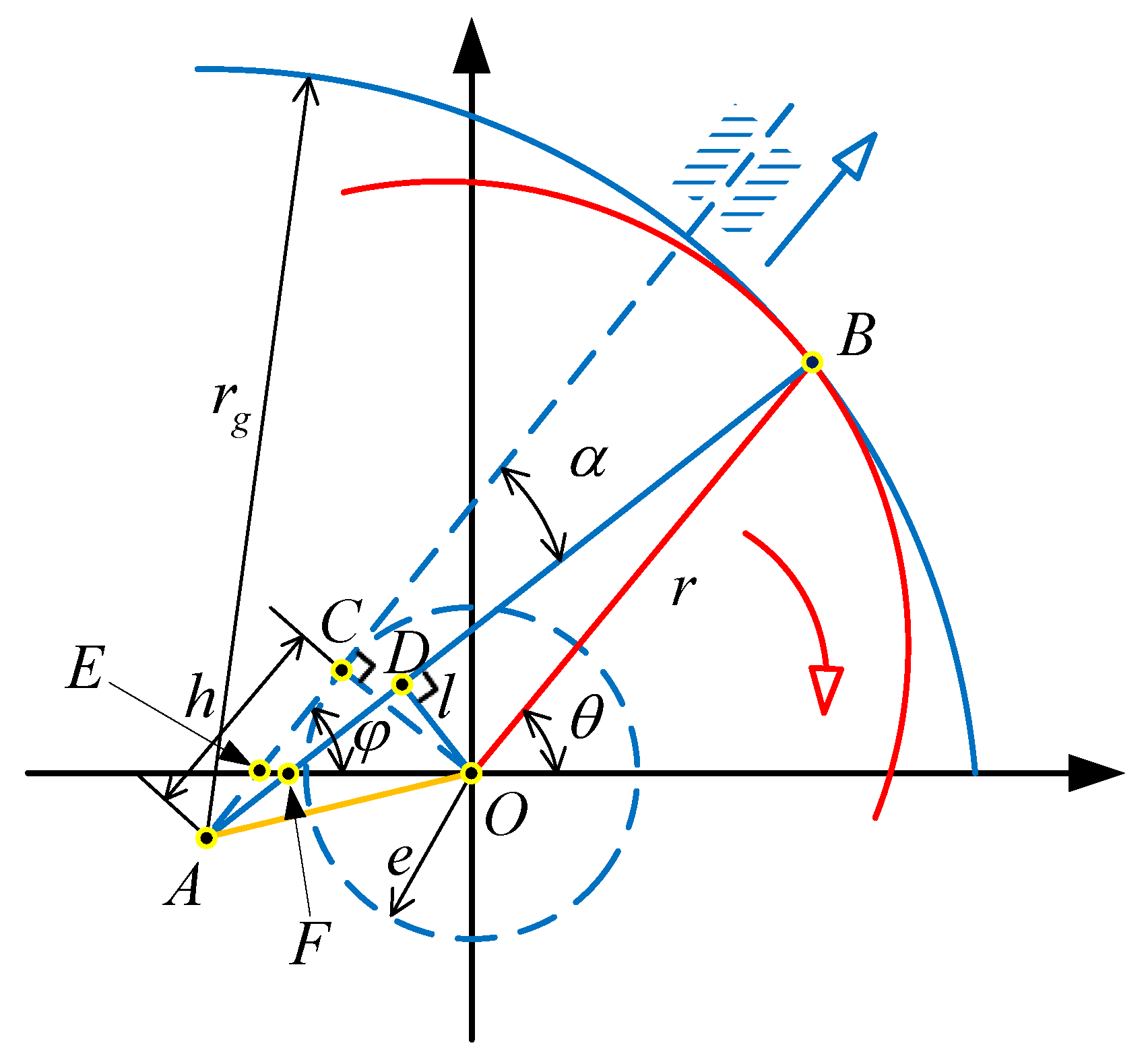
Let the initial contact position of the cam and driven inner ring be $B_{st}$, the radius from the contact point to the rotation center of the cam be $r_{st}$, the final contact position be $B_{end}$, and the radius to the rotation center be $r_{end}$. The design of the non-working segment shall ensure that it will not interfere when the cam moves. Therefore, in the initial position state, the end position with the largest radius is just on the driven circle.

Make the non-working segment profile tangent to the working segment profile at the initial position. Therefore,

$$tan\kappa =\frac{1}{r_{st}}{\left.\frac{dr}{d\theta }\right|}_{\begin{array}{c}r=r_{st}\\ \theta ={\theta }_0\end{array}}$$

(19)

The slope at the end of the initial position profile is

$${\left.\frac{dr}{d\theta }\right|}_{\begin{array}{c}r=r_{st}\\ \theta ={\theta }_0\end{array}}=r_{st}tan\kappa$$

(20)

Obviously, the initial tangent point should be on the left side of the straight line $OA$, and the rotation center O cannot be outside the roller. According to the geometric relationship, the initial position tangent angle should meet the following requirements:

$$0\le \kappa \le arccos\left(\frac{r_{st}}{2r_g}\right)$$

(21)

In addition, the initial profile angle ${\theta }_0$ and the total profile angle ${\theta }_a$ of the working segment need to be resolved. In $▵A{B}_{st}O$, using the cosine theorem:

$$\left|AO\right|=\sqrt{r_g^2+r_{st}^2-2r_g{r}_{st}cos\kappa }$$

(22)

Therefore, by using the cosine theorem in $▵A{B}_{st}O$ and $▵A{B}_{end}O$ twice, the total profile angle can be obtained as

$$\begin{array}{c}{\theta }_a=\angle B_{st}OA+\angle B_{end}OA=arccos\left(\frac{{\left|OA\right|}^2+r_{st}^2-r_g^2}{2\left|OA\right|r_{st}}\right)+arccos\left(\frac{{\left|OA\right|}^2+r_{end}^2-r_g^2}{2\left|OA\right|r_{end}}\right)\end{array}$$

(23)

Let $AH$ be the movement direction of the follower at the initial position, and make the vertical line $OH$ through O vertical with respect to $AH$, then $\left|OH\right|=e$ is the offset distance, then the initial profile angle is

$$\begin{array}{c}{\theta }_0=\frac{\pi }{2}-\angle HO{B}_{st}=\frac{\pi }{2}-\left(\angle AO{B}_{st}-\angle AOH\right)\\ =\frac{\pi }{2}-arccos\left(\frac{{\left|OA\right|}^2+r_{st}^2-r_g^2}{2\left|OA\right|r_{st}}\right)+arccos\left(\frac{e}{\left|OA\right|}\right)\end{array}$$

(24)

With the above information, the profile of the non-working segment of the cam is determined and can also be used to calculate the boundary conditions of the working segment.

3.3. Improved PSO Algorithm Design

According to the EMB function, the working segment profile of the cam can also be divided into two parts: (1) clearance elimination section; (2) clamping force control section. Then, the design requirements of the two sections can be summarized as follows:

(1) The rotation angle of the clearance elimination section shall be small to shorten the clearance elimination time;

(2) The transition from the clearance elimination section to the clamping force control section shall be free of impact;

(3) In the clamping force control section, the nonlinear relation between the rotation angle and the driving torque shall be weak, so as to facilitate the motor to control the clamping force;

(4) In the clamping force control section, the smaller the torque required to drive the cam is, the better, that is a large gain;

(5) The contact stress at any position of the clamping force control section shall meet the requirements without stress concentration;

(6) The cam mechanism meets the design total lift requirements;

(7) The profile shall be smooth enough, and the fluctuation of curvature radius shall be small;

(8) The profile will not interfere with distortion;

(9) Minimize the pressure angle during cam driving to improve transmission efficiency.

Based on the above design requirements, (1), (3), (4), (7), and (9) can be taken as the objectives of the profile design, and (2), (5), (6), and (8) are constraints. However, it is almost impossible to solve this functional extremum problem. 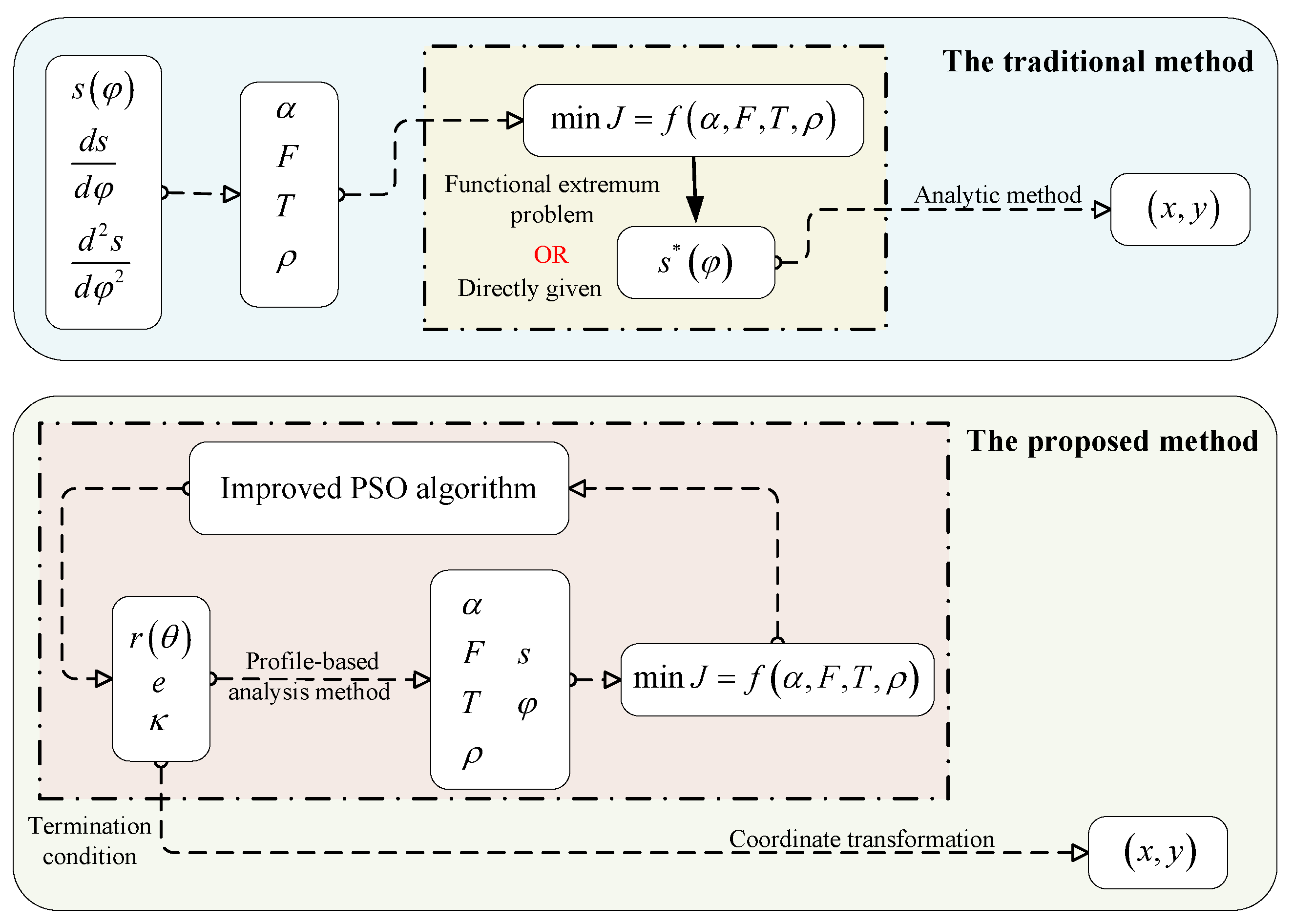Heuristic algorithms have been commonly used to solve such complex optimization problems in recent years, such as the genetic algorithm [35,36], the PSO algorithm [37,38], the ant colony algorithm [39], etc. Because some indicators of the objective function are composed of discrete key points, they do not have properties such as differentiability, continuity, etc. Therefore, many gradient-based optimization algorithms are difficult to apply. The PSO algorithm does not require the aforementioned properties and is relatively easy to program and implement. Therefore, in this study, the optimal solution is solved by the PSO algorithm. The process of the profile design is shown in Figure 7. A correction algorithm is proposed to accelerate the iterative convergence and improve the robustness of the algorithm, which is the main difference from the general PSO algorithm.

3.3.1. Design Variable

The purpose of the design variable selection is to give a complete description of the negative radius roller cam mechanism with a limited number of variables. Firstly, the coordinates describing the profile are selected in polar coordinates. The reason is that, in Section 2.3, the expression of the profile in polar coordinates can easily obtain various performance parameters of the cam.

Secondly, we used the spline curve to approximate the theoretical optimal profile. A sufficient number of key points are interpolated with the cubic spline curve, and the profile of any shape can be approximated with sufficient accuracy theoretically. Here, it is necessary to determine the number of key points N. Theoretically, the greater the number of key points is, the higher the accuracy of curve approximation will be, but the calculation cost will increase accordingly. More importantly, each key point cannot be completely independent. For a profile, the polar radius of adjacent key points often needs to be smooth and continuous, and the relations inside the particles will greatly affect the fitness of the particles. When the number of particles is too large, the internal freedom of the particles is too great, resulting in a very slow process of convergence to the optimal profile. To deal with this problem and improve the efficiency of the algorithm, in Section 3.3.4, this study will put forward a correction algorithm for the particle itself as an improvement to the PSO algorithm.

Third is the boundary condition selection and connection with the non-working segment. As coordinates, the cubic spline curve can be fully constrained by two boundary conditions. Meanwhile, the working segment and non-working segment of the cam need to be well connected. In Section 3.2, the non-working segment is designed, and they are tangentially connected at the initial position. At the final position, the working segment and the non-working segment need to be intersected. Because the cam is not allowed to cross the working segment into the non-working segment during normal operation, the tangential connection at the final position has little significance. Additionally, the distortion generated by the tangent will have an adverse impact on the motion characteristics of the final position. Therefore, the natural boundary condition is selected for the final position. In Section 3.2, the initial and total profile angles ${\theta }_0$ and ${\theta }_a$ of the working segment are determined, so the critical points of the cubic spline curve can be written as

$$\begin{array}{cc}\left({\theta }_0+\frac{{\theta }_a}{N}j,r_j\right)& j=0,1,\cdots ,N\end{array}-1$$

(25)

where, when $j=0$, $r_0=r_{st}$, the polar radius of the initial position is often given in advance in the axial strength design, so only the polar radius of the other $N-1$ critical points can be determined.

Finally is the offset design. The polar radius of $N-1$ critical points and the initial tangent angle $\kappa$ are able to uniquely determine the profile of the cam. However, the offset can also affect the characteristics of the cam mechanism.

Therefore, each particle can be expressed as

$$p_i=\left[\begin{array}{ccc}\begin{array}{ccc}{r}_1& \cdots & r_{N-1}\end{array}& \kappa & e\end{array}\right]$$

(26)

3.3.2. Objective Function

Firstly, the rotation angle of clearance elimination section is used as the evaluation measurement of the clearance elimination speed. The clearance elimination section cam angle ${\phi }_1={\left.\phi \right|}_{s=x_1}$ only needs to inversely solve the angle when the lift equals the clearance.

Secondly, we measured the linearity of driving torque to the rotation angle. The relation curve between the driving torque and rotation angle is the load characteristic of the EMB in front of the motor. Because the stiffness curve of the caliper device is not linear, it is not beneficial to the control of the EMB. It is expected to reduce the nonlinearity of the actuator after driving through the cam mechanism. When the derivative of the driving torque to the rotation angle approaches a certain constant, the driving torque linearity is better. To obtain a more-accurate linearity, the profile is interpolated to obtain more sample points, and then, the derivative variance is used as a measure, $\frac{{\displaystyle \sum _{v=1}^M}{\left({\left.\frac{dT}{d\phi }\right|}_v-{\displaystyle \sum _{u=1}^M}\left({\left.\frac{dT}{d\phi }\right|}_u\right)/M\right)}^2}{M}$.

Thirdly, the smaller the torque required for driving is, the better. Take the maximum value $max\left(T\right)$ of the driving torque as the measurement.

Fourthly, the profile shall be smooth enough. Therefore, the absolute value of the curvature radius difference of adjacent key points ${\displaystyle \sum _{j=1}^{N-1}}\left|{\rho }_j-{\rho }_{j-1}\right|$ shall be used as the measurement.

Finally, considering the transmission efficiency, it is measured by the pressure angle. The influence of the pressure angle on the transmission efficiency is represented on the cam by the lateral force generated on the follower when the cam is driven. It is more appropriate to measure the transmission efficiency with the maximum of the pressure angle tangent value $max\left(tan\left|\alpha \right|\right)$ (the absolute value because the pressure angle position is distinguished by the positive and negative pressure angles in Section 2). The transmission efficiency is close to 0 when the pressure angle is close to 90°, and $tan\alpha \to \infty$ at this time. Different weights are applied to the gap-elimination section and clamping section because the forces are less on the gap-elimination section.

To sum up, the weighted convex combination of the objective functions above can obtain a comprehensive objective function.

$$\begin{array}{c}Min:f=w_1{\theta }_1+w_2\frac{{\displaystyle \sum _{v=1}^M}{\left({\left.\frac{dT}{d\phi }\right|}_v-{\displaystyle \sum _{u=1}^M}\left({\left.\frac{dT}{d\phi }\right|}_u\right)/M\right)}^2}{M}+w_{3}max\left(T\right)\\ +w_4{\displaystyle \sum _{j=1}^{N-1}}\left|{\rho }_j-{\rho }_{j-1}\right|+w_{5}max\left({\left.tan\left|\alpha \right|\right|}_{s<x_1}\right)+w_{6}max\left({\left.tan\left|\alpha \right|\right|}_{x_1<s<x_1+x_2}\right)\end{array}$$

(27)

where $w_1,\cdots ,w_6$ are the goal weight factors.

3.3.3. Constraints

Because the cubic spline curve has a second-order continuous derivative, the whole working segment can naturally ensure continuity and no impact, so the design constraint (2) is satisfied, while other constraints can be written as

$$\left\{\begin{array}{c}{\sigma }_{Hmax}<{\left[\sigma \right]}_H\hfill \\ s\left({\theta }_0+{\theta }_a\right)=s_{max}\hfill \\ {\rho }_{max}\le r_g\hfill \end{array}\right.$$

(28)

where ${\sigma }_{Hmax}$ refers to the maximum contact stress when the cam is working, ${\left[\sigma \right]}_H$ refers to the allowable contact stress, $s\left({\theta }_0+{\theta }_a\right)$ refers to the lift at the end of the profile, and ${\rho }_{max}$ refers to the maximum curvature radius of the working segment profile.

The PSO algorithm cannot directly deal with the constraint, so we added the constraint into the target function in the form of a penalty function to synthesize the fitness value of the particle. The particles then move according to the fitness value to search for the optimal result.

$$fitness=f+g$$

(29)

where g is the penalty function, and it is represented by the piecewise function:

$$g=\left\{\begin{array}{cc}0& \mathrm{satisfy}\mathrm{constraints}\\ P_1+P_{2}err& \mathrm{otherwise}\end{array}\right.$$

(30)

where $err$ is the error not meeting the constraint $err\in \left\{{\left[\sigma \right]}_H-{\sigma }_{Hmax},\right.\left|s_{max}-s\left({\theta }_0+{\theta }_a\right)\right|,$ $\left.r_g-{\rho }_{max}\right\}$, and $P_1$ is the penalty factor, which is used to distinguish the constraint from the objective function. In general, it should be greater than the objective function $P_1>f$. There is basically no case where the constraint of the equation just meets the constraint, so this term is not required; $P_2$ is used to guide particles close to the direction meeting the constraint. For the constraint of the equation, two guiding factors can be used to approach from two directions of the equation.

3.3.4. Correction

There is too much freedom when using the key point to describe the cam profile, that is there is no constraint on the relationship between the key points. This leads to two problems: (1) some particles whose parameters break through the feasible domain will cause errors in the profile solution process and lead to program crash; (2) it is very inefficient to guide particles to the optimal profile by punishment. Therefore, the internal correction measures of particles are proposed in this study to limit the internal freedom of the particles to a certain extent. The particle is forced to move to the direction meeting the constraint, so as to improve the convergence speed of the algorithm. The particle correction specifically includes the following three aspects:

(1) Correction of particle parameter range: In Section 3.2, we give the range of the initial tangent angle as shown in Equation (21). For the offset distance, it is obvious that it shall meet $0<e<r_g$ to ensure that the initial tangent angle is not negative and the rotation center is within the driven circle. For the polar radius, it shall be ensured that the driven circle will not be interfered with in the horizontal direction and shall not be smaller than the polar radius of the critical point at the initial position, $\begin{array}{cc}{r}_{st}<r_j<r_g+e& j=1,\cdots ,N-1\end{array}$. When the parameters in the particles exceed the above limits, they are randomly assigned again within the feasible domain.

(2) Correction between adjacent key points: The correction between adjacent key points includes three parts: one is to ensure that the curvature radius of the profile is less than the curvature radius of the roller; the other is to ensure that the polar radius increases monotonously; the third is to slow down the change rate of the polar radius.

The condition that the profile of the roller cam mechanism with a negative radius is undistorted is that the radius of curvature is less than the radius of the roller. This condition can be guided by the penalty function with very low efficiency. Therefore, the correction of adjacent key points is significant.

As shown in Figure 8a, when the tangent angle and polar radius of the first key point are determined, to make the radius of curvature of the profile smaller than the radius of the roller, we can solve the critical case when the curvature is $r_g$. Solution $▵AO{B}_{st}$ can be obtained by using the cosine theorem:

$$\angle AO{B}_{st}=arccos\left(\frac{{\left|OA\right|}^2+r_{st}^2-r_g^2}{2\left|OA\right|r_{st}}\right)$$

(31)

where $\Delta \theta ={\theta }_a/\left(N-1\right)$ is the difference between the profile angles of two adjacent key points and $\left|OA\right|$ is shown in Equation (22).

Then, solve $▵AO{B}_{1max}$, because $\left|OA\right|<\left|A{B}_{1max}\right|=r_g$, so although the known $\angle AO{B}_{1max}=\angle AO{B}_{st}-\Delta \theta$ is not the angle between $OA$ and $A{B}_{1max}$, the triangle has only one solution, and the solution is

$$\left|O{B}_{1max}\right|=\left|OA\right|cos\angle AO{B}_{1max}+\sqrt{r_g^2+{\left|OA\right|}^2\left({cos}^2\angle AO{B}_{1max}-1\right)}$$

(32)

As shown in Figure 8b for subsequent key points, because the cubic spline curve must pass through the first two key points and the critical state of the curvature radius is when the three key points are on the circle with radius of $r_g$, the polar radius of the third key point shall be less than that case. The upper limit $\left|O{B}_{jmax}\right|$ of $r_j$ can be solved according to the geometrical relationship (see the Appendix A for details). Finally, the constraint relationship between adjacent key points can be comprehensively summarized as

$$\begin{array}{cc}{r}_j<\left|O{B}_{jmax}\right|& j=1,\cdots ,N-1\end{array}$$

(33)

Analyzing the clamping process of the EMB, it can be known that the lift of the cam always needs to be increased, so the polar radius of key point should also be monotonically increased.

$$\begin{array}{cc}{r}_{j-1}<r_j& j=1,\cdots ,N-1\end{array}$$

(34)

When the polar radius of a key point does not meet the range constrained by Equations (33) and (34), the key point is reinitialized with bias. Translate the subsequent key points as shown in Equation (35), preventing a chain reaction after reinitializing an abnormal key point and eliminate the advantageous features obtained through training.

$$\begin{array}{cc}{r}_{j+k}^{new}=r_{j+k}+\left(r_j^{new}-r_j\right)& k=1,\end{array}\cdots ,N-j-1$$

(35)

where $r_{j+k}^{new}$ represents the corrected polar radius of the key point.

The correction of curvature radius constraints is particularly important in the early stages of the algorithm. Because the initial motion amplitude and blindness of particles are large, which frequently appear, the profile cannot be solved. In the later stage of the algorithm, particle movement is more cautious and general. At this time, the constraint of the curvature radius should be relaxed to increase the degrees of freedom of particle activity, so that the particles can smoothly complete the movement and approach the optimal profile. Therefore, the correction process follows the general principle, with 100% triggering in the early stage and a gradual decrease in the probability of triggering in the later stage.

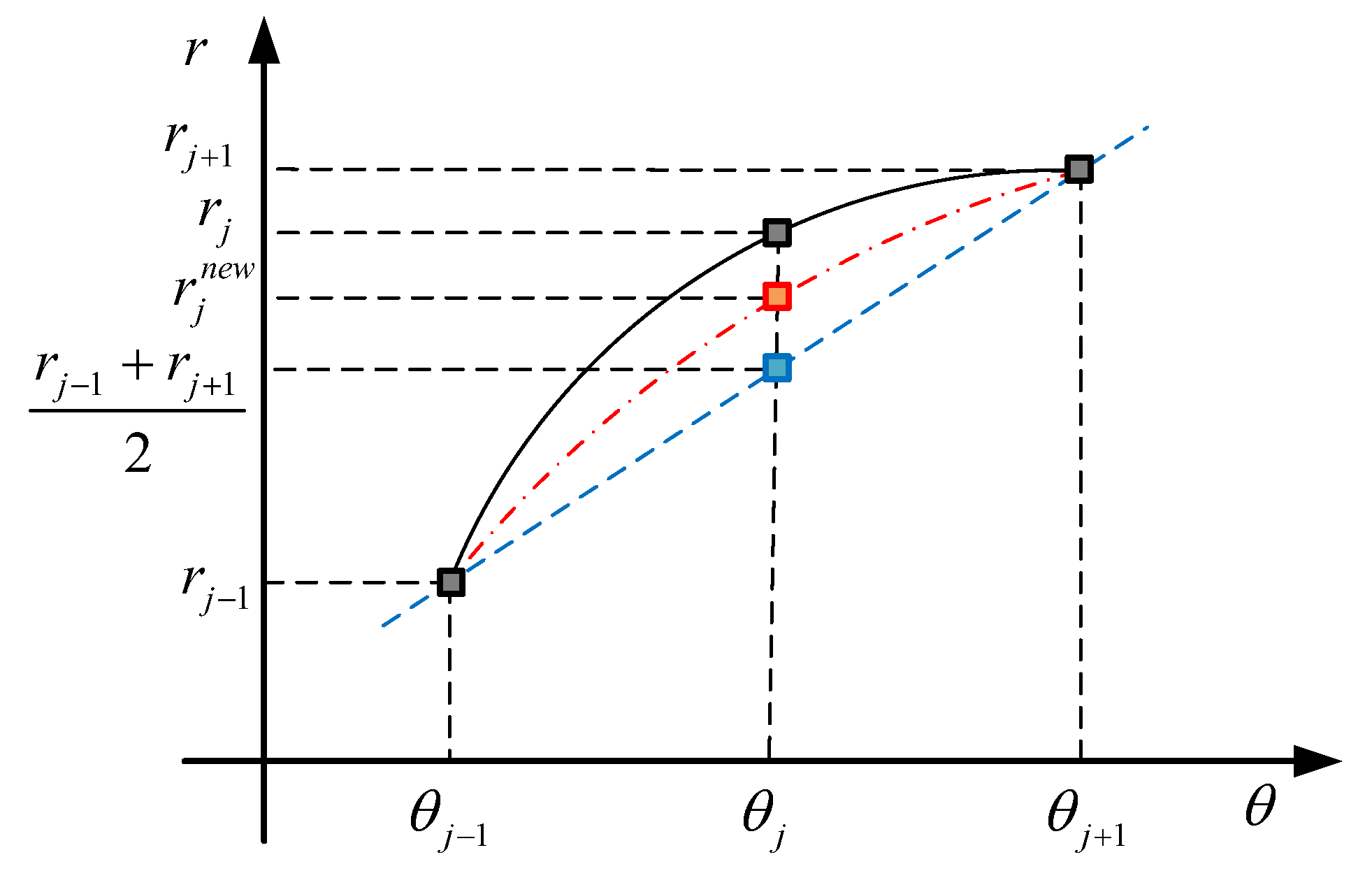
The correction of the rate of change in the polar radius of key points: The rate of change of the polar radius is related to the speed characteristics, and the greater the fluctuation of the rate of change of the polar radius, the greater the fluctuation of the speed characteristics of the cam is. Therefore, it is necessary to correct the change rate of the polar radius. As shown in Figure 9, the black solid line represents the polar radius of the three adjacent key points before correction, as shown by the blue dashed line. When the key points in the middle position are at the midpoint of the connecting line between the two key points, the change in polar radius is equal, and the rate of change is zero. Therefore, in order to reduce the rate of change of the polar radius, the corrected polar radius is located between the two and represented by a red dotted line. The new polar radius is represented as

$$\begin{array}{cc}{r}_j^{new}=\frac{1}{2}\left[r_j+\frac{1}{2}\left(r_{j-1}+r_{j+1}\right)\right]& j=1,\cdots ,N-2\end{array}$$

(36)

The correction of the rate of change of the polar radius is also based on probability. For the corrected expression of Equation (36), repeated iterations will result in $r_j\to \frac{1}{2}\left(r_{j-1}+r_{j+1}\right)$, and ultimately, all particles will become linearly increasing polar radii. Especially, excessive corrective intervention in the later stage of the algorithm will make it difficult for particles to autonomously search for the optimal profile, so the triggering probability of the algorithm is low and gradually decreases with the iterations.

(3) Correction of global key points: There is an important equality constraint in the constraint to ensure that the total lift of the cam meets the design requirements. However, the convergence speed of the approximation equation through particle movement is relatively slow, so the correction of global key points is used to correct the particle’s approximation towards the direction that meets the total lift requirements. Considering the significant correlation between the increase in the pole radius of the cam profile and the increase in the cam lift, the ratio of the actual total lift of the current particle to the designed total lift is used to perform a stretching transformation on the pole radius of the key point, as shown in Equation (37). Although the transformation cannot guarantee that the total lift meets the design requirements, it will make it closer. After multiple iterations, the equation constraints will be quickly approximated.

$$\begin{array}{cc}{r}_j^{new}=\left(r_j-r_{st}\right)\frac{s_{max}}{s\left({\theta }_0+{\theta }_a\right)}+r_{st}& j=1,\cdots ,N-1\end{array}$$

(37)

3.3.5. Location Update

The PSO algorithm [33] simulates bird predation. Each particle will determine the size and direction of its next motion based on the position of the globally optimal particle and the optimal position it has experienced. The expected motion speed of each particle:

$${\widehat{v}}_i^{k+1}=c_1{r}_{n1}\left(p_i-p_i^k\right)+c_2{r}_{n2}\left(g^k-p_i^k\right)$$

(38)

where ${\widehat{v}}_i^{k+1}$ is the expected motion velocity of the i-th particle for the $k+1$-st iteration; $c_1$ and $c_2$ are learning factors, $r_{n1}$ and $r_{n2}$ are random numbers, increasing search randomness; $p_i^k$ is the historical best position of the i-th particle; $g^k$ is the global optimal position for the k-th iteration.

At the same time, in order to avoid repeated oscillations in the initial stage of particle motion, each particle is affected by the inertia of the previous motion, and the actual motion speed is

$$v_i^{k+1}=\omega v_i^k+{\widehat{v}}_i^{k+1}$$

(39)

where $\omega$ is the inertia factor of motion; $v_i^k$ is the actual motion velocity of the i-th particle for the k-th iteration.

As the iteration progresses, both global and individual experiences are accumulated, and particle motion becomes more cautious. In order to obtain more-accurate solutions and gradually reduce the inertia factor, this article chose a linearly decreasing inertia factor:

$$\omega ={\omega }_{max}-\frac{i}{i_{max}}\left({\omega }_{max}-{\omega }_{min}\right)$$

(40)

where ${\omega }_{max}$ and ${\omega }_{min}$ are the upper and lower bounds of the inertia factor, i is the current number of iterations, and $i_{max}$ is the maximum number of iterations.

Update the particle position after obtaining the actual motion speed:

$$p_i^{k+1}=p_i^k+v_i^{k+1}$$

(41)

During the iteration process, the global optimal position and corresponding fitness are recorded each time. When the set number of iterations is reached, the iteration exits and the optimal particle is extracted to obtain the profile of the cam.

4. Discussion

4.1. PSO Parameter Discussion

The PSO algorithm has many parameters, and different parameter settings can have an impact on the iterative process and results of the algorithm. Based on the entire PSO algorithm design process, these parameters can be divided into four groups:

• Goal weight factors;
• Penalty coefficients;
• Correction probability coefficients;
• Particle parameters.

Goal weight factors are the compromise on design goals that cannot be achieved simultaneously. These parameters are $w_1,\cdots ,w_6$, as shown in Equation (27). The setting of these parameters mainly depends on the designer’s description of the expected goals. When setting specific values, it is usually necessary to consider the differences in the dimensions and range of variation of different goals. They are generally independent of the convergence of the iteration. The adjustment of goal weights usually does not have a direct impact on whether the algorithm falls into local optimization problems, but unreasonable parameters can cause the results to deviate from expectations. In this case, manual adjustment is required, which is usually improved through multiple debugging.

The penalty coefficients mainly act on particles that do not meet the constraints. The penalty coefficient $P_1$ shown in Equation (30) can reflect the priority of constraints by taking different values for different constraints. The penalty coefficient $P_2$ is an evaluation gradient constructed for particles that do not meet the constraint, which can guide particles to meet the constraint, to a certain extent. However, this guidance effect is weak. If initialized randomly, most particles cannot meet the constraints, and the convergence process is very slow.

The correction probability is proposed in the correction algorithm. The function of correction algorithms is to make particles satisfy constraints and make some of their targets superior. These operations are relatively general and one-sided and cannot be continuously applied in every iteration process, otherwise the final result will also become one-sided. The probability of triggering a correction usually increases in the early stages of the iteration, but in the later stages, it needs to be reduced or even completely closed. When the correction trigger frequency is too high, the algorithm usually converges quickly; however, particle diversity is limited, and the likelihood of falling into local optima increases. On the contrary, the convergence process will become very slow.

Because the objective function is too complex, similar to most heuristic algorithms, the results obtained by PSO are difficult to prove to be globally optimal. However, as long as the expected design goals are met, even if it is only a local optimum, it does not affect its value in practical applications.

The particle parameters are traditional parameters of the PSO algorithm, including the number of particles, number of iterations, coefficient of motion, etc. Because these parameters are not directly related to the problem requiring optimization, some scholars have conducted research on the selection of these parameters, and we refer to their conclusions [40].

4.2. Analysis of Improved PSO Algorithm Results

4.2.1. Iterative Process Analysis

Figure 10a shows the fitness of the optimal particles generated by each iteration of the particle swarm optimization in the iteration process. Due to the correction algorithms, the optimal particles generated in the first iteration already meet the inequality constraint requirements. Subsequent iterations involve fine-tuning optimization and approximating the equality constraints. Figure 10b shows the pole radius of the key points for the optimal particle in each iteration. At the beginning, optimal particles change significantly, while the later adjustment is very small. The initial tangent angle and offset distance of particles exhibit similar changes, with minor changes after approximately 100 iterations. In addition, comparing Figure 10c,d, the offset distance converges approximately 29 iterations faster than the initial tangent angle, which may be related to the fact that the offset distance is independent of the cam shape.

4.2.2. Analysis of Convergence Situation

The state of the particle swarm at the end of the iteration is shown in Figure 11. In Figure 11a, it can be seen that the key point pole radii of other particles are mostly near the optimal particle, which means the algorithm has converged. The coincidence degree of the first few key points is higher compared to the last few key points. The reason for this phenomenon is that the correction between adjacent key points results in superposing a greater degree of freedom for later key points. Observing Figure 11b,c, it is found that the offset distance and initial tangent angle of the vast majority of particles have converged to the vicinity of the optimal particle. Thus, 86% of other particles’ offset distances have less than 0.01 mm removed from the optimal particle, so that 85% the initial tangents have less than 0.01 rad removed from the optima.Compared with the optimal particle, the offset distance of other particles is basically symmetrical, while the initial tangent angle is mainly distributed on the right side, which is related to the initial distribution.

4.2.3. Analysis of Design Results

We calculated the optimal particle parameters at the end of the iteration to obtain the cam profile. Its shape is drawn as Figure 1a.

The calculated curvature radius of the profile is shown in Figure 12a. If the curvature radius is smaller than the driven roller radius, the cam follower’s motion will not have distortion. Besides, the curvature radius is continuous and relatively smooth. The contact stress on the cam profile during the EMB clamping process is shown in Figure 12b, and the results showed that it can meet the contact stress requirements. Other design goals and constraints will be analyzed in Section 4.3.2.

4.3. Profile-Based Analysis Method Validation

4.3.1. Verification of Speed Characteristics and Force Transmission Characteristics

The profile-based analysis method proposed in this article directly derives the torque T, clamping force $F_{ca}$, lift s, and rotation angle $\phi$ during the working process of the cam from the profile. The relationship between the lift and rotation angles is obtained through geometric relationships, while that of the torque and clamping force is through the force relationship. According to Equations (12) and (14), they have the relationship:

$$T=F_{ca}\frac{l}{cos\alpha }$$

(42)

The deformation of Equation (2) based on the equality of instantaneous power:

$$T=F_{ca}\frac{ds}{d\phi }$$

(43)

Therefore, it can be obtained that

$$\frac{T}{F_{ca}}=\frac{ds}{d\phi }=\frac{l}{cos\alpha }$$

(44)

By using numerical differentiation and interpolation methods, the values of both expressions can be calculated as shown in Figure 13a, and the error between them can be calculated as shown in Figure 13b. The error and the actual value are not on the same order, and the error is related to the number of sampling points in the numerical calculation. From this, it can be verified that the cam-profile-based analysis method is logically self-consistent.

4.3.2. ADAMS Simulation Model Comparison

To further validate the designed profile, we imported the designed cam EMB into ADAMS for simulation. As shown in Figure 14a, the red part is the camshaft and the driven bearing on the follower in blue was simplified. The green part is the caliper, and we fixed it to the ground. The camshaft and caliper are connected by a rotating pair, while the driven bracket and caliper are connected by a moving pair.

A nonlinear spring is set between the driven bracket and the caliper to simulate the caliper defined in Section 3.1, as shown in Figure 14b. Input a constant speed rotation of 1°/s on the camshaft to achieve the EMB action. The contact between the cam and the driven bracket is the most-core relationship in the cam simulation process. This article selected the impact contact model, and the parameters are defined as the contact parameters between steel and steel, as shown in Figure 14c.

Figure 15 compares the four physical quantities of the cam including the lift, pressure angle, driving torque, and clamping force. Because the contact force is defined by two objects invading each other, as shown in Figure 15a, the lift of the cam is relatively small. Especially in the clamping section, where the contact force between the cam and the follower is greater, this results in greater lift error. When the clamping force is not generated, there is a large amount of shaking in the lift error, which is caused by insufficient clamping force to limit the follower. The pressure angle in ADAMS is calculated by the ratio of the transverse component and the longitudinal component of the contact force. Because the clamping force is almost zero during clearance elimination, the pressure angle cannot be calculated. When entering the clamping section, the calculated pressure angle is basically accurate. As shown in Figure 15c, the driving torque has good linearity according to the design objective. As shown in Figure 15c,d, due to the presence of invasion deformation, the driving torque and actual clamping force in ADAMS are relatively small. Especially when the clamping force is large, the stiffness of the caliper is very high, and even small invading deformation is reflected in the force. Therefore, there should be a certain margin in cam design to compensate for this part of deformation.

4.4. Discussion on the Cam EMB

The ball screw is now the most-commonly used mechanism on the EMB, and its structure is shown in Figure 16. The rolling balls between the screw and nut convert the relative sliding into rolling. The design parameters of the screw include the lead, the nominal diameter, the length of the nut, etc. The only parameter related to the transmission characteristics of the screw is the lead. The lead refers to the distance that the screw rotates one turn and the nut moves forward. Other parameters mainly affect the volume and bearing capacity. Due to the high processing requirements for ball screws such as ball raceways, these parameters are usually serialized.

To compare the cam EMB with other mechanisms of EMBs, we conducted a comparison under the same assumptions. Compare the cam mechanism designed in this article with a screw with the same maximum rotation angle to achieve the same displacement. The lead of the screw compared is

$$p=\frac{s_{max}}{{\phi }_{max}}2\pi$$

(45)

By incorporating the parameters obtained from the optimized design, the lead of the compared screw should be 2.40 mm, In fact, if it is necessary to withstand a load of 50 kN, the lead of the ball screw usually needs to be above 4 mm, and the structural volume is larger. To control the variables for comparison, we assumed the existence of the ideal ball screw mentioned above, and the torque required for the ball screw at the position with the largest load is

$$T_{max}=\frac{F_{camax}p}{2\pi }$$

(46)

The calculated torque required to drive the screw is 19.06 N·m, while from Figure 15c, it can be seen that the optimized cam mechanism only requires a torque of 7.72 N·m. When both the camshaft and the ball screw rotate at the same speed and their clamping force can reach the maximum load, the motor power of the cam is only 40.52% of the motor power of the screw, which is expected to match a smaller power motor and further reduce the volume of the EMB. In fact, both the cam mechanism and the screw mechanism are transmission mechanisms that do not amplify or reduce power without considering efficiency. The reason why the cam mechanism can match smaller motors is that the EMB caliper device has strong nonlinearity, and the optimized design of the cam can effectively modify this nonlinear load characteristic and fully utilize the motor power.

In terms of clearance elimination, the cam needs to rotate at an angle of 1.72 rad to eliminate the clearance, while the ball screw needs 2.62 rad. When both the camshaft and the lead screw rotate at the same speed, the time required to eliminate the same brake clearance for the cam EMB is only 65.65% of the ball screw EMB.

However, compared to the screw mechanism, the disadvantage of the cam mechanism is that it cannot continuously generate movement, so a separate clearance adjustment device [29] is needed to achieve clearance adjustment. In addition, the factors of friction and efficiency were less considered in the above design and analysis process, while in fact, they play an important role in the transmission process. Therefore, further experimental testing or other methods are needed to obtain their characteristics in the future and then redesign the camshaft based on these characteristics. Fortunately, the redesigned camshaft has little impact on the overall dimensions, so it is feasible in reality.

5. Conclusions

This article proposes a novel type of EMB based on the native radius roller cam mechanism. To achieve the ideal characteristics of the EMB, we proposed a design method for the core component, the cam mechanism. Firstly, we propose a new analysis method for negative radius roller cams, starting from the profile. Secondly, we used the improved PSO algorithm to solve the complex multi-objective optimization problem, which is essentially a nonlinear functional extreme value problem. Then, the effectiveness of the method was demonstrated through algorithm self-validation and comparison with ADAMS simulation. Finally, we discussed the advantage of the cam EMB compared with the screw mechanism.

In the future, we will design and process a negative radius roller cam mechanism EMB and matching gap automatic adjustment devices. Besides, the native radius roller cam mechanism can not only be used in EMBs, but also in potential applications such as machine tool fixtures that require the control of the clamping force.

In addition, the profile-based analysis method has certain practical value for analyzing unknown cams, cams with machining errors, or cams with wear by only detecting the profile. It can quickly establish a cam mechanism dynamics model for simulation and other purposes.

However, the process of PSO involves a large amount of randomness, and different initial values also have a certain impact on the algorithm’s results, resulting in inconsistent final iteration results, and the optimality of the solution cannot be theoretically proven. However, the results are sufficient to prove that the application performance of cam mechanisms on EMBs can be improved by designing different profiles.

6. Patents

We have submitted two Chinese patents for this new type of EMB [28,29] (Patent applying number: No. 202310700946.8 and No. 202310704533.7).

References

1. Peng, H.; Chen, X. Active Safety Control of X-by-Wire Electric Vehicles: A Survey. Sae Int. J. Veh. Dyn. Stab. NVH 2022, 6, 115–133. [Google Scholar] [CrossRef]
2. Zhang, L.; Zhang, Z.; Wang, Z.; Deng, J.; Dorrell, D.G. Chassis Coordinated Control for Full X-by-Wire Vehicles—A Review. Chin. J. Mech. Eng. 2021, 34, 555. [Google Scholar] [CrossRef]
3. Maron, C.; Dieckmann, T.; Hauck, S.; Prinzler, H. Electromechanical Brake System: Actuator Control Development System. In Proceedings of the SAE International Congress & Exposition, Wichita, Kansans, 30 September–2 October 1997; SAE International Congress & Exposition: Greenville, SC, USA, 1997. [Google Scholar]
4. Gong, X.; Ge, W.; Yan, J.; Zhang, Y.; Gongye, X. Review on the Development, Control Method and Application Prospect of Brake-by-Wire Actuator. Actuators 2020, 9, 15. [Google Scholar] [CrossRef]
5. Heydrich, M.; Ivanov, V.; Bertagna, A.; Rossi, A.; Mazzoni, M.; Bücner, F. Hardware-in-the-Loop Testing of a Hybrid Brake-by-Wire System for Electric Vehicles. SAE Int. J. Veh. Dyn. Stab. NVH 2022, 6, 477–487. [Google Scholar] [CrossRef]
6. Liu, Y.; Pei, X.; Guo, X. Redundancy Control of Anti-lock Braking System Based on Electro-hydraulic Braking System. SAE Int. J. Veh. Dyn. Stab. NVH 2023, 7, 53–67. [Google Scholar] [CrossRef]
7. Li, T.; Shi, Q.; Lei, Z.; He, L.; Liu, B. Research on Mechanism and Key Technology of Intelligent Vehicles Brake By Wire system. In Proceedings of the 2019 3rd Conference on Vehicle Control and Intelligence (CVCI), Nanjing, China, 28–30 October 2019; pp. 1–8. [Google Scholar]
8. Yu, L.; Liu, X.; Xie, Z.; Chen, Y. Review of Brake-By-Wire System Used in Modern Passenger Car. In International Design Engineering Technical Conferences and Computers and Information in Engineering Conference; American Society of Mechanical Engineers: New York, NY, USA, 2016. [Google Scholar]
9. Liu, Y.; Chen, X. Structural Analysis and Design of Actuator Mechanisms for Electro-Mechanical Brake (EMB). In Proceedings of the International Conference on Chinese Institutions and Machine Science (CCMMS 2010), Shanghai, China, 21–25 July 2010; pp. 61–63. [Google Scholar]
10. Schumann, F. Electromacanic Wheel Brake Device. US Patent 6 305 508 B1, 25 December 2001. [Google Scholar]
11. Chen, Q.; Lv, Z.; Tong, H.; Xiong, Z. Clamping Force Control Strategy of Electro-Mechanical Brake System Using VUF-PID Controller. Actuators 2023, 12, 272. [Google Scholar] [CrossRef]
12. Xiao, F.; Gong, X.; Lu, Z.; Qian, L.; Zhang, Y.; Wang, L. Design and Control of New Brake-by-Wire Actuator for Vehicle Based on Linear Motor and Lever Mechanism. IEEE Access 2021, 9, 95832–95842. [Google Scholar] [CrossRef]
13. Tonoli, A.; Voyat, J.; Fracassi, G. Electromechanical Actuating Device for a Wheel Brake System of a Motor Vehicle and a Brake System Equipped with Such an Actuating Device. European Patent 1 798 123 A1, 24 May 2005. [Google Scholar]
14. Putz, M. Electrically Actuated Friction Brake. European Patent 2 971 840 B1, 30 April 2014. [Google Scholar]
15. Carra, S.; Garziera, R.; Pellegrini, M. Synthesis of cams with negative radius follower and evaluation of the pressure angle. Mech. Mach. Theory 2004, 39, 1017–1032. [Google Scholar] [CrossRef]
16. Hejma, P.; Svoboda, M.; Kampo, J.; Soukup, J. Analytic Analysis of a Cam Mechanism. Procedia Eng. 2017, 177, 3–10. [Google Scholar] [CrossRef]
17. Flocker, F.W. A Versatile Acceleration-Based Cam Profile for Single-Dwell Applications Requiring Cam-Follower Clearance During Dwell. J. Mech. Des. 2012, 134, 987–997. [Google Scholar] [CrossRef]
18. Gao, F.; Liu, Y.; Liao, W.H. Cam Profile Generation for Cam-Spring Mechanism With Desired Torque. J. Mech. Robot.-Trans. Same 2018, 10, 7. [Google Scholar] [CrossRef]
19. Hoang, P.H.; Ngoc, L.Q. Program for Designing Planar Cam Mechanisms. In Proceedings of the 2018 4th International Conference on Green Technology and Sustainable Development (Gtsd), Chi Minh City, Vietnam, 23–24 November 2018; p. 6. [Google Scholar]
20. Yao, Y.A.; Zhang, C.; Yan, H.S. Motion control of cam mechanisms. Mech. Mach. Theory 2000, 35, 15. [Google Scholar] [CrossRef]
21. Demeulenaere, B.; Berkof, R.S. Improving machine drive dynamics: A structured design approach toward balancing. J. Mech. Des. 2008, 130, 082302. [Google Scholar] [CrossRef]
22. Zhu, G.; Wang, Y.; Zhu, G.N.; Weng, M.; Liu, J.; Zhou, J.; Lu, B. Parameter Optimization of Large-Size High-Speed Cam-Linkage Mechanism for Kinematic Performance. Actuators 2023, 12, 2. [Google Scholar] [CrossRef]
23. Qu, X.; Cao, D.; Qu, R.; Zhang, G.; Zhang, S. A Novel Design of Torsion Spring-Connected Nonlinear Stiffness Actuator Based on Cam Mechanism. J. Mech. Des. 2022, 144, 083303. [Google Scholar] [CrossRef]
24. Lopez-Martinez, J.; Garcia-Vallejo, D.; Manuel Arrabal-Campos, F.; Manuel Garcia-Manrique, J. Design of Three New Cam-Based Constant-Force Mechanisms. J. Mech. Des. 2018, 140, 082302. [Google Scholar] [CrossRef]
25. Lin, R.F.; Chang, Y. Optimization Design of Disc Cam Mechanisms with an Offset Translating Negative Radius Roller Follower. Appl. Mech. Mater. 2012, 184–185, 774–779. [Google Scholar] [CrossRef]
26. Lin, R.F.; Chang, Y. Mechanical Analysis of Disc Cam Mechanisms with Negative Radius Roller Translating Follower. Appl. Mech. Mater. 2012, 184–185, 301–306. [Google Scholar] [CrossRef]
27. Hidalgo-Martínez, M.; Sanmiguel-Rojas, E.; Burgos, M.A. Design of cams with negative radius follower using Bézier curves. Mech. Mach. Theory 2014, 82, 87–96. [Google Scholar] [CrossRef]
28. Yan, M.; Yan, Z.; Chen, X. Cam Electro-Mechanical Brake and Vehicle. CN 202310704533.7, 2023. [Google Scholar]
29. Yan, Z.; Yan, M.; Chen, X. Electro-Mechanical Brake with Clearance Adjustment Based on One-Way Self-Locking Mechanism. CN Patent 202310700946.8, 4 March 2023. [Google Scholar]
30. Chang, Y.; Li, Y.P. The Auxiliary Angle Method for Deriving the Pressure-Angle Expressions of Cam Mechanisms. Adv. Mater. Res. 2010, 102–104, 267–271. [Google Scholar] [CrossRef]
31. Deng, Z.; Yu, H.; Wang, Z. Mechanisms and Machine Theory, 3rd ed.; Higher Education Press: Beijing, China, 2015. [Google Scholar]
32. Fu, Y.F.; Hu, X.H.; Wang, W.R.; Ge, Z. Simulation and Experimental Study of a New Electromechanical Brake with Automatic Wear Adjustment Function. Int. J. Automot. Technol. 2020, 21, 227–238. [Google Scholar] [CrossRef]
33. Kwon, S.; Lee, S.; Lee, J.; Kum, D. Accurate State Estimation for Electro-Mechanical Brake Systems. J. Electr. Eng. Technol. 2019, 14, 889–896. [Google Scholar] [CrossRef]
34. Xu, Z.; Gerada, C. Enhanced Force Estimation for Electromechanical Brake Actuators in Transportation Vehicles. IEEE Trans. Power Electron. 2021, 36, 14329–14339. [Google Scholar] [CrossRef]
35. Hamza, F.; Abderazek, H.; Lakhdar, S.; Ferhat, D.; Yıldız, A.R. Optimum design of cam-roller follower mechanism using a new evolutionary algorithm. Int. J. Adv. Manuf. Technol. 2018, 99, 1267–1282. [Google Scholar] [CrossRef]
36. Lampinen, J. Cam shape optimisation by genetic algorithm. Comput.-Aided Des. 2003, 35, 727–737. [Google Scholar] [CrossRef]
37. Najjari, M.; Guilbault, R. Formula derived from particle swarm optimization (PSO) for optimum design of cylindrical roller profile under EHL regime. Mech. Mach. Theory 2015, 90, 162–174. [Google Scholar] [CrossRef]
38. Al Kouzbary, M.; Al Kouzbary, H.; Liu, J.; Khamis, T.; Al-Hashimi, Z.; Shasmin, H.N.; Arifin, N.; Abu Osman, N.A. Robotic Knee Prosthesis with Cycloidal Gear and Four-Bar Mechanism Optimized Using Particle Swarm Algorithm. Actuators 2022, 11, 253. [Google Scholar] [CrossRef]
39. Li, Z.; Chang, X.; Lou, Y. Optimization Design of Distribution Cam Mechanism in Internal Combustion Engine Based on Improved Ant Colony Algorithms. J. Mech. Strength 2005, 27, 146–150. [Google Scholar] [CrossRef]
40. Juang, Y.T.; Tung, S.L.; Chiu, H.C. Adaptive fuzzy particle swarm optimization for global optimization of multimodal functions. Inf. Sci. 2011, 181, 4539–4549. [Google Scholar] [CrossRef]
Figure 1. Comparison between negative radius roller cam mechanism and positive radius roller cam mechanism. (a) Negative radius roller cam mechanism; (b) positive radius roller cam mechanism.
Actuators 12 00329 g001
Figure 2. Negative radius roller cam mechanism electronic mechanical brake (EMB). (a) Overall assembly rendering; (b) schematic diagram of the principle, where 1—driven bracket; 2—driven bearing; 3—camshaft; 4—friction plate; 5—caliper housing; 6—caliper bracket; 7—brake disc.
Actuators 12 00329 g002
Figure 3. The block diagram of the cam design method proposed in this article and traditional thinking.
Actuators 12 00329 g003
Figure 4. Schematic diagram of the negative radius roller cam mechanism based on the profile-based analysis method.
Actuators 12 00329 g004
Figure 5. Schematic diagram of the relationship between the rotation angle and profile angle. The figure displays a pointed cam, with the tangent point of the negative radius roller cam corresponding to the pointed point of the pointed cam mechanism.
Actuators 12 00329 g005
Figure 6. Design of non-working segment profile.
Actuators 12 00329 g006
Figure 7. Improved particle swarm optimization (PSO) algorithm flow chart.
Actuators 12 00329 g007
Figure 8. Schematic diagram of curvature radius correction. (a) Correction for the second key point; (b) correction for the j + 1 -th key point.
Actuators 12 00329 g008
Figure 9. Schematic diagram for correcting the polar radius of key points.
Actuators 12 00329 g009
Figure 10. Improve the parameter changes of globally optimal particles during the iteration process of the PSO algorithm. (a) Fitness; (b) key point pole radii; (c) initial tangent angle; (d) offset distance.
Actuators 12 00329 g010
Figure 11. The parameter situation of the optimal particle and other particles at the end of the iteration. (a) Key point pole radii; (b) offset distance; (c) initial tangent angle.
Actuators 12 00329 g011
Figure 12. The curvature radius and contact stress on the cam profile. (a) Curvature radius; (b) contact stress.
Actuators 12 00329 g012
Figure 13. Verification of motion characteristics and force transmission characteristics. (a) Curve obtained from two dimensions; (b) curve error.
Actuators 12 00329 g013
Figure 14. ADAMS model and simulation settings. (a) Schematic diagram of the ADAMS model; (b) caliper stiffness model. Describe using spline curve method, with the horizontal axis representing the lift of the driven bracket and the vertical axis representing the clamping force; (c) contact parameter setting between cam and driven bracket.
Actuators 12 00329 g014
Figure 15. Comparison of the results between the profile-based analysis method and the ADAMS model. (a) The cam lift and its error; (b) the pressure angle and its error; (c) the drive torque and its error; (d) the clamping force and its error.
Actuators 12 00329 g015
Figure 16. Ball screw EMB. In the figure, 1—nut, 2—ball, 3—screw, and 4—thrust bearing. When the screw rotates, the nut moves forward, and the screw transmits the force to the caliper through a thrust bearing. p is the lead of the ball screw; D is the nominal diameter; S a is the length of the nut.
Actuators 12 00329 g016
Disclaimer/Publisher’s Note: The statements, opinions and data contained in all publications are solely those of the individual author(s) and contributor(s) and not of MDPI and/or the editor(s). MDPI and/or the editor(s) disclaim responsibility for any injury to people or property resulting from any ideas, methods, instructions or products referred to in the content.