A Real-Time Path Planning Algorithm Based on the Markov Decision Process in a Dynamic Environment for Wheeled Mobile Robots

Abstract

A real-time path planning algorithm based on the Markov decision process (MDP) is proposed in this paper. This algorithm can be used in dynamic environments to guide the wheeled mobile robot to the goal. Two phases (the utility update phase and the policy update phase) constitute the path planning of the entire system. In the utility update phase, the utility value is updated based on information from the observable environment. Obstacles and walls reduce the utility value, pushing agents away from these impassable areas. The utility value of the goal is constant and is always only the largest. In the policy update, a series of policies can be obtained by the strategy of maximizing its long-term total reward, and the series will eventually form a path towards the goal, regardless of where the agent is located. The simulations and experiments show that it takes longer to find the first path in the beginning due to the large changes of utility value, but once the path is planned, it requires a small amount of time cost to respond to the environmental changes. Therefore, the proposed path planning algorithm has an advantage in dynamic environments where obstacles move in unpredictable ways.

1. Introduction

Path planning plays an important role in industrial applications, including automated guided vehicles, unmanned aerial vehicles, and robotic arms. Although the constraints will vary by the agent, the aim of path planning is to provide the agent with a path from the current or specified location to the destination. In various methods used in the past, the A* search algorithm is the well-known, heuristic and best-first search algorithm for path planning.

The A* algorithm has the property of completeness (that is, the path can always be found out if there exist some paths from the starting point to the goal point). The evaluation function of this algorithm is formed by adding the current cost and the estimated cost. The estimated cost is a heuristic function used to estimate the cost from the current point to the goal point. If the cost does not exceed the actual cost, the solution has the property of optimality. If this cost is always equal to the actual cost, it has the least search space. If no future estimates are made, this algorithm will be equivalent to the Dijkstra algorithm and is equally complete and optimal. In continuous space, the heuristic function commonly used for path planning uses Euclidean distance to ensure that the path is optimal. Since the A* algorithm gradually explores outward from one or a few points, the step size of the exploration cannot be infinitely small. In other words, the map must be discretized, or at least a limited number of nodes must be established in a specific way. Discretization into a grid is one of the most classic methods. Its method is to divide the map into many blocks at equal distances and to store them as an array, so each element of the array corresponds to an actual space. The advantage of this method is that the segmentation method and the content of the map are independent so that it can be applied to most occasions. However, the scope of each exploration only covers the adjacent nodes of the current node, which limits the direction of the path and means that the planned path may not meet the actual optimality. In addition, the resolution of the grid method is a parameter that requires designers to weigh cost and performance, and the area bordered by obstacles is in a mixed state, that is, there are some passable objects and some obstacles in the same area, so that the robot passing through this area must be aware of collision issues. Using road endpoints or corners of object shapes as nodes is also a feasible design method. This design can greatly reduce the search space and improve the problem of limited path movement. However, the location and connection of nodes will depend on the map content and need to be matched with other algorithms. The path quality is greatly affected by the way nodes are established.

Many path planning studies are based on the A* algorithm or improve it for its shortcomings [1,2]. The heuristic function of the A* algorithm is modified in [1] as f(n) = g(n) + αh(n), where α is dynamically adjusted by the Q-learning algorithm. This adjustment mechanism enables the method to adjust the path of the bureau road, thereby achieving real-time obstacle avoidance. In [2], a path post-processing smoothing mechanism is proposed, using the Bezier curve to replace part of the path to solve the problem of path discontinuity at turning.

Since the A* search algorithm requires a large computational cost in a high-dimensional space, a Rapidly-exploring random tree (RRT) based on random search is also a common method in path planning [3]. Instead of choosing the next node from the adjacent node of the current node, the distances between the next and current nodes are random. Hence, RRT has special advantages in efficiency and is suitable for high-dimensional fields, such as tandem robotic arms. However, the RRT algorithm is only probabilistically and not optimally complete. RRT* is an enhanced version of the RRT algorithm designed to obtain asymptotically optimal properties [4].

If the robot can move in any direction on the map, two-way search is a strategy that can greatly improve efficiency [5,6,7,8], because the searching area is reduced. The paths obtained by the A* algorithm or the RRT algorithm usually require further processing as the post-processing mechanisms include pruning and smoothing. The former is used to reduce the number of turns and straighten the path, while the latter is used to improve the direction of the path continuity. In [8], a path and velocity planning algorithm based on bidirectional RRT to generate a smooth path is proposed. Although the path quality is excellent, this method is only suitable for static environments.

Neither the traditional A* algorithm nor RRT could handle dynamic environments because of the lack of a mechanism to locally modify the path. In a static environment, such as a strictly controlled unmanned factory, all the methods can work well. However, when there are dynamic obstacles (such as the home environment where the cleaning robot works), the paths provided by these methods cannot be adjusted according to changes in the environment, which results in the path needing to be re-planned from time to time and gives poor performance in the dynamic environment. Some studies have enhanced the traditional algorithm to solve this problem [9,10]. In [9], the dynamic window approach (DWA) based on the kinematic robot model is to check if collisions will occur according to the current state of the robot. If the simulation results consider a high risk of a collision, the DWA algorithm proposes a local path to avoid collision. A hybrid algorithm combines the global path and local path to obtain a collision-free path. In [10], those nodes and paths in unexpected obstacles will be deleted, and then the reconnection mechanism reassembles the remaining parts to make it back into a complete searching tree. Therefore, the re-planning path can be obtained without collisions.

Although the proposed methods can combat dynamic environments, they can only deal with changes in small areas. If many obstacles are moving on the field or if the field changes are complex, these methods may face the problem of incoherent paths or require multiple path re-planning.

The artificial field potential is a very effective algorithm for dealing with complex environmental changes because a little regional change will have an overall impact [11]. Gravitational forces are designed to guide the robot to the end, and repulsive forces are designed to guide the robot away from obstacles. However, this algorithm also has several significant drawbacks. First, attractive and repulsive forces may create force equilibrium points at specific locations, causing path planning to fall into regional solutions rather than the intended endpoints. Second, this algorithm requires a great deal of computation to obtain potential energy.

Sequential decision-making describes a situation in which a series of decisions are made based on observed circumstances. When this concept is applied to path planning, the path generation process is a sequential decision. Each decision is equivalent to an agent, i.e., a robot, performing an action that changes position. The basis for agents to make decisions comes from the expected value of environmental utility. For example, being generally closer to the end location has a better utility score, while obstacles yield the opposite of their surroundings. In [12], the network of the map is based on an update law to obtain a grade for each node of the map (such as the potential energy in artificial field potential). Then, a path from any position, including the location of the robot to the target of the robot, can be obtained in a fairly simple way. If the target, barriers or obstacles are moving, their movement behavior will be reflected in the network, so the planned path can naturally achieve the ability to avoid obstacles.

The Markov decision process (MDP) [13] is a mathematical model of sequential decision making for simulating achievable stochastic strategies and rewards for agents in environments where the system state has Markov properties. MDPs are built on a set of interacting objects, such as agents and the environment, whose elements include states, actions, policies and rewards. The agent perceives the current state of the system and performs actions in the environment according to the policy, thereby changing the state of the environment and obtaining rewards. In [14], motion planning for mobile robots was proposed using the partially observable Markov decision process. However, only 21 points were preset and therefore the robot could only stay at the preset points, which severely limited the robot’s ability to move autonomously in the collision-free space.

The remainder of this paper is organized as follows. The algorithm principle is described in Section 2. Simulation and experimental results are presented in Section 3 and Section 4, respectively, and the conclusion is provided in Section 5.

2. Algorithm Principle

2.1. Markov Decision Process

MDP is a typical form of sequential decision-making process. In MDP, the actions of the agent not only affect the immediate reward, but also affect the subsequent situation, which in turn affects the future rewards.

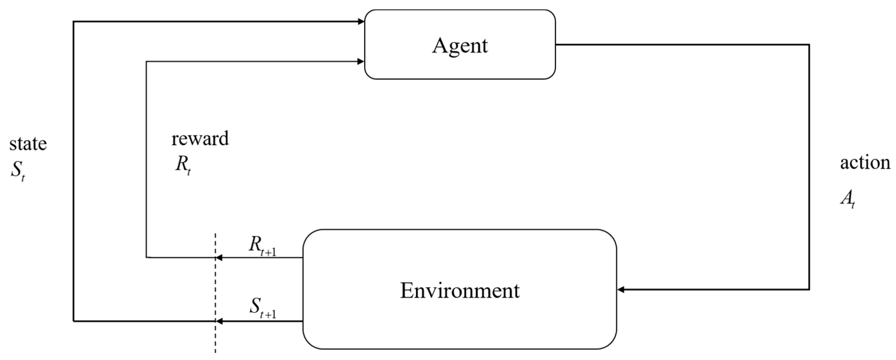
The interaction relationship between the agent and the environment is shown in Figure 1. Decision makers are called agents. The interaction with the agent is called the environment. At each step, the agent receives a number from the environment, called a reward. Rewards are short-term. The only goal of the agent is to maximize the total reward accumulated over time. Value refers to all the rewards that the agent can expect to accumulate in the future, starting from the current state. Rewards can only show immediate liking for the environment. The value function can show long-term performance. The value function is the one that shows long-term good and bad and takes into account possible future states and the rewards that can be obtained from these future states. Therefore, we have to maximize the value function.

In Figure 1, the agent interacts with the environment in a series of steps. In every step, the agent receives the state S_t of the environment and uses it to choose an action A_t. Then, in the next step, the agent receives a reward R_t+1.

Part of the reward comes from the result of the action, and part of it comes from finding oneself in a new state. The MDP and the agent together produce a sequence: S₀, A₀, R₁, S₁, A₁, R₂, etc. Assuming this sequence is finite, the random variables R_t and S_t have defined probability distributions. The distribution depends only on previous states and actions. We can say that, given the previous state and action, for specific values s′ ∈ S of the random variables, the probability of occurrence at step t is:

$$p\left(s^{\prime }|s,a\right)\equiv \mathrm{Pr}\left\{S_t=s^{\prime }|S_{t-1}=s,A_{t-1}=a\right\}$$

(1)

where Pr is the probability of a random variable. Function p indicates the probability distribution brought by s and a:

$${\displaystyle \sum _{s^{\prime }\in S}{\displaystyle \sum _{r\in R}p\left(s^{\prime }|s,a\right)=1}}$$

(2)

In every step, the agent gets reward R_t. The agent’s goal is to maximize the reward received. It is not the immediate reward that needs to be maximized, but the long-term accumulated reward. For this purpose, we define a total return function G_t:

$$\begin{array}{ll}{G}_t& \equiv R_{t+1}+\gamma R_{t+2}+{\gamma }^2{R}_{t+3}+{\gamma }^3{R}_{t+4}+\cdots \\ & =R_{t+1}+\gamma (R_{t+2}+\gamma R_{t+3}+{\gamma }^2{R}_{t+4}+\cdots )\\ & =R_{t+1}+\gamma G_{t+1}\end{array}$$

(3)

where γ is the discount rate, 0 ≤ γ ≤ 1.

Next, we discuss the policy and the value function. A policy is a mapping from states to form probabilities of choosing each possible action. Assuming the agent follows π at t, then t is the probability of A_t = a at S_t = s. The value function of state s under policy π, denoted as v_π(s), refers to the expected return from state s and following policy π thereafter. In MDP fashion, we can define v_π(s) as the following:

$$v_{\pi }(s)\equiv E_{\pi }\left[G_t={\displaystyle \sum _{k=0}^{\infty }{\gamma }^k{R}_{t+k+1}}|S_t=s\right]$$

(4)

where E_π is the expected value of the random variable when the agent follows policy π. We call function v_π the state-value function of policy π. Similarly, denoting the value of taking action a in state s under policy π as q_π(s, a) means starting from state s and taking action a, then following the expected return of policy π:

$$q_{\pi }(s,a)\equiv E_{\pi }\left[G_t={\displaystyle \sum _{k=0}^{\infty }{\gamma }^k{R}_{t+k+1}}|S_t=s,A_t=a\right]$$

(5)

We call q_π the action-value function of policy π. G_t from (3) is substituted into Equation (4), so that for any policy π and any state s, we have

$$v_{\pi }(s)\equiv E_{\pi }\left[G_t|S_t=s\right]={\displaystyle \sum _a\pi \left(a|s\right){\displaystyle \sum _{s^{\prime }}{\displaystyle \sum _{r}p\left(s^{\prime }|s,a\right)\cdot }}}$$

(6)

Equation (6) is the Bellman equation of v_π. It expresses the relationship between a state value and its successor state value. The Bellman equation averages all probabilities, weighing each chance by its occurrence. The value of one state must be equal to the discounted expected value of the next state plus the expected reward along the way.

In all states, the expected return of policy π is greater than or equal to that of all policies π′, thus policy π is defined to be better than or equal to policy π′. Policy π is an optimal policy. Let π* denote all optimal policies. These optimal policies have the same state-value function, called the optimal action-value function, denoted as v*, and defined as:

$$v*\left(s\right)\equiv \underset{\pi }{\max }{v}_{\pi }\left(s\right)$$

(7)

The best policies also have the same optimal action-value function, denoted as q*, and are defined as:

$$q*\left(s,a\right)\equiv \underset{\pi }{\max }{q}_{\pi }\left(s,a\right)=E\left[R_{t+1}+\gamma v*\left(S_{t+1}\right)|S_t=s,A_t=a\right]$$

(8)

Since v* is the value function under a certain policy, (6) must be satisfied. Besides, since it is the optimal value function, it can be presented without reference to any particular form of policy. Therefore, we can further modify (7) as:

$$v*\left(s\right)=\underset{a}{\max }{\displaystyle \sum _{s^{\prime },r}p\left(s^{\prime }|s,a\right)\left[r+\gamma v*\left(s^{\prime }\right)\right]}$$

(9)

This formula, called the Bellman optimality equation, expresses that under the optimal policy, the state value must be equal to the expected return of the state’s optimal action.

2.2. MDP-Based Path Planning

Since the Markov decision process is a discrete-time stochastic control process, in this study we first discretized the map into an occupancy grid map. A grid divides a continuous space of a certain size. The state of the agent is represented by s, which represents the coordinates $s(x_s,y_s)$ at a particular location. In other words, the set of this state is all the spaces where the agent can appear in the map. In order to simplify the operation, we discretize the map into an occupancy grid map so that S is a finite set, where m and n correspond to the height and width of the map, respectively:

$$S=\left\{s_1\left(x_{s_1},y_{s_1}\right),s_2\left(x_{s_2},y_{s_2}\right),\cdots ,s_{m\times n}\left(x_{s_m},y_{s_n}\right)\right\}$$

(10)

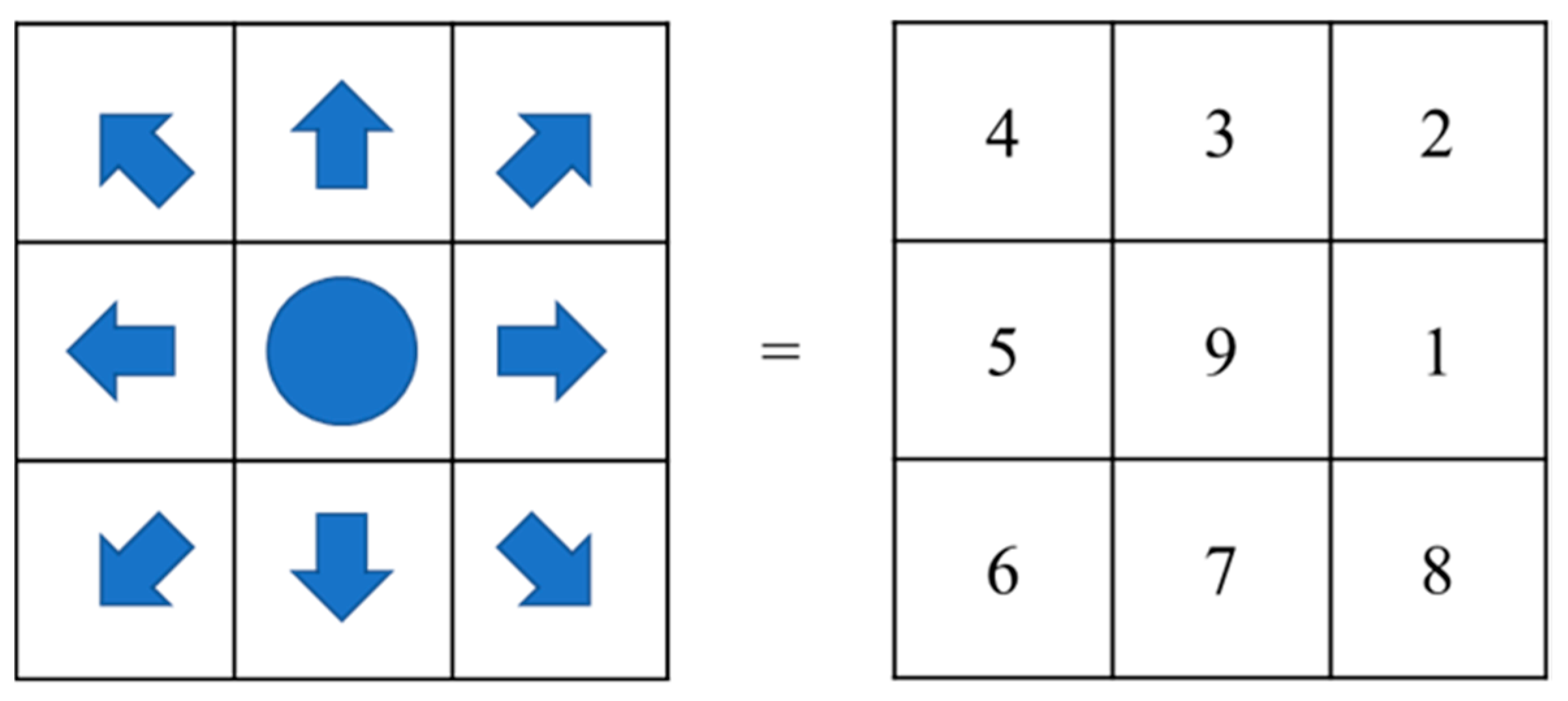
The value function of an agent at a specific location is represented by v_π(s). The higher the value of the value function, the closer the location is to the end point. The agent has u actions A = {a₁, a₂, …, a_u}. However, the actions of the agent are not completely reliable. Sometimes the agent will perform incorrect actions and have unexpected results. For example, when the agent was ordered to “go right” it actually ran to the “upper right” position. Although we cannot guarantee what actions the agent will perform in the end, we can at least know the actions and probabilities that all agents may perform after the order is given, that is, given π and all possible a, the corresponding probability is π(a|s).

2.3. Cost to Obstacles and Walls

In order to avoid the mobile robot being too close to the wall in reality, the path planned in the path planning should avoid being too close to the wall. Moreover, because the environment in which the agent is situated not expected to be too comfortable, each step will have a passing cost so that the agent can find the most suitable path as soon as possible. Therefore, we add a travel cost function z(s) to Equation (9). The modified version is given as follows:

$$v*\left(s\right)=z\left(s\right)+\underset{a}{\max }{\displaystyle \sum _{s^{\prime },r}p\left(s^{\prime }|s,a\right)\left[r+\gamma v*\left(s^{\prime }\right)\right]}$$

(11)

z(s) is the travel cost at the location of the state, and can be expressed as:

$$z\left(s\right)=k_z\cdot \max {\left(d_{\max }-d(s),1\right)}^{\alpha }$$

(12)

where k_z < 0 is the basic cost, d(s) is the distance from the position of state s to the nearest wall, α ≥ 1 is used to adjust the influence magnitude near the wall and d_max is the critical value of d(s). If d_max − d(s) ≤ 1, the attenuation of the value function is only the basic cost k_z. On the other hand, if the position is too close to the wall and d_max − d(s) > 1, then this cost increases with the power of α.

Next, there must be moving obstacles in the dynamic environment, so we designed a function c(o, s). First, we define o as the observable moving obstacle in the environment, so its coordinate is known as o(x_o, y_o), and the set O = {o₁, o₂, …, o_w} represents this group, and the number is w. Then, we define c(o, s) as the influence of the obstacle o on the state s, and use this to modify Equation (11) to obtain:

$$v*\left(s\right)=z\left(s\right)+\underset{a}{\max }{\displaystyle \sum _{s^{\prime },r}p\left(s\right)\left[r+\gamma v_{*}\left(s^{\prime }\right)\right]}+{\displaystyle \sum _{o\in O}c\left(o,s\right)}$$

(13)

The formula for c(o, s) is given as follows:

$$\begin{array}{l}c\left(o,s\right)=k_d\cdot \max \left(r_{\max }-r\left(o,s\right),0\right)\\ r\left(o,s\right)={\left(x_o-x_s\right)}^2+{\left(y_o-y_s\right)}^2\end{array}$$

(14)

where k_d < 0 and r_max is the critical value of r(o, s).

2.4. Dynamic Programming

Dynamic programming refers to a series of algorithms for computing the optimal policy given the complete the environment model as MDP. If the environmental dynamics are completely known, then Equation (13) is a system in which |S| linear equations and |S| unknowns exist simultaneously. For this reason, an iterative solution is the most suitable method. v₀ is initialized, and each subsequent value is then calculated by using the modified Bellman equation in Equation (13) with the updated rule for all s ∈ S:

$$v_{k+1}\left(s\right)=z\left(s\right)+\underset{a}{\max }{\displaystyle \sum _{s^{\prime },r}p\left(s^{\prime }|s,a\right)\left[r+\gamma v_k\left(s^{\prime }\right)\right]}+{\displaystyle \sum _{o\in O}c\left(o,s\right)}$$

(15)

Obviously, v_k = v* is a fixed point under this rule because the Bellman equation of v* can guarantee the equality sign. As long as v* is guaranteed to exist under the same conditions, the sequence {v_k} will converge to v* along with k→∞. This algorithm is called value iteration. To obtain each successor v_k+1 from v_k, iterative policy evaluation takes the same action for each state s and replaces state s with a new value consisting of the old value of state s and its successor state and the expected immediate reward (called “expected update”). Each iteration updates the value of each state to produce a new approximation function v_k+1.

We compute the value function of a policy in order to find a better policy. Assuming that an arbitrary deterministic value function v_π has been determined, for some state s, we want to know whether we need to change the policy to choose an action a which is not π(s). One way to solve this problem is to consider choosing action a from state s and then follow the existing policy π. The value obtained in this way is:

$$q_{\pi }\left(s,a\right)\equiv E\left[R_{t+1}+\gamma v_{\pi }\left(S_{t+1}\right)|S_t=s,A_t=a\right]={\displaystyle \sum _{s^{\prime },r}p\left(s^{\prime }|s,a\right)\left[r+\gamma v_{\pi }\left(s^{\prime }\right)\right]}$$

(16)

A key criterion is whether the above formula is greater or less than v_π(s). If greater, it is better to follow the policy π after the state s chooses the action a once than to follow π all the time. In this case, we can expect that it is better to choose action a every time that state s is reached. If the statement is satisfied as follows:

$$q_{\pi }\left(s,{\pi }^{\prime }\left(s\right)\right)\ge v_{\pi }\left(s\right),\forall s,\pi ,{\pi }^{\prime }$$

(17)

then policy π′ must be the same or better than policy π. That is, policy π′ must achieve better or equal expected returns from all states s ∈ S:

$$v_{{\pi }^{\prime }}\left(s\right)\ge v_{\pi }\left(s\right)$$

(18)

From this we learn that, given a policy and value function, we can easily evaluate the change. Therefore, we can naturally extend to all states and all possible action changes, choosing the best action according to q_π(s, a) in each state to a specific action under this policy. In other words, considering a new greedy policy π′, then:

$${\pi }^{\prime }\left(s\right)\equiv \arg \max q_{\pi }\left(s,a\right)=\underset{a}{\arg \max }{\displaystyle \sum _{s^{\prime },r}p\left(s^{\prime }|s,a\right)\left[r+\gamma v_{{\pi }^{\prime }}\left(s^{\prime }\right)\right]}$$

(19)

The greedy policy performs a single-step search based on v_π and takes action a that looks best in the short term. If the structure satisfies Equation (17), it can be known that this policy is the same as or better than the original policy. The process of formulating a new policy to improve the original policy in a greedy manner from the value function of the original policy is called policy improvement.

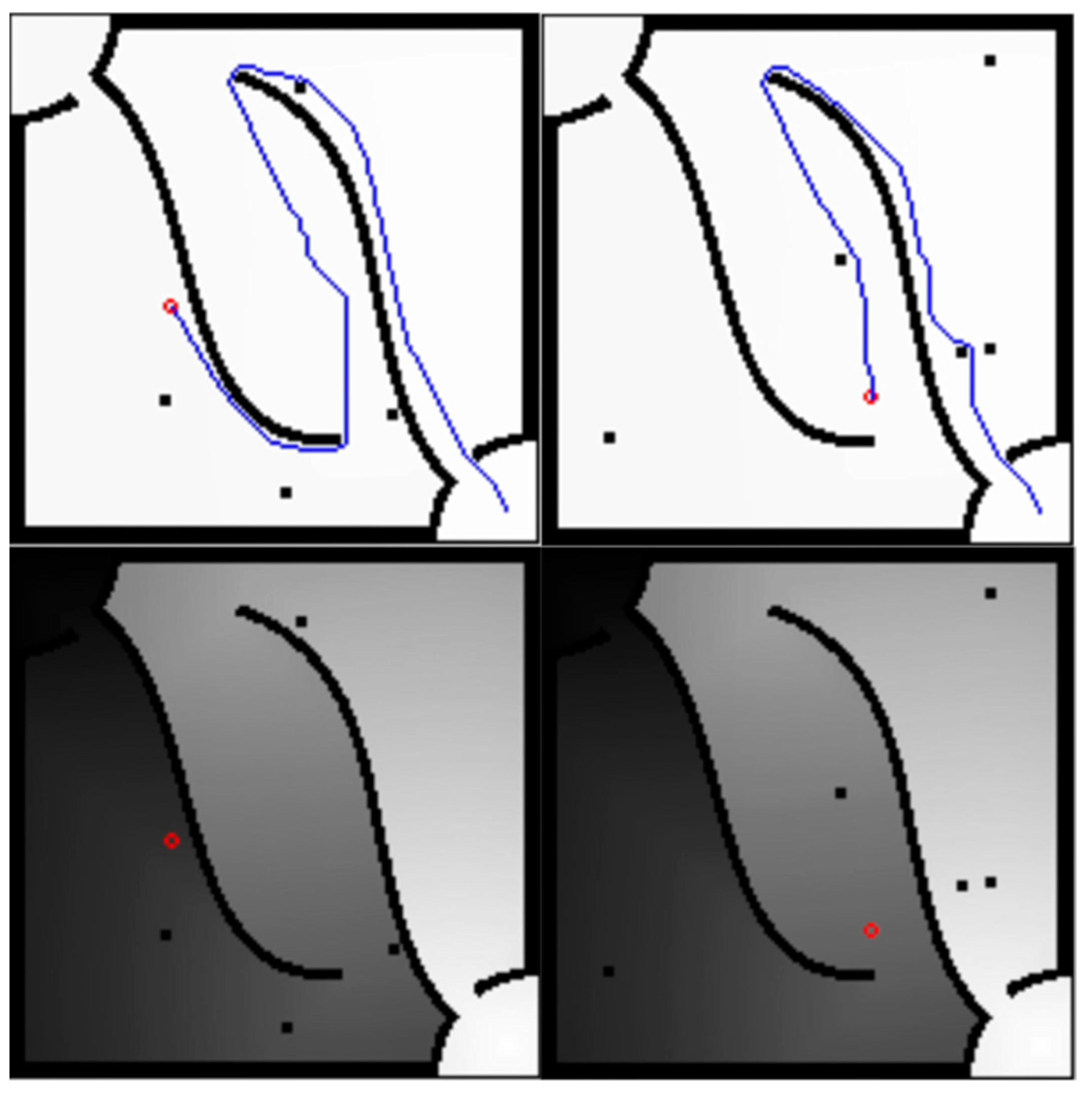
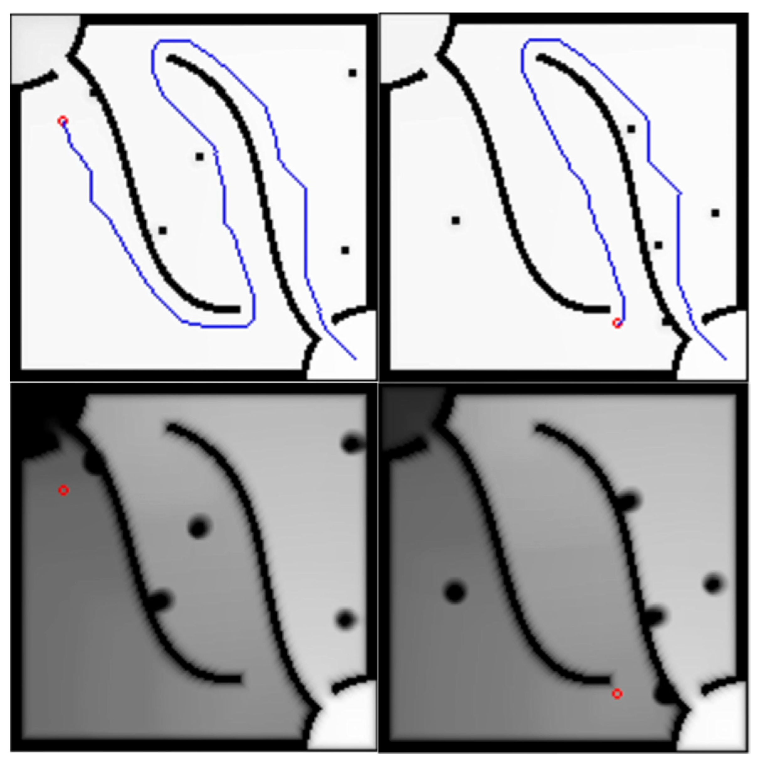
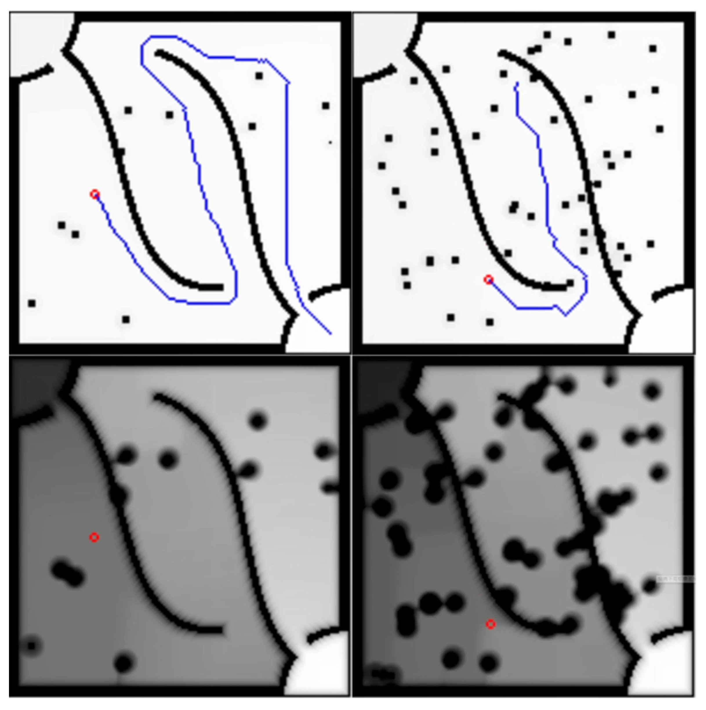
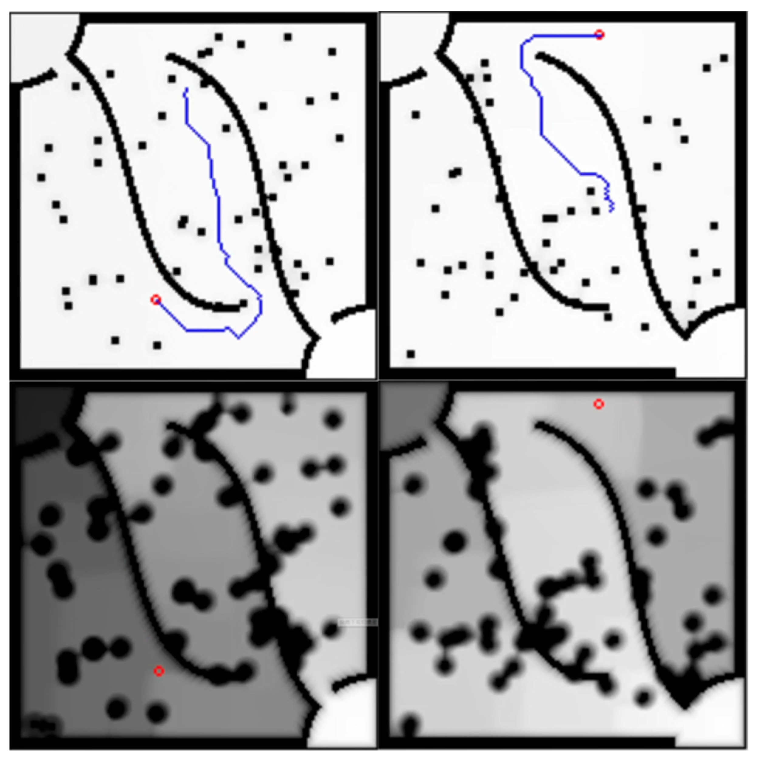
Once policy π improves using v_π and produces a better policy π′, we can compute v_π′ and improve the policy again to obtain a better policy π″, thus obtaining a series of policies and value functions that continue to improve. All states can be obtained through Formula (19) to obtain the optimal behavior at that location, but it is not necessary to solve all states (because the value function will change with the environment), so the optimal behavior obtained at the moment is not fit for the future. In fact, just by substituting the state s_c(x_sc = x_c, y_sc = y_c) of the corresponding agent position c_k(x_c, y_c) into Equation (19), the policy π_k(s_c) can be obtained, and then the agent will go to s_c′. s_c′ can be substituted into formula (19) again to obtain the policy corresponding to the position of s_c′ to form a loop iteration to solve step by step. If π_k(s_c′), s_c″, π_k(s_c″), s_c‴, s_c‴, π_k(s_c‴), s_c⁽⁴⁾, … are continuously obtained in a single time point in the same steps. It will reach a state s_c^(g) at the end point. At this time, the coordinates corresponding to [s_c, s_c′, …, s_c^(g)] are the paths that the agent can go to the end point at this time and guide the agent to the end point. A series of policies is [π_k(s_c), π_k(s_c′), …, π_k(s_c^{(g − 1)})]; if s_c′ is substituted into (5) at the next time point, π_k(s_c′), then the whole process will be transformed into the guidance mechanism of the agent, so that the agent will obtain a policy corresponding to the position at each time point, and this policy will change with the map and transform into [π_k(s_c), π_{k + 1}(s_c′), …, π_{k + h − 1}(s_c^{(g − 1)})], but it still eventually leads the agent to the end. Since the latest utility value is used every time a new policy is established, and the value function covers the influence from the agent’s behavioral ability, and from the static and dynamic obstacles, this method can achieve good performance in complex environments.

2.5. Time Complexity Analysis

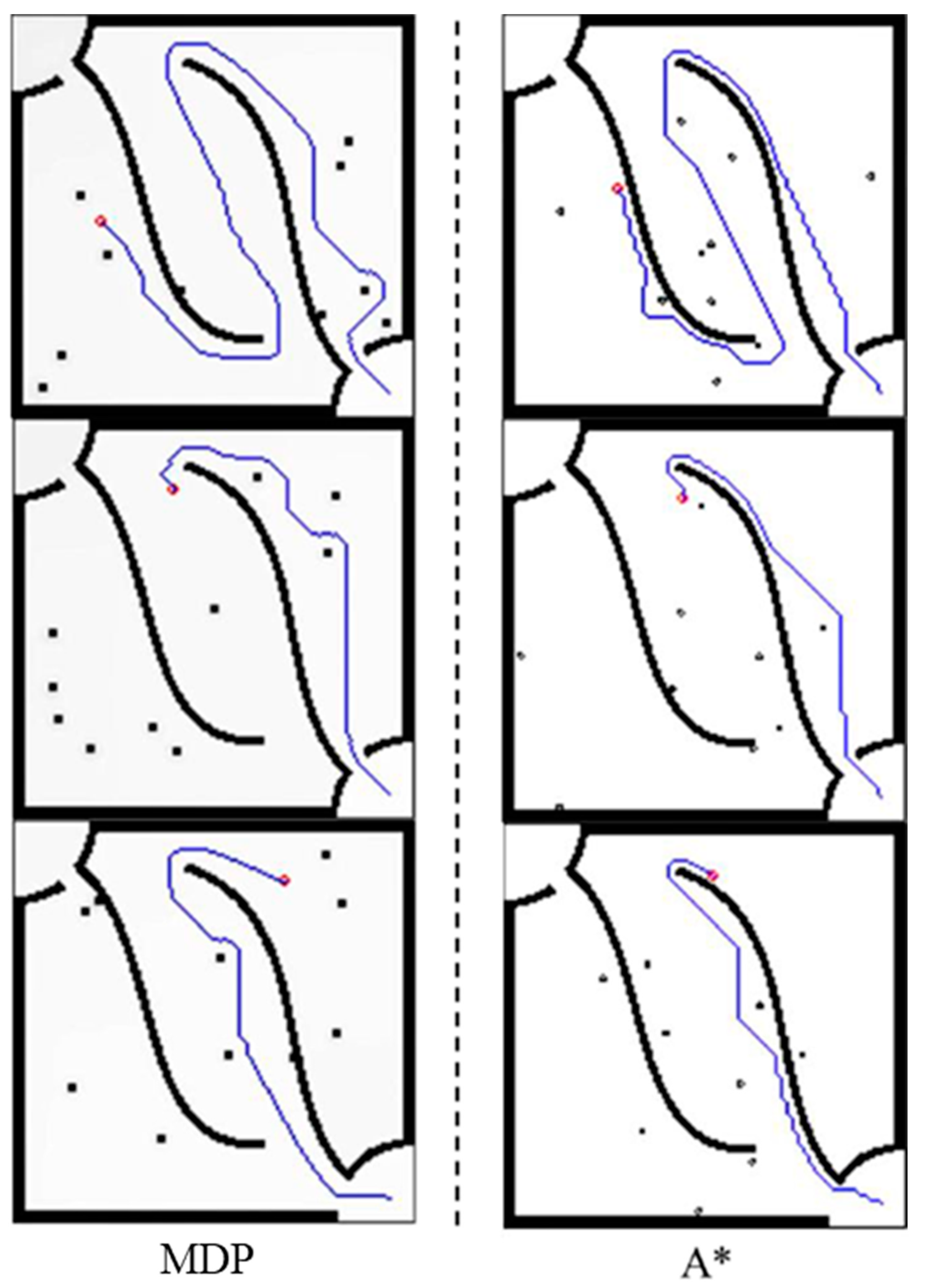
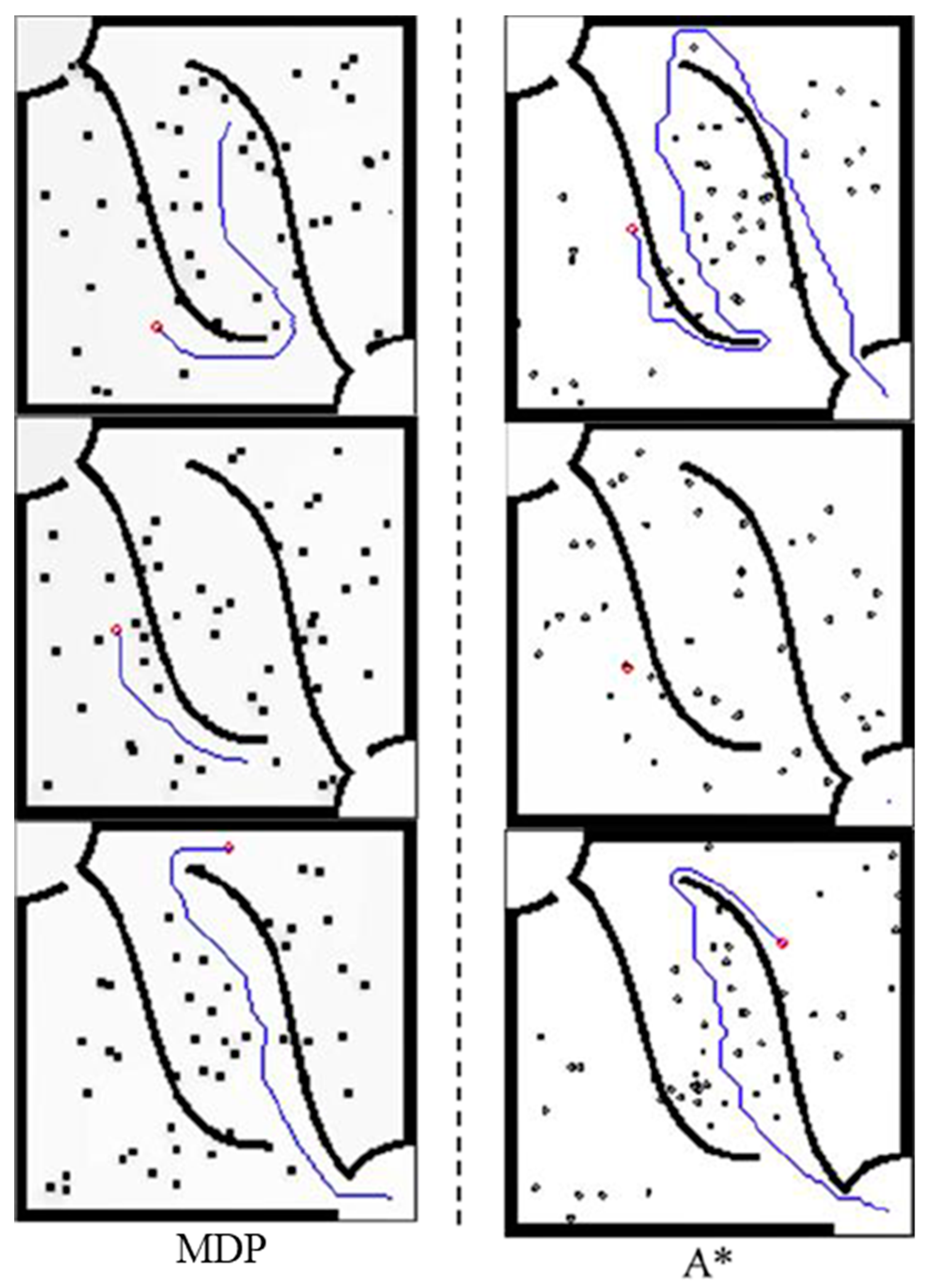
In addition to the above-mentioned differences in path planning, the execution time of the two algorithms on this map will be analyzed here. The method provided in this thesis is divided into two parts: value iteration and path finding. The A* algorithm performs path finding by searching for the target and calculating the path.

Table 1. Algorithm analysis between the proposed and A* algorithm.

	Completeness	Optimality	Time Complexity	Suitable for Dynamic Environments
Proposed algorithm	yes	yes	First path: O(n2) After second path: O(n)	yes
A* algorithm	yes	yes	Average: O(nlogn) Best: O(n)	no

compares some characteristics of the method (MDP) of this paper and the A* algorithm, such as completeness, optimality, time complexity, whether it is suitable for dynamic environments, etc. Both completeness and optimality are only analyzed in static environment, because moving obstacles are considered unpredictable in this paper. It can be seen that when generating the first path, the time complexity is O(n²), which is far more than the average time complexity O(nlogn) of the A* algorithm because it is necessary to continuously iterate the value until the value function at the starting point is greater than 0. However, after the second path, only one “value iteration” and one “path finding” are required for each execution, and the time complexity is reduced to O(n). Due to this feature, it is quite suitable for execution in a dynamic environment.

3. Simulation Results

3.1. Parameter Settings

First, the most important parameter to calculate MDP is transfer model p(s′|s, a). Figure 2 is the behavior number. Then, the transfer model is represented as the following:

$$\begin{array}{l}p\left(s^{\prime }=s_i|s=s_9,a=a_i\right)=0.8,1\le i\le 8\\ p\left(s^{\prime }=s_{i+1}|s=s_9,a=a_i\right)=p\left(s^{\prime }=s_{i-1}|s=s_9,a=a_i\right)=0.1,2\le i\le 7\\ p\left(s^{\prime }=s_2|s=s_9,a=a_1\right)=p\left(s^{\prime }=s_8|s=s_9,a=a_1\right)=0.1\\ p\left(s^{\prime }=s_1|s=s_9,a=a_8\right)=p\left(s^{\prime }=s_7|s=s_9,a=a_8\right)=0.1\\ p\left(s^{\prime }=s_9|s=s_9,a=a_9\right)=1.0\end{array}$$

(20)

There is a 0.8 chance that the expected outcome will occur, but there is a 0.2 chance that the agent will move in the expected direction. The result of hitting a wall is not moving. The coordinates of the start and goal points are (10, 10) and (140, 140) respectively. The goal point is set to the aborted state and has a “+1” reward. The map size is 150 × 150 pixels. The discount rate γ is set to 1. It can be seen that when γ = 0.98, the value function has been unable to iterate until the starting point is greater than 0, so there will be no corresponding path in simulation. The parameters of the value function update are k_z = −3 × 10⁻⁵, α = 3, and d_max = 5.

3.2. Real-Time Obstacle Avoidance and Path Planning

Now we use (15) to iterate, but remove the z(s) part, and Equation (14) is modified to c(o, s) = 0, which means that only the value function of the obstacle itself is 0, and there is no additional protection. The number of obstacles is five. The results are shown in Figure 3. Figure 3 shows the real-time path planning. In the figure, the top row is the live path and the bottom row is the value function image. All the states updated by Equation (15) in the value function image are bounded in [0, 1], the value of walls and obstacles are fixed in 0 and the goal is fixed in 1. According to the update rule, the goal is the only one with highest value; hence, the path toward to the highest value, which is only the goal, can be easily found. The agent can follow the path to reach the target point and avoid obstacles in time, but we can see that the agent does not keep a certain distance from walls and obstacles, and so has a high probability of hitting walls and obstacles in reality.

Next, we use the revised Equation (15) to iterate. The calculation of distance cost is added to this formula so that the agent can keep a certain distance from walls and obstacles. The results are shown in Figure 4. Compared with Figure 3, it can keep a certain distance from walls and obstacles. The value of any state too close to the walls and obstacles are significantly reduced relative to neighboring state. In Figure 5, we show real-time path planning for 10 and 50 obstacles. We found that, in complex environments with many obstacles, the agent can still effectively plan paths and avoid walls and obstacles. Although the path shows that the goal cannot be reached at all time points, it can effectively guide the agent in the direction of the destination. Finally, we try to change the map when the agent is approaching the end point, as shown in Figure 6. We can see that valid paths are still found in real time when the map changes. During the entire movement process, the agent can always keep enough distance from the obstacles or walls.

The simulations of the proposed MDP path planning algorithm with different number of obstacles will be shown in Figure 7 and Figure 8 and compared with the A* algorithm path planning. It can be seen that in the two figures, the A* path planning algorithm must ensure that all paths are passable before the end point can be planned. However, the MDP method used in this study does not necessarily have to search for the end point to generate a path. Like the part of the MDP in Figure 8, the path is not generated to the end and can be moved immediately because when using the MDP method to replace the value function with the starting point, the agent basically already knows the dynamics of the entire environment. It is therefore not necessary to follow the value function to give a new path trend, as it will be correct, and it does not have to be updated to the end. However, this is not the case with the A* algorithm. The agent of the A* algorithm does not understand the dynamics of the entire environment every time it recalculates, so it must find the end point when calculating the path. This also causes the agent to stay in place once there is no way to find the path to the end point. This way, the agent will be hit directly by the moving obstacle. However, the method in this paper will reduce the value function because the grids around the moving obstacles will cause the planned path to actively avoid these moving obstacles. This is also one of the advantages of this method.

Another advantage in this study is that it inherits the advantage of MDP.

Table 2. No moving obstacles in the environment.

	Value Iteration	Path Finding (ms)	Total Time after 2nd Path (ms)
Proposed algorithm	After 2nd path: 6.86 (every iteration)	0.12	6.98 (6.86 + 0.12)
A* algorithm	--	17.50	17.50

,

Table 3. The environment contains 5 moving obstacles.

	Value Iteration	Path Finding (ms)	Total Time after 2nd Path (ms)
Proposed algorithm	After 2nd path: 7.20 (every iteration)	0.09	7.29 (7.20 + 0.09)
A* algorithm	--	17.54	17.54

,

Table 4. The environment contains 10 moving obstacles.

	Value Iteration	Path Finding (ms)	Total Time after 2nd Path (ms)
Proposed algorithm	After 2nd path: 7.30 (every iteration)	0.11	7.41 (7.30 + 0.11)
A* algorithm	--	18.10	18.10

and

Table 5. The environment contains 50 moving obstacles.

	Value Iteration	Path Finding (ms)	Total Time after 2nd Path (ms)
Proposed algorithm	After 2nd path: 7.43 (every iteration)	0.19	7.62 (7.73 + 0.19)
A* algorithm	--	18.13	18.13

show the time used in the map of 150 × 150 pixels, 5, 10 and 50 mobile obstacles, respectively. Among them, the time required by the MDP method is the secondly generated path, including the cost form value iteration and path finding. When the MDP is generating the first path (since the value function has always been iterated to the starting point position), it will only find the path according to the value function of the entire map, so the time will cost more. At this point, the time is about 11 s.

The results in Table 2, Table 3, Table 4 and Table 5 all show that after the agent starts to act, the method provided in this paper has a considerable advantage in the execution time of the next path to be found in response to the dynamic environment after iterating the first path. Moreover, the two parts of the Markov decision process path planning algorithm, value iteration and path search can be executed separately, which means that if these two parts are separately processed by different cores of the computer, the time to find the path is only about 0.2 milliseconds.

Combining the above two differences, it can be seen that the Markov decision process path planning algorithm is significantly better than the A* algorithm in a dynamic and complex environment, whether it is in execution time, avoiding moving obstacles, or adapting to dynamic environments.

3.3. Comparison and Discussion of Different γ Values

The discretized grid map used in this paper has only a limited number of grids, so setting the discount rate γ = 1 will not make the expected total reward accumulation positively or negatively infinite, and the discount rate can be understood as the agent’s comparison of the current return with the future return preferences over future rewards. When γ is close to 0, far future rewards are considered to be insignificant. Therefore, the smaller the value, the more prone to “short-sightedness.” Figure 9 shows the simulations when γ = 0.98, 0.99 and 0.995, respectively. It can be seen that when γ = 0.98, the value function is unable to iterate until the starting point is greater than 0, so there will be no corresponding path in this simulation. When γ = 0.99 and 0.995, there is not much difference from the planned path when γ = 1, so γ = 1 is used in this experiment.

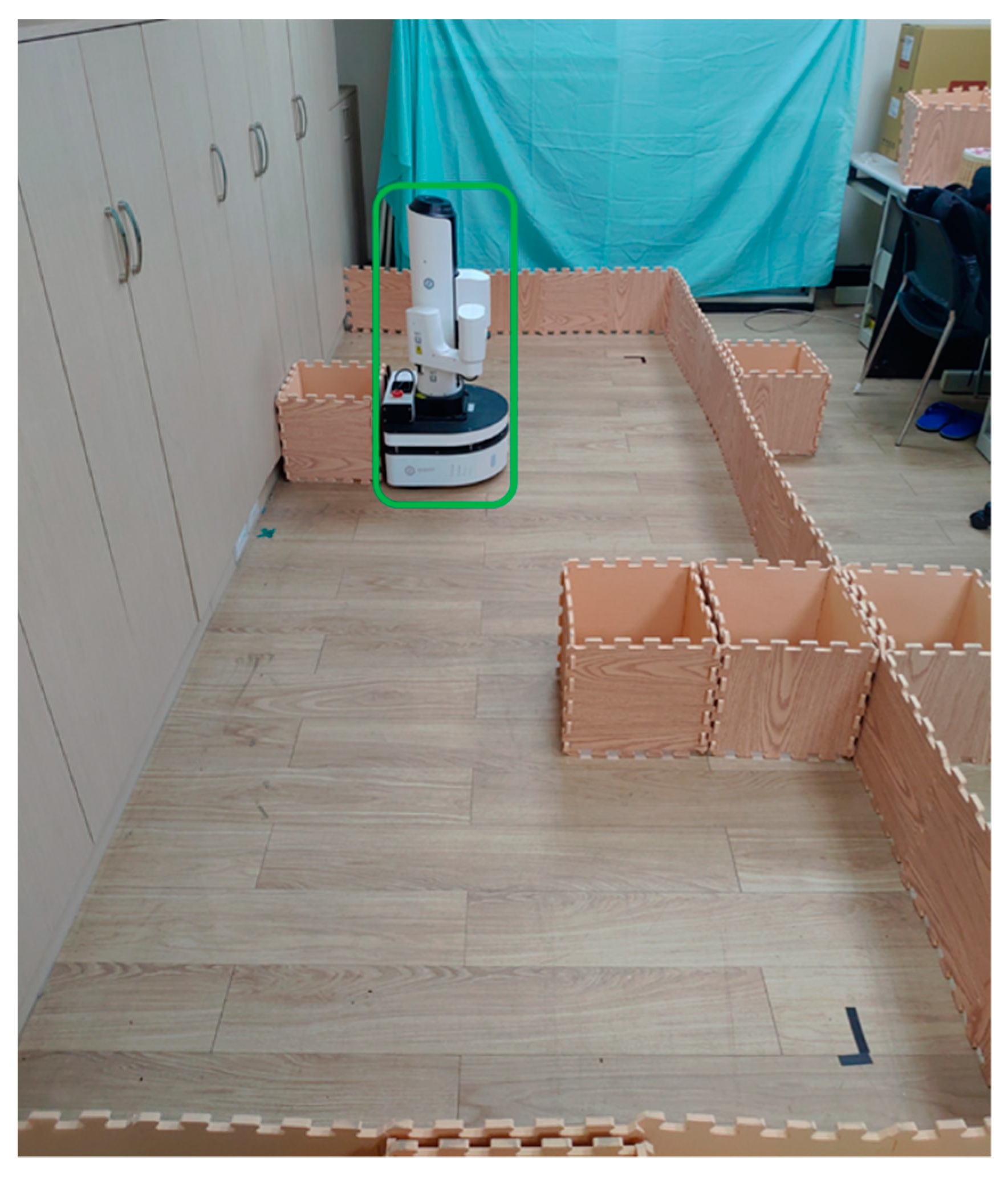
4. Experimental Results

This section reports the experiments conducted on mobile robots in practical applications. The experiments are divided into test items such as no obstacles, fixed but unknown obstacles, moving unknown obstacles, and people walking constantly, and they are compared with the A* algorithm. This path planning experiment uses ROS, so the navigation package in ROS must be rewritten. The one to be rewritten is nav_core::BaseGlobalPlanner in ROS. After ROS gets the path, it will use the built-in path tracking algorithm to move. 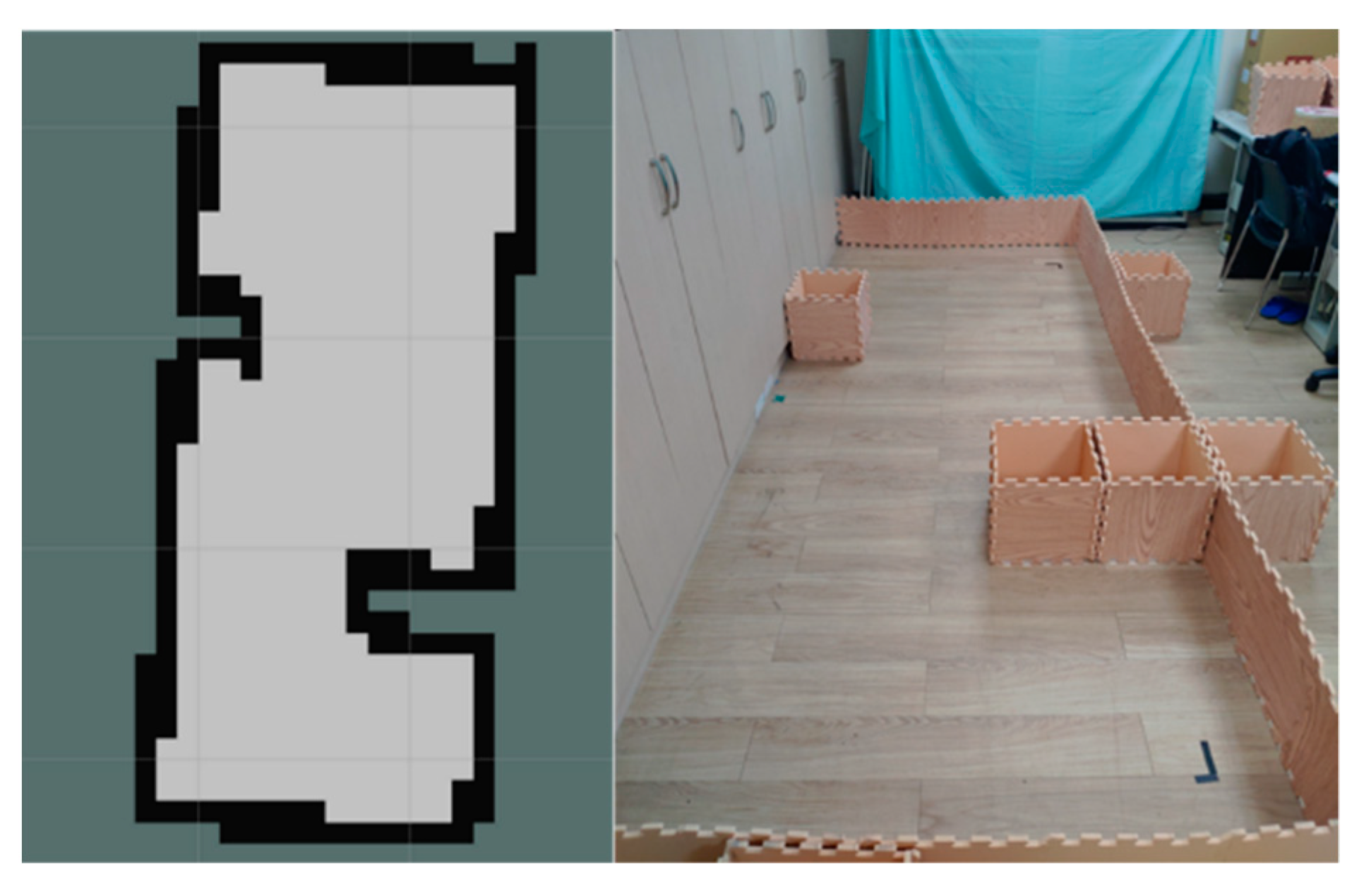Figure 10 is the map of this experiment, and the left side of the picture is the result of SLAM on the actual field on the right side. The starting point is in the lower right corner of the picture, and the target point is in the upper left corner of the picture. On the left is the picture from SLAM. The size of the map is about 3 × 1.8 m, the resolution is 0.1 m/pixel, and then the pixels are used as the discretized grid map. After the output path is sent to ROS, the system will automatically adjust the path to make it smoother. Among them, the parameters are given as k_z = −3 × 10^–3, k_d = −0.1, α = 1, d_max = 3 and r2_max = 3.

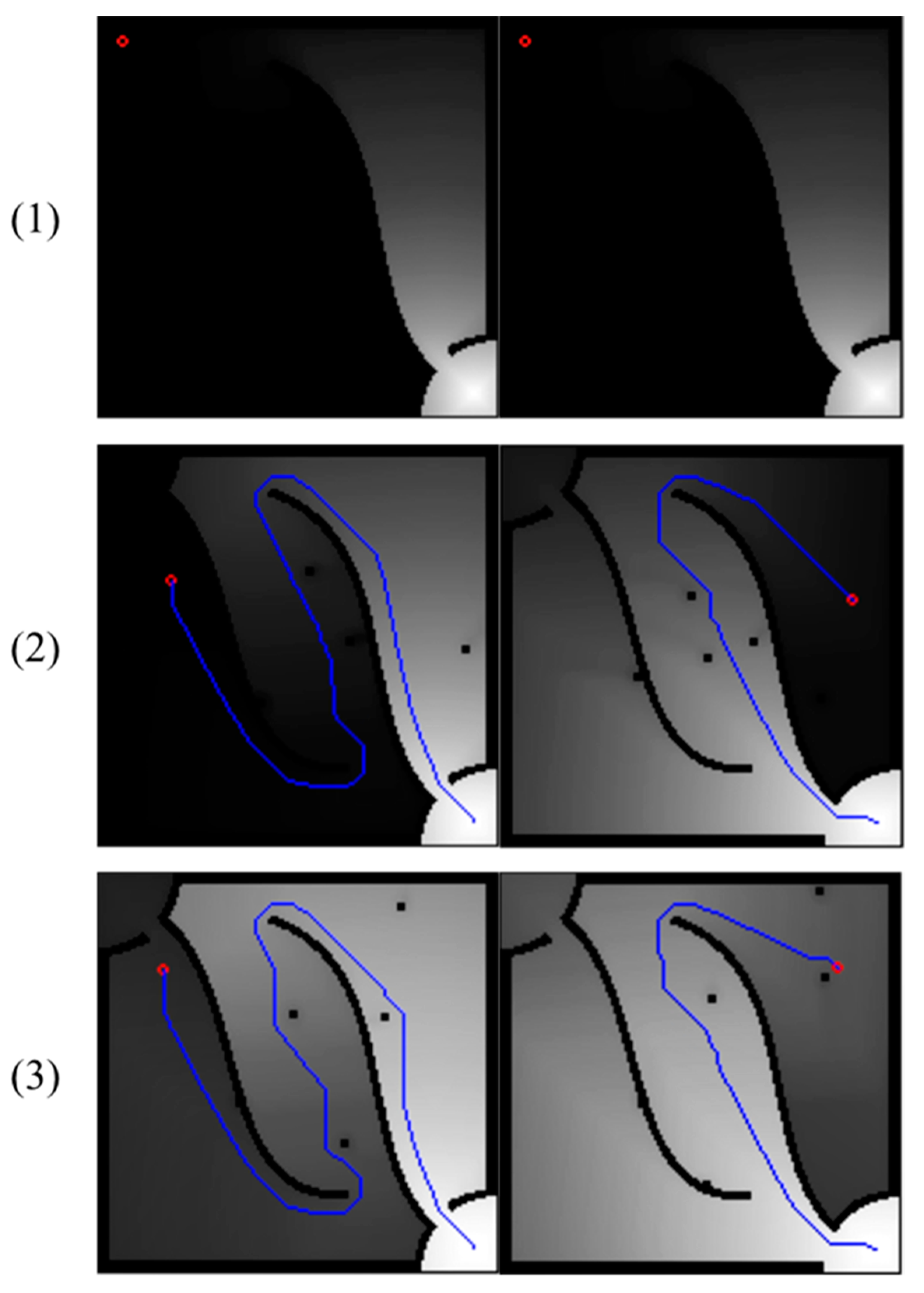
The first experiment is a test without unknown obstacles; Figure 11 shows the Markov decision process path planning algorithm, where the red dots are the obstacles scanned by the Lidar, the green lines are the paths and the green arrows are the point distributions of the built-in AMCL.

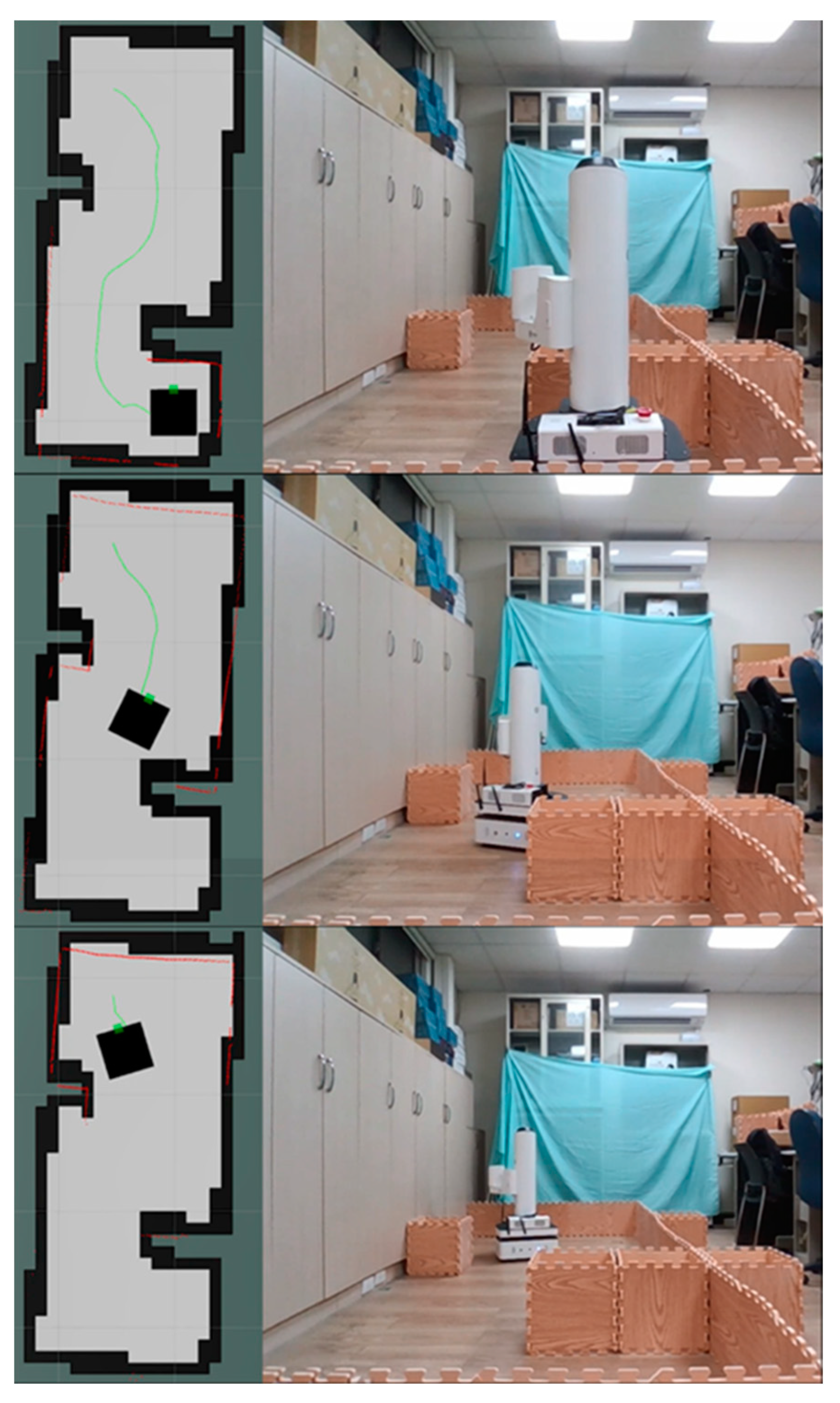
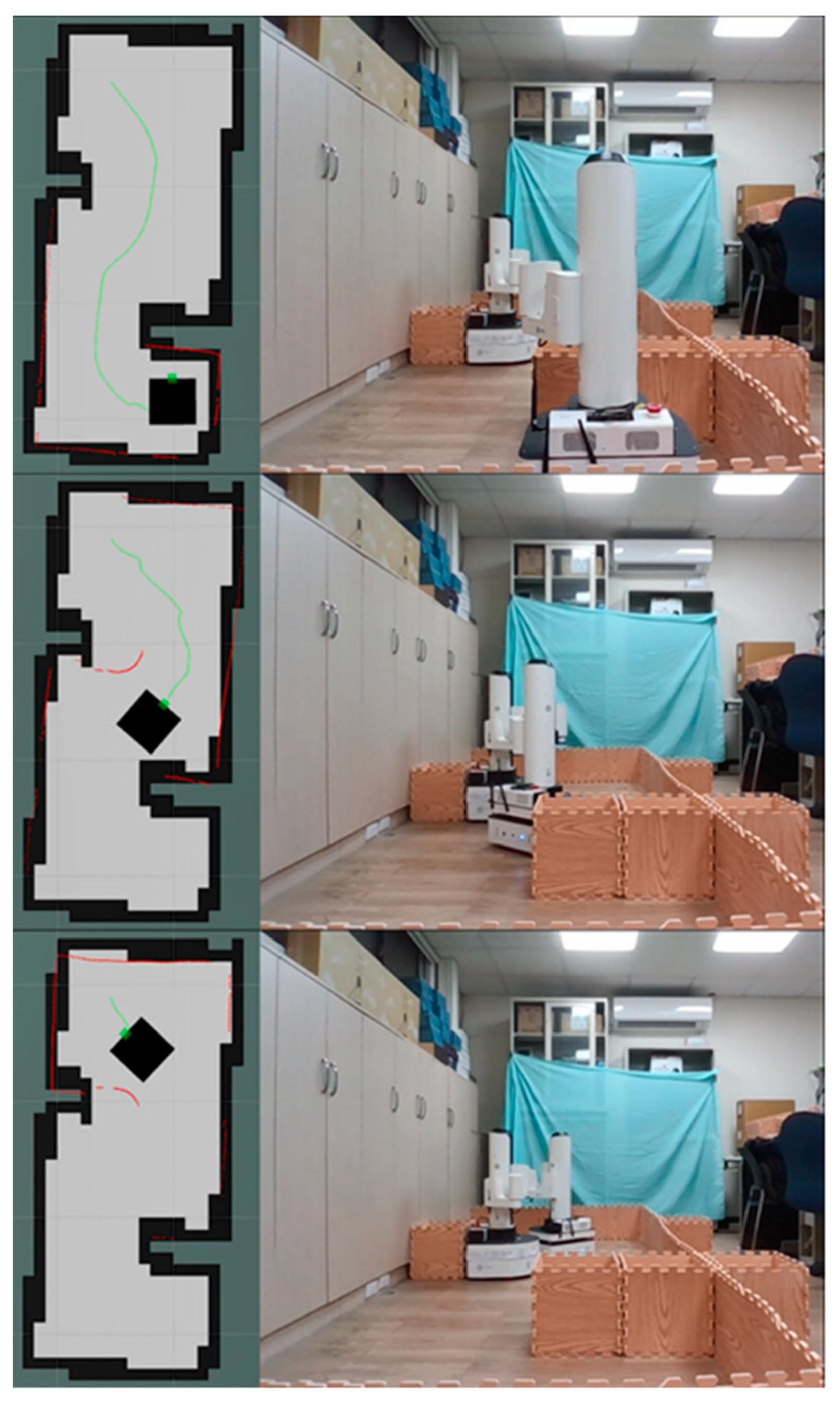
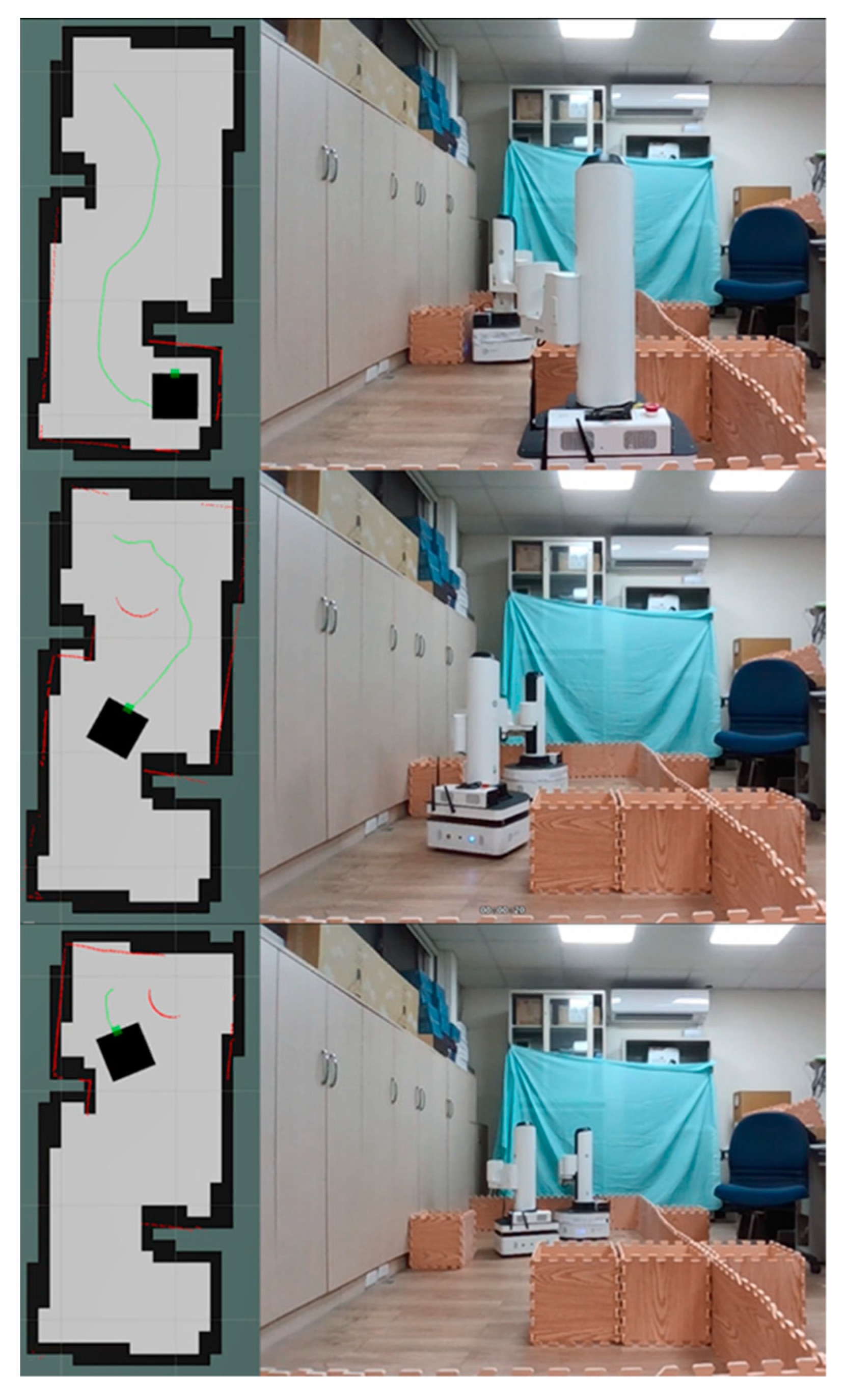
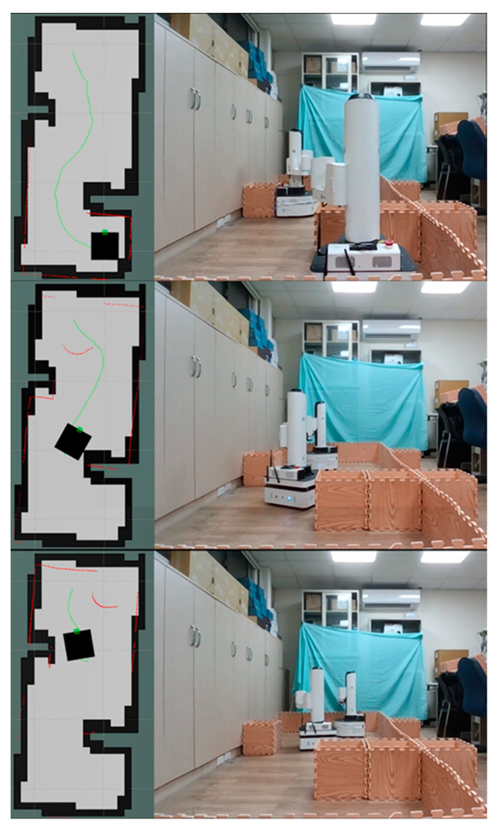
In the second experiment, the unknown fixed obstacles are shown in Figure 12, and the test with unknown but fixed obstacles is shown in Figure 13. In the third experiment, a test with unknown moving obstacles is carried out. The unknown moving obstacles are the same as those shown in Figure 12 and are moved. Figure 14 and Figure 15, respectively, show the Markov decision process path planning algorithm and the A* algorithm. This mobile obstacle is another mobile robot, which moves in the environment and is operated artificially. In this experiment, it was found that the A* algorithm experienced some delay, but it should be within the error range.

The above experiments started from the situation of “no unknown obstacles at all,” and continued to the situations of “fixed obstacles” and “moving obstacles.” It can be seen that the Markov decision process path planning algorithm can find the correct path, and when there are moving obstacles and people, they can also avoid them in real time, and quickly recalculate and plan a new path. There is almost no difference from the A* algorithm when there are no unknown obstacles and fixed obstacles at all, but in the situation where there are moving obstacles and moving people, there is a little delay when changing the route.

5. Conclusions

This research proposes a path planning algorithm based on the Markov decision process for wheeled mobile robots. Starting from listing the general formula of Bellman’s optimal equation and dynamically programming to find the general mathematical equation, the path planning algorithm is proposed with two update phases, namely utility and policy updates. With the travel cost function given in the utility update rule, the planned path always keeps a certain distance from the walls and obstacles, no matter whether they are fixed or moving. Compared with the A* algorithm, the proposed algorithm has better performance with moving obstacles, because it takes a much shorter time to update the path. If the moving obstacles are too close to the robot, the utility value will drop rapidly, and will therefore push the robot far away from the moving obstacles. In a complex environment, such as the case with 50 moving obstacles, the obstacle avoidance performance may decrease because of rigorous path planning to the goal, so that the robot has no time to react and collides with obstacles, which often happens with the A* algorithm. The proposed path planning algorithm is also run in ROS and then applied to industrial mobile robots. The results demonstrate the effect of real-time obstacle avoidance.