Article

Target Tracking of Snake Robot with Double-Sine Serpentine Gait Based on Adaptive Sliding Mode Control

1
School of Automation Science and Engineering, South China University of Technology, Guangzhou 510641, China
2
The Key Laboratory of Autonomous Systems and Networked Control, Ministry of Education, Unmanned Aerial Vehicle Systems Engineering Technology Research Center of Guangdong, South China University of Technology, Guangzhou 510641, China
*
Author to whom correspondence should be addressed.
Actuators 2023, 12(1), 38; https://doi.org/10.3390/act12010038
Submission received: 27 November 2022 / Revised: 6 January 2023 / Accepted: 8 January 2023 / Published: 10 January 2023
(This article belongs to the Special Issue Applications of Intelligent Control in Actuators Systems)

Abstract

:
This paper studies the target tracking control strategy of a snake robot and proposes an adaptive sliding mode control method. The strategy ensures the robot follows the target path by controlling the joint angle through feedback, pushing the robot to reach the target position through gait function. In order to achieve target tracking, a kinematic model of a snake robot was first established in this paper. Then, we used double-sine serpentine gait to solve the problem of low steering efficiency caused by regular serpentine gait, and we explored the relationship between control parameters and robot steering. On the basis of gait, in order to further improve the efficiency of target tracking for the snake robot, an adaptive sliding mode control method, based on a new sliding mode reaching law, was proposed. Finally, the effectiveness and practicability of the proposed strategy was demonstrated by comparative analysis and simulation experiments.

1. Introduction

As one of the hotspots of robot research, the bionic robot plays an important role in engineering applications [1,2,3,4]. Inspired by the biological snake, the snake robot has strong flexibility and high stability. Compared with wheeled, tracked, and legged robots, the snake robot is more adaptable to narrow and unstructured environments [5,6,7,8,9]. Therefore, it is widely used in post-disaster rescue, terrain reconnaissance and pipeline inspection [10,11,12,13,14,15].
At present, research on the snake robot mainly includes mechanical structure, motion gait, motion control method and algorithms related with robot vision information. The snake robot usually adopts a modular structure, which drives the robot forward by controlling the joint angle. In the 1940s, Gray [16] studied the locomotion of biological snakes, and used mathematical methods to describe the movement mechanism. Hirose developed the first snake robot prototype, ACM-III, in 1972 [17]. By observing a large quantity of biological snake motions, Hirose [18] proposed a serpentine gait, and added a constant offset to change the motion direction of the snake robot. Ye et al. [19,20] analyzed the serpenoid curve of the snake robot, and proposed the amplitude modulation method, the phase modulation method and the side movement modulation method to complete the turning motion of a snake robot. Dai et al. [21] referred to geometric mechanics to control a snake robot moving across a particle surface. He established an empirical model of the local relationship between change in the robot shape and position change, which could give an efficient turning gait. However, it is difficult to achieve a sharp turn of the fuselage in a narrow space with a single wave using the above studies. Inspired by the postures of Caenorhabditis elegans (C. elegans), Wang et al. [22,23] introduced a template with two coplanar traveling waves, and proposed the omega turn method to realize robot turning in place.
Motion control determines whether a snake robot can work accurately in narrow and unstructured environments, so it is necessary to study the control strategy of the snake robot [24,25,26]. Liljebäck et al. [27,28] proposed a Line-of-Sight (LOS) guidance law, and controlled the motion direction angle of a snake robot by adjusting the joint offset to realize the robot’s path tracking. Kelasidi et al. [29] proposed an integrated line-of-sight guidance law, and designed a direction controller with serpentine gait to design a trajectory tracking controller for an underwater snake robot. Ariizumi et al. [30] designed a controller based on the minimization of cost function to realize the head trajectory tracking control of s snake robot. Zhang et al. [31,32] proposed a path edge guidance strategy with the angular symmetry adjustment method to control a snake robot following the centerline of desired path. Xiao [33] adopted a sliding mode controller, based on a power reaching law, and integrated target detection technology to achieve path tracking. Cao et al. [34] analyzed the relationship between phase offset of the pitch joint and the direction of the snake robot, and proposed a control method with an adaptive LOS guidance law, which improved the tracking accuracy of the snake robot.
Although researchers have made many achievements in the motion control of the snake robot, the following problems still need to be solved: the traditional serpentine gait limiting the turning range of the robot, and the imperfect control strategy of the snake robot in target tracking, causing slow error convergence.
In order to improve the efficiency of robot target tracking, this paper proposes a target tracking control strategy based on an adaptive sliding mode controller. This control strategy drives the snake robot to change its heading angle by designing an effective feedback control law, so that the robot can quickly and stably converge to the desired path containing the target point. Meanwhile, this strategy controls the joint angle of the robot to reach the target position through the gait function. First, according to the structure of the snake robot, the kinematic model was obtained, based on screw theory. Second, considering that the target tracking process requires a lot of direction adjustment, and it is difficult to control a snake robot with many control parameters in tracking the target point, we established a double-sine serpentine gait. Third, based on the double-sine serpentine gait, an adaptive sliding mode controller was designed to achieve target tracking, and the stability of the controller was analyzed theoretically. Finally, through a simulation experiment, the tracking characteristics of the robot under different controllers were analyzed, and the effectiveness and superiority of the adaptive tracking controller, based on the double-sine serpentine gait, were verified.
Compared with existing works, the main contributions of this paper are as follows:
(1) A snake robot in regular serpentine gait, with the offset of joint angle, generates jitter when adjusting the direction angle, which causes inefficiency in controlling changes in motion direction of the snake robot. To solve the problem, this paper referred to the superposition of the two sine waves method, and established a double-sine serpentine gait model. In addition, we also analyzed the influence of each control parameter in the gait model on the movement form of the snake robot in detail.
(2) In order to further improve the tracking accuracy and convergence speed of the controller, we proposed an adaptive sliding mode controller, based on a new sliding mode reaching law, which effectively realized target tracking by controlling the steering of the snake robot.
The remainder of this paper is organized as follows. Section 2 mainly expounds the construction of the kinematic model of the snake robot. Section 3 establishes the double-sine serpentine gait model and analyzes the influence of gait control parameters on the morphology of the snake robot. Section 4 describes the design process and overall structure of the target tracking controller for the snake robot. Section 5 verifies the effectiveness of the gait control function and adaptive sliding mode controller proposed in this paper through simulation experiments. Finally, we conclude and propose future research in Section 6.

2. Model Description

This paper builds a snake robot with 16 joints, and its simulation model is shown in Figure 1. Adjacent joint modules are connected by means of orthogonal connection, where the odd joints are pitch joints, and the even joints are yaw joints. During the movement of the serpentine gait, the pitch joint angle is set to zero, and the yaw joint produces a sine wave-like rotation [10,35]. Before analyzing the serpentine gait and controller design, this paper gives a partial definition for the simple structure of the snake robot shown in Figure 2, and describes the kinematics of the snake robot.

2.1. The Parameters of Snake Robot

Table 1 shows the basic symbols used in this paper, conducive to describing the kinematic model of the snake robot.

2.2. Definition of Snake Robot Kinematics

Definition 1.
The link angle θ n of the snake robot is defined as the angle between the link n and the global x -axis [27] (p. 42), where counterclockwise rotation is specified as the positive direction, n 1 , , N .
Definition 2.
The joint angle ϕ n of the snake robot is defined as the angle between the link n and the link n + 1 [27] (p. 42). The relationship between the joint angle and the link angle is as follows:
ϕ n = θ n θ n + 1 .
Definition 3.
The forward direction angle θ ¯ of the snake robot is defined as the average value of the link angle θ n [27] (p. 43), namely:
θ ¯ = 1 N n = 1 N θ n .

2.3. Kinematic Model of Snake Robot

To realize the kinematic model of a snake robot with multi-joint redundancy, the screw theory method needs to establish the screw coordinate system of each joint relative to the base coordinate system. Compared with the D–H parameter method, this method avoids the coordinate transformation between lots of transfer matrices and simplifies the solution process of the kinematic equations [36,37,38]. Therefore, we established kinematic model of the snake robot based on the screw theory.
In this paper, we took the front end of the snake robot as the base coordinate system S , where the coordinate origin O S was set on the central axis of the snake head, the X S axis along the direction of the snake head to the snake tail, and the Z S axis was the same as the axis direction of the first joint. The tool coordinate system T was established at the end of the robot, where the X T axis was in the same direction as the X S axis, the Z T axis was different from the axis direction of the adjacent joint by π / 2 , and the Y T axis could be determined by the right-hand rule. The screw coordinate model of the snake robot is shown in Figure 3, where the distance of O S from the first joint is l s , the length of O T from its adjacent joint is l e , and the distance between adjacent joints is l . The value r n represents the center point of joint n , and ω n represents the unit vector in the same direction as the rotation axis of joint n .
When all joints are in the initial state. as shown in Figure 3, the pose transformation matrix g T S 0 of the tool coordinate system T relative to the base coordinate system S is as follows:
g T S 0 = l s + l e + N 1 l R T S 0 0 0     0     0     1 ,
where N is the total number of joints, l s + l e + N 1 l represents the distance between the origins of the two coordinate systems, and R T S is the rotation matrix of the tool coordinate system T relative to the base coordinate system S . The general solution of the rotation matrix R T S in Equation (3) is shown in Equation (4). According to the periodicity of the rotation axes of joints and the total number of joints, when the total number of joints equals 4 j   j = 1 , 2 , 3 , , the tool coordinate system T is parallel to the base coordinate system S , so we have R T S as the unit matrix. When the total number of joints equals 4 j + 1   j = 1 ,   2 ,   3 , , the difference between the tool coordinate system T and the base coordinate system S along the x -axis is π 2 , we have R T S = R o t x , π 2 . By analogy, when the total number of joints equals 4 j + 2   j = 1 ,   2 ,   3 , , we have R T S = R o t x , π . When the total number of joints equals 4 j + 3   j = 1 ,   2 ,   3 , , we have R T S = R o t x , π 2 . In summary, the mathematical expression of R T S is as follows:
R T S = R o t x , π 2           N   m o d   4 = 1 , R o t x , π             N   m o d   4 = 2 , R o t x , π 2     N   m o d   4 = 3 , E 3 × 3                             N   m o d   4 = 0 ,
where m o d represents the remainder, R o t x , θ represents the rotation matrix when rotating θ around the x -axis, as in the Equation (5).
R o t x , θ = 1       0                 0 0 c o s θ s i n θ 0 s i n θ     c o s θ .
According to Figure 3, the unit vector ω n can be written as Equation (6). The distance d n between the n -th joint center r n and the origin O s of the base coordinate system is shown by Equation (7).
ω n = 0 0 1 T       n   m o d   4 = 1 , 0 1 0 T n   m o d   4 = 2 , 0 0 1 T n   m o d   4 = 3 , 0 1 0 T       n   m o d   4 = 0 .
d n = n 1 l + l s 0 0 .
From this, the twist for the joint n can be obtained as:
ξ n = ω n v n = ω n d n × ω n = 0 0 1 0 i 1 l l s 0 T       n   m o d   4 = 1 , 0 1 0 0 0 i 1 l l s T n   m o d   4 = 2 , 0 0 1 0 i 1 l + l s 0 T       n   m o d   4 = 3 , 0 1 0 0 0 i 1 l + l s T             n   m o d   4 = 0 .  
Since the joints of snake robot are revolute joints, and ω = 1 , the product of exponential (POE) can be obtained as [37]:
e θ ξ ^ = n = 0 θ ξ ^ n n ! = E 4 + θ ξ ^ + ξ ^ 2 1 cos θ + ξ ^ 3 θ sin θ = e θ ω ^ E e θ ω ^ ω × v + θ ω ω T v 0 1 ,  
where e θ ω ^ can be obtained by Rodriguez formula:
e θ ω ^ = E + ω ^ sin θ + ω ^ 2 1 cos θ .  
Combining Equations (6)–(10), the POE equation of each joint can be obtained as follows:
e θ n ξ ^ n = cos θ n sin θ n 0 1 cos θ n n 1 l + l s sin θ n cos θ n 0 sin θ n n 1 l + l s 0 0 1 0 0 0 0 1 n   m o d   4 = 1 , cos θ n 0 sin θ n 1 cos θ n n 1 l + l s 0 1 0 0 sin θ n 0 cos θ n sin θ n n 1 l + l s 0 0 0 1 n   m o d   4 = 2 , cos θ n sin θ n 0 1 cos θ n n 1 l + l s sin θ n cos θ n 0 sin θ n n 1 l + l s 0 0 1 0 0 0 0 1 n   m o d   4 = 3 , cos θ n 0 sin θ n 1 cos θ n i 1 l + l s 0 1 0 0 sin θ n 0 cos θ n sin θ n i 1 l + l s 0 0 0 1 n   m o d   4 = 0 .
Therefore, the kinematic model of the snake robot with N joints is as follows:
g T S θ = e θ 1 ξ ^ 1 e θ 2 ξ ^ 2 e θ N 1 ξ ^ N 1 g T S 0 .  
According to Equation (12), we can obtain the transformation matrix between the tool coordinate system T established on the N -th joint of the snake robot and the base coordinate system S established on the head of the snake robot. Through the feedback data of the angle sensors installed at each joint of the robot, the transformation matrix of any joint on the robot. relative to the base coordinate system. can be obtained. With the GPS positioning data of the snake head, the position and attitude data of any joint on the entire robot. relative to the world coordinate system. can be obtained.
This paper verified the kinematic model of the snake robot based on the simulation platform of CoppeliaSim and MATLAB. CoppeliaSim is used to build simulation models and receives control commands sent by MATLAB. MATLAB was used to calculate, analyze and verify the basic theory and gait algorithm of the robot. Meanwhile, it sent control commands through the interface function provided by CoppeliaSim [39].
In this paper, the snake robot was controlled by the above simulation software to achieve a serpentine gait. Table 2 shows the technical specifications of our snake robot. The pose matrix of the robot tail could be calculated according to the established kinematic model and the base coordinate pose fed back by CoppeliaSim. The actual position of the robot tail was compared with the position calculated by the kinematic model, shown in the Figure 4. The calculated data of the pose matrix was compared with the actual pose matrix, as shown in Table 3. It could be found that the error between the calculated data and the actual data was very small, so the kinematic model of snake robot was correct.

3. Gait Analysis

3.1. Traditional Serpentine Gait

By observing the serpentine curve, Hirose [18] proposed a serpentine gait in Equation (13), which can be realized by controlling the yaw joint angle:
ϕ n = A s i n ω t + k n + ϕ 0 .  
In the above equation, ϕ n is the n -th joint angle, A determines the wave amplitude of the snake robot, ω is the temporal frequency, k is the spatial frequency, n is the joint index, and ϕ 0 determines the locomotion direction of the snake robot. When ϕ 0 = 0 , the robot moves forward; when ϕ 0 0 , the robot moves forward and turns.

3.2. Omega Turn

Inspired by the motion waveform of C. elegans, Wang et al. [23] realized a serpentine gait by superimposing two coplanar traveling sine waves, as shown in Equation (14):
ϕ n = A f t sin 2 π ω t + 2 π k f n N + A t t sin 2 π ω t + 2 π k t n N + ψ = a f γ f + sin ω t + ϕ f sin 2 π ω t + 2 π k f n N       + a t γ t + sin ω t + ψ + ϕ t sin 2 π ω t + 2 π k t n N ,  
where ϕ n , ω ,   n have the same definition as in Equation (13), N is the total number of joints, k f ,   A f t determines the spatial frequency and wave amplitude of forward motion, k t ,   A t t determines the spatial frequency and wave amplitude of steering motion, a f , a t , γ f , γ t , ϕ f , ϕ t , ψ are adjustable parameters. When A t t = 0 , the robot moves forward without turning and when A t t 0 , the robot turns and moves.

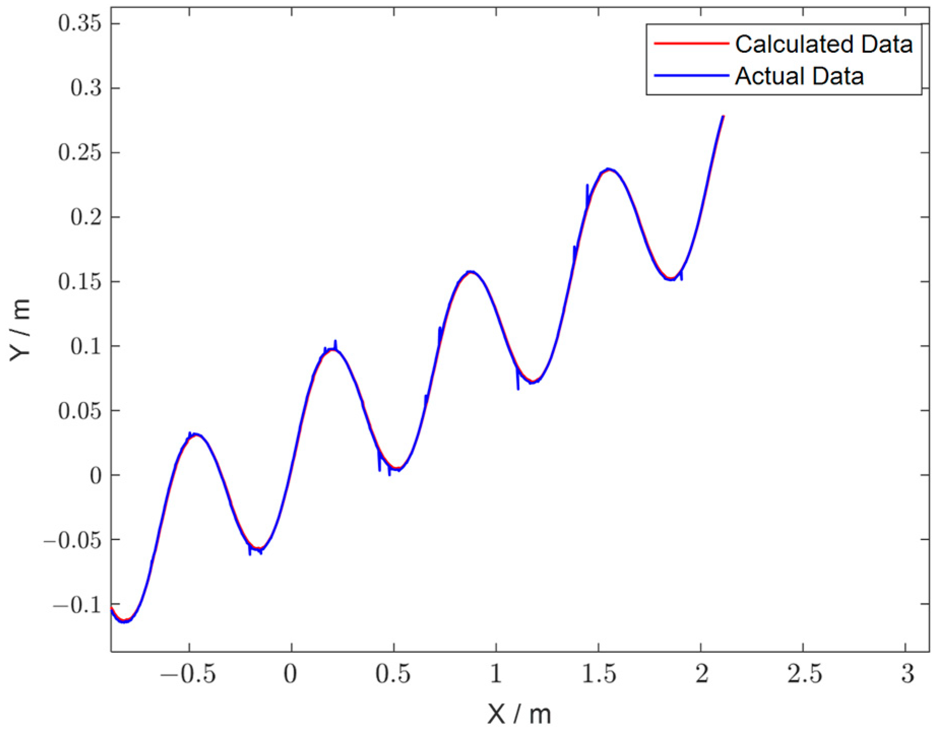
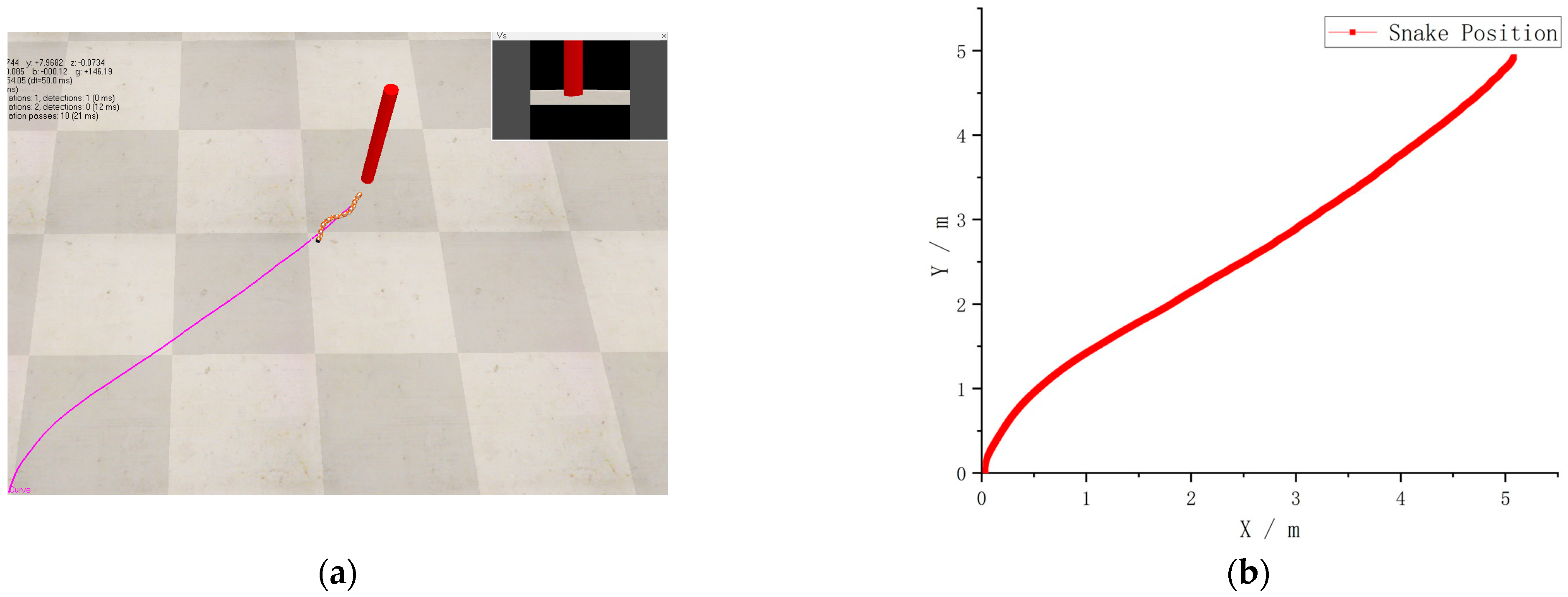
3.3. Double-Sine Serpentine Gait

Omega turn introduces a large number of parameters. as shown in Equation (14), which makes it more difficult to control the turning of a snake robot. Therefore, we conducted a lot of experiments on the above adjustable parameters, and found that the main parameters that determined the gait of the snake robot were a f , a t , k f , k t . This paper simplified the omega turn parameters, and adopted a double-sine serpentine gait by controlling yaw joint angle as:
ϕ n = a f sin ω t sin ω t + k f n + a t sin ω t sin ω t + k t n ,  
where ϕ n , ω ,   n , k f , k t , a f , a t have the same definitions as in Equations (13) and (14), the first part of Equation (15) controls forward movement of the snake robot, and the second part of Equation (15) controls the robot’s steering.
Each control parameter is the key factor to determine the motion form of the snake robot. The existing literature [10] explained the influence of gait control parameters A , k on the motion form of the snake robot. Parameters a f , k f have the same influence, which determines the wave amplitude of the snake robot, but they cannot change the direction of the robot movement. However, the qualitative relationship between the control parameter and the robot steering motion has not been explored by scholars. Therefore, the influence of the steering parameter a t ,   k t on the motion of a snake-like robot is worth discussing, which plays a vital role in the gait control of a snake robot.
First, we kept a t unchanged, and studied the influence of k t on the movement of the snake robot. We fixed a t = 30 ° , select k t = ± 10 ° , ± 20 ° ,   ± 90 ° in turn, then calculated the expected angle of each joint and inputted it into the snake model. The simulation results are shown in Figure 5. Experiments showed that when k t was small, the turning angle of the robot was not obvious and when k t = 90 ° , the turning angle was the largest. The effect of k t 0 ° , 180 ° was opposite to the effect of k t 180 ° , 0 ° on the turning direction.
Keeping k t constant, we studied the influence of a t on the movement of the snake robot. We fixed k t = 80 ° , and selected a t = ± 10 ° , ± 20 ° , ± 90 ° in sequence. The simulation results are shown in Figure 6. It was found that the larger a t was, the larger the turning angle was. The effect of a t 0 ° , 180 ° was opposite to the effect of a t 180 ° , 0 ° on the turning direction.
In summary, when a t changed very little, it could obviously change the direction of the snake robot. However, when k t changed very little, its influence on the turning motion of the robot was not obvious. It was found that a small change in the parameter a t could make the robot reach the desired direction angle. Therefore, in the subsequent control strategy, we only considered changing the control parameter a t to realize the turning of the snake robot.
Finally, we compared the double-sine serpentine gait with the traditional serpentine gait by controlling the snake robot to turn 60 ° , 90 °   and   120 ° , respectively. In each scenario, the control parameters that determined the forward direction were set as A = a f = 45 ° , K = k f = 55 ° , and temporal frequency ω = 40 ° . The results of the simulation experiments are shown in Figure 7, where the red dotted line represents the movement trajectory of the snake robot under the control of the double-sine serpentine gait, and the green solid line represents the movement trajectory under the control of the traditional serpentine gait.
It was found that the double-sine serpentine gait had a smaller turning radius than the traditional serpentine gait, making it more suitable for turning in narrow spaces. Counting the time spent by the two gaits when turning, as shown in Table 4, it was obvious that the double-sine serpentine gait took a short time to turn, which helped in quickly tracking the expected direction.

4. Controller Design

In order to realize target tracking of the snake robot, this paper designed a target tracking controller by combining double-sine serpentine gait and sliding mode control theory. The reasoning behind the design involved controlling the snake robot to track the desired direction angle with a new adaptive sliding mode controller, and pushing the snake robot forward with the double-sine serpentine gait function to reach the target point. The structure of the target tracking controller for the snake robot, based on double-sine serpentine gait, is shown in Figure 8.

4.1. Control Objectives

In this paper, we assumed that there was no obstacle. As shown in Figure 9, in order to achieve the target tracking task, it was only necessary to control the snake robot to track the expected path containing the target point. We supposed that the actual position and actual direction angle of the snake robot were set as p x , p y and θ ¯ . respectively, and the target position was set as x 0 , y 0 , and the expected direction angle recorded as θ ¯ e x p . Therefore, the control objective was that the position error e x = p x x 0 , e y = p y y 0 and direction angle error e θ ¯ = θ ¯ θ ¯ e x p all converged to the e x = 0 , e y = 0 , e θ ¯ = 0 limit cycle.
Since θ ¯ determines the forward direction, by controlling direction angle θ ¯ , the snake robot can move in the forward direction where the target point is located to quickly track the target point.
In order to accurately locate the target point, we established the quantitative relationship between the position error of the snake robot and its direction angle, which is shown in Equation (16):
θ ¯ e x p = arctan e y e x                   e x < 0 , arctan e y e x + π   e x > 0 .  
According to the analysis in Section 3, the double-sine serpentine gait can adjust the direction angle of the snake robot in a short time, which is conducive to making the snake robot quickly reach the desired direction. From the experiment in Section 3, it was found that the control parameters a t and k t could realize the steering of the robot. However, when the control parameter k t was small, the effect on the turning was not obvious. Therefore, we only considered controlling the parameter a t to achieve steering of the snake robot. There is a quantitative relationship between heading direction θ ¯ and the control parameter a t according to literature [33] which is as follows:
θ ¯ ˙ = b u t + d t = b a t t + d t ,  
where b is a constant related to the mechanical structure of the robot, d t is the external disturbance of the system, and a t is the joint controller input u t .

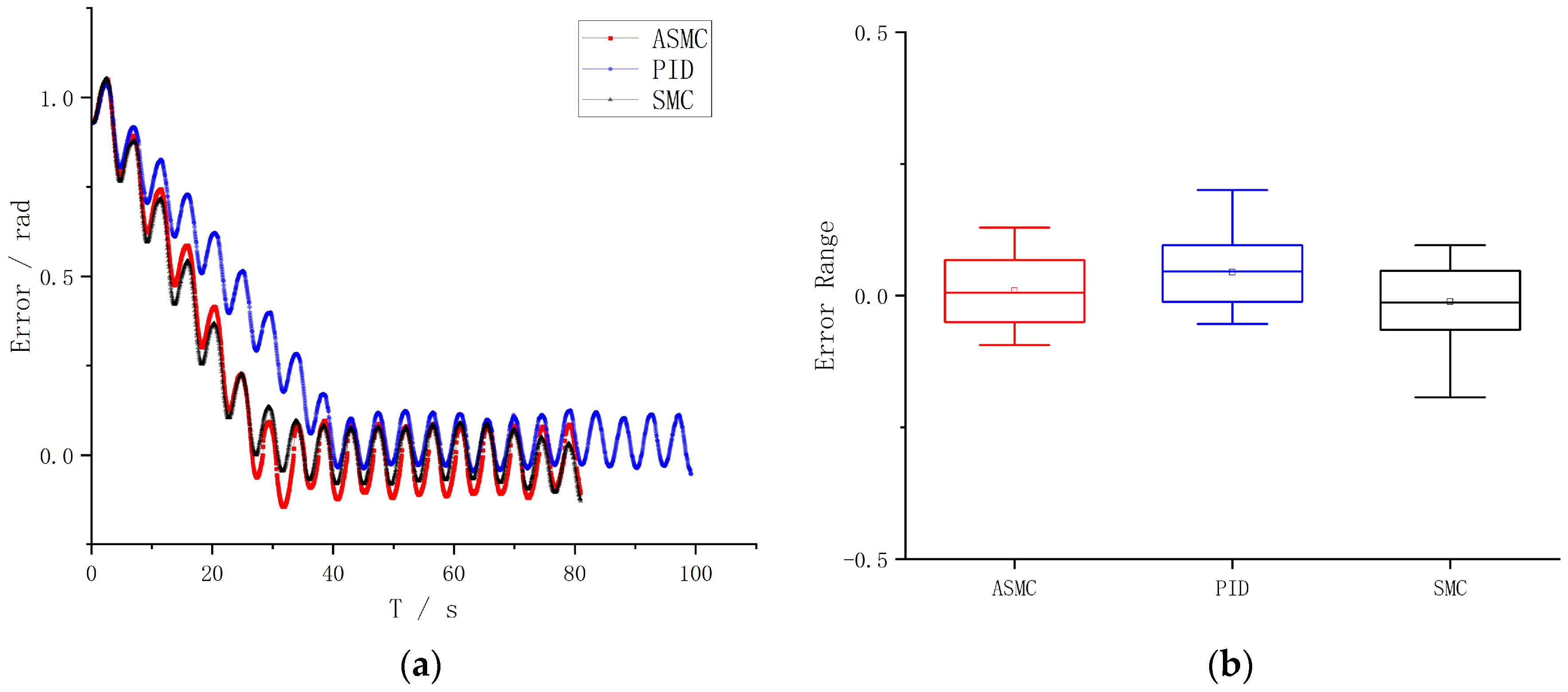
4.2. Sliding Mode Controller Design

Sliding mode control is a nonlinear control method that can force the system to follow the designed motion trajectory by purposefully changing the state of the system. Since the sliding mode is independent of object parameters and disturbances, SMC has the advantages of quick response speed and insensitive disturbance [40].
The sliding surface of the traditional sliding mode control method is shown in Equation (18). In order to reduce the steady state error of the control system, the integral term 0 t e d τ was introduced [40], as shown in Equation (19):
s t = c e t + e ˙ t .  
s t = c e t + e ˙ t + 0 t e d τ .
However, when the initial error was particularly large, adopting Equation (19) would cause the deterioration of the transient response, and even cause the system to be unstable. In order to improve the above situation, this paper replaced the integral term in Equation (19) with an appropriate potential energy function and selected the sliding surface of the snake robot control system as follows:
s t = c 1 e t + e ˙ t + c 2 0 t ψ e d τ .  
The tracking target error is e = θ ¯ θ ¯ e x p , and c 1 , c 2 + ,   ψ e is a nonlinear function [41], as shown in Equation (21):
ψ e = α s i n π e 2 α e < α , α                         e α , α                         e α .  
In the above equation, α + is an adjustable parameter. Figure 10 shows the function curve of ψ e when α = 3 . We found that when the absolute value of the error was e < α , ψ e > e and when the absolute value of the error was e α , ψ e e , it could be concluded that the error would be amplified when it was small, and saturated at ± α when it exceeded the design parameter α . The value ψ e could obtain the expected error state by designing the parameter α .
Considering that the snake robot system would be far away from the sliding surface, adopting the exponential reaching law could approach the sliding surface quickly, but the system shook violently when approaching the sliding surface. Although the jitter could be reduced by using the power reaching law, it took a long time to approach the sliding surface [42]. In order to improve the deficiencies of traditional reaching law, based on double power reaching law [43], this paper added an improved exponential approach term and designed the reaching law as follows:
s ˙ = ε 1 s a 1 s g n s ε 2 s a 2 s g n s k f s ,  
where ε 1 ,   ε 2 ,   k + , a 1 > 1 ,   0 < a 2 < 1 . f s is a nonlinear function, as shown in Equation (23), where q + .
f s = s                       s q , s g n s s > q .  
From Equations (20)–(23), the sliding mode control law could be designed as:
θ ¯ ˙ = c 1 1 c 2 ψ e + e ¨ t + ε ^ 1 s a 1 s g n s + ε ^ 2 s a 2 s g n s + k ^ f s + θ ¯ ˙ e x p t ,  
where ε ^ 1 , ε ^ 2 , k ^ is the estimated value of the reaching law parameters ε 1 ,   ε 2 ,   k , and the adaptive rate is shown in Equation (25).
ε ^ 1 ˙ = γ 1 s a 1 + 1 , ε ^ 2 ˙ = γ 2 s a 2 + 1 , k ^ ˙ = γ 3 s f s .  
In the above equation, γ 1 , γ 2 , γ 3 + are adaptive parameters.

4.3. Controller Stability Analysis

Select the Lyapunov function as follows:
V = 1 2 s 2 + 1 2 γ 1 ε ˜ 1 2 + 1 2 γ 2 ε ˜ 2 2 + 1 2 γ 3 k ˜ 2 ,  
where ε ˜ 1 = ε 1 ε ^ 1 , ε ˜ 2 = ε 2 ε ^ 2 , k ˜ = k k ^ represents the estimation error of ε 1 ,   ε 2 ,   k .
Combined with Equation (20), the above equation can be derived as follows:
V ˙ = s c 1 e ˙ + e ¨ + c 2 ψ e 1 γ 1 ε ˜ 1 ε ^ 1 ˙ 1 γ 2 ε ˜ 2 ε ^ 2 ˙ 1 γ 3 k ˜ k ^ ˙ = c 1 θ ¯ ˙ θ ¯ ˙ e x p + e ¨ + c 2 ψ e 1 γ 1 ε ˜ 1 ε ^ 1 ˙ 1 γ 2 ε ˜ 2 ε ^ 2 ˙ 1 γ 3 k ˜ k ^ ˙ .  
Putting Equation (24) into the above equation, we get:
V ˙ = ε ^ 1 s a 1 + 1 ε ^ 2 s a 2 + 1 k ^ s f s 1 γ 1 ε ˜ 1 ε ^ 1 ˙ 1 γ 2 ε ˜ 2 ε ^ 2 ˙ 1 γ 3 k ˜ k ^ ˙ .  
Combined with the adaptive rate Equation (25), we obtain:
V ˙ = ε ^ 1 s a 1 + 1 ε ^ 2 s a 2 + 1 k ^ s f s 1 γ 1 ε 1 ε ^ 1 ε ^ 1 ˙ 1 γ 2 ε 2 ε ^ 2 ε ^ 2 ˙           1 γ 3 k k ^ k ^ ˙ = ε ^ 1 s a 1 + 1 ε ^ 2 s a 2 + 1 k ^ s f s 1 γ 1 ε 1 ε ^ 1 γ 1 s a 1 + 1           1 γ 2 ε 2 ε ^ 2 γ 2 s a 2 + 1 1 γ 3 k k ^ γ 3 s f s = ε 1 s a 1 + 1 ε 2 s a 2 + 1 k s f s .  
For Equation (29), when s q , the above equation can be written as:
V ˙ = ε 1 s a 1 + 1 ε 2 s a 2 + 1 k s 2 0 .  
In the above equation, if and only if s = 0 , then   V ˙ = 0 .
Similarly, when s > q , Equation (29) can be written as:
V ˙ = ε 1 s a 1 + 1 ε 2 s a 2 + 1 k s 0 .  
In the above equation, if and only if s = 0 , then   V ˙ = 0 .
According to LaSalle’s invariance principle, when t , s 0 . If and only if   e = 0 , we have ψ e = 0 . If and only if e = 0 and e ˙ = 0 , we have s = 0 . From lim t s t = 0 , we can obtain lim t e t = lim t e ˙ t = 0 . When t , we have θ ¯ θ ¯ e x p 0 , and θ ¯ ˙ θ ¯ ˙ e x p 0 . Therefore, the error of the tracking control system eventually tends to zero. The controller that we designed is stable.

5. Simulation Results

In this part, we used the CoppeliaSim robot simulator software and MATLAB [39] to verify the effectiveness of the above control strategy. The initial position and the initial direction angle of the snake robot were set to 0 ,   0 and 90 ° , respectively. The target was set to a cylinder, and its position was 5 ,   5 . The initial state of the snake robot is shown in Figure 11.
The control parameters in the gait control function were set to a f = 30 ° ,   k f = 60 ° ,   k t = 90 ° ,   ω = 40 ° , and the initial value of a t was set to zero. The control parameters in the proposed adaptive sliding mode controller (ASMC) were set to c 1 = 150 , c 2 = 5 , a 1 = 1.1 , a 2 = 0.1 , q = 1 ,   α = 0.01 ,   γ 1 = 0.001 , γ 2 = 0.01 , γ 3 = 0.01 . The results of the simulation experiment are shown in Figure 12.
According to Figure 12a,b, the snake robot with the proposed control strategy could effectively reach the target. As shown in Figure 12c,d, the snake robot tracked the expected direction in about 30 s, and, finally, tracked the target in about 81 s. Note that since the direction angle of the snake robot was a sine wave affected by a serpentine gait, its direction angle error was also a sinusoidal waveform [27]. The closer the error was to zero, the better the tracking control effect would be.
In order to further explore the superiority of ASMC in the proposed control strategy, it was compared with a sliding mode controller (SMC) and a PD controller. The expressions and parameters of each controller were set as follows:
ASMC:
θ ¯ ˙ = c 1 1 ( c 2 ψ e + e ¨ t + ε ^ 1 s a 1 s g n s + ε ^ 2 s a 2 s g n s + k ^ f s ) + θ ¯ ˙ e x p t , where the parameter setting is the same as above.
PD controller:
θ ¯ ˙ = b 1 k p e + k d e ˙ , where b = 0.05 , k p = 1 ,   k d = 0.26 .
SMC:
θ ¯ ˙ = c 1 1 ε s a s g n s + e ¨ + c 2 e + θ ¯ ˙ e x p t . We adopt the power reaching law, and the sliding surface is s t = c e t + e ˙ t + 0 t e d τ . Set parameters c 1 = 300 , c 2 = 1 , ε = 100 , a = 0.55 .
To highlight the robustness and accuracy of the controllers in the process of tracking the desired target, we added external disturbance d t = 2 2 π e 2 t 5 in the experiments. The error of the direction angle with the above controllers is shown in Figure 13a, and the stabilized data of error, drawn as a box plot, is shown in Figure 13b.
According to Figure 13a, it can be seen that ASMC made the snake robot track the expected direction in 30 s, SMC made snake robot track the expected direction in 36 s, and PID made snake robot track the expected direction in 41 s. Compared with the PD controller and SMC, it was found that the proposed controller could quickly reduce the error and track the expected direction in a short time. Combined with Figure 13b, it could be seen that the error of ASMC was concentrated around 0.002 rad, the error of SMC was concentrated around −0.015 rad, and the error of PID was concentrated around 0.047 rad. Compared with the other two controllers, the state error of ASMC was more concentrated around 0. In brief, ASMC obviously converged faster than the other controllers in the case of external disturbance, and ASMC had higher tracking accuracy. Therefore, the tracking performance of ASMC was superior.
Finally, in order to verify the efficiency of the double-sine serpentine gait in our control strategy, we compared the result of the double-sine serpentine gait (see in Figure 12) with the result of regular gait [18] (see in Figure 14) for target tracking control. Figure 14 shows that the robot with regular gait tracked the expected direction in about 90 s, and tracked the target in about 160 s. Compared with the double-sine serpentine gait, the regular gait converged slower, and it took longer to reach the target point, which further verified that the double-sine serpentine gait in our control strategy helped ln quickly tracking the expected direction.

6. Conclusions

In this paper, an adaptive target tracking controller, based on the double-sine serpentine gait, was proposed. Considering traditional serpentine gait with its low movement efficiency, we established a double-sine serpentine gait, a superposition of two coplanar sine waves, which has a smaller turning radius and faster turning speed. After verification through simulation experiments, the double-sine serpentine gait was found to rapidly adjust the forward direction of the snake robot. Furthermore, an adaptive sliding mode controller was proposed in this paper to improve the robustness and convergence speed of the snake robot. Compared with a PD controller and SMC, the proposed controller enabled the snake robot to track the target point more quickly and accurately. However, the control strategy proposed in this paper was based on joint angle control which is only applicable to an ideal environment. In the future, considering robot motion with accuracy in the real environment, it is necessary to introduce joint torque control. This paper only studied target tracking control with no obstacles, so we need to further add an obstacle-avoiding strategy based to this control strategy. To improve the adaptability of the snake robot in complex environments, we will further explore the robust tracking of the snake robot on complex paths (including straight and curved paths) based on the research obtained in this paper.

Author Contributions

All authors contributed to this work. Conceptualization, Z.L. and W.W.; methodology, Z.L. and X.L.; software, Z.L. and S.H.; validation, Z.L. and W.W.; writing—original draft, Z.L.; writing—review and editing, Z.L., W.W., X.L. and S.H. All authors have read and agreed to the published version of the manuscript.

Funding

This work was supported by the National Natural Science Foundation of China [Grant Nos. 61573148, 61603358]; and the Science and Technology Planning Project of Guangdong Province, China [Grant Nos. 2015B010919007, 2019A050520001].

Institutional Review Board Statement

Not applicable.

Informed Consent Statement

Not applicable.

Data Availability Statement

The data that support the findings of this study are available on request from the corresponding author. The data are not publicly available due to privacy and ethical restrictions.

Conflicts of Interest

The authors declare no conflict of interest. The funders had no role in the design of the study; in the collection, analyses, or interpretation of data; in the writing of the manuscript, or in the decision to publish the results.

References

  1. Yang, X.; Zheng, L.; Lü, D.; Wang, J.; Wang, S.; Su, H.; Wang, Z.; Ren, L. The snake-inspired robots: A review. Assem. Autom. 2022, 42, 567–583. [Google Scholar] [CrossRef]
  2. Liu, Z.; Wang, Y.; Wang, J.; Fei, Y.; Du, Q. An obstacle-avoiding and stiffness-tunable modular bionic soft robot. Robotica 2020, 40, 2651–2665. [Google Scholar] [CrossRef]
  3. Li, D.; Deng, H.; Pan, Z.; Xiu, Y. Collaborative obstacle avoidance algorithm of multiple bionic snake robots in fluid based on IB-LBM. ISA Trans. 2022, 122, 271–280. [Google Scholar] [CrossRef] [PubMed]
  4. Chen, J.; Qiao, H. Muscle-synergies-based neuromuscular control for motion learning and generalization of a musculoskeletal system. IEEE Trans. Syst. Man Cybern. Syst. 2021, 51, 3993–4006. [Google Scholar] [CrossRef]
  5. Bhandari, G.; Raj, R.; Pathak, P.; Yang, J. Robust control of a planar snake robot based on interval type-2 Takagi–Sugeno fuzzy control using genetic algorithm. Eng. Appl. Artif. Intell. 2022, 116, 105437. [Google Scholar] [CrossRef]
  6. Jiang, X.; Yang, F.; Shi, S. Design and full-link trajectory tracking control of underwater snake robot with vector thrusters under strong time-varying disturbances. Ocean. Eng. 2022, 266, 113012. [Google Scholar] [CrossRef]
  7. Mahdi, H. Dynamics and computed-muscle-force control of a planar muscle-driven snake robot. Actuators 2022, 11, 194. [Google Scholar]
  8. Virgala, I.; Kelemen, M.; Prada, E.; Sukop, M.; Kot, T.; Bobovský, Z.; Varga, M.; Ferenčík, P. A snake robot for locomotion in a pipe using trapezium-like travelling wave. Mech. Mach. Theory 2021, 158, 104221. [Google Scholar] [CrossRef]
  9. Zhu, L.; Yang, P.; Li, F.; Wang, K.; Shui, L.; Chen, X. On the snake-like lateral un-dulatory locomotion in terrestrial, aquatic and sand environments. J. Mech. Phys. Solids 2021, 157, 104629. [Google Scholar] [CrossRef]
  10. Liu, X.; Lin, G.; Wei, W. Adaptive transition gait planning of snake robot based on polynomial interpolation method. Actuators 2022, 11, 222. [Google Scholar] [CrossRef]
  11. Bae, J.; Kim, M.; Song, B.; Yang, J.; Kim, D.; Jin, M.; Yun, D. Review of the latest research on snake robots focusing on the structure, motion and control method. Int. J. Control Autom. Syst. 2022, 20, 3393–3409. [Google Scholar] [CrossRef]
  12. Qin, G.; Wu, H.; Cheng, Y.; Pan, H.; Zhao, W.; Shi, S.; Song, Y.; Ji, A. Adaptive trajectory control of an under-actuated snake robot. Appl. Math. Model. 2022, 106, 756–769. [Google Scholar] [CrossRef]
  13. Han, S.; Chon, S.; Kim, J.; Seo, J.; Shin, D.G.; Park, S.; Kim, J.T.; Kim, J.; Jin, M.; Cho, J. Snake Robot Gripper Module for Search and Rescue in Narrow Spaces. IEEE Robot. Autom. Lett. 2022, 7, 1667–1673. [Google Scholar] [CrossRef]
  14. Baysal, Y.; Altas, I. Modelling and simulation of a wheel-less snake robot. In Proceedings of the 2020 7th International Conference on Electrical and Electronics Engineering (ICEEE), Antalya, Turkey, 14–16 April 2020; pp. 285–289. [Google Scholar]
  15. Huang, Z.; Ma, S.; Lin, Z.; Zhu, K.; Wang, P.; Ahmed, R.; Ren, C.; Marvi, H. Impact of caudal fin geometry on the swimming performance of a snake-like robot. Ocean. Eng. 2022, 245, 110372. [Google Scholar] [CrossRef]
  16. Gray, J. The mechanism of locomotion in snakes. J. Exp. Biol. 1946, 23, 101–120. [Google Scholar] [CrossRef] [PubMed]
  17. Mori, M.; Hirose, S. Locomotion of 3D snake-like robots–shifting and rolling control of active cord mechanism ACM-R3. J. Robot. Mechatron. 2006, 18, 521–528. [Google Scholar] [CrossRef]
  18. Hirose, S. Biologically Inspired Robots: Snake-Like Locomotors and Manipulators; Oxford University Press: London, UK, 1993. [Google Scholar]
  19. Ye, C.; Ma, S.; Li, B.; Wang, Y. Turning and side motion of snake-like robot. In Proceedings of the IEEE International Conference on Robotics and Automation, 2004. Proceedings. ICRA ’04. 2004, New Orleans, LA, USA, 26 April–1 May 2004; pp. 5075–5080. [Google Scholar]
  20. Ye, C.; Ma, S.; Li, B.; Wang, Y. Study on turning and sidewise motion of a snake-like robot. Chin. J. Mech. Eng. 2004, 40, 119–123, 128. [Google Scholar] [CrossRef]
  21. Dai, J.; Faraji, H.; Gong, C.; Hatton, R.; Goldman, D.; Choset, H. Geometric swimming on a granular surface. In Proceedings of the Robotics: Science and Systems 2016, Ann Arbor, MI, USA, 18–22 June 2016. [Google Scholar]
  22. Wang, T.; Chong, B.; Deng, Y.; Fu, R.; Choset, H.; Goldman, D. Generalized omega turn gait enables agile limbless robot turning in complex environments. In Proceedings of the 2022 International Conference on Robotics and Automation (ICRA), Philadelphia, PA, USA, 23–27 May 2022; pp. 1–7. [Google Scholar]
  23. Wang, T.; Chong, B.; Diaz, K.; Whitman, J.; Lu, H.; Travers, M.; Goldman, D.; Choset, H. The omega turn: A biologically-inspired turning strategy for elongated limbless robots. In Proceedings of the 2020 IEEE/RSJ International Conference on Intelligent Robots and Systems (IROS), Las Vegas, NV, USA, 24 October 2020–24 January 2021; pp. 7766–7771. [Google Scholar]
  24. Liu, X.; Onal, C.; Fu, J. Reinforcement learning of a CPG-regulated locomotion controller for a soft snake robot. arXiv 2022, arXiv:2207.04899. [Google Scholar]
  25. Takemori, T.; Tanaka, M.; Matsuno, F. Adaptive helical rolling of a snake robot to a straight pipe with irregular cross-sectional shape. IEEE Trans. Robot. 2022, 1–15. [Google Scholar] [CrossRef]
  26. Jiang, Z.; Otto, R.; Bing, Z.; Huang, K.; Knoll, A. Target tracking control of a wheel-less snake robot based on a supervised multi-layered SNN. In Proceedings of the 2020 IEEE/RSJ International Conference on Intelligent Robots and Systems (IROS), Las Vegas, NV, USA, 24 October 2020–24 January 2021; pp. 7124–7130. [Google Scholar]
  27. Liljebäck, P.; Pettersen, K.; Stavdahl, Ø.; Gravdahl, J.T. Snake Robots Modelling, Mechatronics, and Control; Springer Science & Business Media: Berlin/Heidelberg, Germany, 2012. [Google Scholar]
  28. Liljebäck, P.; Pettersen, K. Waypoint guidance control of snake robots. In Proceedings of the 2011 IEEE International Conference on Robotics and Automation, Shanghai, China, 9–13 May 2011; pp. 937–944. [Google Scholar]
  29. Kelasidi, E.; Liljebäck, P.; Pettersen, K.; Gravdahl, J. Integral line-of-sight guidance for path following control of underwater snake robots: Theory and experiments. IEEE Trans. Robot. 2017, 33, 610–628. [Google Scholar] [CrossRef] [Green Version]
  30. Ariizumi, R.; Takahashi, R.; Tanaka, M.; Asai, T. Head-trajectory-tracking control of a snake robot and its robustness under actuator failure. IEEE Trans. Control Syst. Technol. 2019, 27, 2589–2597. [Google Scholar] [CrossRef]
  31. Zhang, D.; Li, B.; Chang, J. Path following method for snake robot based on the angle symmetry adjustment. Robot 2019, 41, 788–794, 833. [Google Scholar]
  32. Zhang, D. A path tracking method for the snake robot based on the path edge guidance strategy. Robot 2021, 43, 36–43. [Google Scholar]
  33. Xiao, W. Design and Research of Advanced Gaits on Snake Robot. Master’s Thesis, South China University of Technology, Guangzhou, China, 2021. [Google Scholar]
  34. Cao, Z.; Zhang, D.; Zhou, M. Direction control and adaptive path following of 3-D snake-like robot motion. IEEE Trans. Cybern. 2022, 52, 10980–10987. [Google Scholar] [CrossRef]
  35. Wang, C.; Peng, Y.; Li, D.; Pan, Z.; Deng, H.; Li, D.; Li, B. Turning strategy of snake-like robot based on serpenoid curve under cloud assisted smart conditions. Clust. Comput. 2019, 22, 13041–13053. [Google Scholar] [CrossRef]
  36. Craig, J. Introduction to Robotics: Mechanics and Control, 4th ed.; China Machine Press: Beijing, China, 2018. [Google Scholar]
  37. Wei, W.; Li, Y.; Liao, Z.; Zhang, J. Kinematics modeling of snake-like robot based on screw theory. J. South China Univ. Technol. Nat. Sci. Ed. 2019, 47, 1–8. [Google Scholar]
  38. Wei, W.; Li, Y.; Gao, Y.; Xu, J. Safe climbing of snake-like robot based on screw and envelope theory. J. South China Univ. Technol. Nat. Sci. Ed. 2019, 47, 13–23. [Google Scholar]
  39. Tursynbek, I.; Shintemirov, A. Modeling and Simulation of Spherical Parallel Manipulators in CoppeliaSim (V-REP) Robot Simulator Software. In Proceedings of the 2020 International Conference Nonlinearity, Information and Robotics (NIR), Innopolis, Russia, 3–6 December 2020; pp. 1–6. [Google Scholar]
  40. Liu, J. Sliding Mode Control Design and Matlab Simulation: The Basic Theory and Design Method, 4th ed.; Tsinghua University Press: Beijing, China, 2019. [Google Scholar]
  41. Li, P.; Zheng, Z. Sliding mode control approach with nonlinear integrator. Control Theory Appl. 2011, 28, 421–426. [Google Scholar]
  42. Li, T. Nonlinear integral sliding mode control method based on new reaching law. Control Eng. China 2019, 26, 2031–2035. [Google Scholar]
  43. Yue, C.; Qian, L.; Chen, L.; Tian, L.; Yang, H. Adaptive control for artillery chain driving powder based on double power reaching law. J. Southeast Univ. Nat. Sci. Ed. 2017, 47, 1135–1140. [Google Scholar]
Figure 1. Simulation model of snake robot.
Actuators 12 00038 g001
Figure 2. Simple structure of snake robot with N 1 yaw joints.
Actuators 12 00038 g002
Figure 3. The screw coordinate model of snake robot.
Actuators 12 00038 g003
Figure 4. Comparison between calculated position and actual position of the robot tail.
Actuators 12 00038 g004
Figure 5. The influence of control parameter k t on the movement of snake robot.
Actuators 12 00038 g005
Figure 6. The influence of control parameter a t on the movement of snake robot.
Actuators 12 00038 g006
Figure 7. Comparison experiments of double-sine serpentine gait and traditional serpentine gait.
Actuators 12 00038 g007
Figure 8. The structure of target tracking controller.
Actuators 12 00038 g008
Figure 9. Schematic diagram of target tracking control of snake robot.
Actuators 12 00038 g009
Figure 10. The function curve of ψ e when α = 3 .
Actuators 12 00038 g010
Figure 11. The initial state of the snake robot.
Actuators 12 00038 g011
Figure 12. Simulation experiment results of target tracking control: (a) The trajectory of snake robot under tracking control; (b) Snake robot mass centric coordinates; (c) Desired direction angle and actual direction angle curve; (d) The error curve of the direction angle of snake robot.
Actuators 12 00038 g012aActuators 12 00038 g012b
Figure 13. Comparison of control error results of each controller: (a) The error curve of the direction angle; (b) Box plot of state error.
Actuators 12 00038 g013
Figure 14. Simulation results of target tracking based on regular gait.
Actuators 12 00038 g014
Table 1. Parameters that describe the snake robot.
SymbolDescriptionVector
N The total number of joints
n The joint index
l The length of a link
θ ¯ The forward direction angle of snake robot
θ ¯ e x p The expected direction angle of snake robot
θ n Angle between the link n and the global x -axis θ N + 1
ϕ n Angle of joint n ϕ N
r n The center point of joint n r N
ω n The unit vector in the direction of the rotation axis of joint n ω N
ξ n The twist of joint n ξ N
p x , p y Global coordinates of the center of mass of snake robot p 2
Table 2. Overview of snake robot specifications in simulation.
ItemsDescription
Mass1.5 kg
Length l s = 0.09   m ,   l = 0.07   m ,   l e = 0.10   m
Diameter0.05 m
SensingAngle sensor, Vision sensor, Proximity sensor
Number of modules17
Number of joints16
Connection mode between modulesOrthogonal connection
Table 3. Comparison of calculated data and actual data of pose matrix.
Pose MatrixCalculated DataActual Data
Time
2.20 s 0.0009 0.0697 0.9976 0.8325 0.0023 0.9976 0.0697 0.1103 1.0000 0.0023 0.0008 0.0534 0 0 0 1 0.0005 0.0696 0.9976 0.8368 0.0023 0.9976 0.0696 0.1117 1.0000 0.0023 0.0003 0.0534 0 0 0 1
3.70 s 0.0009 0.4387 0.8987 0.6972 0.0019 0.8986 0.4387 0.0973 1.0000 0.0021 0.0001 0.0534 0 0 0 1 0.0005 0.4386 0.8987 0.7012 0.0019 0.8987 0.4386 0.0991 1.0000 0.0020 0.0004 0.0534 0 0 0 1
12.95 s 0.0005 0.2357 0.9718 0.1946 0.0017 0.9718 0.2357 0.0506 1.0000 0.0015 0.0001 0.0534 0 0 0 1 0.0001 0.2357 0.9718 0.1988 0.0017 0.9718 0.2358 0.0507 1.0000 0.0017 0.0004 0.0534 0 0 0 1
29.75 s 0.0003 0.5652 0.8249 0.6715 0.0034 0.8249 0.5652 0.0911 1.0000 0.0027 0.0022 0.0534 0 0 0 1 0.0001 0.5651 0.8250 0.6675 0.0032 0.8249 0.5651 0.0900 1.0000 0.0027 0.0018 0.0534 0 0 0 1
50.05 s 0.0006 0.2771 0.9608 2.1352 0.0030 0.9608 0.2771 0.2896 1.0000 0.0027 0.0014 0.0534 0 0 0 1 0.0003 0.2770 0.9609 2.1309 0.0027 0.9609 0.2770 0.2895 0.9999 0.0025 0.0010 0.0534 0 0 0 1
Table 4. Comparison of turning time.
GaitDouble-Sine Serpentine GaitTraditional Serpentine Gait
Turning Time
60 ° Turning Time11.15 s39.55 s
90 ° Turning Time16.85 s52.95 s
120 ° Turning Time22.15 s89.70 s
Disclaimer/Publisher’s Note: The statements, opinions and data contained in all publications are solely those of the individual author(s) and contributor(s) and not of MDPI and/or the editor(s). MDPI and/or the editor(s) disclaim responsibility for any injury to people or property resulting from any ideas, methods, instructions or products referred to in the content.

