An Adaptive Dynamic Surface Technology-Based Electromechanical Actuator Fault-Tolerant Scheme for Blair Mine Hoist Wire Rope Tension Control System

Abstract

As an important equipment for deep well hoisting, the safe and stable operation of the Blair mine hoist is vital for the development and utilization of deep mineral resources. However, it is always a challenging task to keep consistent wire rope tension in the event of an actuator fault. In this study, an adaptive dynamic surface technology-based actuator fault-tolerant scheme is proposed. A fault observer with a neural network adaptation term is designed to estimate the loss of actuator efficiency caused by faults. Considering the redundant characteristic of the two actuators, a novel dynamic surface technology-based controller with a fuzzy assignment and state constraints is developed to eliminate the impact of fault. The stability of the closed-loop system under the proposed strategy is theoretically proved by rigorous Lyapunov analysis. Comparative experiments under various conditions are carried out on a xPC based mine hoist platform, and the results show the applicability together with the superiority of the proposed scheme.

1. Introduction

As the throat equipment connecting the underground and the ground of the ultra-thousand-meter-deep mine, the efficient and reliable operation of the Blair mine hoist is directly related to the life safety of the miners and the development of deep mineral resources. Although the safety level of the mine hoist has been continuously improved with the progress of research, safety risks still exist due to the harsh working environment of the equipment [1]. One of the important problems is that the wire rope tension of the mine hoist will fluctuate greatly under the action of multiple factors such as the partial load of the skip [2], the guide rail friction [3], and the inconsistent winding [4], which seriously affects the service life of the wire rope [5]. According to coal mine safety regulations in China, the difference between the tension of any hoisting wire rope and the average tension shall not exceed ±10%. Therefore, real-time measurement and control of the wire rope tension is necessary to ensure the safe operation of the hoist.

To prevent accidents, a wire rope tension control method has always received extensive attention from scholars. Wang et al. [6] presented a backstepping-based boundary control law to stabilize the mine hoist wire rope tension oscillation state. Zhu et al. [7] designed a nonlinear disturbance observer-based adaptive scheme to improve the performance of the wire rope tension coordination controller. In the literature [8], an intelligent learning control method is used to enhance the tension control effect. Li et al. [9] proposed an approach consisting of the disturbance observer and flatness-based controller to overcome the influence of system uncertainty on wire rope tension. By summing up the above research results, it can be found that nonlinear factors, including unknown disturbance [10], sensor delays [11], and model uncertainties [12], are the main consideration in the design process of the current tension coordination controllers. In addition, it should be pointed out that not only is the bounded interference quite important in engineering applications, but also handling the fault/failure in the system component is necessary for reliability [13]. Otherwise, the goal of tension coordination control cannot be achieved, and even a system crash can be caused. Fortunately, the fault-tolerant technique, which has been widely used in industrial equipment, such as the spacecraft [14], unmanned marine vehicles [15], battery assembly system [16], and robotic manipulators [17], provides a new direction for improving the reliability of the mine hoist closed-loop control system.

In general, fault-tolerant control systems can be classified into two main types: the passive fault-tolerant control system (PFTCS) and active fault-tolerant control system (AFTCS) [18,19]. For the PFTCS, controllers typically operate in offline mode under both normal and abnormal conditions, with predefined parameters to overcome the effects of faulty components. In [20], a novel passive fault-tolerant strategy made up of a Kalman filter and a sliding mode controller was applied to accomplish the path-following control of the electric vehicle under a steering system fault. A passive fault-tolerant switched state-feedback controller designed for linear multivariable systems with time-varying actuator faults was proposed in [21]. A weighted tube model predictive scheme-based passive fault-tolerant controller was developed in [22] to deal with an actuator efficiency loss fault of hypersonic vehicles. In [23], a hybrid fault-tolerant control strategy consisted of a Takagi-Sugeno fuzzy model, and a sliding mode control scheme was proposed to handle unmanned marine vehicles’ dynamic positioning problem in the case of a time-varying delay and thruster faults. An adaptive second-order fault-tolerant sliding mode controller with a proportional-integral-differential sliding surface was designed in [24] to achieve the speed control of an electromechanical system under a structural damage fault condition. As for the AFTCS, an online detection subsystem provides fault conditions constantly, which will guide the supervisory subsystem to adjust the structure and parameters of the controller to cut down faults’ effect on the whole system [25,26]. In [27], a DK-iteration approach-based multi-controller switching strategy was proposed to achieve an active fault-tolerant purpose for unmanned aerial vehicles. A novel AFTC consisting of an artificial neural-network-based fault detection and isolation subsystem and a nonlinear dynamic inversion controller with a new feedback structure for flight was presented in [28]. In [29], the design problem of the actuator fault-tolerant control for a class of two coupling permanent magnet synchronous motors system was discussed. An adaptive robust observer was built to estimate the actuator faults. An improved third-order sliding mode observer was developed in [30] for robot manipulator systems to heighten the effect of the nonsingular fast terminal sliding mode-based fault-tolerant controller. In [31], a dynamic proportional-integral observer-based nonlinear fault-tolerant controller was put forward to stabilize a nonlinear system with a partially unknown dynamic. A neuroadaptive observer and command filtered technique-based fault-tolerant controller was applied to overcome the position tracking problem for induction motors with possible actuator faults and load disturbances [32]. In [33], nonlinear disturbance observers, an asymmetric barrier Lyapunov function, and an adaptive compensation technique were combined to deal with the partial loss of effectiveness problem of the electro-hydraulic actuator system. An iterative learning algorithm-based fault-tolerant controller was established for repetitive systems with Brownian motion in [34]. To our best knowledge of relevant research, there are few existing works taking the fault-tolerant control problem of the mine hoist into account. In fact, electromechanical actuator failure will increase the risk of system oscillation as large flexible wire ropes are used in the mine hoist to carry the skip, which makes a fault-tolerant design of the tension coordination control system of critical importance [35]. On the other hand, the existing fault-tolerant schemes designed for other equipment, such as the H_∞ technique [36], sliding mode approach [37,38], adaptive method [39,40], model predictive control scheme [41], etc., are very difficult to be applied on the tension coordination control system without modifications owing to its special nonlinear structure.

Motivated by the above research, in this work, the wire rope tension coordination control problem for the mine hoist in the presence of actuator faults is considered. To achieve efficient actuator fault detection, a neural-network-based adaptive observer is designed and constructed. The controller thus can obtain more efficient fault information. In order to drive the wire rope tension difference into the allowable range under an actuator fault condition, an adaptive dynamic surface technology-based fault-tolerant control scheme is devised. In the control scheme, taking into account the redundant characteristic of the actuators, fuzzy rules are used to construct the control variable allocation factor. Furthermore, to improve control performance, the barrier function-based control law is proposed. The presented controller can not only realize coordination control of wire rope tension under normal working conditions but also maintain acceptable performance under an actuator fault condition. The main contributions of this paper can be summarized as: (1) Considering the Blair mine hoist wire rope tension control system with unknown disturbances, modelling errors and actuator faults, a novel adaptive dynamic surface technology-based fault-tolerant controller with a fuzzy assignment and state constraints, instead of the traditional dynamic surface controller design method, is developed, and the stability of the proposed strategy is mathematically proved; (2) The proposed design does not need to distinguish the type and specific location of actuator failures accurately, and determines the real-time reallocation of actuators with the fuzzy efficiency loss function. This helps to realize fault-tolerant control quickly, even if one side of the actuator is completely stuck which is a challenge for other controllers; and (3) The effectiveness of the proposed controller is verified by the experiments’ results. Unlike existing studies, relevant theories proposed in this paper are proved feasible in the experimental environment, which has strong engineering guiding significance.

This paper is organized as follows: Section 2 provides the nonlinear equation of the wire rope tension coordination control system with an actuator fault. In Section 3, the design of the proposed fault observer and fault-tolerant controller is illustrated. Besides, the stability proof of the overall closed-loop control system is proposed. In Section 4, the experimental design and results’ analysis are presented and discussed. Conclusions are given in Section 5.

2. Mathematical Model of Blair Mine Hoist

2.1. Wire Rope Tension Control Model

A typical Blair mine hoist with an electric cylinder tension adjustment device is shown in Figure 1. It can be seen that under the winding action of the drum, the skip is driven up or down by the vertical rope to realize the transportation of coal. Obviously, if the length difference appears between the left side of the wire rope and the right side, it is easy to cause overloading of one side of the wire rope as the skip withstands the constraint of the guide rail, which is the root cause of the requirement of tension coordination control. At this time, the active adjustment actuator is installed under the headgear sheave to compensate the rope length difference. For the design of the actuator, there are two forms, the hydraulic drive or electric drive. This paper selects the electric drive form for research.

As shown in Figure 2, the mine hoist dynamic model can be divided into three sub-models: the hoisting subsystem model, skip subsystem model, and electric drive actuator model.

In the actual operating conditions, the dynamic behaviors of the mine hoist caused by the interaction between the drum, the wire rope, and the headgear sheave are very complex [42]. Considering the complexity, accuracy, and calculation amount of the control model, the following assumptions are made: (1) The structure of the wire rope is simplified as an elastic wire with a distributed mass; (2) The elastic modulus of the catenaries and the vertical ropes is constant along its entire length; that is, its deformation characteristics conform to Hooke’s law; (3) Compared with the length of the vertical ropes, the lateral displacement of the ends of the vertical ropes on both sides is very small, and the lateral inclination angle of the vertical ropes on both sides can be ignored. Choose the state vector of the hoisting subsystem as

$${\mathit{x}}_{hs}={\left[\begin{array}{lllllll}{\theta }_{wd}\hfill & {\theta }_s^{\left(1\right)}\hfill & {\theta }_s^{\left(2\right)}\hfill & d_s^{\left(1\right)}\hfill & d_s^{\left(2\right)}\hfill & d_{cn}^{\left(1\right)}\hfill & d_{cn}^{\left(2\right)}\hfill \end{array}\right]}^{\mathrm{T}}$$

(1)

where ${\theta }_{wd}$ is rotation angle of the drum; ${\theta }_s^{\left(1\right)}$ and ${\theta }_s^{\left(2\right)}$ represent the rotation angle of the left and right headgear sheave, respectively. $d_s^{\left(1\right)}$ and $d_s^{\left(2\right)}$ denote the vertical displacement of the left and right headgear sheave. $d_{cn}^{\left(1\right)}$ and $d_{cn}^{\left(2\right)}$ indicate displacement of the end of the left and right vertical rope.

According to the above assumption, the displacement of any point on the catenary can be expressed as

$$x_{yc}^{\left(i\right)}={\theta }_s^{\left(i\right)}{r}_s^{\left(i\right)}-d_s^{\left(i\right)}\sin {\theta }_{qx}^{\left(i\right)}+\left(l_c^{\left(i\right)}-y_c^{\left(i\right)}\right){\left(l_c^{\left(i\right)}\right)}^{-1}\cdot \left({\theta }_{wd}{r}_{wd}^{\left(i\right)}-{\theta }_s^{\left(i\right)}{r}_s^{\left(i\right)}+d_s^{\left(i\right)}\sin {\theta }_{qx}^{\left(i\right)}\right)$$

(2)

where $r_{wd}^{\left(1\right)}$ and $r_{wd}^{\left(2\right)}$ denote the radius of the left and right part of the drum. The radii of the left and right headgear sheave are represented by $r_s^{\left(1\right)}$ and $r_s^{\left(2\right)}$. The inclination angles of the left and right catenary are denoted by ${\theta }_{qx}^{\left(1\right)}$ and ${\theta }_{qx}^{\left(2\right)}$. The real-time lengths of the left and right catenary are $l_c^{\left(1\right)}$ and $l_c^{\left(2\right)}$. For the point on the left catenary, $y_c^{\left(1\right)}$ indicates the displacement between the point and the left rope release point (C point). In addition, for the point on the right catenary, $y_c^{\left(2\right)}$ denotes the displacement between the point and the right rope release point (D point).

The displacement of any point on the vertical rope can be represented as

$$x_{yv}^{\left(i\right)}=d_{cn}^{\left(i\right)}+\left(l_v^{\left(i\right)}-y_v^{\left(i\right)}\right){\left(l_v^{\left(i\right)}\right)}^{-1}\cdot \left({\theta }_s^{\left(i\right)}{r}_s^{\left(i\right)}+d_s^{\left(i\right)}-d_{cn}^{\left(i\right)}\right)$$

(3)

where the real-time length of the left and right vertical rope are $l_v^{\left(1\right)}$ and $l_v^{\left(2\right)}$. For the point on the left vertical rope, $y_v^{\left(1\right)}$ is the displacement between the point and the upper point (A point) of the vertical rope. In addition, for the point on the right vertical rope, $y_v^{\left(2\right)}$ represents the displacement between the point and the right rope release point (B point).

Analyze the kinetic, potential, and dissipation energy of the hoisting subsystem; Appendix A presents the detailed calculation process, and then the nonlinear dynamic model of the hoisting subsystem can be represented as

$$\begin{array}{l}\frac{{\rho }_{wr}{l}_c^{\left(i\right)}{r}_s^{\left(i\right)}{r}_{wd}^{\left(i\right)}}{6}{\ddot{\theta }}_{wd}+\left[J_s^{\left(i\right)}+\frac{{\rho }_{wr}{\left(r_s^{\left(i\right)}\right)}^2\left(l_c^{\left(i\right)}+l_v^{\left(i\right)}\right)}{3}\right]{\ddot{\theta }}_s^{\left(i\right)}-k_v^{\left(i\right)}{r}_s^{\left(i\right)}{d}_{cn}^{\left(i\right)}\\ +\frac{{\rho }_{wr}{l}_v^{\left(i\right)}{r}_s^{\left(i\right)}}{6}{\ddot{d}}_{cn}^{\left(i\right)}-c_c^{\left(i\right)}{r}_s^{\left(i\right)}{r}_{wd}^{\left(i\right)}{\dot{\theta }}_{wd}+\left(c_c^{\left(i\right)}+c_v^{\left(i\right)}\right){\left(r_s^{\left(i\right)}\right)}^2{\dot{\theta }}_s^{\left(i\right)}+\left(c_v^{\left(i\right)}-c_c^{\left(i\right)}\sin {\theta }_{qx}^{\left(i\right)}\right)r_s^{\left(i\right)}{\dot{d}}_s^{\left(i\right)}\\ -c_v^{\left(i\right)}{r}_s^{\left(i\right)}{\dot{d}}_{cn}^{\left(i\right)}-k_c^{\left(i\right)}{r}_s^{\left(i\right)}{r}_{wd}^{\left(i\right)}{\theta }_{wd}+\left(k_c^{\left(i\right)}+k_v^{\left(i\right)}\right){\left(r_s^{\left(i\right)}\right)}^2{\theta }_s^{\left(i\right)}+\left(k_v^{\left(i\right)}-k_c^{\left(i\right)}\sin {\theta }_{qx}^{\left(i\right)}\right)r_s^{\left(i\right)}{d}_s^{\left(i\right)}\\ +\left(\frac{{\rho }_{wr}{l}_v^{\left(i\right)}{r}_s^{\left(i\right)}}{3}-\frac{{\rho }_{wr}{l}_c^{\left(i\right)}{r}_s^{\left(i\right)}}{3}\sin {\theta }_{qx}^{\left(i\right)}\right){\ddot{d}}_s^{\left(i\right)}=\frac{{\rho }_{wr}g{l}_c^{\left(i\right)}{r}_s^{\left(i\right)}\sin {\theta }_{qx}^{\left(i\right)}}{2}-\frac{{\rho }_{wr}g{l}_v^{\left(i\right)}{r}_s^{\left(i\right)}}{2}\end{array}$$

(4)

$$\begin{array}{l}-\frac{{\rho }_{wr}{l}_c^{\left(i\right)}{r}_{wd}^{\left(i\right)}\sin {\theta }_{qx}^{\left(i\right)}}{6}{\ddot{\theta }}_{wd}+\left(\frac{{\rho }_{wr}{l}_v^{\left(i\right)}{r}_s^{\left(i\right)}}{3}-\frac{{\rho }_{wr}{l}_c^{\left(i\right)}{r}_s^{\left(i\right)}}{3}\sin {\theta }_{qx}^{\left(i\right)}\right){\ddot{\theta }}_s^{\left(i\right)}+\frac{{\rho }_{wr}{l}_v^{\left(i\right)}}{6}{\ddot{d}}_{cn}^{\left(i\right)}\\ +\left(m_s^{\left(i\right)}+\frac{{\rho }_{wr}{l}_v^{\left(i\right)}}{3}+\frac{{\rho }_{wr}{l}_c^{\left(i\right)}}{3}{\sin }^2{\theta }_{qx}^{\left(i\right)}\right){\ddot{d}}_s^{\left(i\right)}+c_c^{\left(i\right)}{r}_{wd}^{\left(i\right)}\sin {\theta }_{qx}^{\left(i\right)}{\dot{\theta }}_{wd}+\left(c_v^{\left(i\right)}-c_c^{\left(i\right)}\sin {\theta }_{qx}^{\left(i\right)}\right)r_s^{\left(i\right)}{\dot{\theta }}_s^{\left(i\right)}\\ +\left(c_v^{\left(i\right)}+c_c^{\left(i\right)}{\sin }^2{\theta }_{qx}^{\left(i\right)}\right){\dot{d}}_s^{\left(i\right)}-c_v^{\left(i\right)}{\dot{d}}_{cn}^{\left(i\right)}+k_c^{\left(i\right)}{r}_{wd}^{\left(i\right)}\sin {\theta }_{qx}^{\left(i\right)}{\theta }_{wd}+\left(k_v^{\left(i\right)}-k_c^{\left(i\right)}\sin {\theta }_{qx}^{\left(i\right)}\right)r_s^{\left(i\right)}{\theta }_s^{\left(i\right)}\\ +\left(k_v^{\left(i\right)}+k_c^{\left(i\right)}{\sin }^2{\theta }_{qx}^{\left(i\right)}\right)d_s^{\left(i\right)}-k_v^{\left(i\right)}{d}_{cn}^{\left(i\right)}=F_{ema}^{\left(i\right)}-\frac{{\rho }_{wr}g{l}_v^{\left(i\right)}}{2}-m_s^{\left(i\right)}g-\frac{{\rho }_{wr}g{l}_c^{\left(i\right)}{r}_s^{\left(i\right)}}{2}\sin {\theta }_{qx}^{\left(i\right)}\end{array}$$

(5)

$$\begin{array}{l}\frac{{\rho }_{wr}{l}_v^{\left(i\right)}{r}_s^{\left(i\right)}}{6}{\ddot{\theta }}_s^{\left(i\right)}+\frac{{\rho }_{wr}{l}_v^{\left(i\right)}}{6}{\ddot{d}}_s^{\left(i\right)}+\left(m_{cn}^{\left(i\right)}+\frac{{\rho }_{wr}{l}_v^{\left(i\right)}}{3}\right){\ddot{d}}_{cn}^{\left(i\right)}-c_v^{\left(i\right)}{r}_s^{\left(i\right)}{\dot{\theta }}_s^{\left(i\right)}-c_v^{\left(i\right)}{\dot{d}}_s^{\left(i\right)}+c_v^{\left(i\right)}{\dot{d}}_{cn}^{\left(i\right)}\\ -k_v^{\left(i\right)}{r}_s^{\left(i\right)}{\theta }_s^{\left(i\right)}-k_v^{\left(i\right)}{d}_s^{\left(i\right)}+k_v^{\left(i\right)}{d}_{cn}^{\left(i\right)}=-F_{cn}^{\left(i\right)}-m_{cn}^{\left(i\right)}g-\frac{{\rho }_{wr}g{l}_v^{\left(i\right)}}{2}\end{array}$$

(6)

where ${\rho }_{wr}$ indicates the linear density of the wire ropes. $J_s^{\left(1\right)}$ and $J_s^{\left(2\right)}$ represent the equivalent moment of inertia of the left and right headgear sheave, respectively. $k_v^{\left(1\right)}=EA/l_v^{\left(1\right)}$ and $k_v^{\left(2\right)}=EA/l_v^{\left(2\right)}$ denote the stiffness coefficients of the left vertical rope and the right vertical rope which are a function of the rope length. EA is the stiffness constant. The stiffness coefficients of the left catenary and the right catenary are represented by $k_c^{\left(1\right)}=EA/l_c^{\left(1\right)}$ and $k_c^{\left(2\right)}=EA/l_c^{\left(2\right)}$.

Permanent magnet synchronous motors are used to drive the actuator action; the simplified equation of the motor can be represented as

$$\{\begin{array}{c}{u}_{mtd}^{(i)}=R_{mo}^{(i)}{i}_{mtd}^{(i)}+L_{mtd}^{(i)}\frac{d}{dt}{i}_{mtd}^{(i)}-{\omega }_e^{(i)}{L}_{mtq}^{(i)}{i}_{mtq}^{(i)}\\ u_{mtq}^{(i)}=R_{mo}^{(i)}{i}_{mtq}^{(i)}+L_{mtq}^{(i)}\frac{d}{dt}{i}_{mtq}^{(i)}+{\omega }_e^{(i)}\left(L_{mtd}^{(i)}{i}_{mtd}^{(i)}+{\psi }_{mtf}^{(i)}\right)\\ J_{hs}^{(i)}\hspace{0.17em}{\ddot{\theta }}_{hs}^{(i)}={\mathrm{T}}_{mt}^{(i)}\hspace{0.17em}-B_{hs}^{(i)}\hspace{0.17em}{\dot{\theta }}_{hs}^{(i)}-{\mathrm{T}}_{hs}^{(i)}\end{array}\begin{array}{cc}& \end{array}(i=1,2)$$

(7)

where ${\theta }_{hs}^{(1)}$ and ${\theta }_{hs}^{(2)}$ denote the rotation angles of the left and right actuator-driven motor, respectively. $J_{hs}^{(1)}$ and $J_{hs}^{(2)}$ indicate the equivalent moments of inertia of the left and right actuator-driven motor. $B_{hs}^{(1)}$ and $B_{hs}^{(2)}$ represent the damping coefficients of the left and right actuator-driven motor. ${\mathrm{T}}_{mt}^{(1)}$ and ${\mathrm{T}}_{mt}^{(2)}$ are the electromagnetic torque values of the left and right actuator-driven motor and can be defined as

$${\mathrm{T}}_{mt}^{(i)}=1.5\begin{array}{cc}{p}_{mt}^{(i)}\hspace{0.17em}{i}_{mtq}^{(i)}\left[i_{mtd}^{(i)}\left(L_{mtd}^{(i)}-L_{mtq}^{(i)}\right)+{\psi }_{mtf}^{(i)}\right]=& 1.5p_{mt}^{(i)}\end{array}{i}_{mtq}^{(i)}{\psi }_{mtf}^{(i)}\begin{array}{cc}+{\chi }_{mt}^{(i)}& \end{array}(i=1,2)$$

(8)

where $p_{mt}^{(1)}$ and $p_{mt}^{(2)}$ indicate the numbers of the left and right actuator-driven motor pole pair, respectively. $i_{mtq}^{(1)}$ and $i_{mtq}^{(2)}$ represent the currents of the left and right actuator-driven motor along q axes. $i_{mtd}^{(1)}$ and $i_{mtd}^{(2)}$ denote the currents of the left and right actuator-driven motor along d axes. $L_{mtd}^{(1)}$ and $L_{mtd}^{(2)}$ are the inductances of the left and right actuator-driven motor along d axes. The inductances of the left and right actuator-driven motor along q axes are represented by $L_{mtq}^{(1)}$ and $L_{mtq}^{(2)}$, respectively. ${\psi }_{mtf}^{(1)}$ and ${\psi }_{mtf}^{(2)}$ denote the flux linkage coefficients of the left and right actuator-driven motor. As the selected motors are generally the surface-mount type, thus, $L_{mtd}^{(i)}\approx L_{mtq}^{(i)}$ and the nonlinear term in Equation (8) satisfies ${\chi }_{mt}^{(i)}\approx 0$.

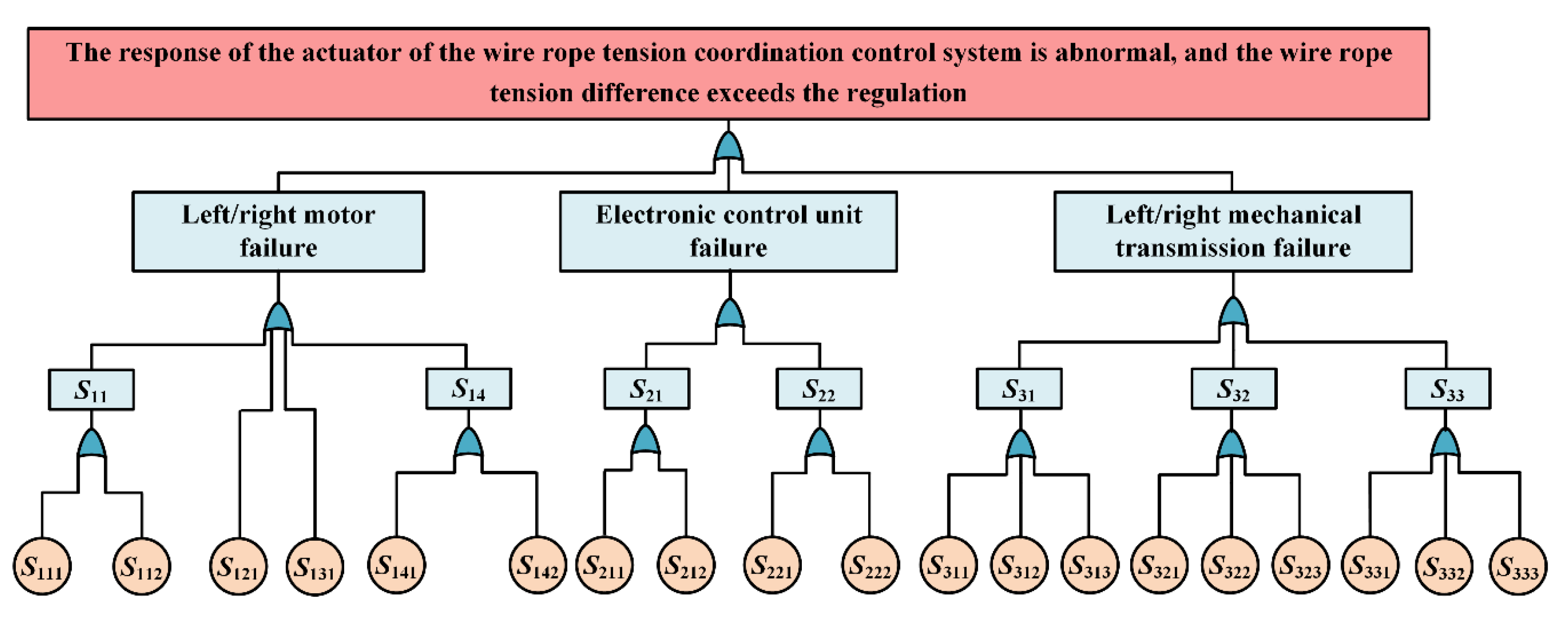
2.2. Problem Formulation of Actuator Fault

During the long-term service of the mine hoist wire rope tension control system, from the structure of the electric actuator, it can be known that key components such as the motor, gearbox, and screw mechanism may turn out faults [43,44]. The fault tree of electromechanical actuators in the tension coordination control system is shown in Figure 3. The failure event and the corresponding ID are shown in

Table 1. Electromechanical Actuator Failure Event and the Corresponding ID.

Event ID	Event	Event ID	Event
S11	Motor Winding Failure	S222	Board Circuit Failure
S111	Winding Short Circuit	S31	Gear Failure
S112	Winding Open Circuit	S311	Gear Surface Wear
S121	Rotor Eccentricity	S312	Gear Teeth Broken
S131	Unstable Supply Voltage	S313	Gear Teeth Deformation
S14	Motor Sensor Failure	S32	Bearing Failure
S141	Encoder Failure	S321	Structure Plastic Deformation
S142	Current Sensor Failure	S322	Surface Cracking and Spalling
S21	Cable Failure	S323	Surface Corrosion
S211	Cable Open Circuit	S33	Screw Mechanism Failure
S212	Cable Short Circuit	S331	Guide Wear
S22	Control Board Failure	S332	Screw Wear
S221	Board Loose	S333	Screw Deformation

. It is not difficult to know that each abnormal situation may correspond to a variety of component failures; for instance, electrical failure, structural deformation, and excessive frictional resistance may cause the actuator to be stuck. In addition, with the development of the same type of component failure to different extents, it will lead to different abnormal response situations. For example, in the early stage of screw deformation, the electromechanical actuator may show a response situation with reduced efficiency. When the bending deformation of the screw is large, the actuator will show a stuck response situation.

From a macro perspective, the abnormal response of the actuator subsystem of the tension coordination control system mainly includes several types, such as stuck situations, out-of-control situations, efficiency reduction, random fluctuation, and is reflected in the deviation between the actual output response and the expected response [45,46]. More specifically, the expected electromechanical actuator position refers to the action of the non-faulty actuator under a given input voltage, and the actual electromechanical actuator position refers to the action of the faulty actuator under the given input voltage. From the actual situation, for the electromechanical actuator, the movement resistance anomaly caused by mechanical deformation faults is defined as $f_{af1}^{\left(i\right)}$, the unstable control voltage of the motor due to an electronic unit failure as $f_{af2}^{\left(i\right)}$, and the transmission coefficient change as $f_{af3}^{\left(i\right)}$, and then the mathematical model of the electromechanical actuator with faults can be expressed as

$$\hspace{0.17em}\{\begin{array}{l}{J}_{hs}^{(i)}\hspace{0.17em}{\ddot{\theta }}_{hs}^{(i)}=1.5p_{mt}^{(i)}(\hspace{0.17em}{i}_{mtq}^{(i)}+f_{af2}^{\left(i\right)}){\psi }_{mtf}^{(i)}-B_{hs}^{(i)}\hspace{0.17em}{\dot{\theta }}_{hs}^{(i)}-{\mathrm{T}}_{hs}^{(i)}-f_{af1}^{\left(i\right)}\hfill \\ {\dot{d}}_{ema}^{(i)}=f_{af3}^{\left(i\right)}{z}_{bc}^{(i)}{z}_{gb}^{(i)}{\dot{\theta }}_{hs}^{(i)}\hfill \\ F_{ema}^{(i)}={\mathrm{T}}_{hs}^{(i)}/f_{af3}^{\left(i\right)}{z}_{bc}^{(i)}{z}_{gb}^{(i)}\hfill \end{array}\begin{array}{cc}& \end{array}(i=1,2)$$

(9)

where $z_{bc}^{\left(i\right)}$ and $z_{gb}^{\left(i\right)}$ indicate the transmission ration of the screw i and the gearbox i, respectively.

3. Adaptive Actuator Fault-Tolerant Controller Design

In this section, the dynamic surface technique-based adaptive fault-tolerant scheme will be developed for the wire rope tension control system’s actuator fault. The overall architecture of the control system is shown in Figure 4. In this approach, in light of the fact that the faulty actuator is unknown, adaptive actuator fault observers consisting of the left fault observer and right fault observer are firstly designed for the left actuator and the right actuator, respectively, which are applied to provide actuators’ fault information timely. Through the received fault indicators ${\Delta }_{fault}^{(i)}$ and sensor feedback information, utilizing the redundancy properties of the two actuators, the tension coordination control loop, which is the first design step of the controller for adaptive control distribution, and the actuator control loop, which is the second design step of the controller for fast reference tracking, are put forward. In this way, the electromechanical actuator can continue to drive the headgear sheave to run up and down under fault and disturbance conditions finally to achieve the control goal.

3.1. The Adaptive Actuator Fault Observer

For the actual fault detection system and control system, accurate estimation of the specific fault type and amplitude requires a large number of sensor signals, field data, and complex calculation processes, which is not conducive to the timely response and action of the control system. Therefore, for safety reasons, it is more meaningful to detect the abnormal response state and degree of the actuator in time for the actual system.

In this section, a fault observer is designed separately for each motor of electromechanical actuator. Combining the faults of the same channel in Equation (9), the state equation of i-th electromechanical actuator motor can be rewritten as

$$\{\begin{array}{l}{\dot{z}}_{fo}^{(i)}=m_{fo}^{(i)}{z}_{fo}^{(i)}+h_{fo}^{(i)}{u}_{fo}^{(i)}+G_{fo}^{(i)}+{\mathsf{\beta }}_{fo}^{(i)}\left(z_{fo}^{(i)}\right)\hfill \\ y_{fo}^{(i)}=C_{fo}{z}_{fo}^{(i)}\hfill \end{array}$$

(10)

where $z_{fo}^{(i)}={\left[\begin{array}{cc}{z}_{fo1}^{\left(i\right)}& z_{fo2}^{\left(i\right)}\end{array}\right]}^{\mathrm{T}}={\left[\begin{array}{cc}{\theta }_{hs}^{\left(i\right)}& {\dot{\theta }}_{hs}^{\left(i\right)}\end{array}\right]}^{\mathrm{T}}$ (i = 1,2) represent the i-th electromechanical actuator state variables. T represents the standard matrix transposition operation. $m_{fo}^{(i)}\left(z_{fo}^{(i)}\right)=\left[\begin{array}{cc}0& 1\\ 0& -B_{hs}^{(i)}\hspace{0.17em}/J_{hs}^{(i)}\end{array}\right]$. $h_{fo}^{(i)}={\left[\begin{array}{cc}0& 1.5p_{mt}^{(i)}{\psi }_{mtf}^{(i)}/J_{hs}^{(i)}\hspace{0.17em}\end{array}\right]}^{\mathrm{T}}$ denote the input coefficient vector. $u_{fo}^{(i)}=i_{mtq}^{(i)}$ indicate input of the i-th motor. $G_{fo}^{(i)}\left(z_{fo}^{(i)}\right)={\left[\begin{array}{cc}0& -{\mathrm{T}}_{hs}^{(i)}/J_{hs}^{(i)}\end{array}\right]}^{\mathrm{T}}$ are load items of the actuator. ${\mathsf{\beta }}_{fo}^{(i)}\left(z_{fo}^{(i)}\right)={\left[\begin{array}{cc}{\beta }_{fo1}^{\left(i\right)}& {\beta }_{fo2}^{\left(i\right)}\end{array}\right]}^{\mathrm{T}}={\left[\begin{array}{cc}0& \left(1.5p_{mt}^{(i)}{f}_{af2}^{\left(i\right)}{\psi }_{mtf}^{(i)}-f_{af1}^{\left(i\right)}+\left(1-f_{af3}^{\left(i\right)}\right)F_{ema}^{(i)}{z}_{bc}^{(i)}{z}_{gb}^{(i)}\right)/J_{hs}^{(i)}\end{array}\right]}^{\mathrm{T}}$ represent the sum of the unmodeled states, uncertainties, and faults. $C_{fo}=I_2$ represent the observation matrix.

Considering the universal approximation characteristics of neural networks and the real-time calculation requirements of the controller, a radial basis neural network structure is used to approximate ${\mathsf{\beta }}_{fo}^{(i)}\left(z_{fo}^{(i)}\right)$. The structure of the employed neural network is shown in Figure 5.

Thus, we have

$${\mathsf{\beta }}_{fo}^{(i)}\left(z_{fo}^{(i)}\right)={\left({\mathsf{\psi }}_{fo}^{\left(i\right)}\right)}^{\mathrm{T}}{R}_{fo}^{\left(i\right)}-{\mathsf{\kappa }}_{fo}^{\left(i\right)}$$

(11)

where ${\mathsf{\psi }}_{fo}^{\left(i\right)}$, $R_{fo}^{\left(i\right)}$, and ${\mathsf{\kappa }}_{fo}^{\left(i\right)}$ indicate the weights, hidden layer output, and approximation error of the radial basis neural network.

Assumption 1.

Comparing the calculated results of the established model with the actual actuator dynamic characteristics, the error is bounded. In addition, for the actual mine hoist, the parameters or coefficient changes caused by faults are bounded due to hardware limitations.

Assumption 2.

Parameters of the radial basis neural network which is used to equivalently indicate the model simplification error and unknown disturbance of electromechanical actuators are bounded.

Assumption 3.

The target failure has the characteristics of slow changes, which means that derivative of ${\mathsf{\psi }}_{fo}^{\left(i\right)}$ can be regard as zero.

This study does not make a more detailed distinction between motor failures and electronic control unit failures, and deals with them in a unified manner. On the other hand, the velocity signal is generally obtained by differentiating the rotation angle signal, so the displacement and velocity signals thus can be obtained by observation and calculation.

For i-th actuator motor faults, an adaptive fault observer is designed in the form of

$$\{\begin{array}{l}{\dot{\widehat{z}}}_{fo}^{(i)}=m_{fo}^{(i)}{\widehat{z}}_{fo}^{(i)}+h_{fo}^{(i)}{u}_{fo}^{(i)}+G_{fo}^{(i)}-{\mathsf{\alpha }}_{fo}^{(i)}{e}_{fo}^{(i)}-{\mathsf{\delta }}_{fo}^{(i)}{\mathsf{\chi }}_{fo}^{(i)}-{\widehat{\mathsf{\beta }}}_{fo}^{(i)}\hfill \\ {\widehat{y}}_{fo}^{(i)}=C_{fo}{\widehat{z}}_{fo}^{(i)}\hfill \end{array}$$

(12)

where ${\widehat{z}}_{fo}^{(i)}={\left[\begin{array}{cc}{\widehat{z}}_{fo1}^{\left(i\right)}& {\widehat{z}}_{fo2}^{\left(i\right)}\end{array}\right]}^{\mathrm{T}}$ denote the estimated state. $e_{fo}^{(i)}={\left[\begin{array}{cc}{e}_{fo1}^{\left(i\right)}& e_{fo2}^{\left(i\right)}\end{array}\right]}^{\mathrm{T}}={\widehat{y}}_{fo}^{(i)}-y_{fo}^{(i)}=C_{fo}{e}_{\mathrm{z}fo}^{(i)}$ represent the error between the observed state and the measured state. ${\mathsf{\alpha }}_{fo}^{(i)}=\mathrm{diag}\left({\alpha }_{fo1}^{(i)},{\alpha }_{fo2}^{(i)}\right)$ and ${\mathsf{\delta }}_{fo}^{(i)}=\mathrm{diag}\left({\delta }_{fo1}^{(i)},{\delta }_{fo2}^{(i)}\right)$ indicate the coefficient matrix; all elements inside are positive constants. ${\mathsf{\chi }}_{fo}^{(i)}$ are functions of the observation error and can be designed as

$${\mathsf{\chi }}_{fo}^{(i)}={\left[\begin{array}{cc}{\chi }_{fo1}^{\left(i\right)}& {\chi }_{fo2}^{\left(i\right)}\end{array}\right]}^{\mathrm{T}}=\left[\begin{array}{c}\left({\left|e_{fo1}^{\left(i\right)}\right|}^{p_{sof1}^{(i)}{\left(p_{xof1}^{(i)}\right)}^{-1}}+{\theta }_{fo1}^{\left(i\right)}\right)\mathrm{sign}\left(e_{fo1}^{\left(i\right)}\right)\\ \left({\left|e_{fo2}^{\left(i\right)}\right|}^{p_{sof2}^{(i)}{\left(p_{xof2}^{(i)}\right)}^{-1}}+{\theta }_{fo2}^{\left(i\right)}\right)\mathrm{sign}\left(e_{fo2}^{\left(i\right)}\right)\end{array}\right]$$

(13)

where ${\theta }_{fo1}^{(i)}$, ${\theta }_{fo2}^{(i)}$, $p_{sof1}^{(i)}$, $p_{xof1}^{(i)}$, $p_{sof2}^{(i)}$, $p_{xof2}^{(i)}$ are positive constants.

${\widehat{\mathsf{\beta }}}_{fo}^{(i)}={\left[\begin{array}{cc}{\widehat{\beta }}_{fo1}^{\left(i\right)}& {\widehat{\beta }}_{fo2}^{\left(i\right)}\end{array}\right]}^{\mathrm{T}}=-{\left({\widehat{\mathsf{\psi }}}_{fo}^{\left(i\right)}\right)}^{\mathrm{T}}{R}_{fo}^{\left(i\right)}$ are the adaptive compensation terms, and the change rate of which can be given as

$${\dot{\widehat{\mathsf{\psi }}}}_{fo}^{\left(i\right)}=-{\gamma }_{fo}^{(i)}{R}_{fo}^{\left(i\right)}{\left(e_{fo}^{(i)}\right)}^{\mathrm{T}}{W}_{fo}^{\left(i\right)}$$

(14)

where ${\gamma }_{fo}^{(i)}$ represent the coefficient matrix.

Theorem 1.

For the electromechanical actuator with faults, design fault observers, as shown in Equation (12), if there exist positive scalars ${\mathsf{\alpha }}_{fo}^{(i)}$ matrix $W_{fo}^{\left(i\right)}$ such that the following inequalities hold:

$$\left[\begin{array}{cc}{\left(m_{fo}^{(i)}-{\mathsf{\alpha }}_{fo}^{(i)}\right)}^{\mathrm{T}}{W}_{fo}^{\left(i\right)}+W_{fo}^{\left(i\right)}\left(m_{fo}^{(i)}-{\mathsf{\alpha }}_{fo}^{(i)}\right)+I_2& W_{fo}^{\left(i\right)}\\ {\left(W_{fo}^{\left(i\right)}\right)}^{\mathrm{T}}& -{\left({\sigma }_{fo}^{(i)}\right)}^2{I}_2\end{array}\right]<0$$

(15)

with the adaptive compensation term given by (14), then the actuator state estimation error and fault estimation error are both ultimately uniformly bounded.

Proof of Theorem 1.

Following the Lyapunov function, the estimation error is defined as

$$V_{fo}^{(i)}(t)={\left(e_{\mathrm{z}fo}^{(i)}(t)\right)}^{\mathrm{T}}{W}_{fo}^{\left(i\right)}{e}_{zfo}^{(i)}(t)+tr\left[{\left({\widehat{\mathsf{\psi }}}_{fo}^{\left(i\right)}-{\mathsf{\psi }}_{fo}^{\left(i\right)}\right)}^{\mathrm{T}}{\left({\gamma }_{fo}^{(i)}\right)}^{-1}\left({\widehat{\mathsf{\psi }}}_{fo}^{\left(i\right)}-{\mathsf{\psi }}_{fo}^{\left(i\right)}\right)\right]$$

(16)

As $C_{fo}$ is the identity matrix, we have $e_{fo}^{(i)}=e_{\mathrm{z}fo}^{(i)}$, from Equations (14) and (16); according to Assumption 3, derivatives of Lyapunov functions can be expressed as

$$\begin{array}{l}{\dot{V}}_{fo}^{(i)}(t)=\left({\left({\dot{e}}_{\mathrm{z}fo}^{(i)}(t)\right)}^{\mathrm{T}}{W}_{fo}^{\left(i\right)}{e}_{zfo}^{(i)}(t)+{\left(e_{zfo}^{(i)}(t)\right)}^{\mathrm{T}}{W}_{fo}^{\left(i\right)}\left({\dot{e}}_{\mathrm{z}fo}^{(i)}(t)\right)\right)\\ \begin{array}{l}\hfill \end{array}+tr\left[2{\left({\widehat{\mathsf{\psi }}}_{fo}^{\left(i\right)}-{\mathsf{\psi }}_{fo}^{\left(i\right)}\right)}^{\mathrm{T}}{\left({\gamma }_{fo}^{(i)}\right)}^{-1}{\dot{\widehat{\mathsf{\psi }}}}_{fo}^{\left(i\right)}\right]\\ \begin{array}{l}\hfill \end{array}={\left(e_{zfo}^{(i)}(t)\right)}^{\mathrm{T}}\left[{\left(m_{fo}^{(i)}-{\mathsf{\alpha }}_{fo}^{(i)}\right)}^{\mathrm{T}}{W}_{fo}^{\left(i\right)}+W_{fo}^{\left(i\right)}\left(m_{fo}^{(i)}-{\mathsf{\alpha }}_{fo}^{(i)}\right)\right]e_{zfo}^{(i)}(t)\\ \begin{array}{l}\hfill \end{array}+{\left({\mathsf{\kappa }}_{fo}^{\left(i\right)}-{\mathsf{\delta }}_{fo}^{(i)}{\mathsf{\chi }}_{fo}^{(i)}\right)}^{\mathrm{T}}{W}_{fo}^{\left(i\right)}{e}_{zfo}^{(i)}(t)+{\left(e_{zfo}^{(i)}(t)\right)}^{\mathrm{T}}{W}_{fo}^{\left(i\right)}\left({\mathsf{\kappa }}_{fo}^{\left(i\right)}-{\mathsf{\delta }}_{fo}^{(i)}{\mathsf{\chi }}_{fo}^{(i)}\right)\\ \begin{array}{l}\hfill \end{array}+\mathrm{tr}\left[2{\left({\widehat{\mathsf{\psi }}}_{fo}^{\left(i\right)}-{\mathsf{\psi }}_{fo}^{\left(i\right)}\right)}^{\mathrm{T}}{\left({\gamma }_{fo}^{(i)}\right)}^{-1}\left(-{\gamma }_{fo}^{(i)}\left(R_{fo}^{\left(i\right)}{\left(e_{fo}^{(i)}\right)}^{\mathrm{T}}{W}_{fo}^{\left(i\right)}\right)\right)\right]\\ \begin{array}{l}\hfill \end{array}+2{\left(e_{zfo}^{(i)}(t)\right)}^{\mathrm{T}}{W}_{fo}^{\left(i\right)}{\left({\widehat{\mathsf{\psi }}}_{fo}^{\left(i\right)}-{\mathsf{\psi }}_{fo}^{\left(i\right)}\right)}^{\mathrm{T}}{R}_{fo}^{\left(i\right)}\end{array}$$

(17)

As ${\left(e_{zfo}^{(i)}(t)\right)}^{\mathrm{T}}{W}_{fo}^{\left(i\right)}{\left({\widehat{\mathsf{\psi }}}_{fo}^{\left(i\right)}-{\mathsf{\psi }}_{fo}^{\left(i\right)}\right)}^{\mathrm{T}}{R}_{fo}^{\left(i\right)}$ are real numbers and equal to the trace of matrix ${\left({\widehat{\mathsf{\psi }}}_{fo}^{\left(i\right)}-{\mathsf{\psi }}_{fo}^{\left(i\right)}\right)}^{\mathrm{T}}\left(R_{fo}^{\left(i\right)}{\left(e_{zfo}^{(i)}(t)\right)}^{\mathrm{T}}{W}_{fo}^{\left(i\right)}\right)$, the function can be written as

$${\dot{V}}_{fo}^{(i)}(t)=-{\left(e_{zfo}^{(i)}(t)\right)}^{\mathrm{T}}{\mathbf{O}}_{fo}^{(i)}{e}_{zfo}^{(i)}(t)+{\left({\lambda }_{fo}^{(i)}\right)}^{\mathrm{T}}{W}_{fo}^{\left(i\right)}{e}_{zfo}^{(i)}(t)+{\left(e_{zfo}^{(i)}(t)\right)}^{\mathrm{T}}{W}_{fo}^{\left(i\right)}{\lambda }_{fo}^{(i)}$$

(18)

where ${\left(m_{fo}^{(i)}-{\mathsf{\alpha }}_{fo}^{(i)}\right)}^{\mathrm{T}}{W}_{fo}^{\left(i\right)}+W_{fo}^{\left(i\right)}\left(m_{fo}^{(i)}-{\mathsf{\alpha }}_{fo}^{(i)}\right)=-{\mathbf{O}}_{fo}^{(i)}$, $\left({\mathsf{\kappa }}_{fo}^{\left(i\right)}-{\mathsf{\delta }}_{fo}^{(i)}{\mathsf{\chi }}_{fo}^{(i)}\right)={\lambda }_{fo}^{(i)}$.

Letting ${\mathsf{\xi }}_{fo}^{(i)}={\left[\begin{array}{cc}{\left(e_{zfo}^{(i)}(t)\right)}^{\mathrm{T}}& {\left({\lambda }_{fo}^{(i)}\right)}^{\mathrm{T}}\end{array}\right]}^{\mathrm{T}}$, it is clear that

$${\dot{V}}_{fo}^{(i)}(t)={\left({\mathsf{\xi }}_{fo}^{(i)}\right)}^{\mathrm{T}}\left[\begin{array}{cc}-{\mathbf{O}}_{fo}^{(i)}& W_{fo}^{\left(i\right)}\\ {\left(W_{fo}^{\left(i\right)}\right)}^{\mathrm{T}}& 0\end{array}\right]{\mathsf{\xi }}_{fo}^{(i)}$$

(19)

In this case, the indicator H∞ is defined as

$${{\displaystyle {\int }_0^t\left(e_{zfo}^{(i)}(t)\right)}}^{\mathrm{T}}\left(e_{zfo}^{(i)}(t)\right)\mathrm{d}t<{\left({\sigma }_{fo}^{(i)}\right)}^2{{\displaystyle {\int }_0^t\left({\lambda }_{fo}^{(i)}\right)}}^{\mathrm{T}}\left({\lambda }_{fo}^{(i)}\right)\mathrm{d}t+{\dot{V}}_{fo}^{(i)}(0)$$

(20)

where ${\sigma }_{fo}^{(i)}$ are positive real numbers.

Equation (19) can be reorganized as

$$\begin{array}{l}{\dot{V}}_{fo}^{(i)}(t)+{\left(e_{zfo}^{(i)}(t)\right)}^{\mathrm{T}}\left(e_{zfo}^{(i)}(t)\right)-{\left({\sigma }_{fo}^{(i)}\right)}^2{\left({\lambda }_{fo}^{(i)}\right)}^{\mathrm{T}}\left({\lambda }_{fo}^{(i)}\right)\\ ={\left({\mathsf{\xi }}_{fo}^{(i)}\right)}^{\mathrm{T}}\left[\begin{array}{cc}-{\mathbf{O}}_{fo}^{(i)}+I_2& W_{fo}^{\left(i\right)}\\ {\left(W_{fo}^{\left(i\right)}\right)}^{\mathrm{T}}& -{\left({\sigma }_{fo}^{(i)}\right)}^2{I}_2\end{array}\right]{\mathsf{\xi }}_{fo}^{(i)}={\left({\mathsf{\xi }}_{fo}^{(i)}\right)}^{\mathrm{T}}{\mathsf{\Omega }}_{fo}^{\left(i\right)}{\mathsf{\xi }}_{fo}^{(i)}\end{array}$$

(21)

Letting ${\mathsf{\Omega }}_{fo}^{\left(i\right)}<0$, we have

$${\dot{V}}_{fo}^{(i)}(t)+{\left(e_{zfo}^{(i)}(t)\right)}^{\mathrm{T}}\left(e_{zfo}^{(i)}(t)\right)-{\left({\sigma }_{fo}^{(i)}\right)}^2{\left({\lambda }_{fo}^{(i)}\right)}^{\mathrm{T}}\left({\lambda }_{fo}^{(i)}\right)\le 0$$

(22)

Performing an integration of both sides of the formula (22) and moving items on, we can obtain

$$\begin{array}{l}{V}_{fo}^{(i)}(t)\le {\left({\sigma }_{fo}^{(i)}\right)}^2{{\displaystyle {\int }_0^t\left({\lambda }_{fo}^{(i)}\right)}}^{\mathrm{T}}\left({\lambda }_{fo}^{(i)}\right)\mathrm{d}t+V_{fo}^{(i)}(0)-{{\displaystyle {\int }_0^t\left(e_{zfo}^{(i)}(t)\right)}}^{\mathrm{T}}\left(e_{zfo}^{(i)}(t)\right)\mathrm{d}t\\ \begin{array}{ccc}& & \end{array}\le {\left({\sigma }_{fo}^{(i)}\right)}^2{{\displaystyle {\int }_0^t\left({\lambda }_{fo}^{(i)}\right)}}^{\mathrm{T}}\left({\lambda }_{fo}^{(i)}\right)\mathrm{d}t+V_{fo}^{(i)}(0)\end{array}$$

(23)

According to Assumption 2, considering the boundary of the approximation error, setting up ${{\displaystyle {\int }_0^t\left({\lambda }_{fo}^{(i)}\right)}}^{\mathrm{T}}\left({\lambda }_{fo}^{(i)}\right)\mathrm{d}t\le {\overline{\lambda }}_{fo}^{(i)}$, Equation (23) can be written as

$$V_{fo}^{(i)}(t)\le {\left({\sigma }_{fo}^{(i)}\right)}^2{\overline{\lambda }}_{fo}^{(i)}+V_{fo}^{(i)}(0)$$

(24)

Then, it is clear that

$${\left(W_{fo}^{\left(i\right)}\right)}_{\min }{\Vert e_{\mathrm{z}fo}^{(i)}(t)\Vert }^2\le {\left(e_{\mathrm{z}fo}^{(i)}(t)\right)}^{\mathrm{T}}{W}_{fo}^{\left(i\right)}{e}_{zfo}^{(i)}(t)\le {\left({\sigma }_{fo}^{(i)}\right)}^2{\overline{\lambda }}_{fo}^{(i)}+V_{fo}^{(i)}(0)$$

(25)

which means that the state estimation error and the fault estimation error of the motor of the electromechanical actuator are finally unanimous, and convergence results are ${\Vert e_{zfo}^{(i)}(t)\Vert }^2\le \left[{\left({\sigma }_{fo}^{(i)}\right)}^2{\overline{\lambda }}_{fo}^{(i)}+V_{fo}^{(i)}(0)\right]/{\left(W_{fo}^{\left(i\right)}\right)}_{\min }$.□

3.2. The Improved Dynamic Surface Technology-Based Fault-Tolerant Controller

Dynamic surface control technology is an important nonlinear control technology developed on the basis of backstepping control technology. Compared with the traditional backstepping control strategy, the dynamic surface control technology can better solve the “item expansion” problem in the backstepping controller design process, and has obvious advantages in the design of high-order system controllers. This section focuses on the fault-tolerance performance improvement of the controller by considering the actuator faults’ condition during the design process.

Define the state variables as $z_{mh}={\left[\begin{array}{ccc}{z}_{mh1}& z_{mh2}^{(i)}& z_{mh3}^{(i)}\end{array}\right]}^{\mathrm{T}}={\left[\begin{array}{ccc}\Delta F_{cn}& F_{ema}^{(i)}& {\dot{\theta }}_{hs}^{(i)}\end{array}\right]}^{\mathrm{T}},(i=1,2)$, from Equation (4)–(6). The tension coordination governing equations are defined as

$$\{\begin{array}{l}{\dot{z}}_{mh1}=k_{ema}\left[\left(f_{af3}^{(1)}{z}_{bc}^{(1)}{z}_{gb}^{(1)}{z}_{mh3}^{(1)}-{\dot{d}}_s^{(1)}\right)-\left(f_{af3}^{(2)}{z}_{bc}^{(2)}{z}_{gb}^{(2)}{z}_{mh3}^{(2)}-{\dot{d}}_s^{(2)}\right)\right]/\left(1+\sin {\theta }_{qx}\right)\hfill \\ \begin{array}{cc}& \end{array}-\left(0.5{\rho }_{wr}{l}_v^{(1)}{r}_s^{(1)}\right){\stackrel{⃛}{\theta }}_s^{(1)}+\left(0.5{\rho }_{wr}{l}_v^{(2)}{r}_s^{(2)}\right){\stackrel{⃛}{\theta }}_s^{(2)}-\left(m_s^{(1)}+0.5{\rho }_{wr}{l}_v^{(1)}\right){\stackrel{⃛}{d}}_s^{(1)}\hfill \\ \begin{array}{cc}& \end{array}+\left(m_s^{(2)}+0.5{\rho }_{wr}{l}_v^{(2)}\right){\stackrel{⃛}{d}}_s^{(2)}-\left(J_s^{(1)}+0.5{\rho }_{wr}{r}_s^{(1)}{l}_v^{(1)}\right){\stackrel{⃛}{\theta }}_s^{(1)}\sin {\theta }_{qx}-{\rho }_{wr}\Delta {\dot{l}}_{v}g\hfill \\ \begin{array}{cc}\begin{array}{cc}& \end{array}+\left(J_s^{(2)}+0.5{\rho }_{wr}{r}_s^{(2)}{l}_v^{(2)}\right){\stackrel{⃛}{\theta }}_s^{(2)}\sin {\theta }_{qx}+{\nu }_{td1}& \end{array}\hfill \\ {\dot{z}}_{mh2}^{(i)}=k_{ema}\left(f_{af3}^{\left(i\right)}{z}_{bc}{z}_{gb}{z}_{mh3}^{(i)}-{\dot{d}}_s^{(i)}\right)+{\nu }_{td2}^{(i)}\hfill \\ \begin{array}{l}{\dot{z}}_{mh3}^{(i)}={\beta }_{mh1}^{(i)}{u}_{mh}^{(i)}+\left(1.5p_{mt}^{(i)}{f}_{af2}^{\left(i\right)}{\psi }_{mtf}^{(i)}-f_{af1}^{\left(i\right)}+\left(1-f_{af3}^{\left(i\right)}\right)z_{mh2}^{(i)}{z}_{bc}^{(i)}{z}_{gb}^{(i)}\right)/J_{hs}^{(i)}\\ \begin{array}{cc}& \end{array}-{\beta }_{mh2}^{(i)}{z}_{mh3}^{(i)}-{\beta }_{mh3}^{(i)}{z}_{mh2}^{(i)}+{\nu }_{td3}^{(i)}\end{array}\hfill \end{array}$$

(26)

where $k_{ema}$ indicates equivalent stiffness between the electromechanical actuator and the headgear sheave. ${\theta }_{qx}$ denotes the initial inclination angle of the catenary. ${\nu }_{td1}$, ${\nu }_{td2}^{(i)}$, and ${\nu }_{td3}^{(i)}$ represent the sum of the unmodeled states and disturbances in each equation, respectively. ${\beta }_{mh1}^{(i)}=1.5p_{mt}^{(i)}{\psi }_{mtf}^{(i)}/J_{hs}^{(i)}\hspace{0.17em}$, ${\beta }_{mh2}^{(i)}=B_{hs}^{(i)}\hspace{0.17em}/J_{hs}^{(i)}$, and ${\beta }_{mh3}^{(i)}=z_{bc}^{(i)}{z}_{gb}^{(i)}$ signify coefficients of the actuator state equation.

For the subsequent control allocation, the fault indicator ${\Delta }_{fault}^{(i)}$ is defined according to the results of the observation

$${\Delta }_{fault}^{(i)}={\displaystyle {\int }_0^t\left({\alpha }_{fo2}^{(i)}{e}_{fo2}^{\left(i\right)}+{\delta }_{fo2}^{(i)}{\chi }_{fo2}^{\left(i\right)}+{\widehat{\beta }}_{fo2}^{\left(i\right)}\right)}\mathrm{d}t$$

(27)

Considering the nonlinear characteristics of the tension coordination control system under a fault condition and the use of the diagnosis of the fault observer, the following introduces the design process of the wire rope tension coordination controller:

Step 1: First, define the tracking deviation of the tension difference as

$$E_{mh1}=z_{mh1}-F_{mhr}$$

(28)

According to Equation (26), the differential of Equation (28) can be calculated as

$$\begin{array}{l}{\dot{E}}_{mh1}={\dot{z}}_{mh1}-{\dot{F}}_{mhr}\\ =k_{ema}\left[\left(z_{bc}{z}_{gb}{z}_{mh3}^{(1)}-{\dot{d}}_s^{(1)}\right)-\left(z_{bc}{z}_{gb}{z}_{mh3}^{(2)}-{\dot{d}}_s^{(2)}\right)\right]/\left(1+\sin {\theta }_{qx}\right)+f_{mh1}-{\dot{F}}_{mhr}\end{array}$$

(29)

where $z_{bc}$ and $z_{gb}$ indicate the design values of the transmission coefficient.

In addition, $f_{mh1}$ is expressed as

$$\begin{array}{l}{f}_{mh1}=k_{ema}\left[f_{af3}^{(1)}{z}_{bc}^{(1)}{z}_{gb}^{(1)}{z}_{mh3}^{(1)}-z_{bc}{z}_{gb}{z}_{mh3}^{(1)}+z_{bc}{z}_{gb}{z}_{mh3}^{(2)}-f_{af3}^{(2)}{z}_{bc}^{(2)}{z}_{gb}^{(2)}{z}_{mh3}^{(2)}\right]/\left(1+\sin {\theta }_{qx}\right)\\ \begin{array}{cc}& \end{array}-\left(0.5{\rho }_{wr}{l}_v^{(1)}{r}_s^{(1)}\right){\stackrel{⃛}{\theta }}_s^{(1)}+\left(J_s^{(2)}+0.5{\rho }_{wr}{r}_s^{(2)}{l}_v^{(2)}\right){\stackrel{⃛}{\theta }}_s^{(2)}\sin {\theta }_{qx}\\ \begin{array}{cc}& \end{array}+\left(0.5{\rho }_{wr}{l}_v^{(2)}{r}_s^{(2)}\right){\stackrel{⃛}{\theta }}_s^{(2)}-\left(m_s^{(1)}+0.5{\rho }_{wr}{l}_v^{(1)}\right){\stackrel{⃛}{d}}_s^{(1)}-{\rho }_{wr}\Delta {\dot{l}}_{v}g\\ \begin{array}{cc}& \end{array}+\left(m_s^{(2)}+0.5{\rho }_{wr}{l}_v^{(2)}\right){\stackrel{⃛}{d}}_s^{(2)}-\left(J_s^{(1)}+0.5{\rho }_{wr}{r}_s^{(1)}{l}_v^{(1)}\right){\stackrel{⃛}{\theta }}_s^{(1)}\sin {\theta }_{qx}+{\nu }_{td1}\end{array}$$

(30)

Remark 1.

On the one hand, the structure of the hoisting system is symmetrical; the corresponding parameters on each sides can be considered consistent, which means that $r_s^{(1)}\approx r_s^{(2)}$, $m_s^{(1)}\approx m_s^{(2)}$, $J_s^{(1)}\approx J_s^{(2)}$, $z_{bc}^{(1)}\approx z_{bc}^{(2)}$, $z_{gb}^{(1)}\approx z_{gb}^{(2)}$. On the other hand, due to the large quality or rotation inertia of mechanical devices, high-level items of displacement or the corner can be regarded as a boundary. The sum of transmission department faults, uncertainties, and model errors thus meet $\Vert f_{mh1}\Vert \le {\overline{f}}_{mh1}$ and can be expressed as

$$f_{mh1}={\left({\mathsf{\psi }}_{mh1}\right)}^{\mathrm{T}}{R}_{mh1}-{\mathsf{\kappa }}_{mh1}$$

(31)

Assumption 4.

Parameters of neural networks for an equivalent representation of modeling uncertainties and the unknown disturbance excitation of the hoisting subsystem are bounded, which means that $\Vert {\mathsf{\psi }}_{mh1}\Vert \le {\mathsf{\psi }}_{mh1\mathrm{M}}$, $\Vert {\mathsf{\kappa }}_{mh1}\Vert \le {\overline{\mathsf{\kappa }}}_{mh1}$. ${\overline{\mathsf{\kappa }}}_{mh1}$ represents the upper bound of the approximation error of the neural network adaptive term.

Take the first Lyapunov function as $V_{mh1}={\left(E_{mh1}\right)}^2/2$ to make ${\dot{V}}_{mh1}=E_{mh1}\left({\dot{z}}_{mh1}-{\dot{F}}_{mhr}\right)<0$; set $z_{mh3}^{(1)}$ and $z_{mh3}^{(2)}$ as the virtual input, and, to reduce the effect of actuator faults, the fuzzy control allocation factor is constructed in two steps.

(1)

According to the failure status of the hoisting system and the fault indicator ${\Delta }_{fault}^{(i)}$ (i = 1, 2) in Equation (27), define fuzzy sets $Z_{n_i}^{\left(i\right)}$

(2)

Utilize the following fuzzy rules’ construct control distribution factors ${\mu }_{mh}$.

${{\rm M}}_{mh}^{\left(j\right)}$: IF ${\Delta }_{fault}^{(1)}$ is $Z_{n_1}^{\left(1\right)}$, and ${\Delta }_{fault}^{(2)}$ is $Z_{n_2}^{\left(2\right)}$ THEN ${\mu }_{mh}$ is $K_{n1,n2}$

where $K_{n1,n2}$ is a conclusion fuzzy set; ${\mathrm{{\rm M}}}_{mh}^{\left(j\right)}$ denotes the j-th rule, and the total number of rules is $\underset{i=1}{\overset{2}{\Pi }}{\xi }_{affp}^{\left(i\right)}$; ${\xi }_{affp}^{\left(i\right)}$ represents the number of fuzzy sets designed for ${\Delta }_{fault}^{(i)}$.

According to the above rules, the specific calculation process of the distribution factor can be obtained as follows:

(1)

Use the product inference engine to solve the premise inference results of the rules $\underset{i=1}{\overset{2}{\Pi }}{\gamma }_{Z_{n_i}^{\left(i\right)}}^{}\left({\Delta }_{fault}^{(i)}\right)$;

(2)

Take the central value of $K_{n1,n2}$ as ${\lambda }_{n1,n2}$;

(3)

Let ${\lambda }_{n1,n2}$ be a free parameter and write to the set ${\mathsf{\psi }}_{affp}$ using a product inference engine and a central average defuzzifier; the control allocation factor can finally be written as

$${\mu }_{mh}=sat[{\mathsf{\psi }}_{affp}^{\mathrm{T}}{R}_{affp}\left({\Delta }_{fault}^{(i)}\right)]$$

(32)

where ${\mathbf{R}}_{affp}\left({\Delta }_{fault}^{(i)}\right)$ is $\underset{i=1}{\overset{2}{\Pi }}{\xi }_{affp}^{\left(i\right)}$, the dimensional vector, whose $n_1{n}_2$-th element can be expressed as

$${\mathbf{R}}_{affp,n_1{n}_2}^{\left(i\right)}\left({\Delta }_{fault}^{(i)}\right)=\frac{\underset{i=1}{\overset{2}{\Pi }}{\gamma }_{Z_{n_i}^{\left(i\right)}}^{}\left({\Delta }_{fault}^{(i)}\right)}{{\displaystyle \sum _{n_1=1}^{{\xi }_{affp}^{\left(1\right)}}{\displaystyle \sum _{n_2=1}^{{\xi }_{affp}^{\left(2\right)}}\left(\underset{i=1}{\overset{2}{\Pi }}{\gamma }_{Z_{n_i}^{\left(i\right)}}^{}\left({\Delta }_{fault}^{(i)}\right)\right)}}}$$

(33)

Remark 2.

When the performance of the actuator is seriously ineffective or even completely locked in place, the fault magnitude may exceed the fixed control gain action in the conventional controller and lead to the effect of a decrease in tension coordination control. Designing the fuzzy factor to achieve adaptive allocation of actuator performance will enable the actuator, which is a low level of failure to take on more functions, and thus bring about a fault-tolerant control purpose.

Making use of distribution factor ${\mu }_{mh}$ obtained from the real-time solution, the reference values of $z_{mh3}^{(i)}$ are given as

$$\{\begin{array}{l}{z}_{mhd3}^{(1)}=\frac{{\mu }_{mh}}{z_{bc}{z}_{gb}}\left({\dot{d}}_s^{(1)}-{\dot{d}}_s^{(2)}+2{\alpha }_{mh1}\left[\begin{array}{l}{\dot{F}}_{mhr}-{\sigma }_{mh1}{E}_{mh1}-{\left({\widehat{\mathsf{\psi }}}_{mh1}\right)}^{\mathrm{T}}{R}_{mh1}\\ -{\eta }_{mh1}\mathrm{sgn}(E_{mh1})\end{array}\right]\right)\hfill \\ z_{mhd3}^{(2)}=\frac{\left({\mu }_{mh}-1\right)}{z_{bc}{z}_{gb}}\left({\dot{d}}_s^{(1)}-{\dot{d}}_s^{(2)}+2{\alpha }_{mh1}\left[\begin{array}{l}{\dot{F}}_{mhr}-{\sigma }_{mh1}{E}_{mh1}-{\left({\widehat{\mathsf{\psi }}}_{mh1}\right)}^{\mathrm{T}}{R}_{mh1}\\ -{\eta }_{mh1}\mathrm{sgn}(E_{mh1})\end{array}\right]\right)\hfill \end{array}$$

(34)

where ${\sigma }_{mh1}$ and ${\eta }_{mh1}$ are positive coefficients. ${\alpha }_{mh1}=\left(1+\sin {\theta }_{qx}\right)/2k_{ema}$. ${\left({\widehat{\mathsf{\psi }}}_{mh1}\right)}^{\mathrm{T}}{R}_{mh1}$ represent the mechanical transmission fault compensation item, the rate changes of which are defined as follows

$${\dot{\widehat{\mathsf{\psi }}}}_{mh1}={\varpi }_{mh1}\left[E_{mh1}{R}_{mh1}-{\rho }_{mh1}{\widehat{\mathsf{\psi }}}_{mh1}\right]$$

(35)

Remark 3.

As the actuator speed reference signal, $z_{mhd3}^{(i)}$ is brought forward considering the sum of errors due to modeling simplification, random disturbance because of asymmetric drum winding and friction, and inaccurate structure parameters owing to nonlinear characteristics. The traditional robust term needs to overcome the sum of the above factors, which is easy to cause overshoot and oscillation. The introduction of the adaptive term reduces the amplitude that the robust term needs to compensate, and the tension control effect can be improved to some extent.

Define low-pass filter outputs of $z_{mhd3}^{(i)}$ as ${\overline{z}}_{mhd3}^{(i)}$ with the following form

$$\{\begin{array}{c}{\vartheta }_{mh2}^{(1)}{\dot{\overline{z}}}_{mhd3}^{(1)}+{\overline{z}}_{mhd3}^{(1)}=z_{mhd3}^{(1)},\begin{array}{cc}& z_{mhd3}^{(1)}\left(0\right)\end{array}={\overline{z}}_{mhd3}^{(1)}\left(0\right)\\ {\vartheta }_{mh2}^{(2)}{\dot{\overline{z}}}_{mhd3}^{(2)}+{\overline{z}}_{mhd3}^{(2)}=z_{mhd3}^{(2)},\begin{array}{cc}& z_{mhd3}^{(2)}\left(0\right)\end{array}={\overline{z}}_{mhd3}^{(2)}\left(0\right)\end{array}$$

(36)

where ${\vartheta }_{mh2}^{(1)}$ and ${\vartheta }_{mh2}^{(2)}$ are filter coefficients.

Remark 4.

The problem of the differential explosion of the traditional backstepping controller due to repeated differentiation is solved by introducing the filter, which is one of the characteristics of the dynamic surface controller.

Step 2: Taking the low-pass filtered output ${\overline{z}}_{mhd3}^{(1)}$ and ${\overline{z}}_{mhd3}^{(2)}$ as reference values, deviations of the tracking speed of the left and right electromechanical actuator are defined as

$$E_{mh2}^{(1)}=z_{mh3}^{(1)}-{\overline{z}}_{mhd3}^{(1)},E_{mh2}^{\left(2\right)}=z_{mh3}^{(2)}-{\overline{z}}_{mhd3}^{(2)}$$

(37)

According to (26), it is clear that

$$\begin{array}{l}{\dot{E}}_{mh2}^{\left(i\right)}={\dot{z}}_{mh3}^{(i)}-{\dot{\overline{z}}}_{mhd3}^{(i)}={\beta }_{mh1}^{(i)}{u}_{mh}^{(i)}-{\beta }_{mh2}^{(i)}{z}_{mh3}^{(i)}-{\beta }_{mh3}^{(i)}{z}_{mh2}^{(i)}\\ +f_{mh2}^{(i)}-{\dot{\overline{z}}}_{mhd3}^{(i)}\end{array}$$

(38)

where $f_{mh2}^{(i)}$ is written as

$$f_{mh2}^{(i)}=\left(1.5p_{mt}^{(i)}{f}_{af2}^{\left(i\right)}{\psi }_{mtf}^{(i)}-f_{af1}^{\left(i\right)}+(1-f_{af3}^{\left(i\right)})z_{mh2}^{\left(i\right)}{z}_{bc}^{\left(i\right)}{z}_{gb}^{\left(i\right)}\right)/J_{hs}^{(i)}+{\nu }_{td3}^{(i)}$$

(39)

Taking advantage of the observation results of the previous section, $f_{mh2}^{(i)}$ can be estimated by the actuator fault observations. Define the estimation error as $\Delta f_{mh2}^{(i)}=f_{mh2}^{(i)}+{\alpha }_{fo2}^{(i)}{e}_{fo2}^{\left(i\right)}+{\delta }_{fo2}^{(i)}{\chi }_{fo2}^{\left(i\right)}+{\widehat{\beta }}_{fo2}^{\left(i\right)}$, which can be expressed as

$$\Delta f_{mh2}^{(i)}={\left({\mathsf{\psi }}_{mh2}^{\left(i\right)}\right)}^{\mathrm{T}}{R}_{mh2}^{\left(i\right)}-{\mathsf{\kappa }}_{mh2}^{\left(i\right)}$$

(40)

where ${\mathsf{\psi }}_{mh2}^{\left(i\right)}$, $R_{mh2}^{\left(i\right)}$, and ${\mathsf{\kappa }}_{mh2}^{\left(i\right)}$ denote the approximation coefficient, ideal Gaussian output, and approximation error of the neural networks, respectively.

Remark 5.

According to Assumption 1 and Theorem 1, neural network parameters for an equivalent denoting fault observer error are bounded, which means that $\Vert {\mathsf{\psi }}_{mh2}^{\left(i\right)}\Vert \le {\mathsf{\psi }}_{mh2\mathrm{M}}^{\left(i\right)}$, $\Vert {\mathsf{\kappa }}_{mh2}^{\left(i\right)}\Vert \le {\overline{\mathsf{\kappa }}}_{mh2}^{\left(i\right)}$. The upper bound of the approximation error of the neural network adaptive term is denoted by ${\overline{\mathsf{\kappa }}}_{mh2}^{\left(i\right)}$.

To ensure the tracking performance under the fault condition and improve the control effect, design the second Lyapunov function as

$$V_{mh2}^{(i)}=\frac{1}{2}\ln \left({\left(w_{bd}^{\left(i\right)}\right)}^2{\left[{\left(w_{bd}^{\left(i\right)}\right)}^2-{\left(E_{mh2}^{\left(i\right)}\right)}^2\right]}^{-1}\right)+\frac{1}{2}{\left(E_{mh2}^{\left(i\right)}\right)}^2$$

(41)

where $w_{bd}^{\left(i\right)}$ are positive constants as the upper bound value of the speed tracking error of a unilateral electromechanical actuator.

The differential of Equation (41) can be written as

$${\dot{V}}_{mh2}^{(i)}={\left[{\left(w_{bd}^{\left(i\right)}\right)}^2-{\left(E_{mh2}^{\left(i\right)}\right)}^2\right]}^{-1}{E}_{mh2}^{\left(i\right)}{\dot{E}}_{mh2}^{\left(i\right)}+E_{mh2}^{\left(i\right)}{\dot{E}}_{mh2}^{\left(i\right)}=\left({\gamma }_{bd}^{\left(i\right)}+1\right)E_{mh2}^{\left(i\right)}{\dot{E}}_{mh2}^{\left(i\right)}$$

(42)

To make ${\dot{V}}_{mh2}^{(i)}<0$, design the input value of the electromechanical actuator as

$$u_{mh}^{(i)}=\frac{1}{{\beta }_{mh1}^{(i)}}\left(\begin{array}{l}{\beta }_{mh2}^{\left(i\right)}{z}_{mh3}^{(i)}+{\beta }_{mh3}^{\left(i\right)}{z}_{mh2}^{(i)}-{\eta }_{mh2}^{\left(i\right)}\mathrm{sgn}\left[\left({\gamma }_{bd}^{\left(i\right)}+1\right)E_{mh2}^{\left(i\right)}\right]-{\left({\widehat{\mathsf{\psi }}}_{mh2}^{\left(i\right)}\right)}^{\mathrm{T}}{R}_{mh2}^{\left(i\right)}\\ -{\sigma }_{mh2}^{\left(i\right)}{E}_{mh2}^{\left(i\right)}+{\alpha }_{fo2}^{(i)}{e}_{fo2}^{\left(i\right)}+{\delta }_{fo2}^{(i)}{\chi }_{fo2}^{\left(i\right)}+{\widehat{\beta }}_{fo2}^{\left(i\right)}-{\left({\gamma }_{bd}^{\left(i\right)}+1\right)}^{-1}{\chi }_{mh1}^{\left(i\right)}{E}_{mh2}^{\left(i\right)}\\ -{\gamma }_{bd}^{\left(i\right)}{\left({\gamma }_{bd}^{\left(i\right)}+1\right)}^{-1}{\chi }_{mh2}^{\left(i\right)}{E}_{mh2}^{\left(i\right)}-{\left({\gamma }_{bd}^{\left(i\right)}\right)}^2{\left({\gamma }_{bd}^{\left(i\right)}+1\right)}^{-1}{\chi }_{mh3}^{\left(i\right)}{E}_{mh2}^{\left(i\right)}+{\dot{\overline{z}}}_{mhd3}^{(i)}\end{array}\right)$$

(43)

where ${\eta }_{mh2}^{\left(i\right)}$, ${\sigma }_{mh2}^{\left(i\right)}$, ${\chi }_{mh1}^{\left(i\right)}$, ${\chi }_{mh2}^{\left(i\right)}$, and ${\chi }_{mh3}^{\left(i\right)}$ are positive coefficients.${\left({\widehat{\mathsf{\psi }}}_{mh2}^{\left(i\right)}\right)}^{\mathrm{T}}{R}_{mh2}^{\left(i\right)}$ denote the disturbance and fault adaptive compensation item, the change rate of which can be defined as

$${\dot{\widehat{\mathsf{\psi }}}}_{mh2}^{\left(i\right)}={\varpi }_{mh2}^{\left(i\right)}\left[E_{mh2}^{\left(i\right)}{R}_{mh2}^{\left(i\right)}\left({\gamma }_{bd}^{\left(i\right)}+1\right)-{\rho }_{mh2}^{\left(i\right)}{\widehat{\mathsf{\psi }}}_{mh2}^{\left(i\right)}\right]$$

(44)

where ${\varpi }_{mh}^{\left(i\right)}$ and ${\rho }_{mh}^{\left(i\right)}$ are positive constants.

Remark 6.

$u_{mh}^{(i)}$as the real control law will be converted into the control current of the motor driver of the electric actuator. The stability and performance of electromechanical actuator speed closed-loop tracking control can be ensured by choosing coefficients in (43) and (44). By introducing the adaptive term, the compensation of the fault and modeling error of actuators is realized. To handle the approximation errors which affect the control effect easily, the error-related barrier function and robust term are designed into the control law whose parameters are adjusted according to how well the designed neural network fits with uncertainties.

Theorem 2.

For the tension coordination control system with electromechanical actuator faults described by Equation (26), using control law (34) and (43), and the filter Equation (36), then all the signals in the closed-loop control system finally have a unanimous boundary in the end, and there are tracking errors to converge into a small boundary range.

Proof of Theorem 2.

First, define the Lyapunov function as shown below:

$$\begin{array}{l}{V}_{mhw}=\frac{E_{mh1}^2}{2}+{\displaystyle \sum _{i=1}^2\frac{1}{2}\ln \left({\left(w_{bd}^{\left(i\right)}\right)}^2{\left[{\left(w_{bd}^{\left(i\right)}\right)}^2-{\left(E_{mh2}^{\left(i\right)}\right)}^2\right]}^{-1}\right)}+{\displaystyle \sum _{i=1}^2\frac{{\left(E_{mh2}^{(i)}\right)}^2}{2}}+{\displaystyle \sum _{i=1}^2\frac{{\left({\Gamma }_{mh3}^{\left(i\right)}\right)}^2}{2}}\\ +\frac{{\left({\tilde{\mathsf{\psi }}}_{mh1}\right)}^{\mathrm{T}}{\tilde{\mathsf{\psi }}}_{mh1}}{2{\varpi }_{mh1}}+{\displaystyle \sum _{i=1}^2\frac{{\left({\tilde{\mathsf{\psi }}}_{mh2}^{\left(i\right)}\right)}^{\mathrm{T}}{\tilde{\mathsf{\psi }}}_{mh2}^{\left(i\right)}}{2{\varpi }_{mh2}^{\left(i\right)}}}\end{array}$$

(45)

where ${\Gamma }_{mh3}^{\left(i\right)}={\overline{z}}_{mhd3}^{(i)}-z_{mhd3}^{(i)}$(i = 1, 2) indicate the filter error, ${\tilde{\mathsf{\psi }}}_{mh1}={\widehat{\mathsf{\psi }}}_{mh1}-{\mathsf{\psi }}_{mh1}$, ${\tilde{\mathsf{\psi }}}_{mh2}^{\left(i\right)}={\widehat{\mathsf{\psi }}}_{mh2}^{\left(i\right)}-{\mathsf{\psi }}_{mh2}^{\left(i\right)}$.

Making the differential on both sides of Equation (45), we can obtain

$$\begin{array}{l}{\dot{V}}_{mhw}=E_{mh1}{\dot{E}}_{mh1}+{\displaystyle \sum _{i=1}^2\left({\gamma }_{bd}^{\left(i\right)}+1\right)E_{mh2}^{\left(i\right)}{\dot{E}}_{mh2}^{\left(i\right)}}+{\displaystyle \sum _{i=1}^2{\Gamma }_{mh3}^{\left(i\right)}{\dot{\Gamma }}_{mh3}^{\left(i\right)}}\\ +{\left({\varpi }_{mh1}\right)}^{-1}{\left({\tilde{\mathsf{\psi }}}_{mh1}\right)}^{\mathrm{T}}{\dot{\tilde{\mathsf{\psi }}}}_{mh1}+{\displaystyle \sum _{i=1}^2{\left({\varpi }_{mh2}^{\left(i\right)}\right)}^{-1}{\left({\tilde{\mathsf{\psi }}}_{mh2}^{\left(i\right)}\right)}^{\mathrm{T}}{\dot{\tilde{\mathsf{\psi }}}}_{mh2}^{\left(i\right)}}\end{array}$$

(46)

Based on (36) and (37), the derivative of the filter error can be expressed as

$${\dot{\Gamma }}_{mh3}^{\left(i\right)}=-{\left({\vartheta }_{mh2}^{(i)}\right)}^{-1}{\Gamma }_{mh3}^{\left(i\right)}+{\zeta }_{mh3}^{\left(i\right)}$$

(47)

where ${\zeta }_{mh3}^{\left(i\right)}=-{\dot{z}}_{mhd3}^{(i)}$.

Combining (29), (34), and (37), the derivative of $E_{mh1}$ can be written as

$$\begin{array}{l}{\dot{E}}_{mh1}=k_{ema}\left[z_{bc}{z}_{gb}{\Gamma }_{mh3}^{\left(1\right)}-z_{bc}{z}_{gb}{\Gamma }_{mh3}^{\left(2\right)}+z_{bc}{z}_{gb}{E}_{mh2}^{(1)}-z_{bc}{z}_{gb}{E}_{mh2}^{(2)}\right]/\left(1+\sin {\theta }_{qx}\right)\\ -\left({\sigma }_{mh1}{E}_{mh1}+{\left({\widehat{\mathsf{\psi }}}_{mh1}\right)}^{\mathrm{T}}{R}_{mh1}+{\eta }_{mh1}\mathrm{sgn}(E_{mh1})\right)+f_{mh1}\end{array}$$

(48)

From (38) and (43), the following inequality is yielded:

$$\begin{array}{l}{\dot{E}}_{mh2}^{\left(i\right)}=-{\eta }_{mh2}^{\left(i\right)}\mathrm{sgn}\left[\left({\gamma }_{bd}^{\left(i\right)}+1\right)E_{mh2}^{\left(i\right)}\right]-{\left({\gamma }_{bd}^{\left(i\right)}+1\right)}^{-1}{\chi }_{mh1}^{\left(i\right)}{E}_{mh2}^{\left(i\right)}\\ -{\gamma }_{bd}^{\left(i\right)}{\left({\gamma }_{bd}^{\left(i\right)}+1\right)}^{-1}{\chi }_{mh2}^{\left(i\right)}{E}_{mh2}^{\left(i\right)}-{\left({\gamma }_{bd}^{\left(i\right)}\right)}^2{\left({\gamma }_{bd}^{\left(i\right)}+1\right)}^{-1}{\chi }_{mh3}^{\left(i\right)}{E}_{mh2}^{\left(i\right)}-{\left({\tilde{\mathsf{\psi }}}_{mh2}^{\left(i\right)}\right)}^{\mathrm{T}}{R}_{mh2}^{\left(i\right)}-{\mathsf{\kappa }}_{mh2}^{\left(i\right)}\end{array}$$

(49)

Substituting (47), (48), (49) to (46), ${\dot{V}}_{mhw}$ becomes

$$\begin{array}{l}{\dot{V}}_{mhw}=E_{mh1}\left(\begin{array}{l}\left[z_{bc}{z}_{gb}{\Gamma }_{mh3}^{\left(1\right)}-z_{bc}{z}_{gb}{\Gamma }_{mh3}^{\left(2\right)}+z_{bc}{z}_{gb}{E}_{mh2}^{(1)}-z_{bc}{z}_{gb}{E}_{mh2}^{(2)}\right]/2{\alpha }_{mh1}\\ -\left({\sigma }_{mh1}{E}_{mh1}+{\eta }_{mh1}\mathrm{sgn}(E_{mh1})\right)-{\left({\tilde{\mathsf{\psi }}}_{mh1}\right)}^{\mathrm{T}}{R}_{mh1}-{\mathsf{\kappa }}_{mh1}\end{array}\right)\\ +{\displaystyle \sum _{i=1}^2\left({\gamma }_{bd}^{\left(i\right)}+1\right)E_{mh2}^{\left(i\right)}\left(\begin{array}{l}-{\eta }_{mh2}^{\left(i\right)}\mathrm{sgn}\left[\left({\gamma }_{bd}^{\left(i\right)}+1\right)E_{mh2}^{\left(i\right)}\right]-{\left({\gamma }_{bd}^{\left(i\right)}+1\right)}^{-1}{\chi }_{mh1}^{\left(i\right)}{E}_{mh2}^{\left(i\right)}\\ -{\gamma }_{bd}^{\left(i\right)}{\left({\gamma }_{bd}^{\left(i\right)}+1\right)}^{-1}{\chi }_{mh2}^{\left(i\right)}{E}_{mh2}^{\left(i\right)}-{\left({\gamma }_{bd}^{\left(i\right)}\right)}^2{\left({\gamma }_{bd}^{\left(i\right)}+1\right)}^{-1}{\chi }_{mh3}^{\left(i\right)}{E}_{mh2}^{\left(i\right)}\\ -{\left({\tilde{\mathsf{\psi }}}_{mh2}^{\left(i\right)}\right)}^{\mathrm{T}}{R}_{mh2}^{\left(i\right)}-{\mathsf{\kappa }}_{mh2}^{\left(i\right)}\end{array}\right)}\\ +{\displaystyle \sum _{i=1}^2{\Gamma }_{mh3}^{\left(i\right)}\left(-{\left({\vartheta }_{mh2}^{(i)}\right)}^{-1}{\Gamma }_{mh3}^{\left(i\right)}+{\Psi }_{mh3}^{\left(i\right)}\right)+}{\left({\varpi }_{mh1}\right)}^{-1}{\left({\tilde{\mathsf{\psi }}}_{mh1}\right)}^{\mathrm{T}}{\dot{\tilde{\mathsf{\psi }}}}_{mh1}\\ +{\displaystyle \sum _{i=1}^2{\left({\varpi }_{mh2}^{\left(i\right)}\right)}^{-1}{\left({\tilde{\mathsf{\psi }}}_{mh2}^{\left(i\right)}\right)}^{\mathrm{T}}{\dot{\tilde{\mathsf{\psi }}}}_{mh2}^{\left(i\right)}}\end{array}$$

(50)

Select parameters that meet the following conditions:

$${\eta }_{mh1}>{\overline{\mathsf{\kappa }}}_{mh1} ,{\eta }_{mh2}^{\left(i\right)}>{\overline{\mathsf{\kappa }}}_{mh2}^{\left(i\right)}$$

(51)

Remark 7.

It can be concluded from (48) and (49) that by selecting suitable ${\eta }_{mh1}$ and ${\eta }_{mh2}^{\left(i\right)}$, the adaptive error will be effectively restrained.

Substituting the adaptive laws (35) and (44), we can further obtain

$$\begin{array}{l}{\dot{V}}_{mhw}\le E_{mh1}{z}_{bc}{z}_{gb}\left[{\Gamma }_{mh3}^{\left(1\right)}-{\Gamma }_{mh3}^{\left(2\right)}+E_{mh2}^{(1)}-E_{mh2}^{(2)}\right]/2{\alpha }_{mh1}\\ +{\displaystyle \sum _{i=1}^2{\Gamma }_{mh3}^{\left(i\right)}\left(-{\left({\vartheta }_{mh2}^{(i)}\right)}^{-1}{\Gamma }_{mh3}^{\left(i\right)}+{\zeta }_{mh3}^{\left(i\right)}\right)}\\ -{\sigma }_{mh1}{\left(E_{mh1}\right)}^2-{\displaystyle \sum _{i=1}^2{\chi }_{mh1}^{\left(i\right)}{\left(E_{mh2}^{\left(i\right)}\right)}^2}\\ -{\displaystyle \sum _{i=1}^2{\gamma }_{bd}^{\left(i\right)}{\chi }_{mh2}^{\left(i\right)}{\left(E_{mh2}^{\left(i\right)}\right)}^2}-{\displaystyle \sum _{i=1}^2{\chi }_{mh3}^{\left(i\right)}{\left({\gamma }_{bd}^{\left(i\right)}\right)}^2{\left(E_{mh2}^{\left(i\right)}\right)}^2}\\ -{\displaystyle {\rho }_{mh1}{\left({\tilde{\mathsf{\psi }}}_{mh1}\right)}^{\mathrm{T}}{\widehat{\mathsf{\psi }}}_{mh1}}-{\displaystyle \sum _{i=1}^2{\rho }_{mh2}^{\left(i\right)}{\left({\tilde{\mathsf{\psi }}}_{mh2}^{\left(i\right)}\right)}^{\mathrm{T}}{\widehat{\mathsf{\psi }}}_{mh2}^{\left(i\right)}}\end{array}$$

(52)

It is clear that the following inequality is established [47]:

$$\{\begin{array}{c}-{\left({\tilde{\mathsf{\psi }}}_{mh1}\right)}^{\mathrm{T}}\left({\widehat{\mathsf{\psi }}}_{mh1}\right)\le \frac{1}{2}{\left({\mathsf{\psi }}_{mh1}\right)}^{\mathrm{T}}\left({\mathsf{\psi }}_{mh1}\right)-\frac{1}{2}{\left({\tilde{\mathsf{\psi }}}_{mh1}\right)}^{\mathrm{T}}{\tilde{\mathsf{\psi }}}_{mh1}\hfill \\ -{\left({\tilde{\mathsf{\psi }}}_{mh2}^{\left(i\right)}\right)}^{\mathrm{T}}\left({\widehat{\mathsf{\psi }}}_{mh2}^{\left(i\right)}\right)\le \frac{1}{2}{\left({\mathsf{\psi }}_{mh2}^{\left(i\right)}\right)}^{\mathrm{T}}\left({\mathsf{\psi }}_{mh2}^{\left(i\right)}\right)-\frac{1}{2}{\left({\tilde{\mathsf{\psi }}}_{mh2}^{\left(i\right)}\right)}^{\mathrm{T}}{\tilde{\mathsf{\psi }}}_{mh2}^{\left(i\right)}\\ \ln {\gamma }_{bd}^{\left(i\right)}{\left(w_{bd}^{\left(i\right)}\right)}^2\le {\left(E_{mh2}^{\left(i\right)}\right)}^2{\gamma }_{bd}^{\left(i\right)}\end{array}$$

(53)

Combining (52) and (53) yields

$$\begin{array}{l}{\dot{V}}_{mhw}=\left[\frac{z_{bc}{z}_{gb}}{{\alpha }_{mh1}}-{\sigma }_{mh1}\right]{\left(E_{mh1}\right)}^2+{\displaystyle \sum _{i=1}^2\left(\frac{z_{bc}{z}_{gb}}{4{\alpha }_{mh1}}-{\chi }_{mh1}^{\left(i\right)}\right)}{\left(E_{mh2}^{\left(i\right)}\right)}^2\\ +{\displaystyle \sum _{i=1}^2\left(-{\chi }_{mh2}^{\left(i\right)}\ln {\gamma }_{bd}^{\left(i\right)}{\left(w_{bd}^{\left(i\right)}\right)}^2\right)}-0.5{\rho }_{mh1}{\left({\tilde{\mathsf{\psi }}}_{mh1}\right)}^{\mathrm{T}}\left({\tilde{\mathsf{\psi }}}_{mh1}\right)\\ +{\displaystyle \sum _{i=1}^2\left(\frac{z_{bc}{z}_{gb}}{4{\alpha }_{mh1}}+\frac{{\left({\zeta }_{mh3}^{\left(i\right)}\right)}^2}{2}-\frac{1}{{\vartheta }_{mh2}^{(i)}}\right)}{\left({\Gamma }_{mh3}^{\left(i\right)}\right)}^2+{\iota }_{mhw}\\ -{\displaystyle \sum _{i=1}^2\left(0.5{\rho }_{mh2}^{\left(i\right)}{\left({\tilde{\mathsf{\psi }}}_{mh2}^{\left(i\right)}\right)}^{\mathrm{T}}{\tilde{\mathsf{\psi }}}_{mh2}^{\left(i\right)}\right)}\end{array}$$

(54)

where ${\iota }_{mhw}=1+0.5{\rho }_{mh1}{\left({\mathsf{\psi }}_{mh1\mathrm{M}}\right)}^2+{\displaystyle \sum _{i=1}^2\left(0.5{\rho }_{mh2}^{\left(i\right)}{\left({\mathsf{\psi }}_{mh2\mathrm{M}}^{\left(i\right)}\right)}^2\right)}$. As indicated in Assumption 3 and Remark 4, ${\iota }_{mhw}$ is bounded.

Let the coefficients satisfy the following conditions:

$$\begin{gathered} {\sigma }_{mh1}\ge z_{bc}{z}_{gb}{\left({\alpha }_{mh1}\right)}^{-1}+{\epsilon }_{mh},{\chi }_{mh1}^{\left(i\right)}\ge z_{bc}{z}_{gb}{\left(4{\alpha }_{mh1}\right)}^{-1}+{\epsilon }_{mh},{\chi }_{mh2}^{\left(i\right)}\ge {\epsilon }_{mh} \\ {\rho }_{mh1}\ge \frac{2{\epsilon }_{mh}}{{\varpi }_{mh1}},{\rho }_{mh2}^{\left(i\right)}\ge \frac{2{\epsilon }_{mh}}{{\varpi }_{mh2}^{\left(i\right)}},\frac{1}{{\vartheta }_{mh2}^{(i)}}\ge \frac{z_{bc}{z}_{gb}}{4{\alpha }_{mh1}}+\frac{{\left(H_{mh3}^{\left(i\right)}\right)}^2}{2}+{\epsilon }_{mh} \end{gathered}$$

(55)

where ${\epsilon }_{mh}$ is a positive scalar. $H_{mh3}^{\left(i\right)}={\Vert {\zeta }_{mh3}^{\left(i\right)}\Vert }_{\max }$ represent the upper bound of the ${\zeta }_{mh3}^{\left(i\right)}$.

Then, it can be derived that

$$\begin{array}{l}{\dot{V}}_{mhw}\le -{\epsilon }_{mh}{\left(E_{mh1}\right)}^2-{\displaystyle \sum _{i=1}^2{\epsilon }_{mh}}{\left(E_{mh2}^{\left(i\right)}\right)}^2-{\epsilon }_{mh}{\chi }_{mh2}^{\left(i\right)}\ln {\gamma }_{bd}^{\left(i\right)}{\left(w_{bd}^{\left(i\right)}\right)}^2\\ -{\displaystyle \sum _{i=1}^2{\epsilon }_{mh}{\left({\Gamma }_{mh3}^{\left(i\right)}\right)}^2}+{\iota }_{mhw}-{\left({\varpi }_{mh1}\right)}^{-1}{\epsilon }_{mh}{\left({\tilde{\mathsf{\psi }}}_{mh1}\right)}^{\mathrm{T}}{\tilde{\mathsf{\psi }}}_{mh1}\\ -{\displaystyle \sum _{i=1}^2{\left({\varpi }_{mh2}^{\left(i\right)}\right)}^{-1}{\epsilon }_{mh}{\left({\tilde{\mathsf{\psi }}}_{mh2}^{\left(i\right)}\right)}^{\mathrm{T}}{\tilde{\mathsf{\psi }}}_{mh2}^{\left(i\right)}}\\ \le -2{\epsilon }_{mh}{V}_{mhw}+{\iota }_{mhw}\end{array}$$

(56)

$V_{mhw}$ is thus bounded; in terms of the Lyapunov stability theory, all signals of the steel wire rope tension coordination control system represent a semi-global unity. Theorem 2 is proved. □

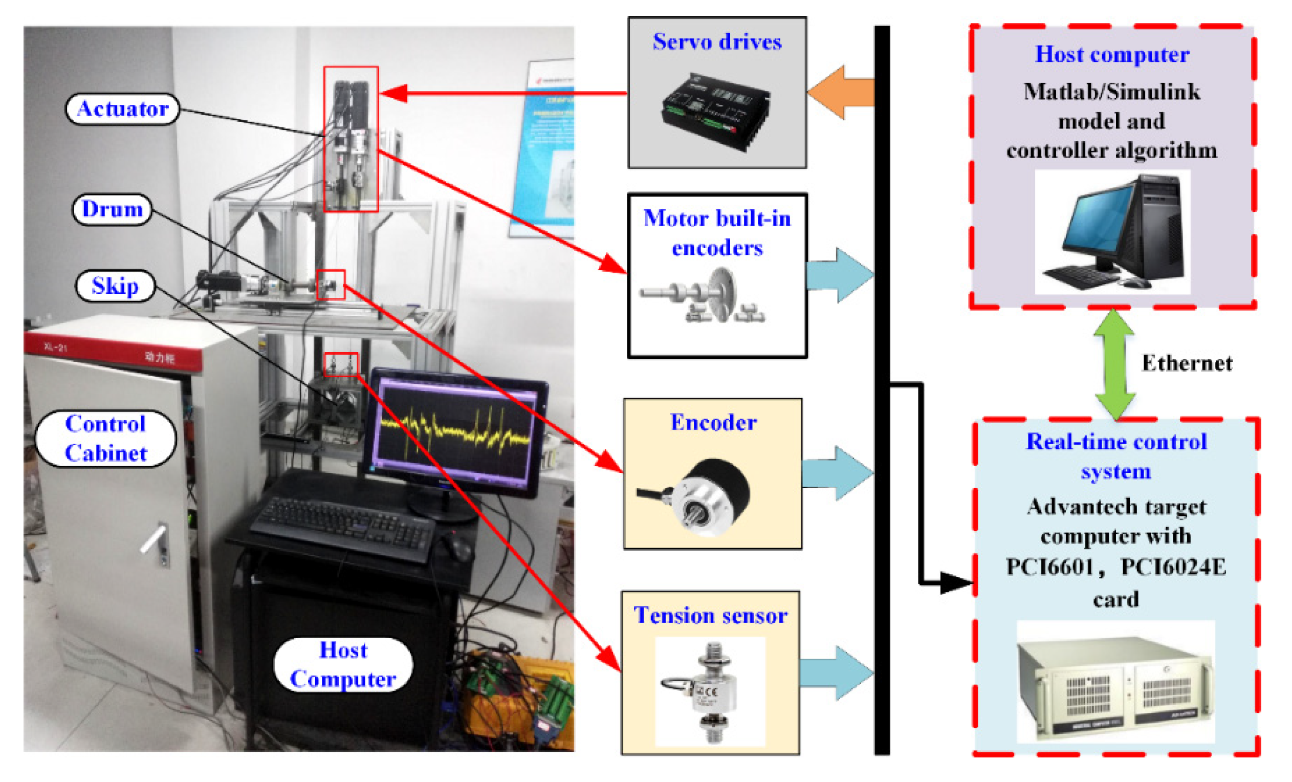
4. Experiment Result and Analysis

To verify the proposed electromechanical actuator fault-tolerant control method, a xpc technology-based experimental system involving the mine hoist mechanical structure, different kinds of sensors, and two computers was built as shown in Figure 6. The tension sensor connects the end of the vertical rope and skip which is used to measure the tension of the wire rope. Three encoders are fixed on the drum shaft end and two headgear sheaves’ shaft end, respectively. Each electric actuator consists of a 400 W motor, a gearbox whose reduction ratio is 1:10, and a screw structure. Sensor signals are acquired by PCI-6601 and PCI-6024E data collection cards which are installed in an Advantech target computer mainboard slot with sampling frequency 1 khz. According to the dimensions and specifications of the experimental system hardware, relevant parameters of the mathematical model can be set as follows: θ_qx = 45°, ${\rho }_{wr}$ = 0.004 kg/m, $r_s^{(i)}$ = 0.03 m, ${\psi }_{mtf}^{(i)}$= 0.32 Wb, $L_{mtd}^{(i)}=L_{mtq}^{(i)}=2.8\hspace{0.17em}\mathrm{mH}$, $J_s^{(i)}$ = 0.005 kg·m², $p_{mt}^{(i)}=4$, $EA=2\times {10}^6$ N.

Considering that the failure of the motor and the electronic unit during the actual operate process takes place inside the equipment, the fault type, time of occurrence, and fault amplitude are not easy to control. Meanwhile, as faults mainly affect the opening response of the electromechanical actuator, add additional disturbance signals to the motor drive input to simulate faults of the right headgear sheave actuator subsystem as follows:

$$\{\begin{array}{c}{f}_{af2}^{\left(2\right)}=-{\mathrm{z}}_{mulf}{i}_{mtq}^{(2)}\\ f_{af1}^{\left(2\right)}=-{\mathrm{z}}_{addf}\sin 5\pi \left(t-2.5\right)\\ f_{af1}^{\left(2\right)}=-{\mathrm{z}}_{addf}\sin 5\pi \left(t-8.2\right)\\ 0\end{array}\begin{array}{c}\\ \\ \\ \end{array}\begin{array}{c}2.5 \mathrm{s}<t<4 \mathrm{s}\\ 2.5 \mathrm{s}<t<4 \mathrm{s}\\ 8.2 \mathrm{s}<t<10.1 \mathrm{s}\\ \mathrm{else}\end{array}\begin{array}{c}\\ \\ \\ \end{array}\begin{array}{c}\mathrm{and}\\ \\ \\ \end{array}\begin{array}{c}\\ \\ \\ \end{array}\begin{array}{c}8.2 \mathrm{s}<t<10.1 \mathrm{s}\\ \\ \\ \end{array}$$

(57)

where ${\mathrm{z}}_{mulf}$ and ${\mathrm{z}}_{addf}$ are fault coefficients and can be modified in the computer program. The reason for picking the birth time of faults is that the difference between the length of the two ropes occurs in the winding process, which can reflect the actuator performance.

To evaluate the performance of the developed actuator fault-tolerant control method for wire rope tension coordination control, two indicators of the root mean square error (RMSE) and maximum absolute error (MAE) are employed for the evaluation. The calculation method of the two indicators can be expressed as

$$\mathrm{RMSE}=\sqrt{{{\displaystyle \sum _{N_{tt}=1}^{N_{ts}}\left|F_{cn,N_{tt}}^{\left(1\right)}-F_{cn,N_{tt}}^{\left(2\right)}\right|}}^2}$$

(58)

$$\mathrm{MAE}=\max {\displaystyle \sum _{N_{tt}=1}^{N_{ts}}\left|F_{cn,N_{tt}}^{\left(1\right)}-F_{cn,N_{tt}}^{\left(2\right)}\right|}$$

(59)

where $F_{cn,N_{tt}}^{\left(i\right)}$ denotes the rope tension value at the N_tt-th sampling point. $N_{ts}$ represents the number of sampling points during the experimental process.

For illustrating the effectiveness of the above fault-tolerant controller design more clearly, the following two controllers are compared.

(1)

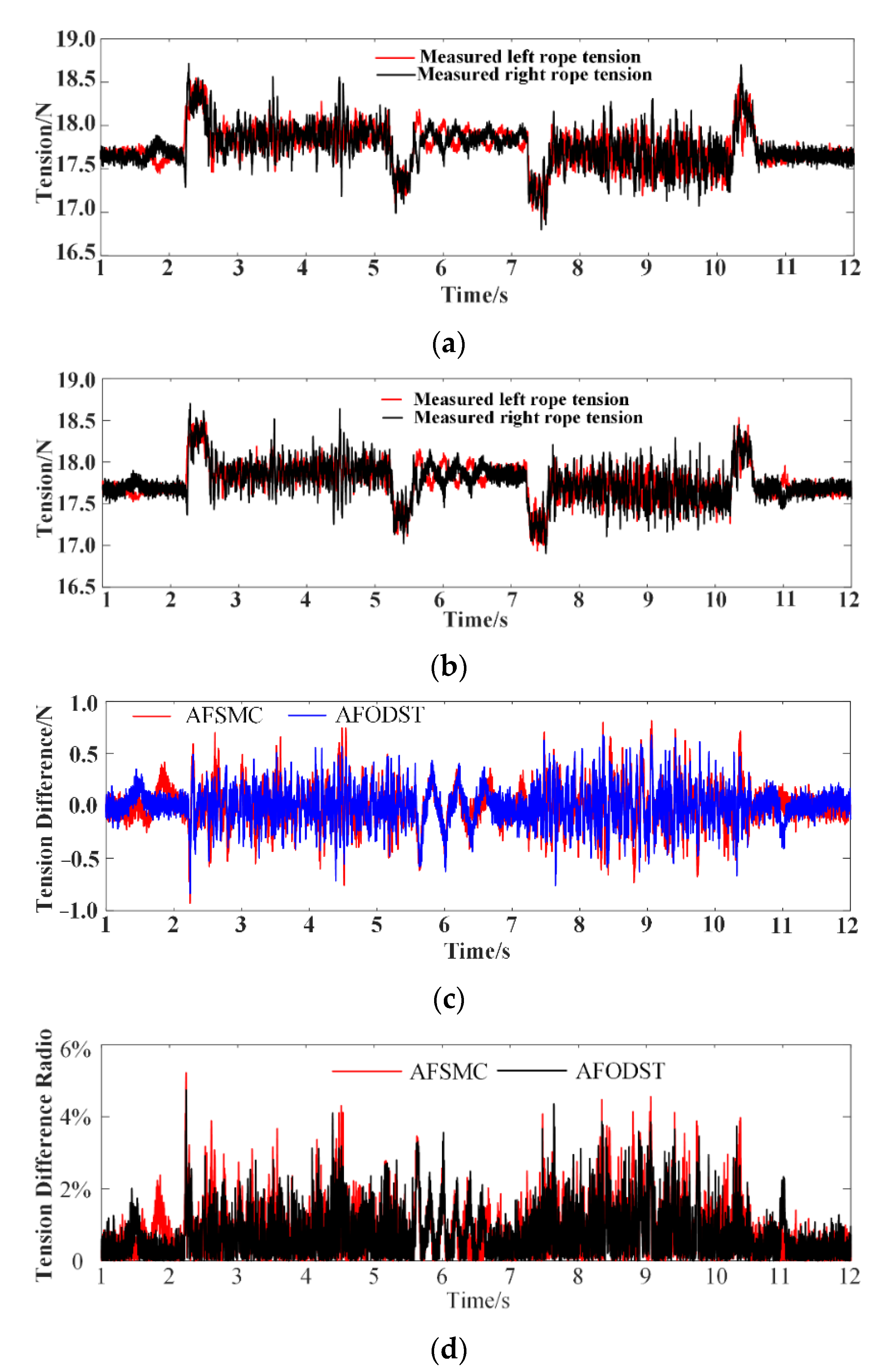
AFSMC: This is the adaptive fuzzy sliding mode controller with a fuzzy smooth switching item as discussed in [48]. The tension coordination control loop applies an improved sliding mode algorithm to overcome the interference, and the actuator control loop employs the traditional proportion-integration-differentiation (PID) algorithm. The input voltage amplitude of the left side actuator is equal to the right side actuator, and the symbols of the two side inputs are opposite. The gains of the controller are chosen as: $K_{af}=2\times {10}^{-5}$, $K_{vf}=2.25$, $K_{df}=0.028$, $\sigma =2.25$, $\gamma =0.042$, $\eta ={10}^{-3}$.

(2)

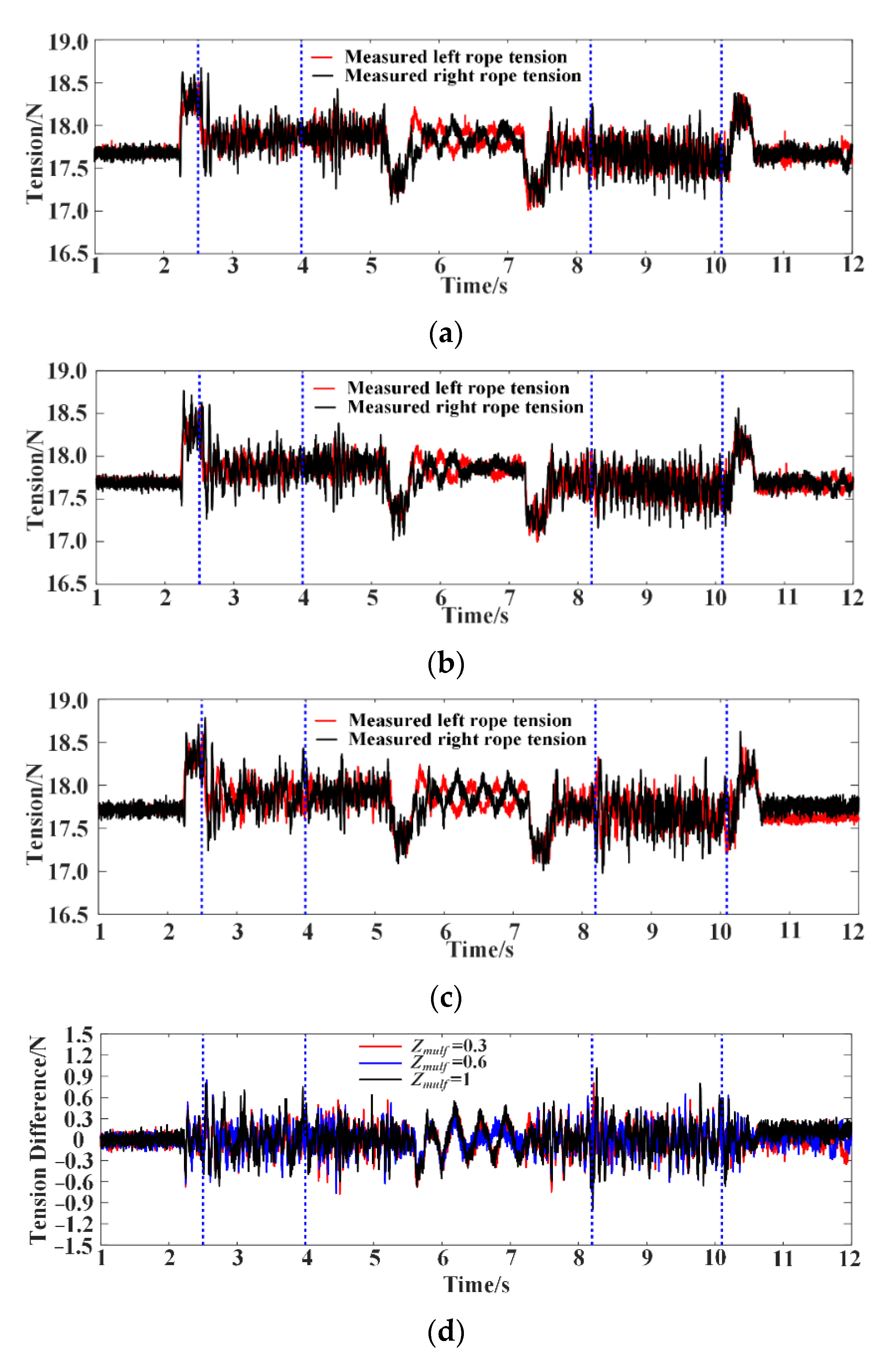
AFODST: This is the adaptive fault observer (12) and dynamic surface technology-based fault tolerant controller (43) proposed in this paper according to the theoretical design procedure. The parameters of the actuator fault observer are obtained by using the LMI toolbox to solve according to formula (15). The final gains are: ${\mathsf{\alpha }}_{fo}^{(1)}={\mathsf{\alpha }}_{fo}^{(2)}=\mathrm{diag}\left({10}^{-2},0.016\right)$, ${\mathsf{\delta }}_{fo}^{(1)}={\mathsf{\delta }}_{fo}^{(1)}=\mathrm{diag}\left(0.003,0.015\right)$, ${\gamma }_{fo}^{(1)}={\gamma }_{fo}^{(2)}=\mathrm{diag}\left(0.06,1.28\right)$, ${\theta }_{fo1}^{\left(1\right)}={\theta }_{fo1}^{\left(2\right)}={10}^{-6}$, ${\theta }_{fo2}^{\left(1\right)}={\theta }_{fo2}^{\left(2\right)}=2\times {10}^{-4}$, $p_{sof1}^{(1)}$ = $p_{sof2}^{(1)}$ = $p_{sof1}^{(2)}$ = $p_{sof2}^{(2)}$ = 3, $p_{xof1}^{(1)}$ = $p_{xof2}^{(1)}$ = $p_{xof1}^{(2)}$ = $p_{xof2}^{(2)}$ = 5. In addition, the gains of the improved dynamic surface fault-tolerant controller are chosen as: ${\vartheta }_{mh2}^{(1)}={\vartheta }_{mh2}^{(1)}={10}^{-3}$, ${\sigma }_{mh2}^{\left(1\right)}={\sigma }_{mh2}^{\left(2\right)}=0.02$, $w_{bd}^{\left(1\right)}=w_{bd}^{\left(2\right)}={10}^3$, ${\sigma }_{mh1}=0.035$, ${\varpi }_{mh1}=2.4$, ${\eta }_{mh1}=2.1\times {10}^{-5}$, ${\varpi }_{mh2}^{\left(1\right)}={\varpi }_{mh2}^{\left(2\right)}=0.035$, ${\chi }_{mh1}^{\left(1\right)}={\chi }_{mh1}^{\left(2\right)}=0.028$, ${\chi }_{mh2}^{\left(1\right)}={\chi }_{mh2}^{\left(2\right)}=0.019$, ${\chi }_{mh3}^{\left(1\right)}={\chi }_{mh3}^{\left(2\right)}=0.026$, ${\eta }_{mh2}^{\left(1\right)}={\eta }_{mh2}^{\left(2\right)}=3\times {10}^{-4}$, ${\rho }_{mh1}=0.035$, ${\rho }_{mh2}^{\left(1\right)}={\rho }_{mh2}^{\left(2\right)}=0.022$.

The rope tension coordination control effect performances under the two controllers in a normal case are shown in Figure 7. As can be seen, the proposed AFODST and AFSMC controllers have approximately the same effect and are better than the traditional PID controller which was used in the literature [49] dealing with random drum winding disturbance since the above two controllers both made use of an adaptive function to adjust the control input and compensate dynamic modeling uncertainties. As shown in Figure 7d, the maximum ratio of the tension difference to the average tension under the effect of the AFSMC is 5.22%, and the maximum ratio under the action of the AFODST is 4.74%; the fluctuation ranges are both within 10%.

The experimental results of two controllers under actuator fault conditions are provided in Figure 8, Figure 9 and Figure 10. In addition, a qualitative comparison of tension control performance indices between the two controllers under four conditions is given in

Table 2. Tension Control Performance indexes.

Controller	RMSE	MAE	RMSE	MAE
	Condition 1—No faults		Condition 2—zaddf = 0.1, zmulf = 0.3
AFSMC	20.062	0.927	22.858	0.997
AFODST	18.171	0.833	18.239	0.803
	Condition 3—zaddf = 0.1, zmulf = 0.6		Condition 4—zaddf = 0.1, zmulf = 1
AFSMC	27.374	1.180	66.527	2.802
AFODST	17.938	0.847	21.399	1.015

. It can be seen that along with the value of the fault parameter z_mulf, increasing from 0.3 to 1, fluctuation ranges for the RMSE and MAE under the action of the AFSMC are [20.062 N~66.527 N] and [0.927 N~2.802 N]. In the case of condition 2, the RMSE and MAE of the tension difference under AFSMC action grew by 13.94 percent and 7.55 percent, respectively, compared with condition 1. The RMSE and MAE rose by 36.45 percent and 27.29 percent with the effect of the AFSMC in the case of condition 3 compared with the no faults condition. With the action of the AFSMC, in the case of condition 4, the RMSE and MAE increased 231.61 percent and 202.27 percent compared with the case of the normal condition. Those indicate that the AFSMC can overcome the set fault $f_{af1}^{\left(2\right)}$ very well; the tension coordination control effect is basically the same as in the no faults condition when amplitudes of the set addition and multiplication electromechanical actuator faults are small (z_addf = 0.1, z_mulf = 0.3). However, the effect is gradually getting worse with the coefficient increase of $f_{af2}^{\left(2\right)}$, as the effectiveness of the single actuator is getting weaker, and the tension compensation effect cannot meet the requirements.

Figure 9 illustrates the outputs of fault observers in the above fault case. In Figure 9a,b, it can be seen that the actuators implement actions in real time to control rope tension, and the states of actuators are well tracked by the estimated state in all cases. Meanwhile, when the actuators are in a normal state, the running state of the actuators is basically maintained in many experiments, and the actuators on both sides carry out the control task together. During the period of actuators’ faults, the right actuator gradually loses control as the fault severity increases; by contrast, the left actuator takes on more of the control task under the action of the fuzzy assignment factor so that the controller can complete the control objectives. Figure 9c,d present the estimation of fault influence factors. It can be noticed that although there is no fault set for the left actuator, there is still a certain fault estimation value, which is caused by modeling error and uncertainties. In addition, when the fault parameter of the right actuator increases, the amplitude of the fault index is also becoming larger, which can be well tracked and estimated. By analyzing the fault observer results in Figure 9, it is obvious that the fault observers have a good fault detection effect for one thing and can effectively guide the control allocation of the controller for another.

From Figure 10, it can be shown that fluctuation ranges for the RMSE and MAE under the action of the proposed strategy are [18.171 N~21.399 N] and [0.803 N~1.015 N]. In the case of condition 2, the RMSE and MAE of the tension difference under AFODST action are reduced by 20.21 percent and 19.46 percent, respectively, compared with under AFSMC action. The RMSE and MAE lessen by 34.47 percent and 28.22 percent with the effect of the AFODST in the case of condition 3 compared with under the action of the AFSMC. With the action of the AFODST, in the case of condition 4, the RMSE and MAE lower 67.83 percent and 63.78 percent compared with under the effect of the AFSMC.

For the experimental results under the four conditions, the superiority of the proposed electromechanical actuator fault-tolerant controller is definitely proven. The proposed strategy can not only effectively overcome the disturbance effect as the conventional controller, it can also reduce the impact of the time-varying actuator fault. From the point of view of the rope tension control effect and controller robustness, the proposed method is more applicable than the comparative AFSMC method to the tension coordination control under variable operating conditions.

5. Conclusions

In this paper, an adaptive dynamic surface technology-based electromechanical actuator fault tolerant scheme is designed for the Blair mine hoist. Comparative experimental results of the proposed strategy with the AFSMC under drum winding disturbance and actuator fault conditions are obtained to illustrate the superiority of the designed hybrid controller under complex conditions in tension coordination controlling. The results of this work can be summarized and concluded as follows:

(1)

According to the actuator fault analysis and dynamic characteristic analysis of the mine hoist tension coordination control system, the overall mathematic model of the system includes the hoisting subsystem, skip subsystem, electric drive actuators, and the electromechanical actuator fault is built and expressed with a state space formulation.

(2)

In order to solve the tension coordination control problem under fault conditions, the RBF neural-network-based adaptive observer is applied to estimate the electromechanical actuator fault state. The hybrid method consists of the adaptive dynamic surface controller, fuzzy allocation factor, and the error barrier function is developed to achieve a better real-time control effect dealing with the sudden fault situation and unexpected disturbance. Each step of this algorithm is explicitly presented, and the stability of the tension coordination closed-loop control system is proved.

(3)

Through the simulated actuator faults’ experimental test, the proposed hybrid strategy shows stronger robustness and reacts faster when an electromechanical actuator performance loss fault occurs. Even when one of the actuators fails completely, the designed controller can achieve almost the same performance as the normal operating conditions. Compared with the AFSMC, the RMSE is reduced by 67.83 percent, and the MAE is reduced by 63.78 percent, in the worst setting situation. The validity of the theoretical analysis is thus verified.

However, since the designed controller contains various parameters that need to be set and adjusted, specific tune rules and optimization algorithms are urgently needed to be developed, which will be the focus in further research. Moreover, the design fault simulation strategy closer to the real situation is also the subsequent exploration direction.

References

1. Giraud, L.; Galy, B. Fault tree analysis and risk mitigation strategies for mine hoists. Saf. Sci. 2018, 110, 222–234. [Google Scholar] [CrossRef]
2. Pi, Y.; Zhang, J.; Tang, X.; Zhu, J. Three-dimensional dynamic modeling and simulation of a multi-cable winding hoister system considering bidirectional coupling between cage and flexible guides. J. Vib. Control 2022. [Google Scholar] [CrossRef]
3. Yao, J.; Ma, Y.; Ma, C.; Xiao, X.; Xu, T. Effect of misalignment failures of steel guides on impact responses in friction mine hoisting systems. Eng. Fail. Anal. 2020, 118, 104841. [Google Scholar] [CrossRef]
4. Peng, X.; Gong, X.S.; Liu, J.J. The study on crossover layouts of multi-layer winding grooves in deep mine hoists based on transverse vibration characteristics of catenary rope. Proc. Inst. Mech. Eng. Part I J. Syst. Control Eng. 2019, 233, 118–132. [Google Scholar] [CrossRef]
5. Chang, X.; Peng, Y.; Zhu, Z.; Gong, X.; Yu, Z.; Mi, Z.; Xu, C. Breaking failure analysis and finite element simulation of wear-out winding hoist wire rope. Eng. Fail. Anal. 2019, 95, 1–17. [Google Scholar] [CrossRef]
6. Wang, J.; Pi, Y.; Krstic, M. Balancing and suppression of oscillations of tension and cage in dual-cable mining elevators. Automatica 2018, 98, 223–238. [Google Scholar] [CrossRef]
7. Zhu, Z.C.; Li, X.; Shen, G.; Zhu, W.D. Wire rope tension control of hoisting systems using a robust nonlinear adaptive backstepping control scheme. ISA Trans. 2018, 72, 256–272. [Google Scholar] [CrossRef]
8. Chen, X.; Zhu, Z.C.; Li, W.; Shen, G. Fault-tolerant control of double-rope winding hoists combining neural-based adaptive technique and iterative learning method. IEEE Access 2019, 7, 50476–50491. [Google Scholar] [CrossRef]
9. Li, X.; Zhu, Z.; Shen, G.; Tang, Y. Wire Tension Coordination Control of Electro-Hydraulic Servo Driven Double-Rope Winding Hoisting Systems Using a Hybrid Controller Combining the Flatness-Based Control and a Disturbance Observer. Symmetry 2021, 13, 716. [Google Scholar] [CrossRef]
10. Ding, X.; Shen, G.; Tang, Y.; Li, X. Axial vibration suppression of wire-ropes and container in double-rope mining hoists with adaptive robust boundary control. Mechatronics 2022, 85, 102817. [Google Scholar] [CrossRef]
11. Zang, W.; Shen, G.; Rui, G.; Li, X.; Li, G.; Tang, Y. A flatness-based nonlinear control scheme for wire tension control of hoisting systems. IEEE Access 2019, 7, 146428–146442. [Google Scholar] [CrossRef]
12. Wang, J.; Pi, Y.; Hu, Y.; Zhu, Z. State-observer design of a PDE-modeled mining cable elevator with time-varying sensor delays. IEEE Trans. Control Syst. Technol. 2019, 28, 1149–1157. [Google Scholar] [CrossRef]
13. Ding, S.X.; Li, L. Control performance monitoring and degradation recovery in automatic control systems: A review, some new results, and future perspectives. Control Eng. Pract. 2021, 111, 104790. [Google Scholar] [CrossRef]
14. Shen, Q.; Yue, C.; Goh, C.H.; Wang, D. Active fault-tolerant control system design for spacecraft attitude maneuvers with actuator saturation and faults. IEEE Trans. Ind. Electron. 2018, 66, 3763–3772. [Google Scholar] [CrossRef]
15. Wang, Y.; Jiang, B.; Wu, Z.G.; Xie, S.; Peng, Y. Adaptive sliding mode fault-tolerant fuzzy tracking control with application to unmanned marine vehicles. IEEE Trans. Syst. Man Cybern. Syst. 2020, 51, 6691–6700. [Google Scholar] [CrossRef]
16. Tian, G.; Yuan, G.; Aleksandrov, A.; Zhang, T.; Li, Z.; Fathollahi-Fard, A.M.; Ivanov, M. Recycling of spent Lithium-ion Batteries: A comprehensive review for identification of main challenges and future research trends. Sustain. Energy Technol. Assess. 2022, 53, 102447. [Google Scholar] [CrossRef]
17. Chen, Z.; Yang, X.; Liu, X. RBFNN-based nonsingular fast terminal sliding mode control for robotic manipulators including actuator dynamics. Neurocomputing 2019, 362, 72–82. [Google Scholar] [CrossRef]
18. Amin, A.A.; Hasan, K.M. A review of fault tolerant control systems: Advancements and applications. Measurement 2019, 143, 58–68. [Google Scholar] [CrossRef]
19. Gao, Z.; Cecati, C.; Ding, S.X. A survey of fault diagnosis and fault-tolerant techniques—Part I: Fault diagnosis with model-based and signal-based approaches. IEEE Trans. Ind. Electron. 2015, 62, 3757–3767. [Google Scholar] [CrossRef] [Green Version]
20. Chen, T.; Chen, L.; Xu, X.; Cai, Y.; Jiang, H.; Sun, X. Passive fault-tolerant path following control of autonomous distributed drive electric vehicle considering steering system fault. Mech. Syst. Signal Process. 2019, 123, 298–315. [Google Scholar] [CrossRef]
21. Başak, H.; Kemer, E.; Prempain, E. A passive fault-tolerant switched control approach for linear multivariable systems: Application to a quadcopter unmanned aerial vehicle model. J. Dyn. Syst. Meas. Control 2020, 142, 031004. [Google Scholar] [CrossRef]
22. Hu, C.; Wei, X.; Ren, Y. Passive fault-tolerant control based on weighted LPV tube-MPC for air-breathing hypersonic vehicles. Int. J. Control Autom. Syst. 2019, 17, 1957–1970. [Google Scholar] [CrossRef]
23. Hao, L.Y.; Zhang, H.; Li, T.S.; Lin, B.; Chen, C.L.P. Fault tolerant control for dynamic positioning of unmanned marine vehicles based on TS fuzzy model with unknown membership functions. IEEE Trans. Veh. Technol. 2021, 70, 146–157. [Google Scholar] [CrossRef]
24. Aydin, M.N.; Coban, R. PID sliding surface-based adaptive dynamic second-order fault-tolerant sliding mode control design and experimental application to an electromechanical system. Int. J. Control 2022, 95, 1767–1776. [Google Scholar] [CrossRef]
25. Abbaspour, A.; Mokhtari, S.; Sargolzaei, A.; Yen, K.K. A survey on active fault-tolerant control systems. Electronics 2020, 9, 1513. [Google Scholar] [CrossRef]
26. Xiao, B.; Yin, S. A deep learning based data-driven thruster fault diagnosis approach for satellite attitude control system. IEEE Trans. Ind. Electron. 2020, 68, 10162–10170. [Google Scholar] [CrossRef]
27. Rudin, K.; Ducard GJ, J.; Siegwart, R.Y. Active fault-tolerant control with imperfect fault detection information: Applications to UAVs. IEEE Trans. Aerosp. Electron. Syst. 2019, 56, 2792–2805. [Google Scholar] [CrossRef]
28. Abbaspour, A.; Yen, K.K.; Forouzannezhad, P.; Sargolzaei, A. A neural adaptive approach for active fault-tolerant control design in UAV. IEEE Trans. Syst. Man Cybern. Syst. 2018, 50, 3401–3411. [Google Scholar] [CrossRef]
29. Xiong, H.; Liao, Y.; Chu, X.; Nian, X.; Wang, H. Observer based fault tolerant control for a class of Two-PMSMs systems. ISA Trans. 2018, 80, 99–110. [Google Scholar] [CrossRef] [PubMed]
30. Nguyen, V.-C.; Tran, X.-T.; Kang, H.-J. A Novel High-Speed Third-Order Sliding Mode Observer for Fault-Tolerant Control Problem of Robot Manipulators. Actuators 2022, 11, 259. [Google Scholar] [CrossRef]
31. Han, J.; Liu, X.; Wei, X.; Sun, S. A dynamic proportional-integral observer-based nonlinear fault-tolerant controller design for nonlinear system with partially unknown dynamic. IEEE Trans. Syst. Man Cybern. Syst. 2021, 52, 5092–5104. [Google Scholar] [CrossRef]
32. Lei, Q.; Ma, Y.; Liu, J.; Yu, J. Neuroadaptive observer-based discrete-time command filtered fault-tolerant control for induction motors with load disturbances. Neurocomputing 2021, 423, 435–443. [Google Scholar] [CrossRef]
33. Truong, H.V.A.; Ahn, K.K. Actuator failure compensation-based command filtered control of electro-hydraulic system with position constraint. ISA Trans. 2022. [Google Scholar] [CrossRef]
34. Li, L.; Yao, L.; Wang, H.; Gao, Z. Iterative learning fault diagnosis and fault tolerant control for stochastic repetitive systems with Brownian motion. ISA Trans. 2022, 121, 171–179. [Google Scholar] [CrossRef]
35. Chen, X.; Zhu, Z.-C.; Ma, T.-B.; Shen, G. Model-based sensor fault detection, isolation and tolerant control for a mine hoist. Meas. Control 2022, 55, 274–287. [Google Scholar] [CrossRef]
36. Guzmán-Rabasa, J.A.; López-Estrada, F.R.; González-Contreras, B.M.; Valencia-Palomo, G.; Chadli, M.; Pérez-Patricio, M. Actuator fault detection and isolation on a quadrotor unmanned aerial vehicle modeled as a linear parameter-varying system. Meas. Control 2019, 52, 1228–1239. [Google Scholar] [CrossRef] [Green Version]
37. Mao, Z.; Yan, X.G.; Jiang, B.; Chen, M. Adaptive fault-tolerant sliding-mode control for high-speed trains with actuator faults and uncertainties. IEEE Trans. Intell. Transp. Syst. 2019, 21, 2449–2460. [Google Scholar] [CrossRef] [Green Version]
38. Shiravani, F.; Alkorta, P.; Cortajarena, J.A.; Barambones, O. An Enhanced Sliding Mode Speed Control for Induction Motor Drives. Actuators 2022, 11, 18. [Google Scholar] [CrossRef]
39. Wang, Y.; Xu, N.; Liu, Y.; Zhao, X. Adaptive fault-tolerant control for switched nonlinear systems based on command filter technique. Appl. Math. Comput. 2021, 392, 125725. [Google Scholar] [CrossRef]
40. Zhao, Z.; Ren, Y.; Mu, C.; Zou, T.; Hong, K.-S. Adaptive neural-network-based fault-tolerant control for a flexible string with composite disturbance observer and input constraints. IEEE Trans. Cybern. 2021. [Google Scholar] [CrossRef]
41. Huang, J.; Cao, Y.; Xiong, C.; Zhang, H.-T. An echo state Gaussian process-based nonlinear model predictive control for pneumatic muscle actuators. IEEE Trans. Autom. Sci. Eng. 2018, 16, 1071–1084. [Google Scholar] [CrossRef]
42. Guo, Y.; Zhang, D.; Zhang, X.; Wang, S.; Ma, W. Experimental study on the nonlinear dynamic characteristics of wire rope under periodic excitation in a friction hoist. Shock Vib. 2020, 2020, 8506016. [Google Scholar] [CrossRef] [Green Version]
43. Chaoui, H.; Khayamy, M.; Okoye, O. Adaptive RBF network based direct voltage control for interior PMSM based vehicles. IEEE Trans. Veh. Technol. 2018, 67, 5740–5749. [Google Scholar] [CrossRef]
44. Qiao, G.; Liu, G.; Shi, Z.; Wang, Y.; Ma, S.; Lim, T.C. A review of electromechanical actuators for More/All Electric aircraft systems. Proc. Inst. Mech. Eng. Part C: J. Mech. Eng. Sci. 2018, 232, 4128–4151. [Google Scholar] [CrossRef] [Green Version]
45. Smaeilzadeh, S.M.; Golestani, M. A finite-time adaptive robust control for a spacecraft attitude control considering actuator fault and saturation with reduced steady-state error. Trans. Inst. Meas. Control 2019, 41, 1002–1009. [Google Scholar] [CrossRef]
46. Costa, T.V.; Sencio, R.R.; Oliveira-Lopes, L.C.; Silva, F.V. Fault-tolerant control by means of moving horizon virtual actuators: Concepts and experimental investigation. Control Eng. Pract. 2021, 107, 104683. [Google Scholar] [CrossRef]
47. Edalati, L.; Sedigh, A.K.; Shooredeli, M.A.; Moarefianpour, A. Adaptive fuzzy dynamic surface control of nonlinear systems with input saturation and time-varying output constraints. Mech. Syst. Signal Process. 2018, 100, 311–329. [Google Scholar] [CrossRef]
48. Li, X.; Zhu, Z.C.; Shen, G. A switching-type controller for wire rope tension coordination of electro-hydraulic-controlled double-rope winding hoisting systems. Proc. Inst. Mech. Eng. Part I J. Syst. Control Eng. 2016, 230, 1126–1144. [Google Scholar] [CrossRef]
49. Chen, X.; Zhu, Z.; Shen, G.; Li, W. Tension coordination control of double-rope winding hoisting system using hybrid learning control scheme. Proc. Inst. Mech. Eng. Part I J. Syst. Control Eng. 2019, 233, 1265–1281. [Google Scholar] [CrossRef]
50. Huang, J.; Luo, C.; Yu, P.; Hao, H. A methodology for calculating limit deceleration of flexible hoisting system: A case study of mine hoist. Proc. Inst. Mech. Eng. Part E Ournal Process Mech. Eng. 2020, 234, 342–352. [Google Scholar] [CrossRef]
Figure 1. The structure of Blair mine hoist.
Actuators 11 00299 g001
Figure 2. Mine hoist dynamic model. (a) Hoisting subsystem model; (b) Skip subsystem model; (c) Electric drive actuator model.
Actuators 11 00299 g002
Figure 3. Fault Tree of Electromechanical Actuators in Tension Coordination Control System.
Actuators 11 00299 g003
Figure 4. Overall Architecture of Electromechanical Actuators Fault-Tolerant Control System.
Actuators 11 00299 g004
Figure 5. Radial Basis Neural Network Structure.
Actuators 11 00299 g005
Figure 6. xpc-based mine hoist platform.
Actuators 11 00299 g006
Figure 7. Measured rope tension and tension difference under normal condition: (a) Rope tension with AFSMC; (b) Rope tension with AFODST; (c) Tension difference; (d) Ratio of the tension difference to the average tension.
Actuators 11 00299 g007
Figure 8. Measured rope tension and tension difference under fault condition with AFSMC: (a) Zmulf = 0.3; (b) Zmulf = 0.6; (c) Zmulf = 1; (d) Tension difference.
Actuators 11 00299 g008
Figure 9. Fault observer output under fault conditions: (a) Estimated state of left actuator; (b) Estimated state of right actuator; (c) Fault estimation output of left actuator; (d) Fault estimation output of right actuator.
Actuators 11 00299 g009
Figure 10. Measured rope tension and tension difference under fault condition with AFODST: (a) Zmulf = 0.3; (b) Zmulf = 0.6; (c) Zmulf = 1; (d) Tension difference.
Actuators 11 00299 g010