Design and Experiment Evaluation of Load Distribution on the Dual Motors in Cam-Based Variable Stiffness Actuator with Helping Mode

Abstract

This paper presents a novel cam-based variable stiffness actuator (VSA). It significantly differs from its counterparts in that the external load distributes on its two motors with a small difference. It is a feasible method to improve VSA’s output power, especially in compact joints, such as rehabilitation devices. The stiffness adjustment involves a spring-balanced crank-slider mechanism with a variable-length base frame. Its tunable node is the common node for force decomposition, synthesis, stiffness adjustment, and position control by setting it at the common groove of two differential variable-pitch cams. The paper establishes analytical expressions among the pressure angle of the cam pitch curve, load distribution, and its crucial design indexes and constraints. Based on this, the pitch curve synthesis method is put forward to optimize the load distribution. In addition, a reasonable tradeoff can be easily made by locally adjusting the cam pressure angle. So, the dual motors can work against the output load together in the same direction with a close amount. In the fabricated prototype, current stratification caused by the unstable friction direction has been observed. The estimation results of motor frictionless current matched the designed load distribution behavior.

1. Introduction

Compared with traditional rigid actuators, compliant actuators exhibit superior interactive performance such as elastic muscles [1,2,3]. They are widely researched in wearable applications, such as assistive exoskeleton [4,5] and rehabilitation devices [6,7]. As the simplest compliant actuator in its early stage, the series elastic actuator (SEA) has linear springs intentionally placed between the motor and actuator output. It turns the force control problem into a position control one [8]. This results in simple force control, great shock-absorbing, inherent security, low-energy consumption in cyclic movements, and velocity gain in explosive movements [9,10,11]. By introducing the stiffness adjustment module, the variable stiffness actuator (VSA) broadens the stiffness range and furtherly improves the torque control bandwidth [12,13] and dynamic performance [14,15].

However, the size, weight, and costs conflict with five other attributes that describe a VSA, i.e., output power, potential energy storage, stiffness range, efficiency, and accuracy [16]. After tradeoff design, numerous VSAs were developed to address various demands on their functionality. In addition, these designs were classified in detail according to their principles [17] and became important guidelines to their successors. VSA generally includes two motors to achieve synchronous control of stiffness and torque (or position). The size, output power, and efficiency are directly related to the load distribution on the two motors—the more evenly the load distribution, the better. For in-depth research of the load distribution, this paper re-divides the VSA into the following three categories: the VSA with independent mode (Figure 1a), the VSA with antagonistic mode (Figure 1b), and the VSA with helping mode (Figure 1c).

For the VSA with independent mode, its output load is entirely supported by a high-power prime motor. A small-power auxiliary motor drives the stiffness adjustment mechanism. Its adjustment principles include the followings: tuning spring preload (VSM [18], RVSA [19]), varying the attachment points of the internal springs (AWAS [20]), moving the pivot point (SVSA-II [21], VSA with variable-link [22], CRM-VSA [23]), changing the physical properties of the spring [24,25,26]. These actuators received broad focus for their force decoupling structure: force F_M2 perpendicular to F_M1 at two independent nodes for two control variables (Figure 1a). It substantially simplifies the control strategy. However, the decoupling feature also makes the auxiliary motor no longer support the prime motor.

For the VSA with antagonistic mode, its output load equals the difference value of dual prime motors’ output [27,28]. The two motors drive the output shaft through non-linear springs with two antagonistic nodes [29,30]. Both the nodes can act on stiffness and position adjustment, but with opposite forces (F_M1 and F_M2 in Figure 1b). Rotation of the motors, in the same sense, generates a net output torque, while counter-rotation sets different stiffness [31]. This arrangement allows both motors to contribute to the stiffness adjustment and obtains a flexible structure by cable driving [32,33,34]. However, it also has a drawback: the motors work in antagonistic mode. Its enhanced versions include cross-coupled arrangement and bidirectional layout [35]. Significantly, the latter results in an additional mode called the helping mode. In this case, the maximum torque at the output shaft equals the sum of the two motors in a partial workspace.

For the VSA with helping mode, its output load equals the sum of dual prime motors output in the whole workspace. It arises from some unique structure designs: a force resolving generator at the output of each motor, a common node for force resolving, synthesis, position control, and stiffness adjustment. In Figure 1c, this paper deliberately decomposes the common node into three nodes for a more explicit description according to its function. On node I, the force generator resolves the output force of each motor (F_M1 and F_M2 in Figure 1c) into two orthogonal directions: one for position control ($F_{M1}^d$ and $F_{M2}^d$ in Figure 1c) and another for stiffness adjustment ($F_{M1}^a$ and $F_{M2}^a$ in Figure 1c). Then the position force components couple at node II for a bigger output ($F_{M1}^d+F_{M2}^d$). In addition, on the node III, the net value of the stiffness force components contributes to the stiffness adjustment ($F_{M1}^a-F_{M2}^a$ or $F_{M2}^a-F_{M1}^a$ for two opposite deflection direction).

Moreover, it is also crucial to reduce the load distribution difference between the two motors, i.e., F_M1 and F_M2 should be as close as possible. This is very helpful in fully exploiting the two motors for output power enhancement. Another benefit can be easily guessed but not strictly: the smaller the load distribution difference, the higher the efficiency, for that heat loss is proportional to the square of the motor current. To our knowledge, the research on the VSA with helping mode in the whole workspace is very few. A classical case is the VSJ in literature [36]. However its focus is not on the load distribution. Therefore, this work aims to introduce a novel cam-based VSA with the following advantages:

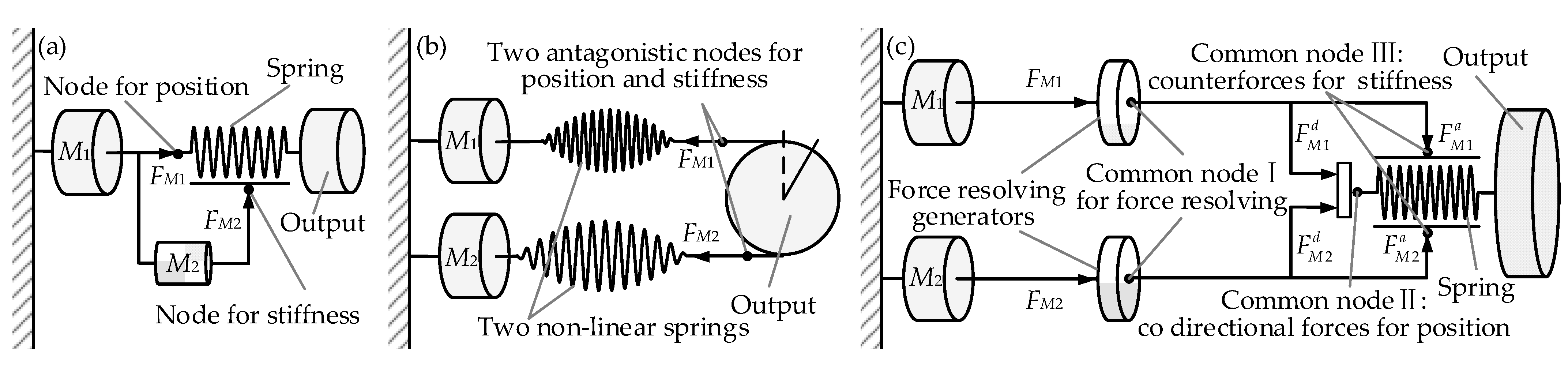
• Antagonistic action for stiffness adjustment, cooperative support for the external load. The VSA shares a common node, as shown in Figure 1c. The force resolving generators are two symmetrical differential cams. On this node, the counter-force of the stiffness adjustment is balanced by the difference of the dual cams’ force components in the joints’ radial direction; the external load is supported by the sum of the cams’ force components in the joints’ tangential direction.
• Load distribution with a small difference for a higher-level helping mode. The ratio between stiffness adjustment counter-force and output counter-force in the crank-slider mechanism can be analytically expressed. Regarding this ratio, the pressure angle of the cam pitch curve is minimized to reduce the load distribution difference on the dual motors.
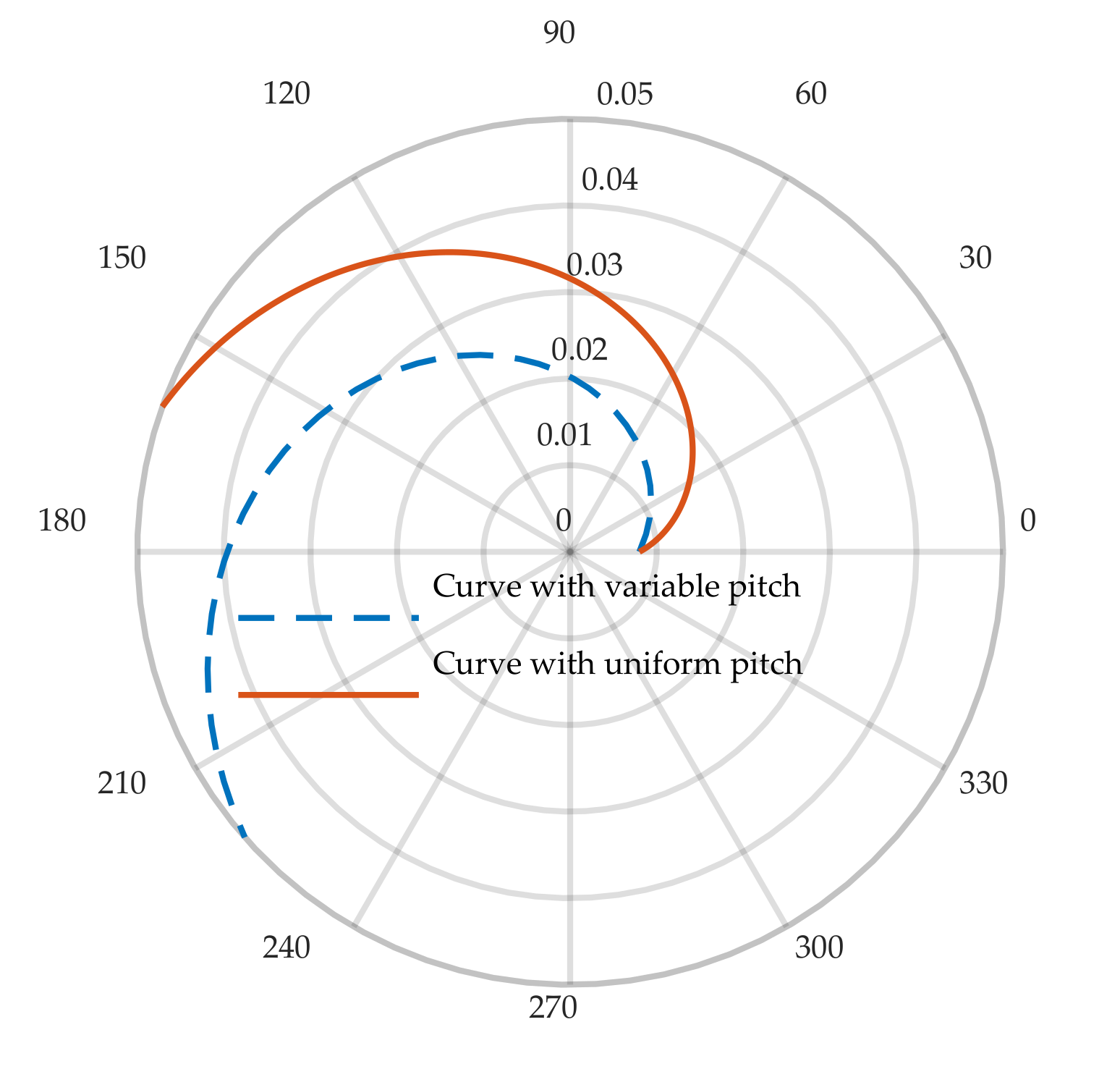
• Reasonable tradeoff design. Different from the strong constraint curve (such as Archimedes spiral), the pressure angle of the pitch curve can be adjusted arbitrarily to meet different design requirements and constraints, such as stiffness adjustment speed, cam local load, curvature radius of the pitch curve and load distribution. A well tradeoff can be made.

The reminder is organized as follows. Section 2 presents the principle and mechanical design. Section 3 describes the load distribution modeling. Section 4 exhibits cam curve synthesis for a more uniform load distribution. The experimental is carried out to evaluate the design result in Section 5. Finally, the conclusion is provided in Section 6.

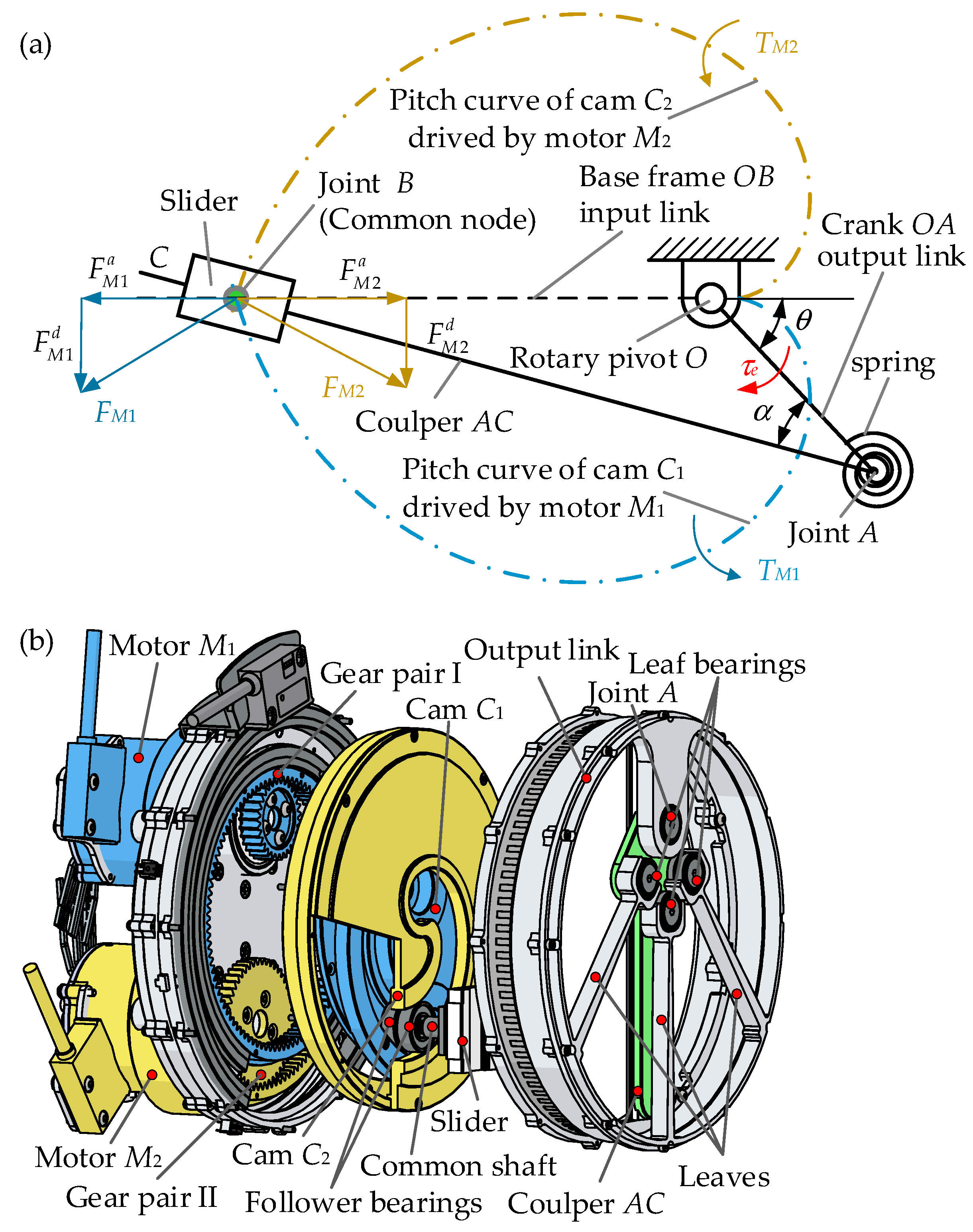
2. Principle and Mechanical Design of the Cam-Based VSA with Helping Mode

The principle of the proposed VSA is illustrated in Figure 2a and meets the structure design characteristic of the VSA with the helping mode in Figure 1c. It can be described in two main levels. In the first level, the variable stiffness module is realized. It includes a typical crank-slider mechanism and a spring between the crank OA and coupler AC. The crank OA acts as the output link, and the base frame OB acts as the input link. The difference between the output link and input link is the deflection angle of the VSA, and the angle between crank OA and coupler AC is the deflection angle of the spring (θ and α in Figure 2a). τ_e is the external load of the VSA and its output stiffness is defined by K = dτ_e/dθ. By changing the length of frame OB, the transmission ratio (dα/dθ) can be regulated, and so the stiffness [37]. Joint B is the common node for stiffness and position control and the point connected to the second level. The second level comprises two symmetrical variable-pitch cams driven by two motors (cams C₁, C₂ and motors M₁, M₂ in Figure 2a). On joint B, the external load τ_e is balanced by the two cams with torques T_M1 and T_M2 in the same direction, i.e., τ_e = T_M1 + T_M2. The cams act as the force generator shown in Figure 1c, and resolve the output force of each motor into two orthogonal directions: one for position control ($F_{M1}^d$ and $F_{M2}^d$ in Figure 2a) and another for stiffness adjustment ($F_{M1}^a$ and $F_{M2}^a$ in Figure 2a). At the same time, the length of OB can be adjusted by a differential rotation of the dual cams.

The exploded view of the CAD model is shown in Figure 2b. The differential cams consist of two independent kinematic chains (colored by blue and yellow, respectively). Motor M₁ devotes to setting the cam C₁ position, and motor M₂ to set the cam C₂ position. M₁ is a frameless DC motor with a torque constant of 36.9 mN/A and connected to a harmonic gear (CSD-17-50-2A-R, with a ratio of 50:1). The output of the harmonic gear is then connected to the cam C₁ through gear pair I with a ratio of 100:29. The two chains have the same structure. The only differences are that the ratio of gear pair II is 130:47, and the torque constant of M₂ is 25.1 mN/A. There is a magnetic ring encoder at the input shaft of the two motors, respectively, with 3200 pulses per turn. It can provide a detection accuracy of 0.001° for cam C₁ and C₂ neglecting the backlash after gear reduction. Joint B is a combination of two cam follower bearings, with a diameter of 19 mm and a rated load of 950 N. The outer rings of two follower bearings are set at the common groove of the cams and its inner rings are mounted on the slider through a common shaft. The slider can move along coupler AC, and the latter forms joint A with the output link. For high compactness, the torsional spring is not an independent part, but a synergy result of two adjacent parts developed from the stiffness adjustment module (leaves on the output link and leaf bearings on the coupler AC in Figure 2b) [38]. The specifications of the variable stiffness module are shown in

Table 1. Specifications of the variable stiffness module.

Description	Symbol	Value
Spring stiffness	ks	85 Nm/rad
Angular deflection range of the spring	α	0~0.22 rad
Range of the output load	τo	0~20 Nm
Length of the crank OA	a	0.04 m
Length range of the base frame OB	ρ	0.008~0.05 m
Rated load of cam followers	[Fb]	950 N
Diameter of cam followers	D	0.019 m

.

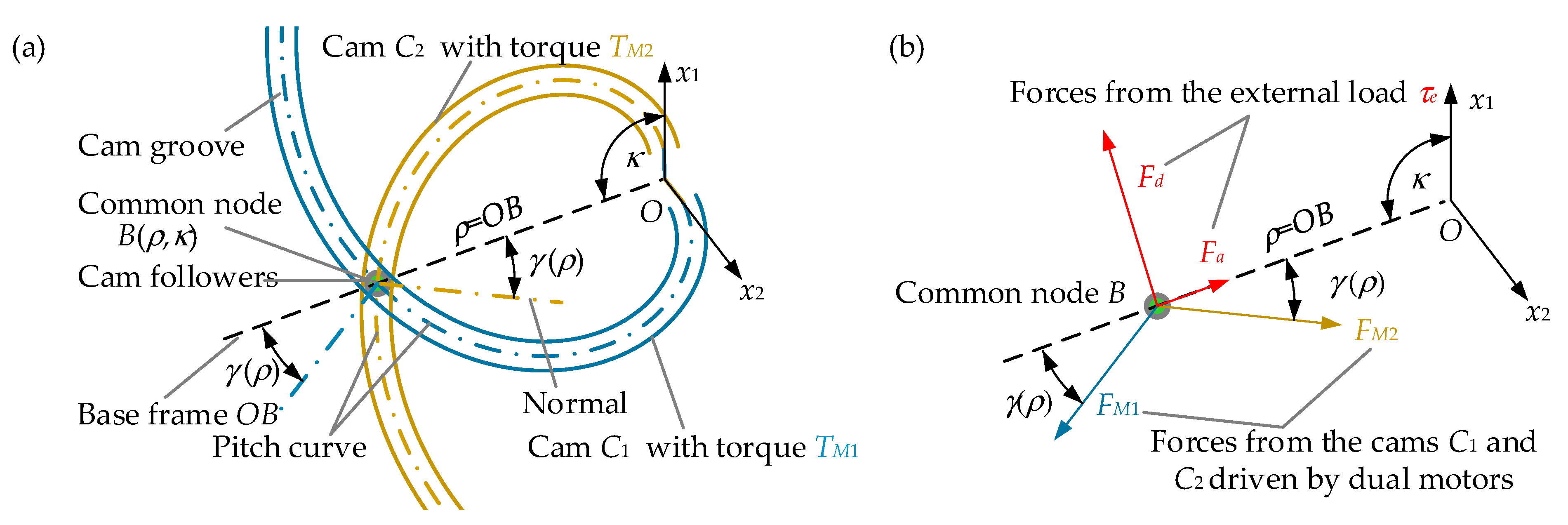
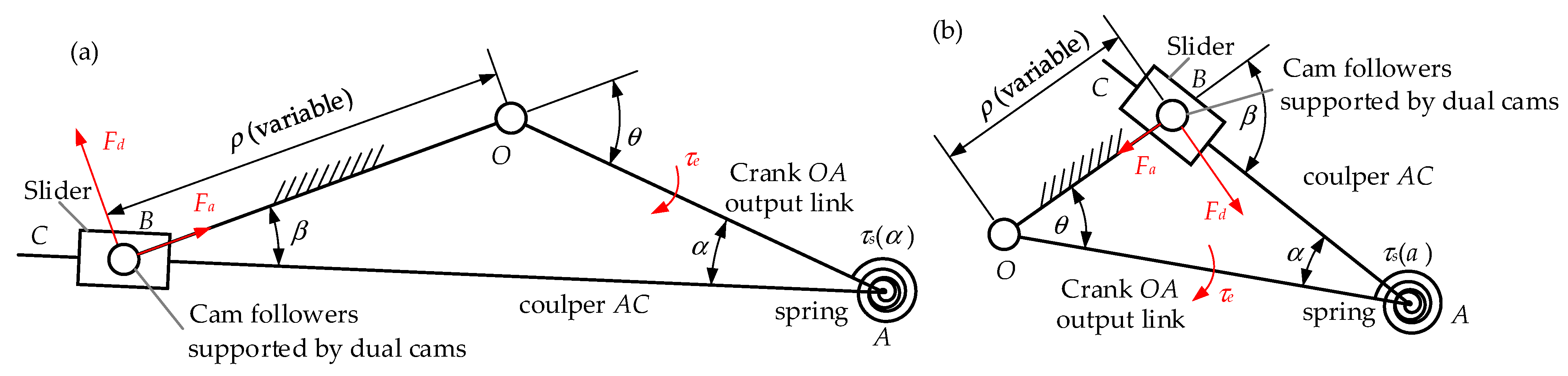
3. The Load Distribution Modeling in a Polar Coordinate System

In this paper, the pitch curves of cam C₁ and C₂ are modeled in the part polar coordinate systems (Figure 3a). Their poles are at the same point O, and polar axes are denoted by x₁ and x₂, respectively. The common node B is located at the cross point of the two pitch curves and is represented by polar coordinate (ρ,κ). ρ is defined as the radial distance for stiffness adjustment (ρ = OB) and κ is the polar angle corresponding to ρ. On the common node, the angular difference between the cam’s normal and the frame OB is the pressure angle of the pitch curve (γ(ρ) in Figure 3a).

There is a general relationship among ρ, κ, γ (ρ) as,

$$\kappa ={\displaystyle \underset{{\rho }_{\min }}{\overset{\rho }{\int }}\frac{1}{\rho tan\left(\gamma (\rho )\right)}d\rho }$$

(1)

Corresponding to the case in Figure 2a, the static forces at the common node is illustrated in Figure 3b. The force from the external load (τ_e) on the followers is decomposed radially and tangentially as F_d, F_a, which is called the position balance counter-force and stiffness adjustment counter-force, respectively. F_M1, F_M2 are the balanced force exerted on the followers by cams C₁ and C₂ in its normal direction. Their relationship is written as,

$$\{\begin{array}{l}{F}_{M1}\sin \gamma (\rho )+F_{M2}\sin \gamma (\rho )=F_d\\ F_{M1}\cos \gamma (\rho )-F_{M2}\cos \gamma (\rho )=F_a\end{array}$$

(2)

f(ρ,θ) is defined to characterize the mechanical property of stiffness adjustment, i.e., f (ρ,θ) = F_a/F_d. Then, there leaves,

$$\{\begin{array}{l}{F}_{M1}=F_d\left(1+f(\rho ,\theta )\tan \gamma (\rho )\right)/2\sin \gamma (\rho )\\ F_{M2}=F_d\left(1-f(\rho ,\theta )\tan \gamma (\rho )\right)/2\sin \gamma (\rho )\end{array}$$

The torques T_M1, T_M2 corresponding to forces F_M1, F_M2 on the cams C₁ and C₂ are,

$$\{\begin{array}{l}{T}_{M1}=F_{M1}\sin \gamma (\rho )\rho ={\tau }_e\left(1+f(\rho ,\theta )\tan \gamma (\rho )\right)/2\\ T_{M2}=F_{M2}\sin \gamma (\rho )\rho ={\tau }_e\left(1-f(\rho ,\theta )\tan \gamma (\rho )\right)/2\end{array}$$

(3)

where τ_e is expressed as τ_e = F_d ρ.

The load ratio ϕ is defined as the smaller value of the torques on the cams over its bigger one, which can characterize the load distribution on the dual motors. When θ < 0, there is T_M1 > T_M2. Then ϕ can be,

$$\varphi =\frac{T_{M2}}{T_{M1}}=\frac{1-f(\rho ,\theta )\tan \gamma (\rho )}{1+f(\rho ,\theta )\tan \gamma (\rho )}$$

(4)

When θ > 0, there is T_M 1 < T_M 2. The corresponding load ratio is,

$$\varphi =\frac{T_{M1}}{T_{M2}}=\frac{1-f(\rho ,\theta )\tan \gamma (\rho )}{1+f(\rho ,\theta )\tan \gamma (\rho )}$$

(5)

From the aspect of load distribution, Equations (4) and (5) have the same physical meaning. So, it only needs to discuss the case in Figure 2a, i.e., θ < 0. According to Equation (4), the operation mode of the VSA is decided by the ϕ, as

Table 2. The relationship between the operation mode of the VSA and its load ratio.

Range of ϕ	ϕ = 1	0 < ϕ < 1	ϕ = 0	ϕ < 0
Operation mode	Ideal helping mode	Normal helping mode	Independent mode	Antagonistic mode
Load distribution	TM1 = τe/2, TM2 = τe/2	0 < TM2 < τe/2, τe/2 < TM1 < te	TM2 = 0, TM 1 = τe	TM2 < 0, TM1 > τe

shows.

Four cases of the load distribution can be imagined. First, ϕ = 1. The dual motors contribute equal to the external load. This is an ideal state. However, the stiffness can never be adjusted as γ (ρ) is always zero. Second, 0 < ϕ < 1. The dual motors share the external load in the same direction with a different amount. Third, ϕ = 0. Only one motor compensates for the external load, while the second motor is idle. Fourth, ϕ < 0. The motors work against each other, and the difference between the two torques generates a net torque at the output link.

A feasible choice assumes the second case. The load ratio ϕ should be very close to 1, for a higher-level help mode. It requires the pressure angle γ (ρ) to be minimized. Another crucial factor is f (ρ,θ). We expect the f (ρ,θ) to be as small as possible. This is also required by the most VSAs. From this aspect, the variable stiffness module based on the crank-slider mechanism is not the best choice. However, it has some other important advantages: an analytical expression of the f (ρ,θ) and easy online reconfiguration. This is very conducive to the design, and validation analysis of load ratio.

4. Synthetic Method of the Cam Pitch Curve for an Optimal Load Distribution and Higher-Level Helping Mode

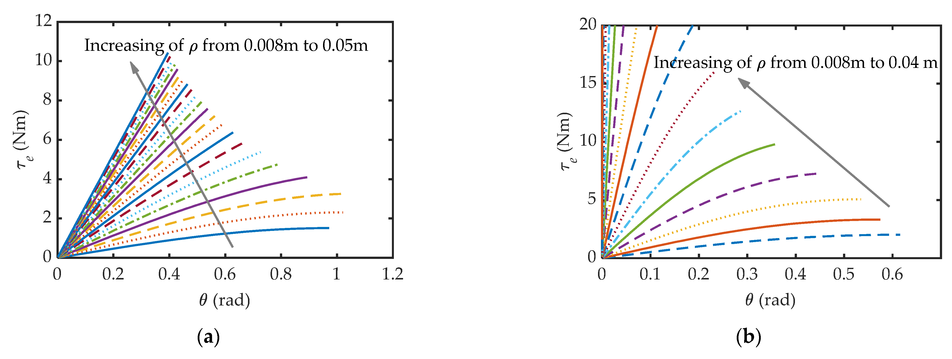
4.1. Characteristic Analysis of Stiffness Adjustment Module

There are two configurations by re-locate the position of the frame OB in the crank-slider mechanism online, as shown in Figure 4a (AB > OA) and Figure 4b (AB < OA).

Based on principles of virtual work, the output torque τ_e can be obtained as τ_e = τ_s(α)dα/dθ. τ_s(α) is the elastic torque of the spring with respect to the spring angular deflection α. Thus, the stiffness K can be described as,

$$K=\frac{d{\tau }_e}{d\theta }=k_s{\left(\frac{d\alpha }{d\theta }\right)}^2+{\tau }_s\left(\alpha \right)\frac{d^2\alpha }{d^2\theta }$$

(6)

where the transmission ratio (dα/dθ) is,

$$\frac{d\alpha }{d\theta }=\frac{\rho \cos \beta }{\left(OA\cos \alpha +\rho \cos \beta \mathrm{sign}(AB-OA)\right)}$$

where β indicates the angular displacement of the slider relative to OB in Figure 4.

According to Equation (6), it can be noted that: for the configuration I with AB > OA Figure 4a), the output stiffness K can be regulated with higher accuracy in a limited range (K < k_s) as dα/dθ < 1. Its output torque increases with an increasing of ρ, but is limited by the rated load of the spring (Figure 5a). For the configuration II with AB < OA (Figure 4b), dα/dθ can be tuned from zero to infinite by increasing the length of frame OB from zero to OA. As a result, the VSA can change the stiffness in a much broader range (from zero to infinity) even by using softer springs. In low ρ range (ρ ≤ 0.02 m), its output torque is limited by the rated load of the spring as in configuration I. With an increasing of ρ (ρ ≥ 0.022 m), the performance of the motors becomes the main constrained factor (Figure 5b). Due to the nonlinear characteristic of dα/dθ, there is nonlinear between output torque τ_e and deformation angle θ, especially in low ρ range. By reconfiguring the crank-slider mechanism online, the stiffness behavior can be changed to be compatible with different tasks requirements.

Benefitting from the concise static force relationship of the crank-slider mechanism (F_a, F_d in Figure 4), the mechanical property of stiffness adjustment corresponding to the two configurations can be expressed in a unified form as,

$$f(\rho ,\theta )=F_a/F_d=\tan \beta =OA\sin \theta /\left(sign(AB-OA)\rho +OA\cos \theta \right)$$

(7)

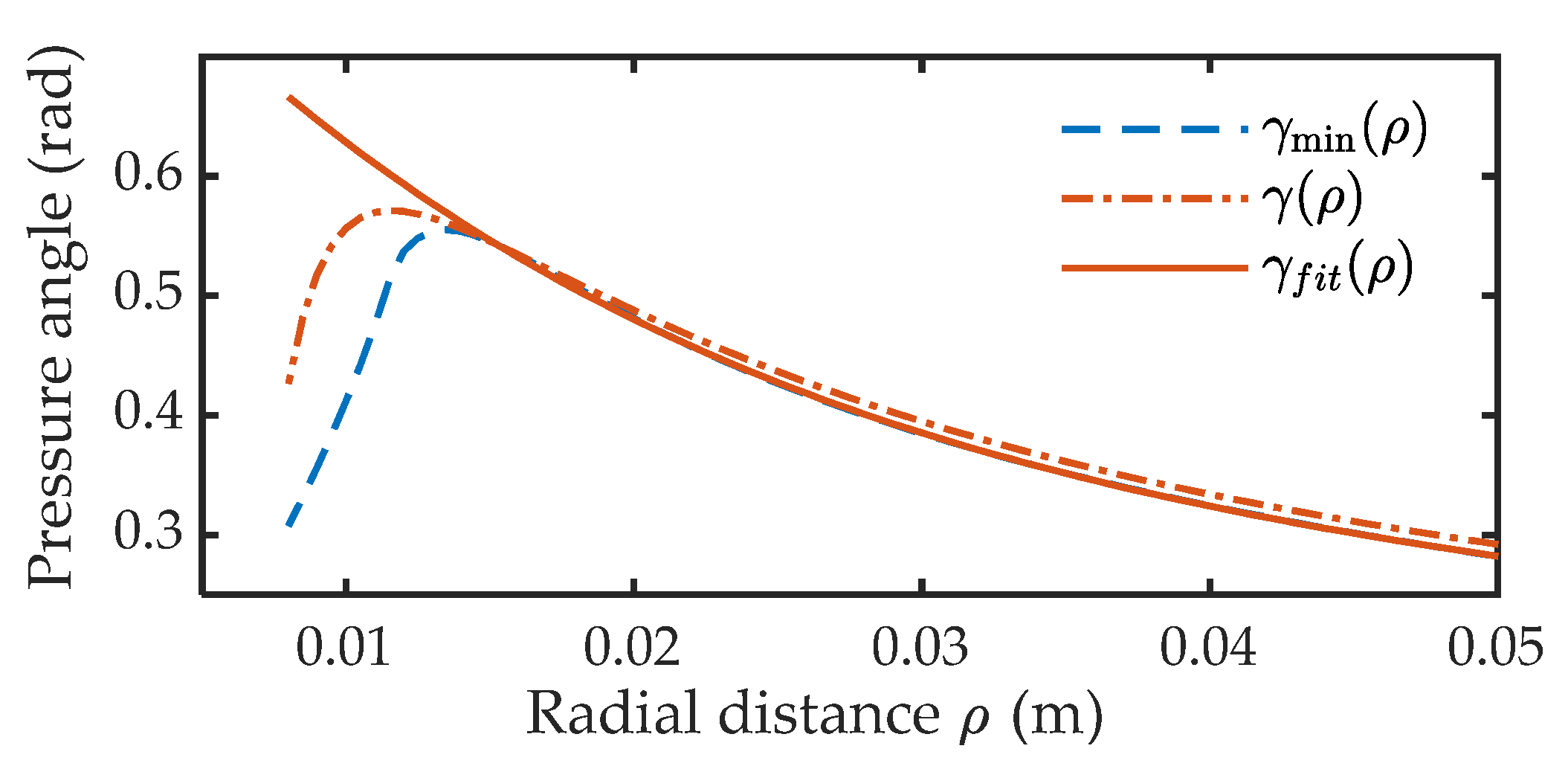
4.2. Numerical Synthesis of the Pressure Angle of the Cam Pitch Curve

4.2.1. Minimum Pressure Angle Constrained by Bearing’s Rated Load

There are two major factors that affect cam size: the range of the radial distance ρ and the pressure angle function γ (ρ). The former involves the output stiffness, and the latter relates to the load ratio. Optimal load ratio requires γ (ρ) to be minimized. It increases the forces on the follower bearings (F_M1, F_M2 in Figure 4b). Considering the specifications in Table 1, the constraint equations of the bearing’s rated load on γ (ρ) are as follows,

$$\{\begin{array}{l}{F}_{M1}={\tau }_e\left(1+\tan \beta \tan \gamma \left(\rho \right)\right){\rho }^{-1}/2\sin \gamma \left(\rho \right)\le \left[F_b\right]\\ \beta =\arcsin (a\sin \alpha {\rho }^{-1})\\ \theta =\beta +\alpha \mathrm{sign}(AB-OA)\\ {\tau }_e={\tau }_s\left(\alpha \right)d\alpha /d\theta \le {\tau }_o\end{array}$$

(8)

Taking both configurations into account, the numerical synthesis result of the minimum pressure angle is dashed (γ _min(ρ) in Figure 6). There appears an inflection point near ρ = 0.014 m on the curve. At the beginning of the curve (ρ < 0.014 m), a small γ _min (ρ) is allowed with a small τ_e, as the transmission ratio (dα/dθ) is very small. The dα/dθ increases greatly with the increasing of ρ and be the main factor of a remarkable increasing γ _min(ρ). After crossing the inflection point, the γ _min(ρ) decreases slowly similar to an inverse proportion graph, for that ρ ⁻¹ becomes the dominant factor.

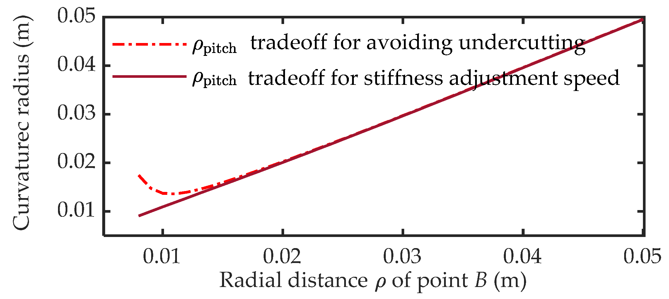
4.2.2. Tradeoff for Improving Stiffness Adjustment Speed Locally

According to Equation (1), the stiffness adjustment angle κ would be very big with an excessively small γ _min (ρ), when the ρ is in the low radial distance range (ρ < 0.014 m). In other words, the stiffness adjustment speed would be very slow in this region. In fact, the output torque can be supported by a single motor as the stiffness is very low in this range. So, there can be a reasonable tradeoff between the load ratio and the stiffness adjustment speed by appropriately reducing the ϕ for a bigger pressure angle. The pressure angle of cam pitch curve can be adjusted locally by adding a correction function according to the design requirement. In this paper, the calculation data by Equation (8) are directly fitted in fourth-order (solid in Figure 6), after excluding the data in ρ < 0.014 m. The numerical synthesis formula of the cam pitch curve is,

$${\gamma }_{fit}(\rho )=20830{\rho }^4-5303{\rho }^3+531.5{\rho }^2-27.36\rho +0.854$$

(9)

4.2.3. Tradeoff for Avoiding Undercutting

The curvature radius of the pitch curve on the cam is a mathematical function of γ (ρ), ρ. It can be written as,

$${\rho }_{\mathrm{pitch}}=\frac{\rho {\left[1+{\tan }^2\gamma \left(\rho \right)\right]}^{3/2}}{\left|{\tan }^2\gamma -\rho {\gamma }^{\prime }\left(\rho \right)\tan \gamma \left(\rho \right){\sec }^2\gamma \left(\rho \right)+1\right|}$$

(10)

Substituting Equation (9) into Equation (10), we can obtain the curvature radius shown in Figure 7 (solid). The minimum radius of the curvature (9 mm) is smaller than the radius of the follower bearing (9.5 mm). The undercutting problem occurs. A common choice is to locally reduce the pressure angle γ (ρ) in the low range (ρ < 0.014 m) with little influence on the other range. The correction term added to Equation (9) is,

$${\gamma }_c(\rho )=a_c+b_c{({\rho }_{\min }/\rho )}^{n_c}$$

(11)

By adjusting the coefficients n_c and b_c, the correction term can effectively reduce the pressure angle to solve the undercutting problem when ρ is small. Its influence decays rapidly with an increasing of ρ. Furtherly, the normal coefficient a_c is used to repair the influence on the large radial distance range. To avoid the correction term ${\gamma }_c\left(\mathsf{\rho }\right)$ exceeding the limitation of the rated load of the cam follower, the ${\gamma }_c\left(\mathsf{\rho }\right)$ should meet the following equations:

$$\{\begin{array}{l}{\gamma }_c(\rho )+{\gamma }_{fit}(\rho )\ge {\gamma }_{\min }(\rho )\\ {\rho }_{\mathrm{pitch}}\ge D/2\end{array}$$

(12)

Setting a_c = 0.01, b_c = −0.25, n_c = 5 by enumeration method, the final pressure angle is graphed in Figure 6 (dotted) and the corresponding curvature radius is graphed in Figure 7 (dotted) with a minimum value of 13.6 mm. This now has become an acceptable cam, because both the minimum curvature radius, bearing rated load, load ratio and stiffness adjustment speed are compromised well. The pressure angle function of the pitch curve on the finally fabricated cam is

$$\gamma (\rho )=20830{\rho }^4-5303{\rho }^3+531.5{\rho }^2-27.36\rho +0.864-0.25{({\rho }_{\min }/\rho )}^5$$

(13)

4.3. Comparative Analysis of Design Result

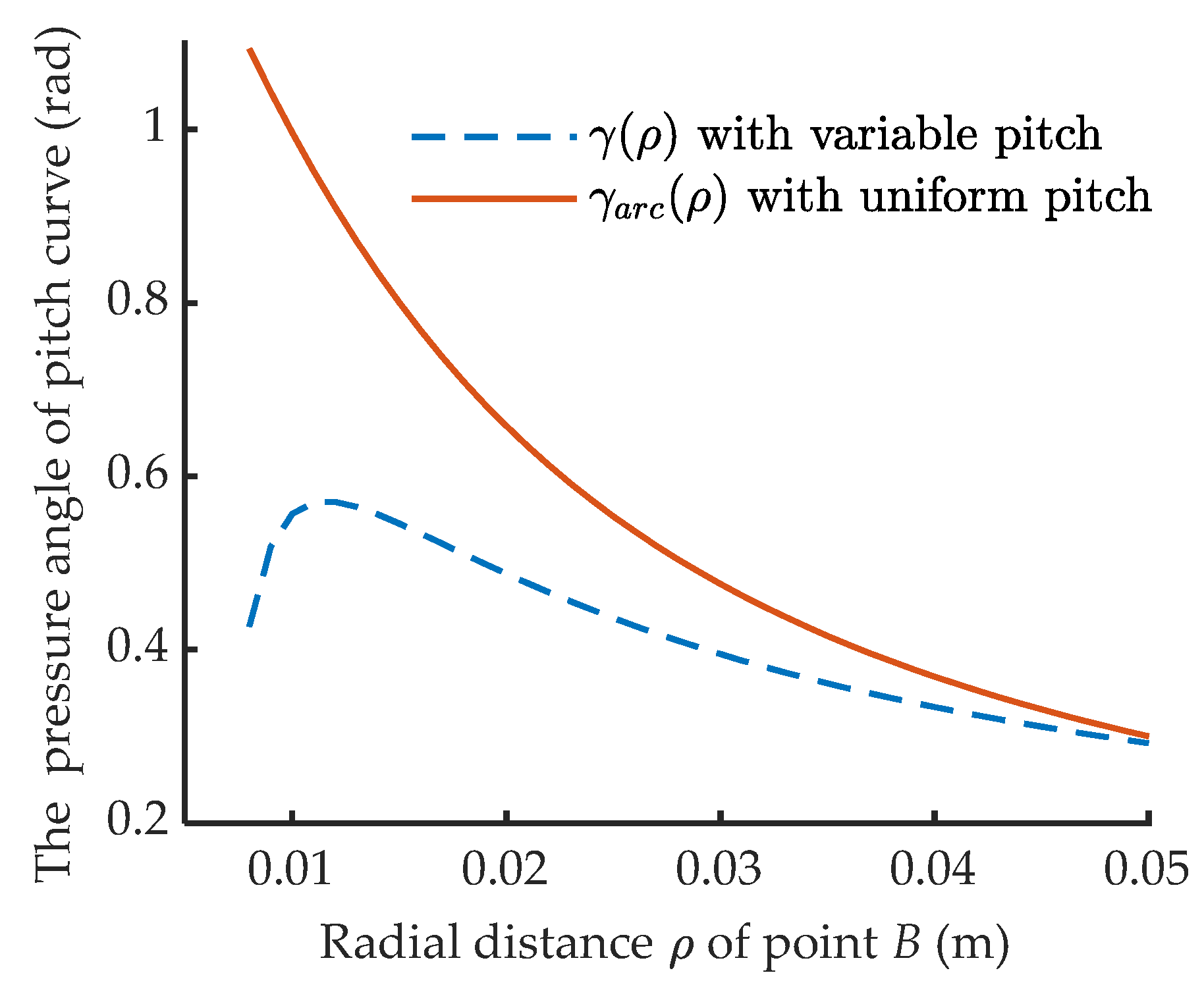
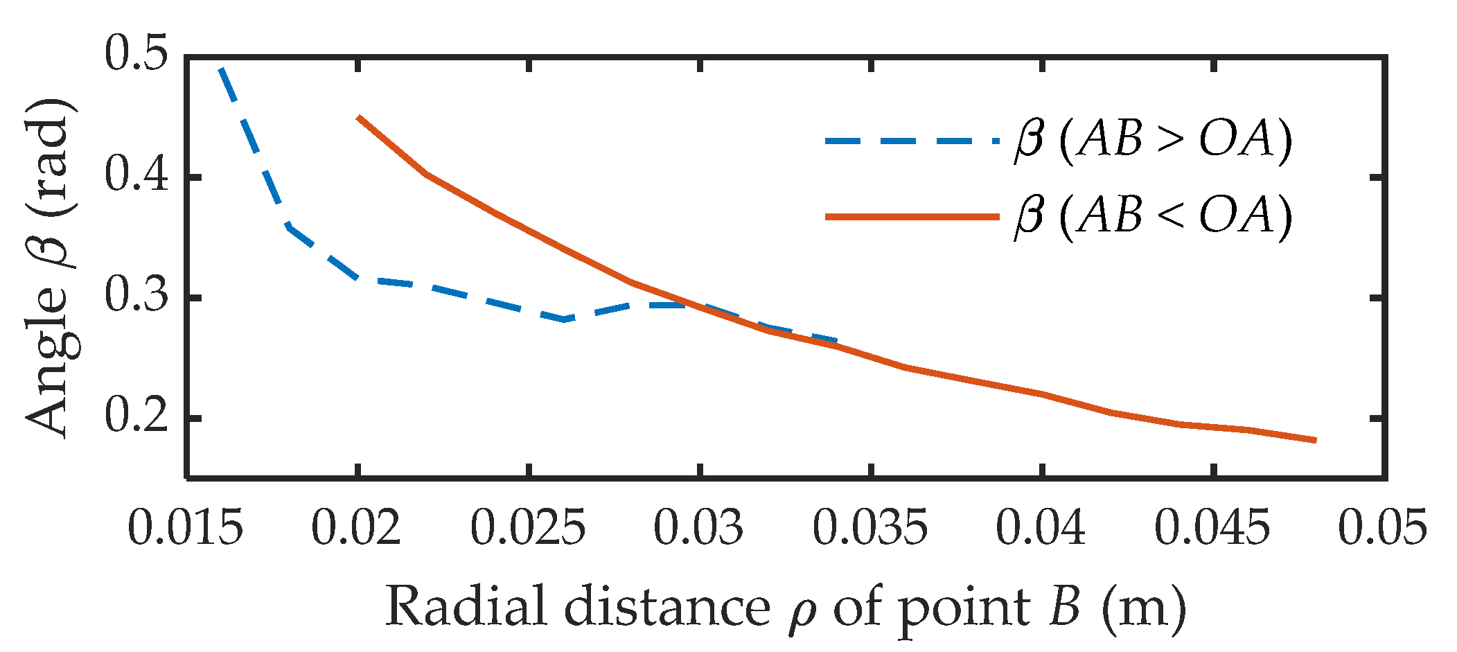
4.3.1. Analysis of Pressure Angle

Substituting Equation (13) into Equation (1), the variable-pitch curve is dashed in Figure 8. Its shape is similar to that of Archimedean spiral. However, the latter is strongly constrained with only two parameters (initial radial distance and uniform pitch), which makes it difficult to carry out the above tradeoff design. For more specific comparison, the formula of Archimedes curve accorded with the same constraints in the paper is proposed as the solid line in Figure 8, and expressed by,

$${\rho }_{arc}=0.008+0.015\kappa$$

(14)

The proposed pitch curve deviates from the Archimedean spiral with a smaller pressure angle γ (ρ) (Figure 9). It is the concrete embodiment of cam curve tradeoff design by locally adjusting the pressure angle.

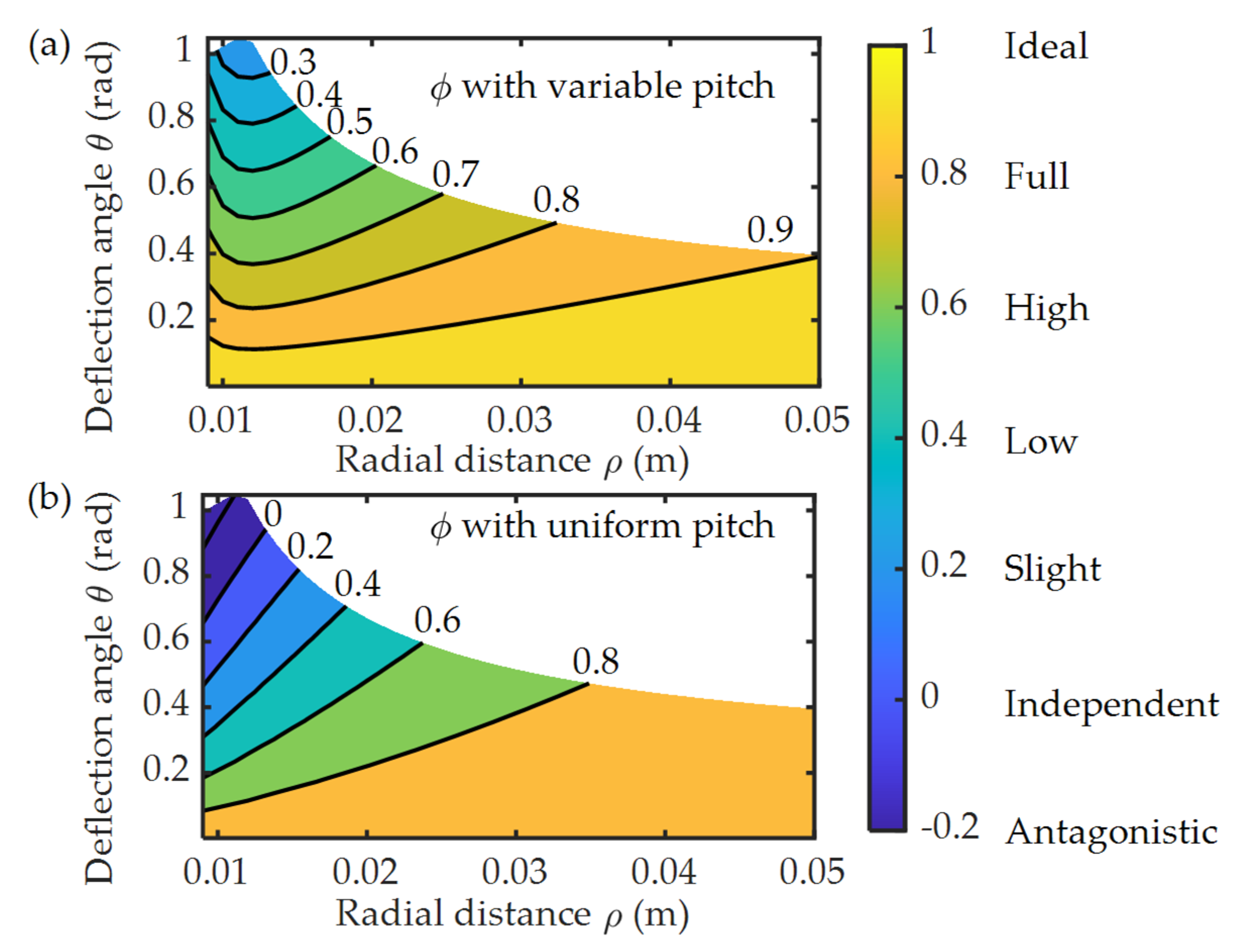
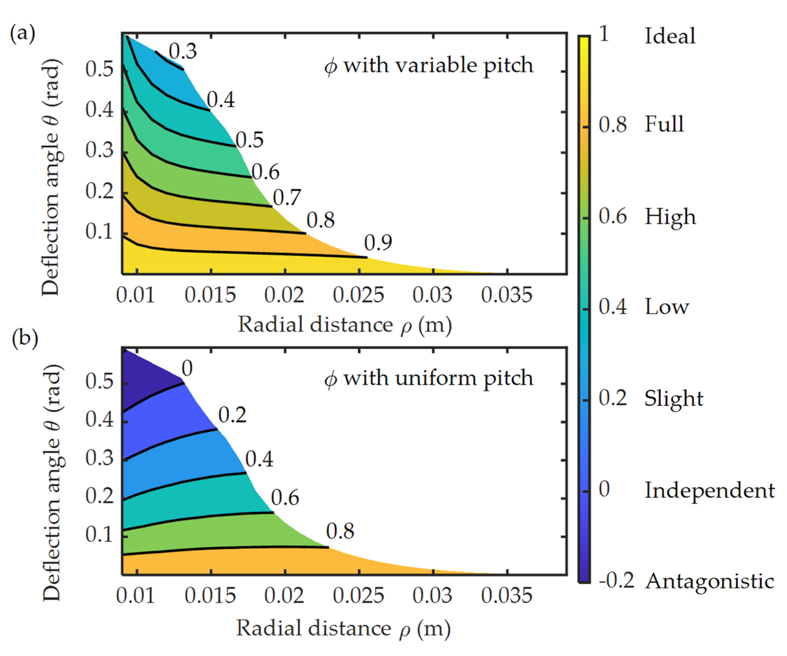
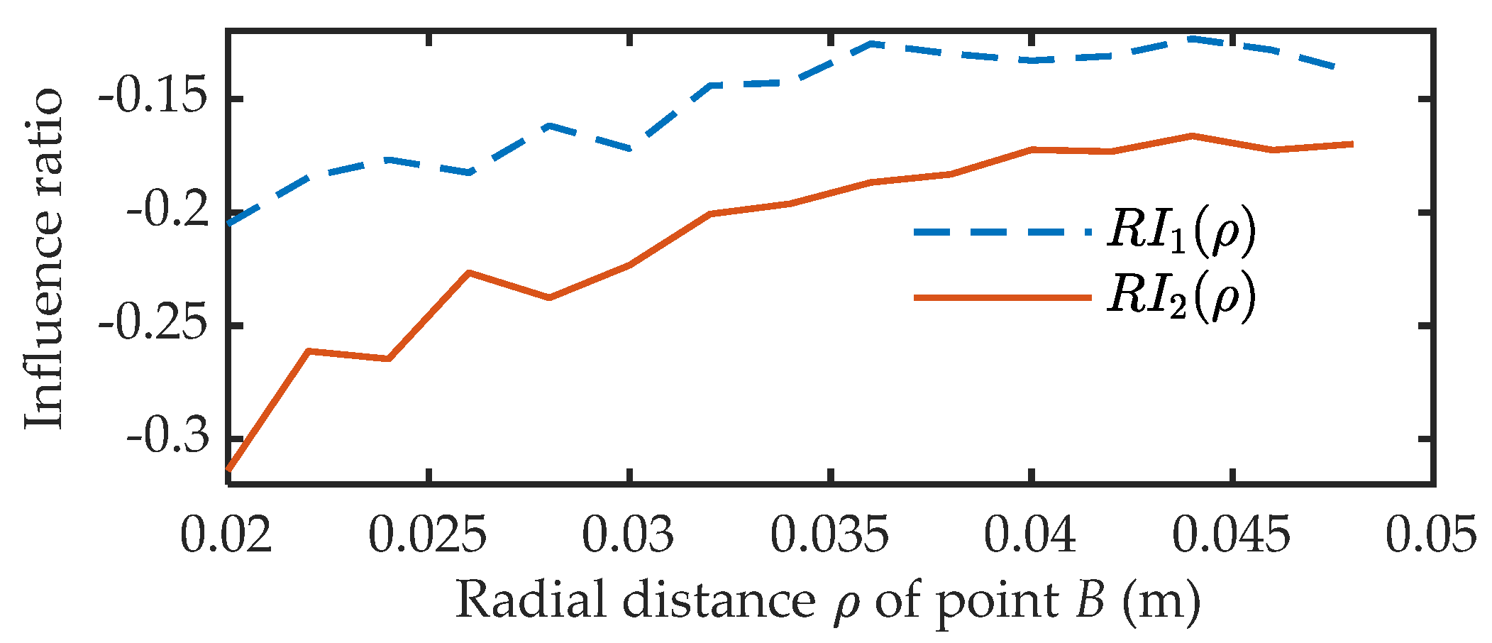
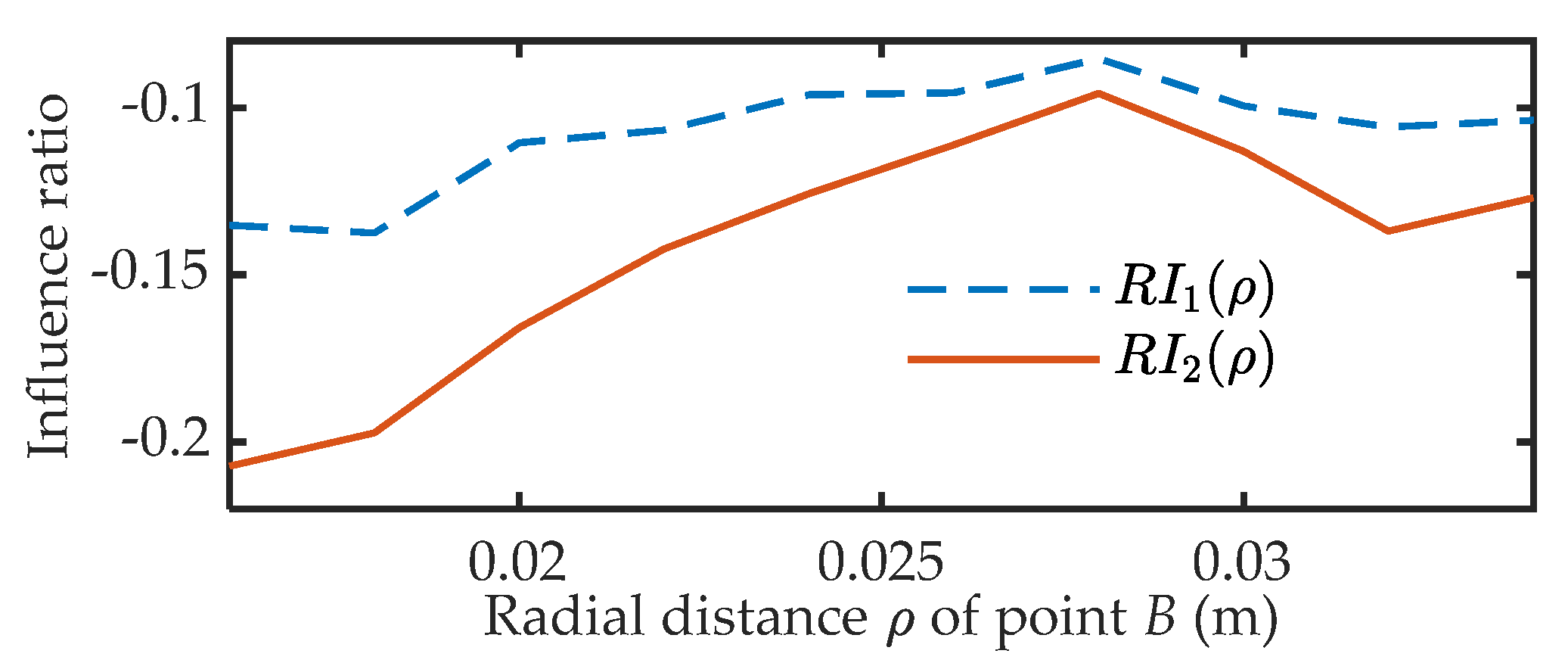
4.3.2. Design Results Analysis of the Load Ratio

According to the specifications in Table 1, the load ratio design results of the two configurations with different cams curve are shown by the color contour in Figure 10 (configuration I, AB > OA) and Figure 11 (configuration II, AB < OA).

The color depth indicates the value of the load ratio ϕ. We furtherly classify the workspace (color area) with different helping levels. They are, respectively, ideal area (ϕ = 1), full area (0.8 $\le$ ϕ <1), high area (0.6 $\le$ ϕ < 0.8), low area (0.4 $\le$ ϕ < 0.6), slight area (0 < ϕ < 0.4), independent area (ϕ = 0) and antagonistic area (ϕ < 0).

From the aspect of the load ratio, the helping mode with variable pitch curve shows a higher level over than that of the uniform pitch curve. The proportion of the area with different level over the whole workspace can be used to evaluate the difference of their load ratio. In configuration I, the proportion of the full area with the uniform-pitch cam (Figure 10b) slightly less than that with variable-pitch cam (Figure 10a), when the ρ is near to 0.05 m. However, as the ρ decreases, the difference rapidly enlarges, and the former even entries into the antagonistic area. This trend is more obvious in configuration II (Figure 11). These phenomena can be clearly explained by the variables in Equations (4) and (7), i.e., γ (ρ) and β. The γ (ρ) of the uniform-pitch cam is equal to that of the variable-pitch cam at ρ = 0.05 m. However, the former is inevitably increasing when the ρ decreases, as the curve formula in Equation (14) has been decided by the ρ range and bearing rated load. However, for the variable-pitch curve, a good tradeoff can be allowed. Its pressure angle can be arbitrarily adjusted and be well fit with the mechanical property of the stiffness adjustment module. This results a smaller γ (ρ) and a larger ϕ. As a results, the antagonistic area shrinks into the slight area and the other helping levels occupy a higher proportion. So, the dual motors can work against the output load together in the same direction with a closer amount. This phenomenon in configuration II will be more outstanding than that of configuration I, as the former has a bigger f (ρ,θ). To optimize the load ratio furtherly, the follows methods can be taken:

• Changing cam followers with higher rated load [F_b]. With the same constraints in this paper, a smaller pressure angle γ (ρ) can be realized according to the rated load constraint equations in Equation (8).
• Redesigning the variable stiffness module for a smaller f (ρ,θ). In this case, the helping level with higher value can occupy a bigger area proportion, as shown in (Figure 10a and Figure 11a).

5. Load Ratio Validation by Experiment

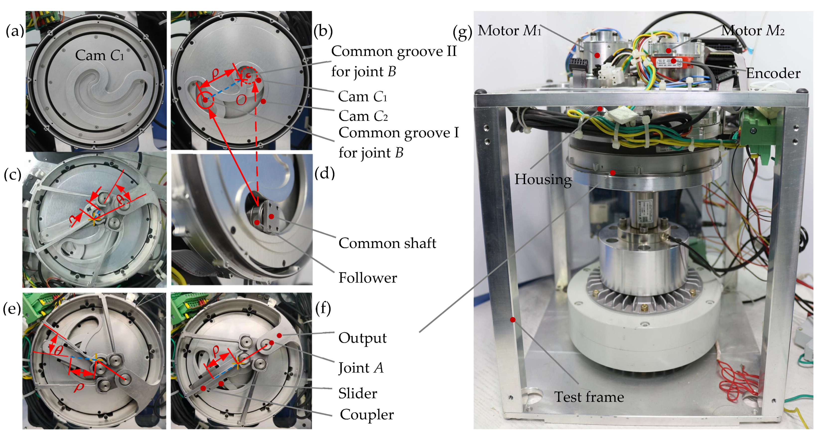
5.1. Reconfigurable Prototype and Test Platform

The symmetrical cams C₁ and C₂ in Figure 12a,b were machined according the pitch curve function in Equation (13). Corresponding to the two configurations in Figure 4, there are two common grooves with a phase difference of 180°. The VSA configuration can be initialized by locating the joint B to common grooves I or II in Figure 12b. The former corresponds to configuration I in Figure 4a, and the latter to configuration II in Figure 4b. Joint B consists of two follower bearings and a common shaft (Figure 12d). Meanwhile, the common shaft is fixed on the slider, which can move along the coupler (Figure 12f). By synchronous control of the dual cams, the desired θ can be obtained. A special case is shown in Figure 12c, in which the θ can be load to 2π rad with output end fixed and a low ρ value (such as ρ = 8 mm). In this approach, the VSA can be switched online from configuration II to configuration I without overloading the spring. Its inverse transform can be implemented in the same way. By cams differential control, the goal ρ for stiffness adjustment can be set. Figure 12e,f are the deformed and undeformed cases of configuration I. The value of ρ and θ can be calculated according to the motors M₁ and M₂ encoders, as both the housing and the output link are fixed with the test frame (Figure 12g).

5.2. Dealing Method of Current Data with Bang-Bang Friction

In this section, the torques exerted on the cams are estimated by the frictionless driving current of the dual motors under different ρ and θ. The motors torque τ_m1 and τ_m2, cams driving torque T_M 1(ρ,θ), T_M 2(ρ,θ) and external load τ_e meet the following static equilibrium equations:

$$\{\begin{array}{l}{T}_{M1}\left(\rho ,\theta \right)={\tau }_{m1}\left(N_1,I_1\left(\rho ,\theta \right),{\eta }_1,i_1\right)+{\tau }_{f1}\mathrm{sign}({\dot{q}}_1)=\left(1-\tan \left(\beta (\rho ,\theta )\right)\tan \gamma (\rho )\right){\tau }_e/2\\ T_{M2}\left(\rho ,\theta \right)={\tau }_{m2}\left(N_2,I_2\left(\rho ,\theta \right),{\eta }_2,i_2\right)+{\tau }_{f2}\mathrm{sign}({\dot{q}}_2)=\left(1+\tan \left(\beta (\rho ,\theta )\right)\tan \gamma (\rho )\right){\tau }_e/2\end{array}$$

(15)

where I₁(ρ,θ) and I₂(ρ,θ) indicates the current of the dual motors, τ_f1 and τ_f2 denote the friction of the two kinematic chains in Figure 2b, η₁ and η₂ are the efficiency, i₁ and i₂ are the gear train ratio, N₁ and N₂ are the torque constant. i₁, i₂, N₁, N₂ are corresponding to the parameters in Section 2.

Under external load, the motor’s relative motion trends toward its absolute equilibrium position by the position servo control. This trend decides the friction direction and can be mathematically indicated by the sign of ${\dot{q}}_i$ (i = 1,2), where q_i is the motor position. There are three cases according to the sign of ${\dot{q}}_i$ and the toggle between these cases would have great perturbation on the currents of the dual motors.

For the case of ${\dot{q}}_i$> 0, the friction helps to work against the external load. Then this type of current can be called positive-friction current and is expressed as,

$$I_i^P\left(\rho ,\theta \right)=\left(T_{Mi}\left(\rho ,\theta \right)-{\tau }_{fi}\right)/N_i{\eta }_i{i}_i$$

(16)

In a likewise fashion, a negative-friction current is expressed as,

$$I_i^N\left(\rho ,\theta \right)=\left(T_{Mi}\left(\rho ,\theta \right)+{\tau }_{fi}\right)/N_i{\eta }_i{i}_i$$

(17)

For the last case of ${\dot{q}}_i$ = 0, it is the frictionless current. The current, in this case, is just what we need to estimate the cams driving torque T_M1(ρ,θ), T_M2(ρ,θ) for load ratio calculation. We express this frictionless current as,

$$I_i^O\left(\rho ,\theta \right)=T_{Mi}\left(\rho ,\theta \right)/N_i{\eta }_i{i}_i$$

(18)

An example of the above cases is shown in Figure 13 and Figure 14, in which ρ = 0.048 m and θ varies from −0.4 rad~0 rad. The positive-friction current and negative-friction current are, respectively, marked with Δ and ∗, apart from the frictionless current circled with an ellipse. Most of the current data jump back and forth between the former two types (blue curves in Figure 13 and Figure 14). It represents that the friction torque direction continues to switch. An obvious current stratification can be observed and it is the basic of frictionless current estimation.

The frictionless current data are very few, as frictionless state is unstable. So, the frictionless current for dual cams should be estimated by,

$$I_i^o(\rho ,\theta )=\left(I_i^p(\rho ,\theta )+I_i^n(\rho ,\theta )\right)/2$$

(19)

where $I_i^{ p}(\rho ,\theta )$ and $I_i^{ n}(\rho ,\theta )$ are the fitted results of the positive-friction current and negative-friction current data, respectively. They are described by,

$$\left[\begin{array}{l}{I}_1^p(\rho ,\theta )\\ I_1^n(\rho ,\theta )\\ I_2^p(\rho ,\theta )\\ I_2^n(\rho ,\theta )\end{array}\right]=\left[\begin{array}{cccc}{a}_{11}^{\rho }& a_{12}^{\rho }& a_{13}^{\rho }& a_{14}^{\rho }\\ a_{21}^{\rho }& a_{22}^{\rho }& a_{23}^{\rho }& a_{24}^{\rho }\\ a_{31}^{\rho }& a_{32}^{\rho }& a_{33}^{\rho }& a_{34}^{\rho }\\ a_{41}^{\rho }& a_{42}^{\rho }& a_{43}^{\rho }& a_{44}^{\rho }\end{array}\right]\left[\begin{array}{l}{\theta }^3\\ {\theta }^2\\ {\theta }^1\\ 1\end{array}\right]$$

(20)

Noting that the two kinematic chains have the same transmission structure and similar gear ratio, we can approximately set η₁=η₂. Then, the testing load ratio can be put into a more convenient form as,

$${\varphi }_{\mathrm{test}}=\frac{N_1{i}_1{I}_1^o(\rho ,\theta )}{N_2{i}_2{I}_2^o(\rho ,\theta )}$$

(21)

Substituting Equation (7) into Equation (4), the theory load ratio can be calculated by,

$${\varphi }_{\mathrm{theory}}=\frac{1-\tan \left(\beta (\rho ,\theta )\right)\tan \gamma (\rho )}{1+\tan \left(\beta (\rho ,\theta )\right)\tan \gamma (\rho )}$$

(22)

Again, the current data in Figure 13 and Figure 14 are utilized to illustrate the data dealing process. The results are shown in Figure 15 and Figure 16, in which the $I_i^{ p}(\rho ,\theta )$ is dashed and the $I_i^{ n}(\rho ,\theta )$ dotted. The estimation curve of the frictionless current is the solid in the middle according to Equation (19). The testing load ratio in Equation (21) is ϕ_test = 0.85 with θ = −0.4 rad. The related variables in Equation (22) are β (ρ,θ) = 0.18 rad, γ (ρ) = 0.3 rad, which can be obtained with θ = −0.4 rad and ρ = 0.048 m according to Figure 4a and Equation (13). This leads to ϕ_theory = 0.9. The test result is 5.6% smaller than its theory value.

5.3. Results of the Experiment

5.3.1. Measurement Range Choosing

The following two methods are taken to ensure the accuracy and validity of the load ratio estimation. Firstly, the measurement range of ρ is comprehensively considered. In Equation (19), the paper defaults that the friction of the kinematic chain remains constant. The friction mainly comes from the harmonic gear. In fact, it shows a periodic fluctuation due to manufacturing reasons. This fluctuation significantly contributes to the change of the current gap (between the dashed line and dotted line), as shown in Figure 15 and Figure 16. This will have a significant impact on the accuracy of the evaluation results, especially when the current is small. So, the radical distance with low ϕ should be excluded, as the current of some motor will be very small in this case. We set the range to be ϕ > 0.7, and the ρ range can be preliminarily selected according to Figure 10a and Figure 11a. However, for estimation comparison and analysis, the measurement range should be appropriately broadened. Another important factor is stiffness. If the stiffness is too high, it is hard to gain a practical and accurate β for Equation (22), especially when the ρ is close to 0.04 m in configuration II. So, in the configuration I, the measurement range is ρ ∈ [0.02 m, 0.048 m]; in the configuration II, it is [0.016 m, 0.034 m].

Secondly, the deformation angle θ is loaded to its limit for a higher motor current. It is constrained by the spring deformation capacity or the nominal torque of the motor. In Equation (21), we set θ as maximum deflection angle gained in the test, and not all the points Figure 10a and Figure 11a will be estimated for the ρ range chosen.

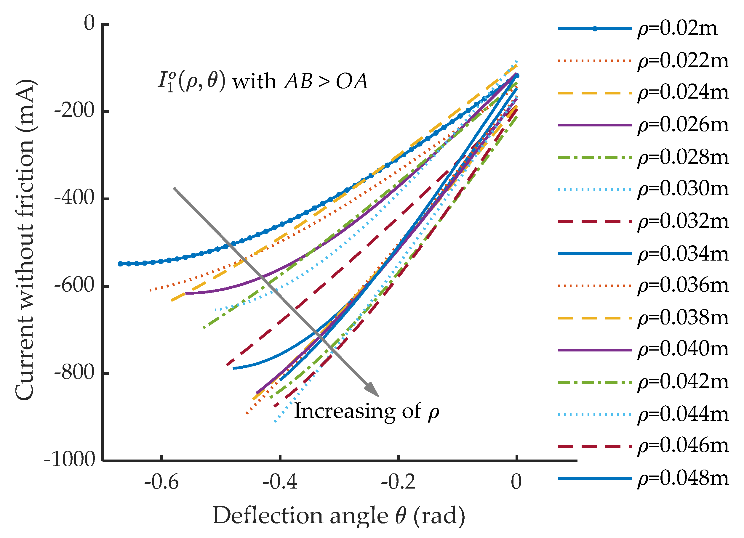
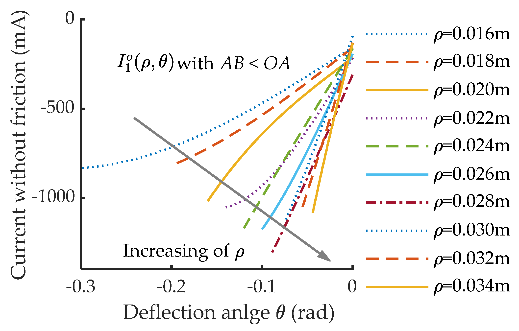
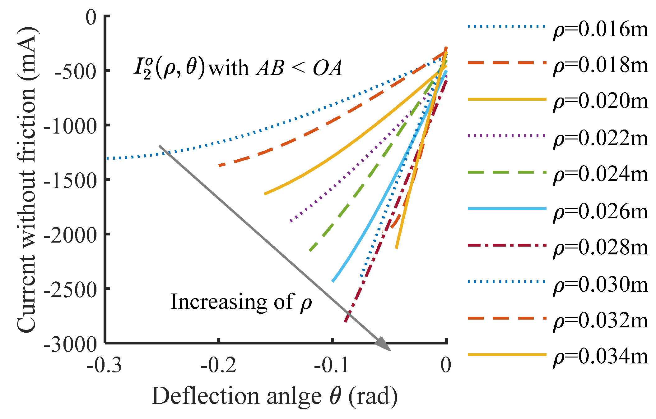
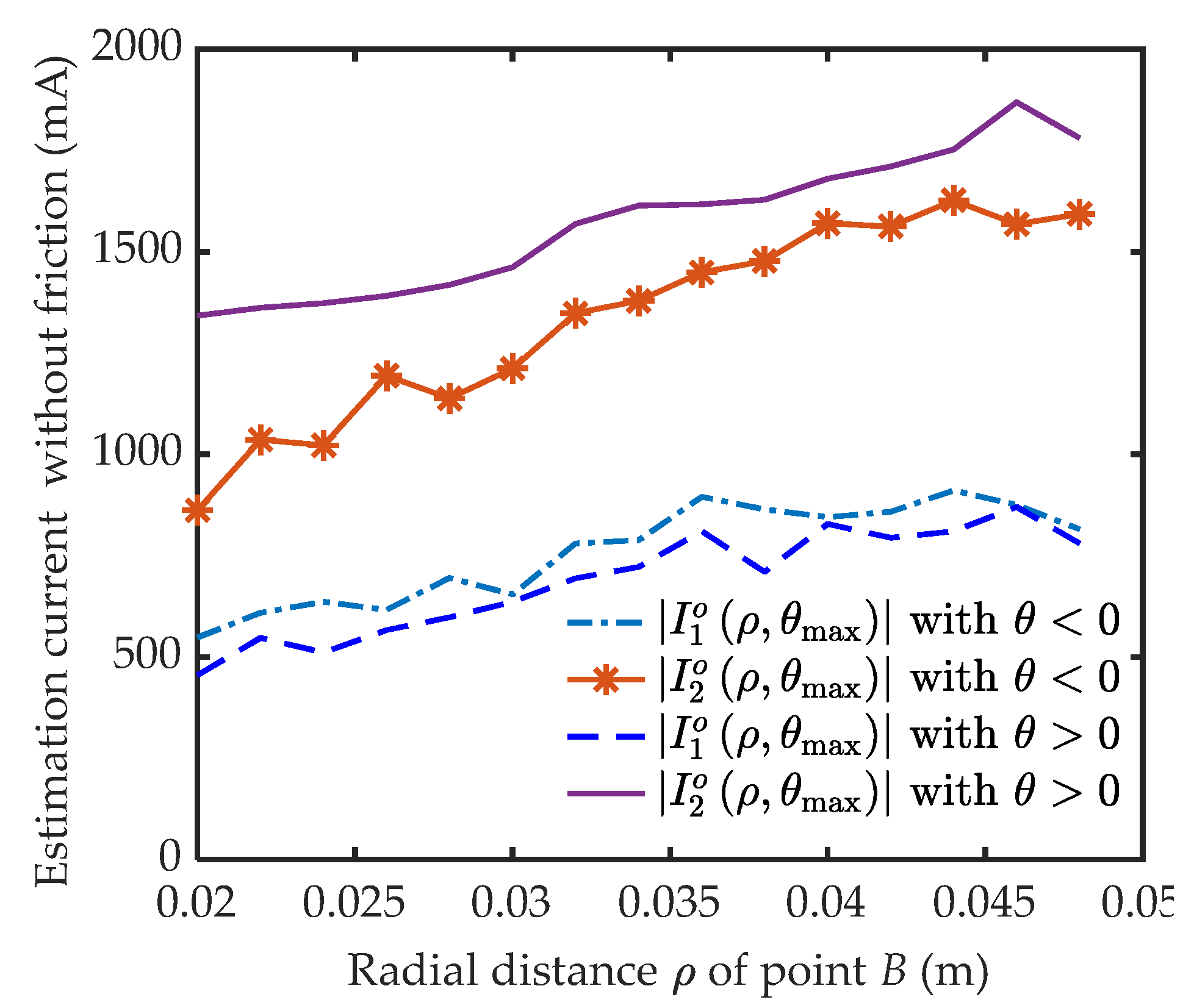
5.3.2. Frictionless Drive Current Estimation for the Dual Cams

The current dealing approach in Section 5.2 is applied to the whole measurement range with a negative deflection firstly (θ < 0). For configuration I, the estimation results of frictionless current for cams C₁ and C₂ are plot in Figure 17 and Figure 18. The ρ varies in the arrowed direction with a step of 0.002 m. The frictionless currents for both cams changes with a highly convergent trend in the same direction, as the deflection angle increases in the whole measurement range. Their current magnitude difference is due to the difference of torque constant and gear ratio in their kinematic chains.

The estimation results of configuration II exhibit a similar feature, as shown in Figure 19 and Figure 20. The difference is that deflection-current curves in the large ρ value quickly become high-slope curves due to their broader stiffness. These results prove that the dual motors are always in helping mode in the measured workspace with both two configurations.

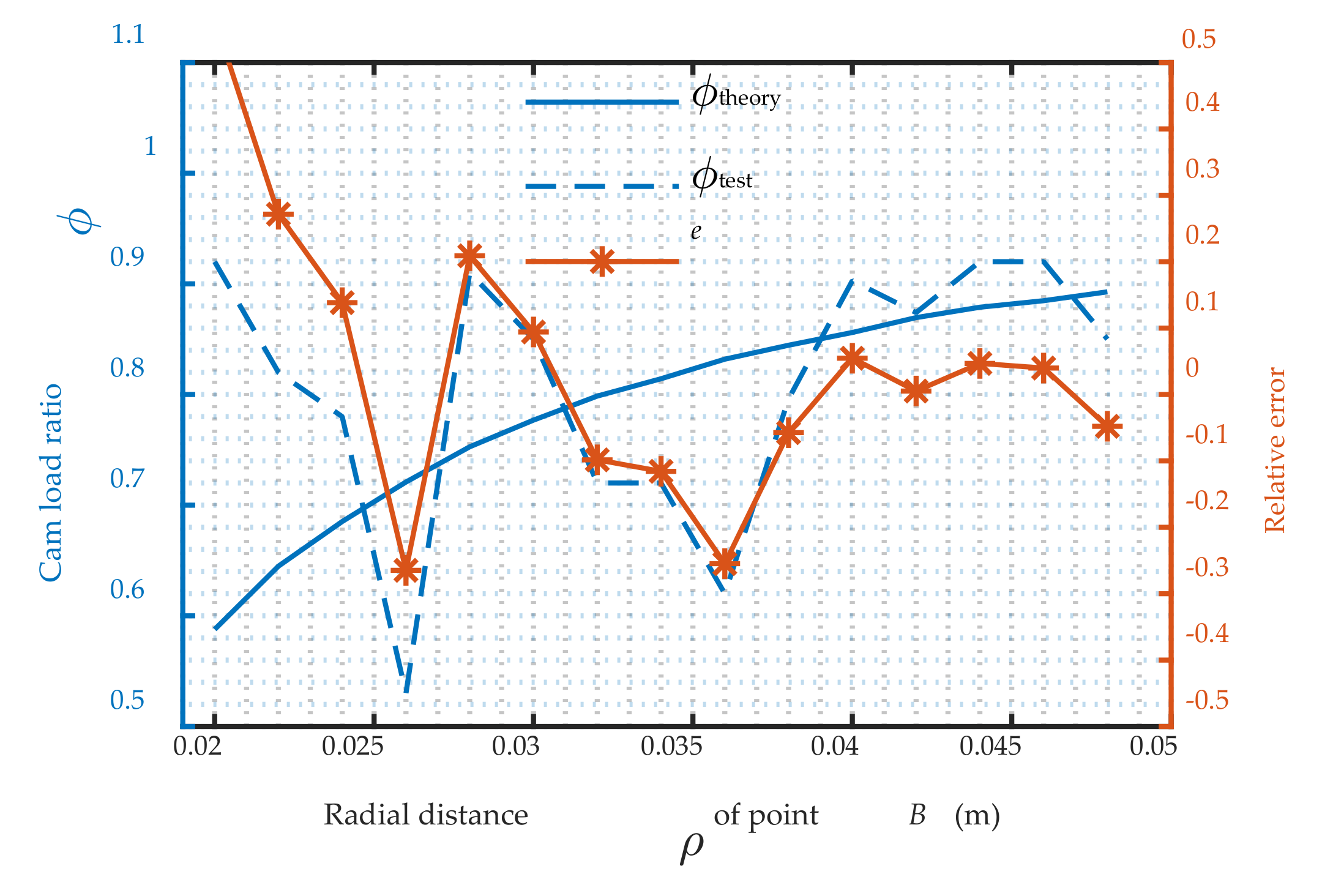
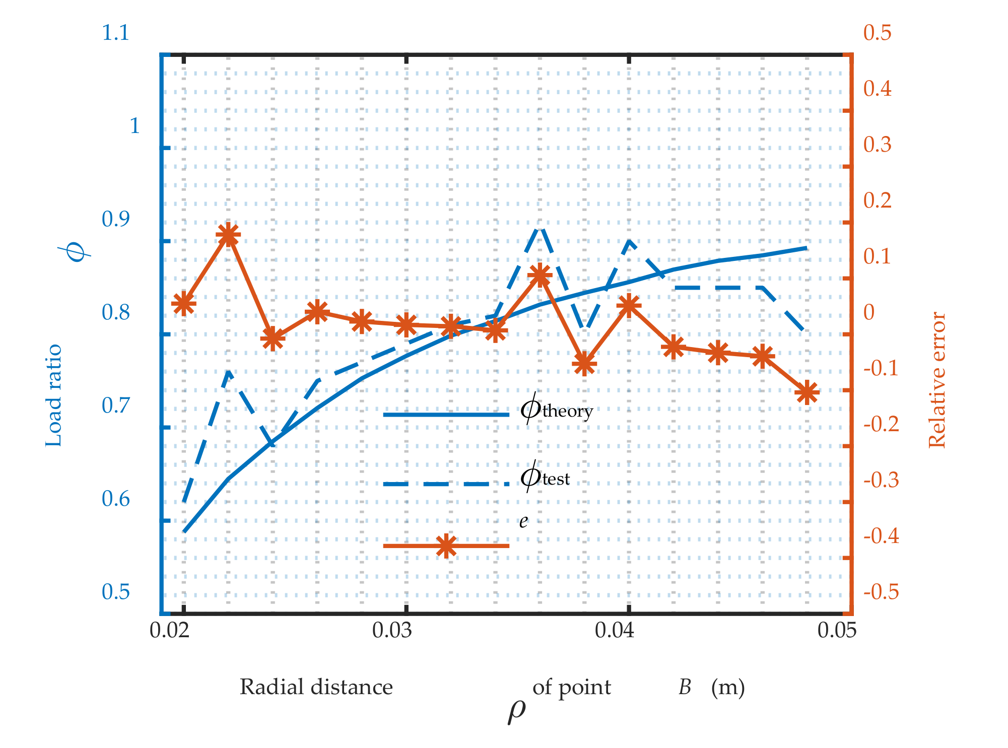
5.3.3. Estimation Results of Load Ratio

For the two configurations, both the maximum deflection angle θ can be obtained in the above estimation curves (Figure 17, Figure 18, Figure 19 and Figure 20). Going back to Equation (21) with the maximum θ, the testing load ratios can be resulted, as shown in Figure 21 and Figure 22 (ϕ_test, dashed). The former is the case for configuration I and the later for configuration II. The maximum β (ρ,θ) can be easily achieved according to the geometry relationship in Figure 4, as the radial distance ρ and maximum deflection angle θ are known. The corresponding theory load ratio are also graphed in Figure 21 and Figure 22 (ϕ_theory, solid) according to Equation (22). The relative errors are marked by * (e = (ϕ_test − ϕ_theory)/ ϕ_theory, asterisked in Figure 21 and Figure 22). For configuration I, the relative error is nearly to 60% with ρ = 0.02 m. After that, the error converges into 30% and partially into 10% as the ρ increases from 0.038 m to 0.048 m. For another configuration, the error fluctuates within 30%.

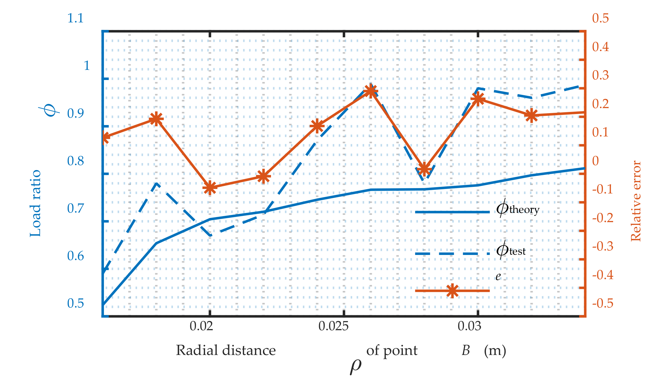
5.3.4. Error Analysis

The estimation results of the load ratio are not satisfactory, as only part of the relative error is within 10%. The error factors include: cam manufacture accuracy, motor position accuracy, motor current noise, simplification of transmission efficiency (i₁≈i₂), friction fluctuation and insufficient stiffness of the kinematic chain. Modern industrial manufacturing capacity and mature motor control technology make the first four factors have little influence on the test accuracy of load ratio. So, the error mainly comes from the friction variation and stiffness weakening by the kinematic chains.

The stiffness weakening phenomenon will be relatively noticeable in the high stiffness but slight in the low stiffness, as the variable stiffness module is connected in series with the kinematic chains. This can be guessed by the curve comparison of angle β, which has a very significant impact on the calculation of ϕ_theory. In configuration I, the maximum output stiffness is limited by the spring. So, the angle β of this case is smoothly decreased as the influence of the K_c can be ignored (solid line in Figure 23). However, in configuration II, the output stiffness can be very high, even be rigid. It can be reckoned the output stiffness must be over the chain stiffness after crossing some point. In this case, the output stiffness will be weakened seriously. It will result in a bigger β than the practical value. Therefore, there is a distortion on the β-ρ curve after the ρ cross 0.025 m (dashed line in Figure 23). We can draw a conclusion that the stiffness weakening contributes mostly to the error of configuration II with large ρ, i.e., in high stiffness region.

For quantitative influence analysis of friction fluctuation, the variation amplitude of the current gap is defined by ${DI}_i^{ n}(\rho )=m$ax ${(I}_i^{ n}(\rho ,\theta {)-I}_i^{ p}(\rho ,\theta \left)\right)$, i = 1,2. It can be seen as a motor current response to the friction variation. Influence ratio is defined as the response current over the frictionless current: ${RI}_i^{ n}\left(\rho \right)$= ${DI}_i^{ n}\left(\rho \right)$/$I_i^{ o}(\rho ,\theta \max )$, i = 1,2. The results are shown in Figure 24 and Figure 25. It can be observed that the influence of friction fluctuation put a bigger weight on the frictionless driving current of motor M₂ than that of motor M₁, especially in configuration I with a small ρ. The reason is that the torque constant and the gear ratio of motor M₂ are smaller than that of motor M₁. Correspondingly, the relative error e is very high in this interval. As the ρ increases, the output torque and motor current increase synchronous. This leads to a decay of the influence ratio. The relative error also decreases synchronously, as shown in Figure 21. However, it is not the case for the configuration II, as the chain stiffness weakening becomes the dominant factor.

According to the above error analysis conclusion, increasing the frictionless driving current of motor M₂ is expected reduce the influence ratio and the testing error. Based on this, the deflection direction is adjusted from negative to positive, as there is T_M2 > T_M1. The experiment is only performed in configuration I to avoid the weaking influence of chain stiffness. In Figure 26, the frictionless drive current for the dual cams with maximum deflection angle are plot in absolute values for comparison. The current for cams C₁ and C₂ with negative deflection direction is marked by ‘|$I_1^{ o}(\rho ,\theta \max )$| with θ < 0′ and ‘|$I_2^{ o}(\rho ,\theta \max )$| with θ < 0′, respectively, and the opposite are expressed by ‘|$I_1^{ o}(\rho ,\mathsf{\theta }\max )$| with θ > 0′ and ‘|$I_2^{ o}(\rho ,\theta \max )$| with θ > 0′. Compared with case of θ < 0, the current of motor M₂ increases by a big margin when the ρ is in low range with θ > 0. This margin decreases as the ϕ increases with an increasing of ρ. The variation margin is relatively small for cam C₁, as its gear ratio and torque constant are larger. It can be noted that the relative error converges into 10% quickly as expected (Figure 27). In the positive deflection direction, the result effectively testifies the correctness of load ratio design.

6. Conclusions

This paper presents a novel variable stiffness actuator (VSA) for a higher-level helping mode. The actuator mainly involves a variable-stiffness module based on a spring-balanced crank-slider mechanism and an actuation module based on dual differential cams with variable pitch curves. The two modules are connected by the non-center node of the frame. On this common node, the stiffness adjustment is realized by changing the transmission ratio of the deformation between the spring and the VSA, with a variable frame as the input link of the variable stiffness module. At the same time, the dual motors work against the external load together with a close amount.

The innovation of the proposed VSA is how the cam pitch curve is realized for optimal load distribution. A cam curve synthetic method has been presented, considering the pressure angle of the pitch curve, load distribution, stiffness adjustment speed, cam followers local load, the mechanical property of stiffness adjustment, and cam undercutting. The method shows that the smaller the pressure angle of pitch curve is, the closer the load ratio is to 1. It is at the cost of increasing the local load of the cam follower and decreasing the stiffness adjustment speed.

Furtherly, the pitch curve is synthesized after a reasonable trade-off. The actuator obtains a favorable load distribution in the whole workspace. In the fabricated prototype, motor current stratification caused by unstable friction direction has been clearly observed. The design result of the load distribution was effectively verified by frictionless current estimation after the main error factors were weakened, as the relative error converges to 10% quickly. The proposed approach can be applied to other VSA with a common node for stiffness adjustment and position control.

However, some drawbacks can also be observed. For instance, the adjustment stiffness speed should be sacrificed for a better load ratio. Fortunately, this can be compensated by a stronger motor. Insufficient stiffness in the chain was observed during measurements and should be identified and improved in the future. Moreover, the gear ratio and nominal power for the two motors did not match well, as their maximum output torque should be very close.

The proposed VSA brings some interesting problems: due to the mechanical coupling of dual motors, there is a great challenge for high-precision synchronous control. At the same time, the stiffness adjustment is no longer a separate behavior but occurs with position control. Its periodic motion and low energy consumption control strategy may be different from the traditional VSA. This will be the focus of future work.

References

1. Hong, C.; Tang, D.; Quan, Q.; Cao, Z.; Deng, Z. A combined series-elastic actuator & parallel-elastic leg no-latch bio-inspired jumping robot. Mech. Mach. Theory 2020, 149, 103814. [Google Scholar]
2. Beckerle, P.; Stuhlenmiller, F.; Rinderknecht, S. Stiffness Control of Variable Serial Elastic Actuators: Energy Efficiency through Exploitation of Natural Dynamics. Actuators 2017, 6, 28. [Google Scholar] [CrossRef] [Green Version]
3. Liu, L.; Misgeld, B.J.; Pomprapa, A.; Leonhardt, S. A Testable Robust Stability Framework for the Variable Impedance Control of 1-DOF Exoskeleton with Variable Stiffness Actuator. IEEE Trans. Control. Syst. Technol. 2021, 29, 2728–2737. [Google Scholar] [CrossRef]
4. Shao, Y.; Zhang, W.; Su, Y.; Ding, X. Design and optimisation of load-adaptive actuator with variable stiffness for compact ankle exoskeleton. Mech. Mach. Theory 2021, 161, 104323. [Google Scholar] [CrossRef]
5. Moltedo, M.; Cavallo, G.; Baček, T.; Lataire, J.; Vanderborght, B.; Lefeber, D.; Rodriguez-Guerrero, C. Variable stiffness ankle actuator for use in robotic-assisted walking: Control strategy and experimental characterization. Mech. Mach. Theory 2019, 134, 604–624. [Google Scholar] [CrossRef]
6. Gomez-Vargas, D.; Casas-Bocanegra, D.; Múnera, M.; Roberti, F.; Carelli, R.; Cifuentes, C.A. Variable Stiffness Actuators for Wearable Applications in Gait Rehabilitation. In Interfacing Humans and Robots for Gait Assistance and Rehabilitation; Springer: Cham, Switzerland, 2022; pp. 193–212. [Google Scholar]
7. Li, Z.; Li, W.; Chen, W.H.; Zhang, J.; Wang, J.; Fang, Z.; Yang, G. Mechatronics design and testing of a cable-driven upper limb rehabilitation exoskeleton with variable stiffness. Rev. Sci. Instrum. 2021, 92, 024101. [Google Scholar] [CrossRef]
8. Robinson, D.W.; Pratt, J.E.; Paluska, D.J.; Pratt, G.A. Series elastic actuator development for a biomimetic walking robot. In Proceedings of the 1999 IEEE/ASME International Conference on Advanced Intelligent Mechatronics (Cat. No. 99TH8399), Atlanta, GA, USA, 19–23 September 1999; pp. 561–568. [Google Scholar]
9. De Gaitani, F.H.M.; dos Santos, W.M.; Siqueira, A.A.G. Design and Performance Analysis of a Compact Series Elastic Actuator for Exoskeletons. J. Control Autom. Electr. Syst. 2022, 33, 1012–1021. [Google Scholar] [CrossRef]
10. Yang, Z.; Li, X.; Xu, J.; Chen, R.; Yang, H. A new low-energy nonlinear variable stiffness actuator for the knee joint. Mech. Based Des. Struct. Mach. 2022, 1–15. [Google Scholar] [CrossRef]
11. Christie, M.D.; Sun, S.; Ning, D.H.; Du, H.; Zhang, S.W.; Li, W.H. A highly stiffness-adjustable robot leg for enhancing locomotive performance. Mech. Syst. Signal Processing 2019, 126, 458–468. [Google Scholar] [CrossRef]
12. Liu, H.; Zhu, D.; Xiao, J. Conceptual design and parameter optimization of a variable stiffness mechanism for producing constant output forces. Mech. Mach. Theory 2020, 154, 104033. [Google Scholar] [CrossRef]
13. Lee, J.H.; Wahrmund, C.; Jafari, A. A Novel Mechanically Overdamped Actuator with Adjustable Stiffness (MOD-AwAS) for Safe Interaction and Accurate Positioning. Actuators 2017, 6, 22. [Google Scholar] [CrossRef]
14. Albu-Schaffer, A.; Eiberger, O.; Grebenstein, M.; Haddadin, S.; Ott, C.; Wimbock, T.; Wolf, S.; Hirzinger, G. Soft robotics. IEEE Robot. Autom. Mag. 2008, 15, 20–30. [Google Scholar] [CrossRef]
15. Li, Z.; Bai, S.; Madsen, O.; Chen, W.; Zhang, J. Design, modeling, and testing of a compact variable stiffness mechanism for exoskeletons. Mech. Mach. Theory 2020, 151, 103905. [Google Scholar] [CrossRef]
16. Wolf, S.; Grioli, G.; Eiberger, O.; Friedl, W.; Grebenstein, M.; Höppner, H.; Burdet, E.; Caldwell, D.G.; Carloni, R.; Catalano, M.G.; et al. Variable stiffness actuators: Review on design and components. IEEE/ASME Trans. Mechatron. 2015, 21, 2418–2430. [Google Scholar] [CrossRef]
17. Vanderborght, B.; Albu-Schäffer, A.; Bicchi, A.; Burdet, E.; Caldwell, D.G.; Carloni, R.; Catalano, M.; Eiberger, O.; Friedl, W.; Ganesh, G.; et al. Variable impedance actuators: A review. Robot. Auton. Syst. 2013, 61, 1601–1614. [Google Scholar] [CrossRef] [Green Version]
18. Li, Z.; Bai, S.; Chen, W.; Zhang, J. Nonlinear Stiffness Analysis of Spring-Loaded Inverted Slider Crank Mechanisms with a Unified Model. J. Mech. Robot. 2019, 12, 1–20. [Google Scholar] [CrossRef]
19. Zhu, Y.; Wu, Q.; Chen, B.; Xu, D.; Shao, Z. Design and Evaluation of a Novel Torque-Controllable Variable Stiffness Actuator with Reconfigurability. IEEE/ASME Trans. Mechatron. 2021, 27, 99. [Google Scholar] [CrossRef]
20. Jafari, A.; Tsagarakis, N.G.; Caldwell, D.G. A Novel Intrinsically Energy Efficient Actuator with Adjustable Stiffness (AwAS). IEEE/ASME Trans. Mechatron. 2013, 18, 355–365. [Google Scholar] [CrossRef]
21. Sun, J.; Guo, Z.; Sun, D.; He, S.; Xiao, X. Design, modeling and control of a novel compact, energy-efficient, and rotational serial variable stiffness actuator (SVSA-II). Mech. Mach. Theory 2018, 130, 123–136. [Google Scholar] [CrossRef]
22. Shao, Y.; Zhang, W.; Ding, X. Configuration synthesis of variable stiffness mechanisms based on guide-bar mechanisms with length-adjustable links. Mech. Mach. Theory 2021, 156, 104153. [Google Scholar] [CrossRef]
23. Ning, Y.; Huang, H.; Xu, W.; Zhang, W.; Li, B. Design and implementation of a novel variable stiffness actuator with cam-based relocation mechanism. J. Mech. Robot. 2021, 13, 1–22. [Google Scholar] [CrossRef]
24. Bi, S.S.; Liu, C.; Zhao, H.Z.; Wang, Y.L. Design and analysis of a novel variable stiffness actuator based on parallel-assembled-folded serial leaf springs. Adv. Robot. 2017, 31, 990–1001. [Google Scholar] [CrossRef]
25. Xu, Y.; Guo, K.; Sun, J.; Li, J. Design, modeling and control of a reconfigurable variable stiffness actuator. Mech. Syst. Signal Processing 2021, 160, 107883. [Google Scholar] [CrossRef]
26. Li, X.; Zhu, H.; Lin, W.; Chen, W.; Low, K.H. Structure-Controlled Variable Stiffness Robotic Joint Based on Multiple Rotary Flexure Hinges. IEEE Trans. Ind. Electron. 2020, 68, 12452–12461. [Google Scholar] [CrossRef]
27. Petit, F.; Friedl, W.; Hoppner, H.; Grebenstein, M. Analysis and Synthesis of the Bidirectional Antagonistic Variable Stiffness Mechanism. IEEE/ASME Trans. Mechatron. 2014, 20, 684–695. [Google Scholar] [CrossRef]
28. Moore, R.; Schimmels, J.M. Design of a Quadratic, Antagonistic, Cable-Driven, Variable Stiffness Actuator. J. Mech. Robot. 2021, 13, 1–20. [Google Scholar] [CrossRef]
29. Lindenmann, A.; Heyden, E.; Mas, V.; Krause, D.; Matthiesen, S. Influence of friction bearings on the frequency response of a variable stiffness mechanism. Mech. Mach. Theory 2022, 168, 104588. [Google Scholar] [CrossRef]
30. Zhang, M.; Ma, P.; Sun, F.; Sun, X.; Xu, F.; Jin, J.; Fang, L. Dynamic Modeling and Control of Antagonistic Variable Stiffness Joint Actuator. Actuators 2021, 10, 116. [Google Scholar] [CrossRef]
31. Mengacci, R.; Garabini, M.; Grioli, G.; Catalano, M.G.; Bicchi, A. Overcoming the torque/stiffness range tradeoff in antagonistic variable stiffness actuators. IEEE/ASME Trans. Mechatron. 2021, 26, 3186–3197. [Google Scholar] [CrossRef]
32. Yigit, C.B.; Bayraktar, E.; Boyraz, P. Low-cost variable stiffness joint design using translational variable radius pulleys. Mech. Mach. Theory 2018, 130, 203–219. [Google Scholar] [CrossRef]
33. Malosio, M.; Spagnuolo, G.; Prini, A.; Tosatti, L.M.; Legnani, G. Principle of operation of RotWWC-VSA, a multi-turn rotational variable stiffness actuator. Mech. Mach. Theory 2017, 116, 34–49. [Google Scholar] [CrossRef]
34. Li, Z.; Chen, W.; Zhang, J.; Li, Q.; Wang, J.; Fang, Z.; Yang, G. A novel cable-driven antagonistic joint designed with variable stiffness mechanisms. Mech. Mach. Theory 2022, 171, 104716. [Google Scholar] [CrossRef]
35. Bilancia, P.; Berselli, G.; Palli, G. Virtual and Physical Prototyping of a Beam-Based Variable Stiffness Actuator for Safe Human-Machine Interaction. Robot. Comput. Integr. Manuf. 2020, 65, 101886. [Google Scholar] [CrossRef]
36. Choi, J.; Hong, S.; Lee, W.; Kang, S.; Kim, M. A Robot Joint with Variable Stiffness Using Leaf Springs. IEEE Trans. Robot. 2011, 27, 229–238. [Google Scholar] [CrossRef]
37. Mei, F.; Bi, S.; Liu, C.; Chang, Q. Optimal Design of Cam Curve Dedicated to Improving Load Uniformity of Bidirectional Antagonistic VSA. In International Conference on Intelligent Robotics and Applications; Springer: Cham, Switzerland, 2021; pp. 3–13. [Google Scholar]
38. Mei, F.; Bi, S.; Chen, L.; Gao, H. A novel design of planar high-compliance joint in variable stiffness module with multiple uniform stress leaf branches on rigid-flexible integral linkage. Mech. Mach. Theory 2022, 174. [Google Scholar] [CrossRef]
Figure 1. VSA categories based on load distribution (a) Independent mode; (b) Antagonistic mode; (c) Helping mode (the type proposed).
Actuators 11 00153 g001
Figure 2. The proposed VSA design (a) Working principle; (b) Exploded view of the CAD model.
Actuators 11 00153 g002
Figure 3. Load distribution modeling schematics (a) Cam curve in the part polar coordinate system; (b) Static forces at the common node.
Actuators 11 00153 g003
Figure 4. Two reconfigurable configurations (a) Configuration I: low stiffness with limited range (AB > OA); (b) Configuration II: infinite stiffness range (AB < OA).
Actuators 11 00153 g004
Figure 5. Stiffness characteristic and variation of output torque: (a) configuration I: low stiffness with limited range (AB > OA); (b) Configuration II: infinite stiffness range (AB < OA).
Actuators 11 00153 g005
Figure 6. Numerical synthesis of the cam pitch curve pressure angle.
Actuators 11 00153 g006
Figure 7. Curvature radius result after tradeoff design.
Actuators 11 00153 g007
Figure 8. Comparative analysis of the pitch curve shape.
Actuators 11 00153 g008
Figure 9. Comparative analysis of pressure angle on the pitch curve.
Actuators 11 00153 g009
Figure 10. Load ratio comparison of configuration I (variable pitch vs. uniform pitch).
Actuators 11 00153 g010
Figure 11. Load ratio comparison of configuration II (variable pitch vs. uniform pitch).
Actuators 11 00153 g011
Figure 12. Test platform (a) Shape of cam C1 (b) Two different positions of common groove for two reconfigurable configurations of VSA (c) Deformed VSA of configuration II (d) Structure of cam followers (e) Deformed VSA of configuration I (f) Undeformed VSA of configuration I (g) Overall structure of the test platform.
Actuators 11 00153 g012
Figure 13. Current stratification of motor M1 (AB > OA, ρ = 0.048 m).
Actuators 11 00153 g013
Figure 14. Current stratification of motor M2 (AB > OA, ρ = 0.048 m).
Actuators 11 00153 g014
Figure 15. Current estimation for cam C1 (AB > OA, ρ = 0.048 m).
Actuators 11 00153 g015
Figure 16. Current estimation for cam C2 (AB > OA, ρ = 0.048 m).
Actuators 11 00153 g016
Figure 17. Frictionless current estimation for cam C1 in configuration I.
Actuators 11 00153 g017
Figure 18. Frictionless current estimation for cam C2 in configuration I.
Actuators 11 00153 g018
Figure 19. Frictionless current estimation for cam C1 in configuration II.
Actuators 11 00153 g019
Figure 20. Frictionless current estimation for cam C2 in configuration II.
Actuators 11 00153 g020
Figure 21. Load ratio ϕ in configuration I (AB > OA).
Actuators 11 00153 g021
Figure 22. Load ratio ϕ in configuration II (AB < OA).
Actuators 11 00153 g022
Figure 23. Calculation results of the angle β with two configurations.
Actuators 11 00153 g023
Figure 24. Influence of friction fluctuation in configuration I.
Actuators 11 00153 g024
Figure 25. Influence of friction fluctuation in configuration II.
Actuators 11 00153 g025
Figure 26. Current comparison with different deflection direction.
Actuators 11 00153 g026
Figure 27. Load ratio estimation results in configuration I with θ > 0.
Actuators 11 00153 g027