1. Introduction
A building’s external envelope represents the barrier that separates the outer and inner environment, and its purpose is to protect the users from external atmospheric conditions. It also needs to provide healthy and comfortable internal environmental conditions for building occupants through its hygrothermal properties, defined by carefully selected materials arranged in the proper order [
1]. Nowadays, heat losses through a building’s external envelope represents a significant percentage of the building’s total energy consumption—the building sector is accountable for circa 32% of final energy consumption [
2]. A building’s thermal properties are determined by the thermal transmittance (U-value (W/m
2 K)), which is the initial parameter for determining the heating and cooling energy demands [
3].
For surface elements (like walls, slabs and roofs) the U-value is determined from Fourier’s and Stefan–Boltzmann’s laws (conduction and radiation, respectively) and Newton’s law of cooling (convection). If one-dimensional heat flow is assumed, then the U-value is determined as the inverse value of the overall thermal resistance, according to ISO 6946 [
4]—Equation (1):
where d
k is the thickness (m) and λ
k is the thermal conductivity (W/(m K)) of each layer, and h
si and h
se are surface heat transfer coefficients (W/(m
2 K)), which quantify heat transfer from indoor and outdoor air to element surface.
The U-value determined using Equation (1) does not consider the irregularities of the materials and degradation of external coating elements caused by aging, and these effects can contribute significantly to the difference between the designed and real U-value of the element [
5]. The necessity for in-situ measurement of the heat transfer coefficient in real atmospheric conditions exists in order to check if real heat losses through building elements are close to the designed values. Designed and measured thermal characteristics (U-values) will decline during the time of building occupancy. It is clear these buildings require energy renovation to decrease energy consumption and increase energy efficiency, but to be able to calculate energy savings as well as return on investment one needs to know a baseline value of energy consumption, which means the real U-value of building elements must be known [
6]. There are existing methods which are being used to determine (approximate) the U-values of existing building elements, like [
7].
ISO 9869 [
7] gives an easy and efficient method for determining the real (measured in-situ) thermal resistance and the U-value determined by the heat flux method (HFM). The HFM defined in ISO 9869 measures the heat flow density using a heat flowmeter while simultaneously measuring the indoor and outdoor air temperatures using thermocouples. The major disadvantage of the HFM is that it gives results only for one or a few data points (depending on how many heat flux sensors are being used). Furthermore, to get satisfactory results, a minimum temperature difference of 10 °C between the indoor and outdoor air is needed. Measurement is also influenced by thermal bridges, mold, humidity, and adhesion between the sensor and the element surface. All these factors are the reason why the real (experimental) U-value differs from the design U-value, and that difference is most significant in historical buildings where it can be up to 60% [
8]. Limitations of the HFM are described in
Section 2.1.
ISO 9869 prescribes two methods for analyzing data when using the HFM: 1) the average method (AVGM) and 2) the dynamic method (DYNM). The basis of the AVGM is averaging the heat flux and the measured temperatures over the whole measurement period, and it should be used if measured values (heat flows and temperatures) do not vary much. Contrary to the AVGM, the DYNM is a more advanced method that is based on representing the heat equation with a set of parameters and the selected number of time constants. One of those parameters is also the U-value. These parameters are adjusted using a method of curve fitting to fit the measured data. The DYNM can be used even if the boundary conditions and the measured values are not stationary. In their work, Gaspar et al. [
9] used the DYNM to show its superiority compared to the AVGM. Their work shows that the designed and the approximated U-values differed less when using the DYNM for the analysis compared to the difference when the AVGM was used.
Furthermore, they showed that for ideal environmental conditions, the difference was smaller than ±5% for the AVGM and ±1% for the DYNM. If the AVGM is used for data analysis, then it is not possible to capture the effect of heat storage in the building elements. The AVGM is valid for heavier building elements with specific heat per square meter greater than 20 kJ/(m
2 K) [
7]. If significant differences occur in measured heat flow and temperature rates, then the DYNM must be used. In practice, however, the HFM can, with the above disadvantages, be too expensive and very time-consuming. If conditions are ideal (boundary conditions are stationary, the temperature difference between the indoor and outdoor air is more than 10 °C, no wind on the exterior surface, and no direct solar radiation), the measurement period should be 72 hours; otherwise, it should be more than seven days. For both methods, the HFM and the IRT, results are profoundly affected by environmental conditions: direct solar radiation should be avoided, wind speed should not exceed 1 m/s (best results are expected for wind speed < 0.2 m/s), and minimal temperature difference between the indoor and outdoor air should be 10–15 °C.
Due to the increasing use of infrared thermography in the building sector, a new method has been proposed that, unlike the HFM that measures heat flux at specific points, is based on approximation of the heat flux from measured surface temperatures using the IRT [
8,
10,
11,
12,
13,
14,
15]. These authors used the AVGM for determining the U-value. Results obtained in this way vary from 2% to 60% from the designed U-values in severe environmental conditions and up to 20% in good environmental conditions. This paper acknowledges the previous U-value measurements using the HFM as well as the IRT but proposes a new approach which is based on an approximation of the heat flux from measured temperatures using the IRT and thermocouples, and data analysis using the DYNM. As far as the authors are aware, there are few or no research papers published on combined IRT and dynamic analysis method. This paper then compares two approaches of data gathering (HFM and IRT) and data analysis (AVGM and DYNM), respectively, to compare acquired results for different measurement periods. Additionally, the comparison with the design U-values is given to show once again that significant differences exist.
2. Nondestructive Methods for Building Inspections
Substantial improvements are made in the field of building inspection technologies. Nondestructive methods are used more intensively because of their non-contact, precise, and fast nature. Nondestructive methods are compelling tools for building maintenance and for the examination of old buildings. Different theoretical principals govern different nondestructive methods. Results obtained during the measurement vary with the physical properties of the object under examination. Nondestructive methods used in this paper are the HFM and the IRT, and both can be used for quantifying the thermal efficiency of the building’s external envelope.
2.1. Heat Flux Method (HFM)
The HFM is based on measuring the heat flow density using heat flowmeter and the air temperature using temperature sensors (thermocouples).
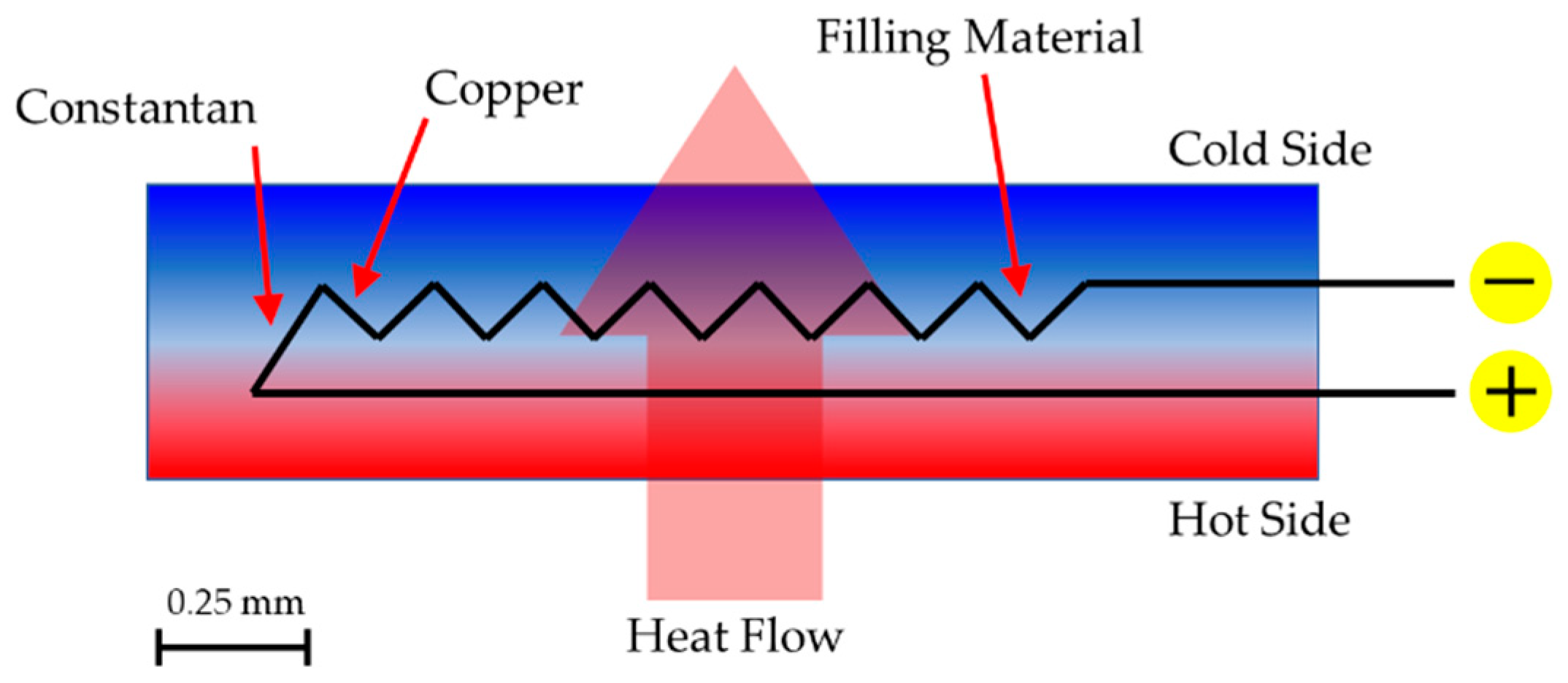
The heat flow sensor is a device that produces an electrical signal, and that signal is a linear function of the heat passing through the sensor. The sensors are usually flat, thermally resistive plates with thermocouples that have several thermophiles integrated into the thermocouple substrate (
Figure 1).
Temperature sensors are devices that produce an electrical signal, which is a linear function of its temperature. Minimally, two sensors must be used for the measurement of the U-value, one for the indoor and one for the outdoor air temperature.
Sensors (heat flowmeter and thermocouples) are mounted in such a way that ensures the result is a representative of the whole element. The best location for the mounting of the sensors can be determined by IRT, according to EN 13187 [
16]. Therefore, before the measurement, it is necessary to fulfil specific requirements according to ISO 9869 [
7]:
- (1)
Heat flux sensor should not be installed close to the parts with high thermal conductivity (i.e., thermal bridges), cracks, or other causes of error.
- (2)
The surface under examination has to be shielded from rain, snow, and solar radiation.
- (3)
Data acquisition intervals should be less than 30 minutes. This interval depends on the thermal inertia of the element, indoor an and outdoor air temperature difference, and method used for data analysis (AVGM or DYNM).
- (4)
The minimal measurement period should be 72 hours for stable boundary temperatures; otherwise, it should be more than seven days.
- (5)
The minimal indoor and outdoor air temperature difference should be 10 °C.
- (6)
It is necessary to achieve quasi-stationary conditions three to four hours before the measurement.
- (7)
The U-value should be approximated for the first 24 hours and 2/3 of the overall measurement period. These values should not vary more than 5% from the U-value calculated at the end of the measurement period.
2.1.1. Determining the U-Value According to ISO 9869
The HFM is a nondestructive method standardized in ISO 9869, and it is based on measuring the heat flow rate using a heat flow sensor while simultaneously measuring indoor and outdoor air temperatures using thermocouples. ISO 9869 gives two methods for analyzing measured data: the AVGM and the DYNM.
Average Method (AVGM)
The AVGM divides the average heat flow rate by the average temperature difference between the indoor and outdoor air. If the measurement period is long enough, then the approximated U-value is calculated using Equation (2) [
7]:
where q
j is the heat flux, T
i and T
e are the indoor and outdoor air temperatures, respectively, while index j counts the individual measurement.
For the IRT, the U-value is determined by Equation (3):
where q
rad and q
conv are approximated by the measured surface, reflected, and air temperatures as described in
Section 3.
Dynamic Method (DYNM)
The DYNM is regarded as a more advanced method [
7]. This method represents the heat equation with a set of parameters and the selected number of time constants (usually less than three). These parameters are adjusted using some curve fitting method to have the best possible fit to the measured data. The DYNM can be used even when significant changes in the measured values (heat flow rates and temperatures) are present. In the approximated heat equation, the element is modelled by its thermal conductance and a few time constants τ [
4].
Not many researchers used the DYNM described in ISO 9869 [
7] for calculating the U-value of building elements because of its complexity over the AVGM, as is stated by Ficco et al. [
17]. The complexity of the DYNM is also described by Mandilaras et al. [
18].
The DYNM assumes that the heat flux rate in some time j is a function of the temperature in that time step and all the previous time steps—Equation (4) [
7]:
where dynamic characteristics of the wall are K
1, K
2, P
n, and Q
n, and they have no real meaning. In Equation (4), p represents a subset of data points used for numerical integration corresponding to sum over j. The variables β
n are exponential functions of the time constant τ
n. Derivatives of indoor and outdoor air temperatures are calculated using Equations (5) and (6) [
7].
where Δt is the time interval between two measurements.
If m time constants are chosen (τ
1, τ
2, …, τ
m), then 2 × m + 3 unknown parameters are needed. These parameters are given by Equation (7) [
7]:
Equation (4) is written 2 × m + 3 times for 2 × m + 3 discrete time steps, and a system of equation is derived. By solving this system of equation, unknown parameters are determined. The first solution to that system of equations is the thermal transmittance or the U-value. One to three time constants are needed (τ
1 = r × τ
2 = r
2 × τ
3) to accurately represent the relation between the measured values (q, T
i and T
e) where r is the ratio between time constants [
7].
By using enough data sets at different time steps, an overdetermined system of equation is derived—Equation (8) [
7]:
where {q} is the vector with M elements that are the heat flow data measurements, [X] is a non-square matrix with M rows and 2 × m + 3 columns, and {Z} is the vector with 2 × m + 3 elements which are the unknowns. Since matrix [X] is not a quadratic matrix, it is not possible to find the inverse directly. In other words, Equation (8) represents a predefined linear system that can be solved by the classical least square method. The inverse of a non-square matrix can be determined by Moore–Penrose inverse [
19]—Equation (9):
where [X]
H is a complex conjugate transpose matrix and if its components are real numbers, which is true in this case, Equation (9) is then transformed into:
Substituting Equation (10) in Equation (8) approximated vector {Z}
* of the vector {Z} is calculated, and for every {Z}
* the approximated vector {q}
* is determined—Equation (11):
Equation (11) is solved by the least square method by varying the time constants τ
n through the procedure described in
Section 2.2.
2.2. Procedure for Determining the U-Value Using the DYNM
The DYNM given in [
7] is used for the analysis of data collected using the HFM. This paper aims to use the DYNM in combination with the IRT without the need for using a heat flux meter.
Even though the DYNM is more robust than the AVGM, it can be used for relatively fast and accurate in situ U-value determination.
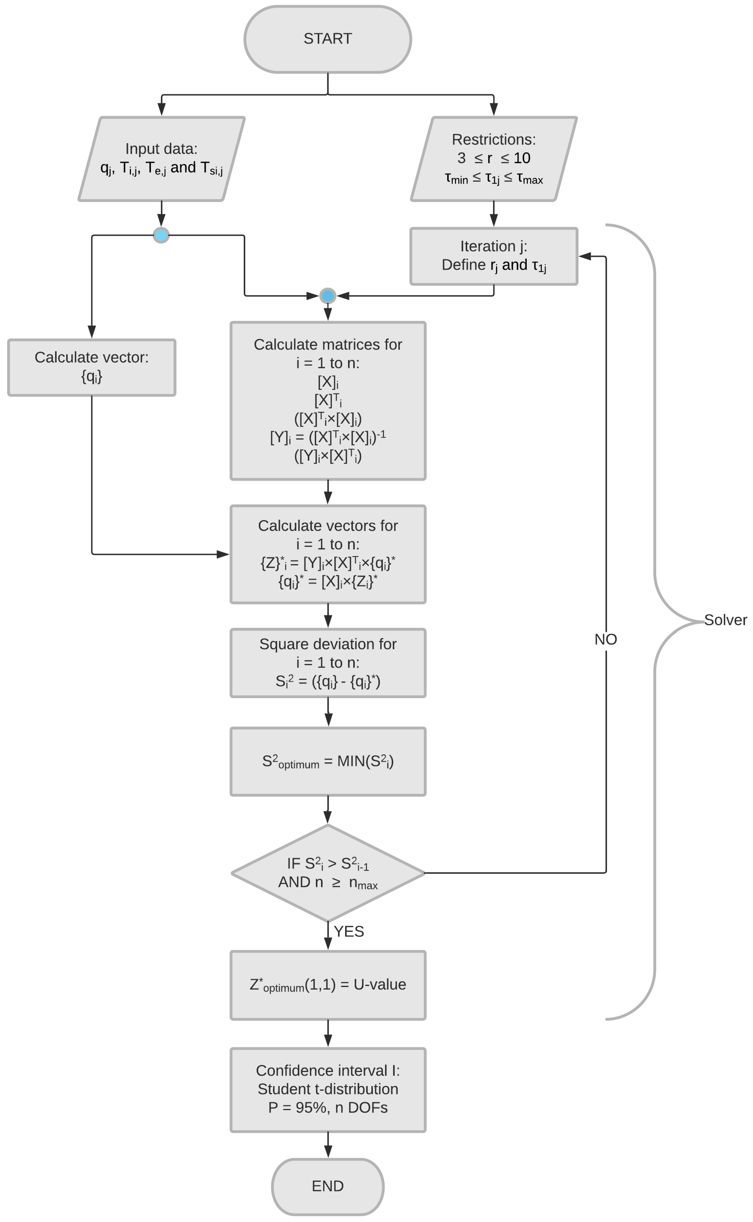
Figure 2 shows the flowchart programmed in Microsoft Excel VBA for implementation of the DYNM based on the least square approximation. The procedure described in ISO 9869 [
7] is as follows:
- (1)
Choosing m numbers of the time constants (1 ≤ m ≤ 3).
- (2)
Choosing the constant ratio between the time constants (3 ≤ r ≤ 10) in such way that τ1 = r × τ2 = r2 × τ3.
- (3)
Choosing the number of equations M (2 × m + 3 ≤ M ≤ N).
- (4)
Calculating the minimum and the maximum values of the time constants (Δt ≤ τ1≤ p × Δt/2).
- (5)
Calculating the estimated vector {Z}
* for the series of time constants using Equation (11),
- (6)
and estimate vector {q}* using Equation (12).
- (7)
Calculating the total square deviation between vectors {q} and {q}
* using Equation (13).
- (8)
Repeating the steps (5) and (6) until the smallest square deviation Smin is obtained.
- (9)
A good approximation {Z}* of the vector {Z} is obtained this way. The first component Z1 of vector {Z}* is the approximation of the U-value.
If the time constant τ1 is larger than the maximum value τmax = p × Δt/2, then the selected number of data points for the system of equations is not sufficient and results obtained in this way are not reliable (for a subset of data points M and ratio r).
The uncertainty is calculated using Equation (14) for the assessment of the results obtained using the selected data set [
7]:
where total square difference between {q} and its approximation {q}* is S
2, Y(1, 1) is the first element of the [Y] = ([X]
T × [X]
−1) matrix and F is a significance limit of Student’s t-distribution; where P = 0.95 is the probability and M −2 × m − 5 are the degrees of freedom.
If I is smaller than 5% of the U-value than the approximated U-value is generally very close to the actual value.
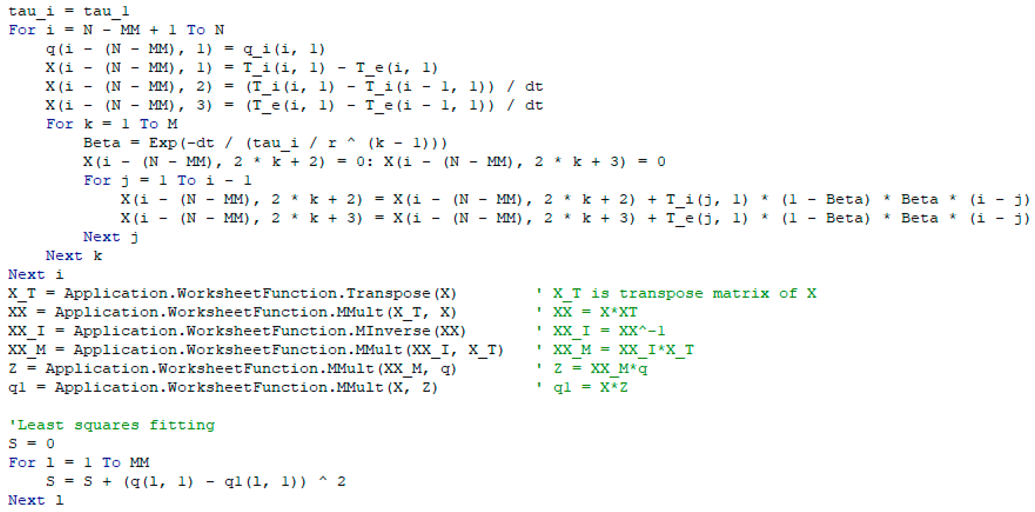
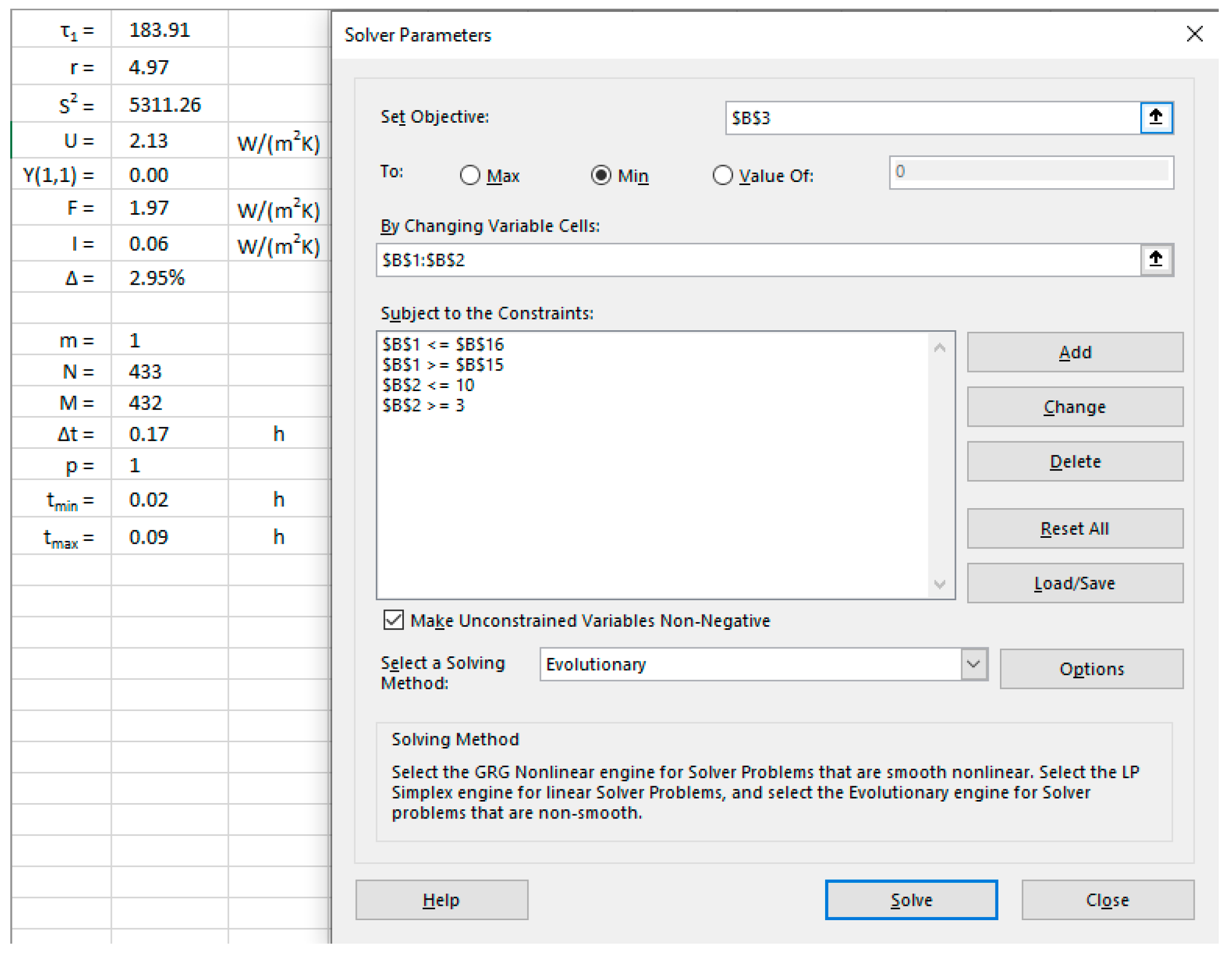
Excel add-in Solver was used for implementing the least square adjustment procedure.
Figure 3 shows a part of the code that makes the least square adjustment for time step j, and
Figure 4 shows Solver parameters used for the analysis.
2.3. Infrared Thermography (IRT)
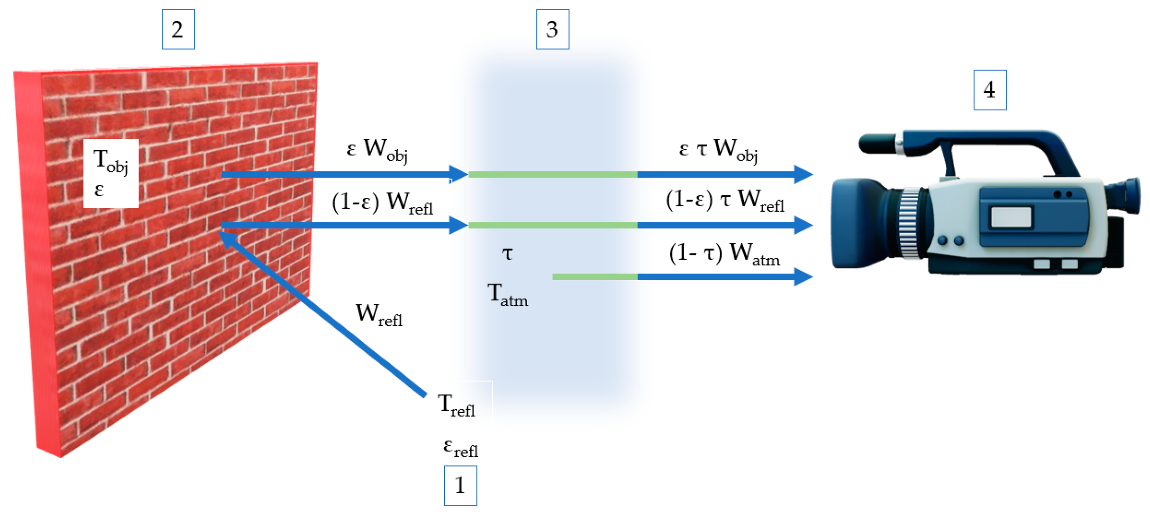
Figure 5 is showing the heat transfer scheme of an IRT analysis. Equation (15) is the energy balance during this process [
20]:
where W
tot (J) is total energy that reaches the camera lens when the surface is focused and W
obj (J) is radiated energy from the surface, and it is the only term of importance for measuring the surface temperature. The total reflected energy that reaches the examined surface is W
refl (J). It is a function of the average temperature of all the objects surrounding the surface under analysis, and the physical properties of the surface itself (mostly its reflectiveness). W
atm (J) is the total energy emitted by the atmosphere. It is the function of the air temperature, relative humidity (RH) and the distance between the IR camera and the examined surface. ε is surface emissivity, τ is the atmosphere’s transmittance, and σ is Stefan–Boltzmann constant [
20,
21].
Surface emissivity is mostly influenced by surface temperature, the wavelength of infrared radiation, and the angle at which the IR camera sees the surface. The angle at which the camera sees the surface is important due to the “Narcissus effect”—the camera is self-reflecting [
22]. For solid objects and relatively low temperatures (i.e., −10 °C to 50 °C), the change of the surface emissivity and wavelength with temperature can be ignored in most cases [
23]. Therefore, a single value of emissivity is typically assigned to the surface.
Furthermore, surfaces with a high level of emissivity release a higher amount of infrared radiation, and because of that, those surfaces reflect a lower percentage of radiation from the environment. Due to their low reflectivity, these surfaces are perfect for reliable determination of surface temperature using the IRT. If surfaces have a low level of emissivity, then they reflect a higher amount of radiation from the surfaces in their surroundings that have high temperatures (e.g., light bulbs, radiators, and people). Transparent surfaces (e.g., windows) behave like reflectors of infrared radiation, which makes it much more difficult to measure their surface temperatures using the IRT. Glass surfaces are the main problem when measuring the reflected temperature due to their high exposure to direct sunlight.
Therefore, for measuring the surface temperature using the IR camera, one needs to know the input parameters: surface emissivity, reflected temperature, indoor or outdoor air temperature, RH of the air, and distance between the surface and the IR camera.
3. The Surface Heat Transfer Coefficient
Since infrared thermography gives surface temperature distribution of the whole area that the camera sees, it is possible to approximate the total heat flux rate that passes through the building element rather than having discrete points where heat flux is measured (i.e., in the HFM). On the other hand, the main problem of the IRT lies in the determination of the surface heat transfer coefficients (both convective and radiative) since they are a function of several variables: free fluid flow speed, characteristic length, fluid thermo-physical properties, etc. Since heat transfer through the walls by conduction, in steady state conditions, equals the sum of the heat transfer by radiation and convection, it is possible to determine the heat flux that causes a transfer of heat from the fluid to the surface and vice versa—Equation (16):
where q
cond, q
conv, and q
rad are the heat transfer rates by conduction, convection and radiation (W/m
2), h
c and h
r are the convective and radiative heat transfer coefficients (W/(m
2 K)), T
i is the indoor air temperature, and T
si is the surface temperature (K).
For relatively low temperatures, like those in building physics (i.e., −10 °C to 50 °C), the radiative heat transfer coefficient basically has a constant value, like it is shown by Acikgoz [
24]. It is calculated using Equation (17).
where ε is the surface emissivity, and σ is Stefan–Boltzmann constant. h
r can also be calculated using the reflected surface temperature T
ref instead of T
si.
The convective heat transfer coefficient is highly influenced by airspeed and surface morphology. Three mechanisms of convective heat transfer exist: natural, forced, and mixed convection. Natural convection is described by the heat transfer inside the fluid in which the motion of the fluid is not caused by an outside force (e.g., by a pump or a fan) but only by the pressure variations inside the fluid (i.e., temperature gradients) [
25]. Forced convection is described by the heat transfer in which an external force generates the motion of the fluid (e.g., by a pump or a fan), and in mixed convection, both mechanisms are present—the temperature difference and the forced fluid flow [
25]. The theoretical formulae originated from the boundary layer theory of a vertical heated or unheated plate in an undisturbed surrounding. The theoretical local convective heat transfer coefficient is calculated by Equation (18) [
26].
where Nu and λ
f (W/(m K)) are the Nusselt number and thermal conductivity of the fluid (air in this case), respectively, and x is the distance (m) from the edge of the object that first contacts the air (i.e., leading edge).
Several factors influence the convective heat transfer coefficient. Such factors are surface geometry, surface surroundings, the position of the surface on the building, surface roughness, speed of air over the surface, local airflow whirls, and the surface to air temperature gradient [
16,
27,
28,
29]. There are different values for determining the convective heat transfer coefficient—analytical (theoretical), numerical, and experimental methods. Theoretical methods typically give minimum values of the convective coefficient. Numerical methods, primarily computational fluid dynamics (CFD), are a powerful tool for calculating both the internal and the external convective coefficients. However, CFD simulations, even with today’s technological advancements, require a substantial computational means. Experimental methods, both small-scale and large-scale, are still the main source for calculating the surface heat transfer coefficients. Empirical formulae are obtained from an extensive range of situations, and the temperature is usually measured in the center of the test chamber or at a location close to the wall. Surface heat transfer coefficient is determined from experimental data by the least square curve fitting using Equation (19). For natural convection, coefficient h
c can be expressed using Equation (19) for all surfaces [
5].
where C and n are constants that are used for the curve fitting, and ΔT = T
i − T
si.
Table 1 shows various choices for constants C and n for the natural convection with the name of the authors who calculated the empirical expressions. The formula for h
c in
Table 1 is derived from experimental data sets using Equation (19).
If the flow is laminar, then empirical formulae used for calculating the convective heat transfer coefficient can also be taken from Bejan [
38] and Chu [
39]—Equation (20):
where H is the wall height (m) or surface height if the wall is composed of more than one surfaces.
The formula that can be used for both the laminar and the turbulent flow is suggested by Almadari and Hammond [
40]—Equation (21):
Wallenten et al. [
41] derived their formula from full-scale experiments. The formula gives somewhat greater value than analytical or small-scale experiments.
Another approximation for the convective heat transfer coefficient is given in ISO 9869 [
7] as usually assumed value of 3.00 W/(m
2K) for vertical surfaces that are not directly heated or near windows where the surface is not plain.
Procedure for Calculating the Convection Heat Transfer Coefficient of Vertical Isothermal Planes
The theoretical convection coefficient is calculated by Equation (18). Before hc can be calculated, Nusellt, Grashof, and Rayleigh numbers are needed. The analytical procedure for calculating the average convective heat transfer coefficient is described below.
All thermal properties are calculated for the film temperature T
f—Equation (22) [
42]:
Grashof number is calculated using Equation (23) [
25]:
where g is gravitational acceleration (m/s
2), L is the height of the vertical surface (m), ν is cinematic viscosity (m
2/s), and β represents the temperature coefficient of thermal conductivity (K
−1). β is equal to the 1/T
f.
Equation (24) gives the Rayleigh number [
25]:
where Pr represents the Prandtl number of the convective fluid at T
f. The average Nusselt number is given by Churchill and Chu [
39]—Equation (25):
Equation (26) gives the average local convection coefficient for the whole area for a vertical isothermal plane [
25]:
5. Results
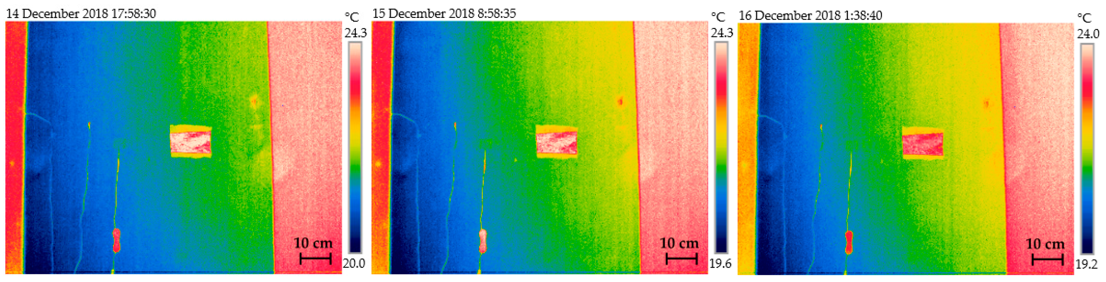
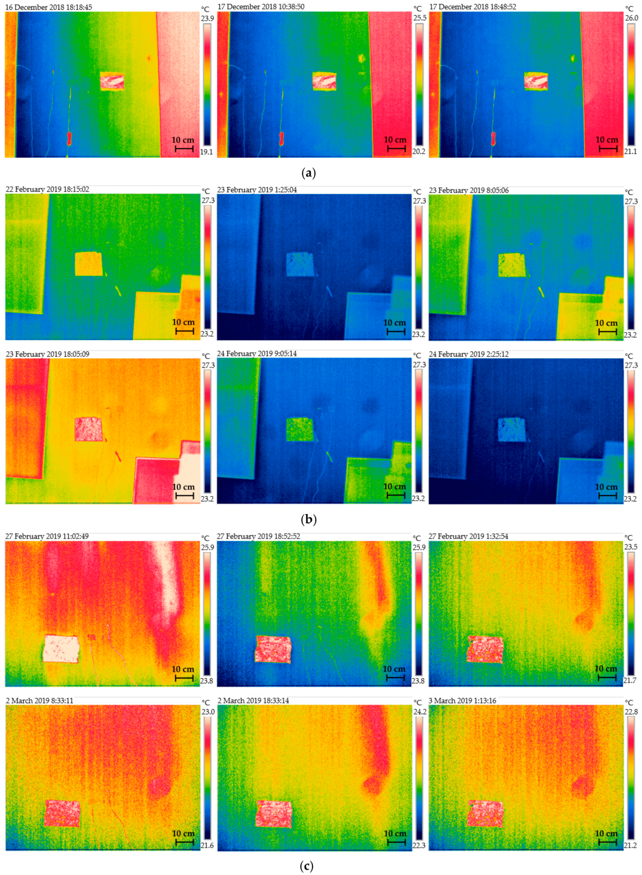
Figure 9 shows input data for approximating the U-value using the IRT and the HFM.
Using the collected datasets from all three measurements, the U-values and uncertainties using the AVGM (Uavg) and the DYNM (Udyn) were determined. One time constant was adopted because it gave the best confidence interval (from 2.13 to 3.87%). For two and three time constants, τ it was not possible to get satisfactory confidence interval I, and because of the large number of data points, for three time constants analysis time was around 30 minutes.
To minimize the measurement period, the same sets of data were used for the approximation of the U-value after one, two, and three days. The U-value calculated after one and two days was then compared to the U-value calculated after the three-day measurement period.
The first thing that can be noticed in
Figure 9 is that for all three walls, the approximated function of the heat flux is similar to the function acquired by the HFM. For Wall 1, the approximated function is translated from the measured heat flux function due to the significant impact of air blowing through the window gaps, which is seen in
Figure 9a. The heat convection over the surface of Wall 1 is not natural, but it is forced by air blowing through the gaps. Secondly,
Figure 9 also shows the convergence of the U-value for the AVGM. That convergence is similar for both the IRT and the HFM.
Table 6 shows a comparison of the U-values determined using the HFM and the IRT, together with the variation of the measured U-values depending on the convective heat transfer coefficients given by different authors. These tables show that one needs to be careful in choosing which convective heat transfer coefficient is being used.
Table 7 shows the minimal and maximal values of the approximated U-values for different convection coefficients. From
Table 7, it can be seen that the convection coefficient affects the U-value significantly and that difference was 5%–32% depending on the duration of the measurement, formulae used for the convection coefficient approximation, and the method used for the measurement and the analysis.
For Wall 1, the U-value approximated using the IRT is closer to the designed value—the maximum error was around 19% if the measurement period was equal to three days and if the theoretical convective heat transfer coefficient was used. On the other hand, if Wilkers et al. [
36] empirical formula was used for determining the convective heat transfer coefficient, then the difference between the design and the dynamic U-value was only 0.11%.
Furthermore, if the measurement period was one or two days, the DYNM gave similar results compared to the results acquired for three days measurement period. The best values are acquired for Nusselt [
34] empirical formula for the convective heat transfer coefficient (
Table 1). The difference was 0.41%–5.37% irrespective of the method used for calculating the convective heat transfer coefficient. The U-value approximated using the HFM differed from the designed value by 22% to 30% if the measurement period was equal to three days (for both the AVGM and the DYNM). It can be observed in
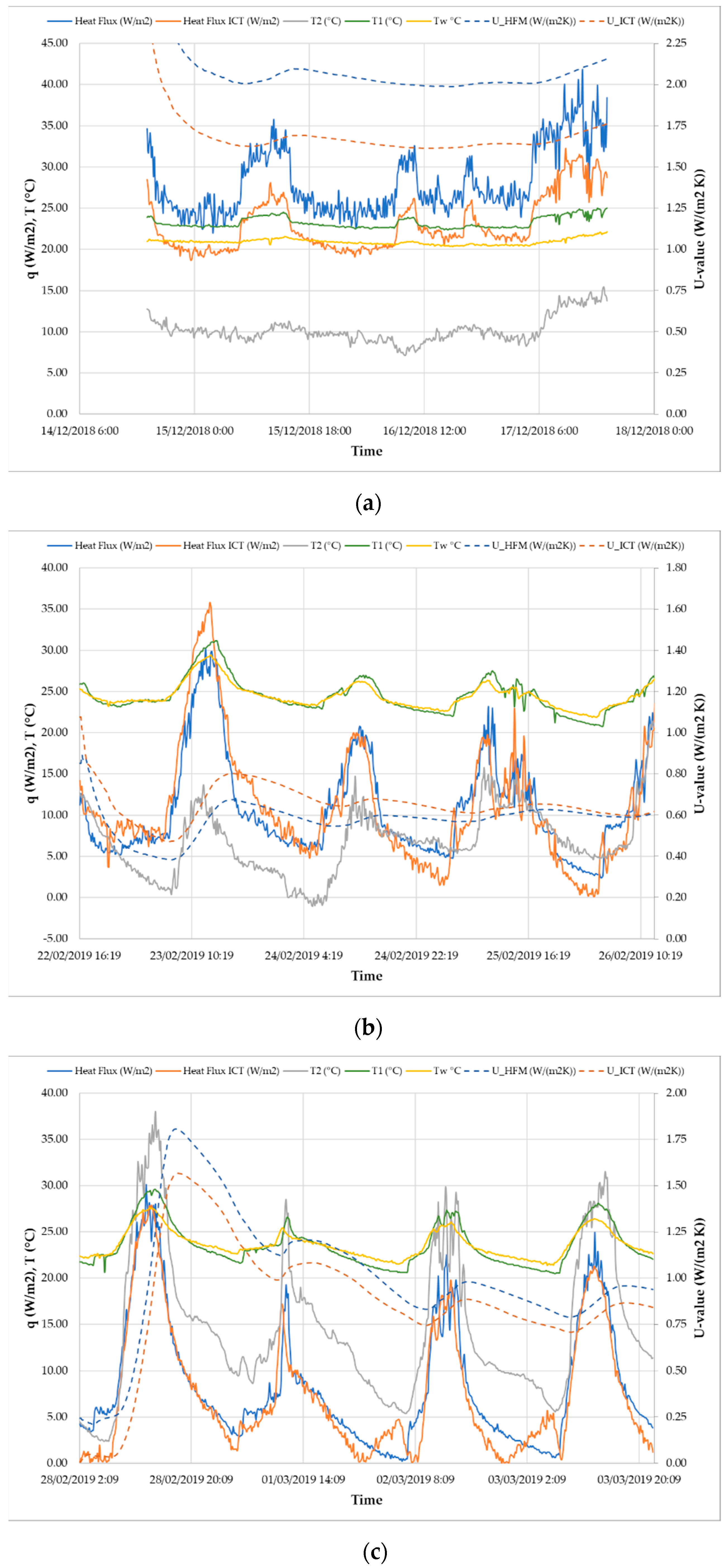
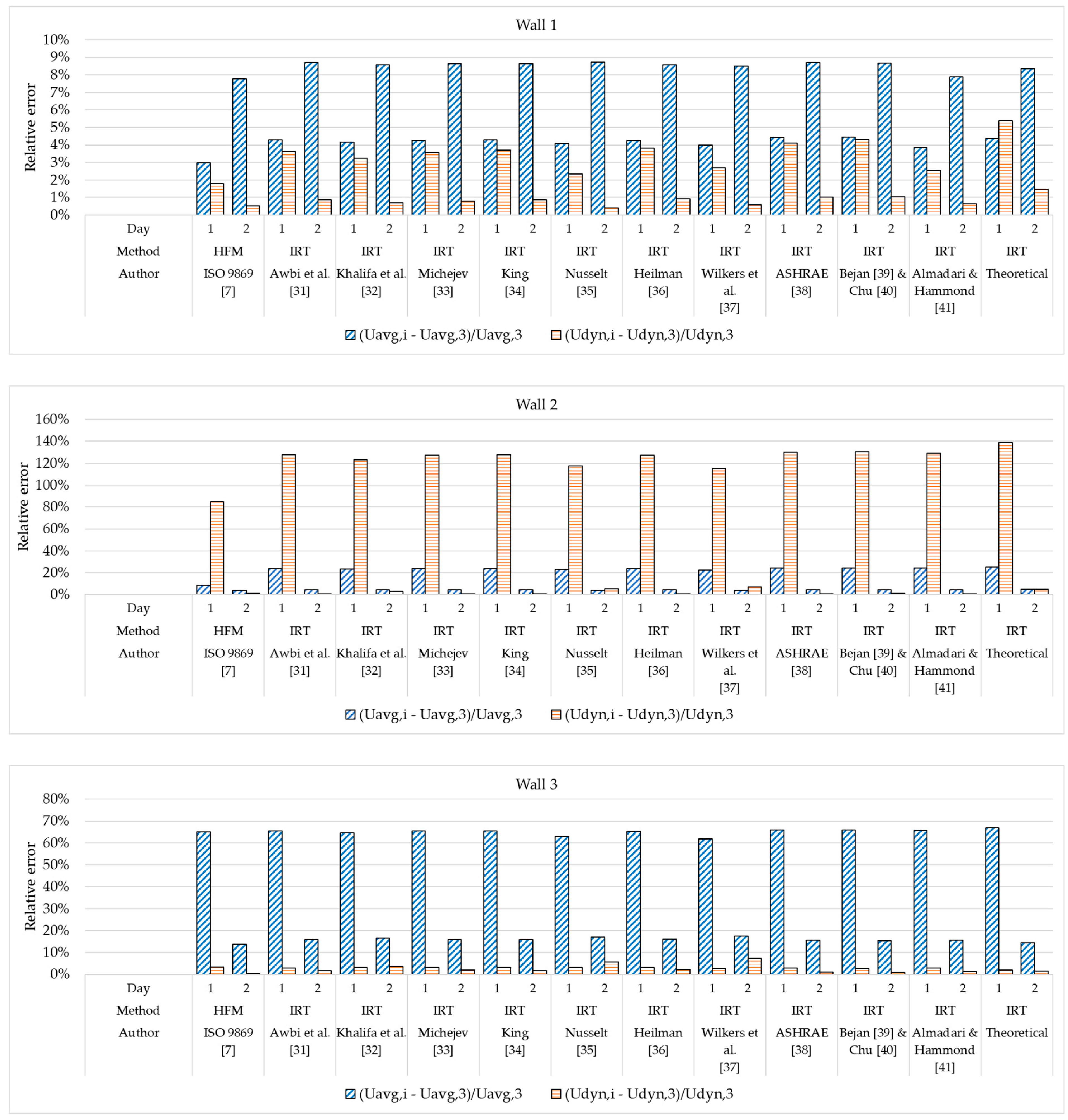
Figure 10 that the DYNM was more stable than the AVGM for any measurement period—the difference between the U-value calculated after one and two days was less than 2% of the U-value approximated after three days. If the AVGM was used, the maximal difference was around 7%.
For Wall 2 and Wall 3, both the DYNM and the AVGM gave similar absolute differences between the U-value approximated using the IRT and the designed U-values. For Wall 2, the DYNM gave a 30% higher U-value compared to the designed value, while the AVGM gave 30% smaller U-values. Results were similar with Wall 3, where the difference is ±20%. The approximated U-values for both the IRT and the HFM are shown in
Table 6. If Wilkers et al. [
36] empirical formula was used for the determination of the convective heat transfer coefficient, then the difference between the designed and dynamic U-value was 26.01% for Wall 2 and only 1.95% for Wall 3.
If the measurement period was one or two days, the DYNM gave similar results compared to those acquired for three days measurement period for Wall 3, where that difference was approximately 0.34%–7.19% (
Figure 10). For Wall 2 that was true for two-days measurement period where the difference was approximately 0.16%–7.19% (
Figure 10), and for one day measurement period the difference was 120% (
Figure 10) which might have been caused by direct solar radiation on the thermocouples and indirect radiation reflected from the windows that were overheated by sunlight. The effect of solar radiation is seen in
Figure 9b,c.
The difference between the U-values calculated using the AVGM and the DYNM differs significantly. That difference was approximately 80% for Wall 2 and 25%–50% for Wall 3. Since boundary conditions were not stable during the measurement period (
Figure 9b,c), it can be concluded that results obtained by the AVGM are not satisfactory which can also be seen from the standard deviation of the AVGM shown in
Table 6. It can also be observed, just like in the case of Wall 1, that the DYNM was more stable than the AVGM.
The difference between the U-values approximated using the IRT and calculated from the HFM measurements was approximately 4.25%–7.81% for Wall 2 for the AVGM after the measurement period of three days, and 0.80%–3.81% for the DYNM for the same measurement period. For Wall 3, that difference was more significant—12.33%–16.48% for the AVGM and 0.11%–21.76% for the DYNM.
The difference between the U-value approximated after the three-day measurement period, between Wall 2 and Wall 3, which have the same composition, varied from 28.43% to 46.02% for the IRT and the AVGM of analysis, and for the DYNM, the difference varied from 1.99% to 23.60%. For the HFM, the difference is approximately 17.21% for the AVGM and 1.68% for the DYNM.
6. Conclusions and Further Research
This paper shows that there is potential for using the IRT for calculating the U-value in real environmental conditions in-situ.
The surface examined in this paper is not isothermal, and the paper shows that by using the IRT it is possible to approximate the U-value with a high level of accuracy compared to traditional methods (i.e., HFM). The differences between the U-values approximated using the IRT, and the designed U-values are between 0%–19% for Wall 1, ±30% for Wall 2, and ±20% for Wall 3, irrespective of the method used to calculate the convective heat transfer coefficient.
It is shown that for all three Walls, the approximated function of the heat flux acquired by the IRT is similar to the function acquired by the HFM, thus confirming the feasibility of using the IRT. For Wall 1, the approximated function is translated from the measured heat flux function because of the significant impact of air blowing through the window gaps. The heat convection over the surface of Wall 1 is not natural, but it is forced by air blowing through the gaps.
Furthermore, it was shown that the DYNM, in combination with the IRT, could be used for relatively faster and accurate in-situ U-value approximation. This paper shows the potential for the reduction of the time needed for the measurement without losing the accuracy of the results. It is shown that with the use of the IRT and the dynamic analysis method, the duration of the measurement could be reduced by 30%, or even by 60%, compared to the length of the measurement when using the HFM and the AVGM. The IRT also has the advantage of detecting the surface heat changes during time, which can be useful for minimizing the thermal bridging effects and detecting air movement over the surfaces.
The differences between the U-values approximated using the IRT and the HFM are approximately 4.25%–16.48% for the AVGM, and 0.11%–21.76% for the DYNM.
Furthermore, if the measurement period is reduced, then the differences between the U-values calculated after one or two days, for Wall 1 and Wall 3, are around 5%–20% of the U-value calculated after three days and if the AVGM is used. If the DYNM is used, then that difference is approximately 0.34%–7.19%. For Wall 2, that difference is highly affected by overheating due to the sunlight. Thermocouples are overheated by both direct solar radiation and indirect radiation reflected from the windows. If the measurement period is reduced, then the differences between the U-values calculated after one or two days are approximately 15%–70% for the AVGM and 0.16%–120% for the DYNM.
Determination of the U-value by infrared thermography is still under development. To improve the given model, both the HFM and the IRT should be simultaneously used so the surface heat transfer coefficients can be determined and correlated for future references. These measurements will give further insight into why these differences occur and which method is better and under which conditions.


