Deep-Learning-Based Automated Building Information Modeling Reconstruction Using Orthophotos with Digital Surface Models

Abstract

In the field of building information modeling (BIM), converting existing buildings into BIM by using orthophotos with digital surface models (DSMs) is a critical technical challenge. Currently, the BIM reconstruction process is hampered by the inadequate accuracy of building boundary extraction when carried out using existing technology, leading to insufficient correctness in the final BIM reconstruction. To address this issue, this study proposes a novel deep-learning- and postprocessing-based approach to automating reconstruction in BIM by using orthophotos with DSMs. This approach aims to improve the efficiency and correctness of the reconstruction of existing buildings in BIM. The experimental results in the publicly available Tianjin and Urban 3D reconstruction datasets showed that this method was able to extract accurate and regularized building boundaries, and the correctness of the reconstructed BIM was 85.61% and 82.93%, respectively. This study improved the technique of extracting regularized building boundaries from orthophotos and DSMs and achieved significant results in enhancing the correctness of BIM reconstruction. These improvements are helpful for the reconstruction of existing buildings in BIM, and this study provides a solid foundation for future improvements to the algorithm.

1. Introduction

With the acceleration of urbanization and the development of BIM technology, it has become increasingly important to efficiently and accurately acquire building information models (BIMs) for existing buildings. As a digital building model that integrates a large amount of information, BIM supports the entire life cycle management of buildings using digital technology. In addition to simple geometric information, the building components contained in BIM also include the building’s engineering information. This ensures that BIM covers every aspect of the building, from design to construction to operation and maintenance. However, many existing buildings do not have corresponding digital models that were developed during design and construction due to their age and thus cannot be integrated into modern construction management systems. Therefore, it is necessary to collect and analyze the data for existing buildings and then reconstruct BIMs to realize the digitization of existing buildings.

During BIM reconstruction of existing buildings, there were several problems that were encountered when using traditional methods. Manual mapping or reconstruction based on point clouds obtained from 3D laser scanning [1] can accurately restore building data but are often time-consuming and costly, especially when performing large-scale BIM reconstruction [2]. In recent years, with the continuous advancement of high-precision drone and satellite technologies, the technique of BIM reconstruction with the help of easy-to-acquire orthophotos and DSMs has emerged not only because it can significantly reduce the time and cost of data acquisition [3], but also because it meets the urgent demand for large-scale BIM reconstruction of existing buildings [4]. Orthophotos provide distortion-free top-view images of buildings [5], which are essential for accurately determining building boundaries. Meanwhile, a DSM provides elevation information on a building and its surroundings, which can be used to determine the building’s height. Combining these two data sources enables the automated BIM reconstruction of buildings. This process eliminates the need for costly ground surveys or direct physical contact, significantly improving the efficiency of data collection and reducing acquisition costs [6].

The greatest challenge in automatic BIM reconstruction using orthophotos and DSMs is the need to extract accurate and regularized building boundaries from the orthophotos and DSMs. Although previous research [7,8] employed deep-learning and image-processing methods to achieve regularized building boundary extraction, most of these studies rely on either orthophotos or DSMs as a single data source. The surface texture and color information of buildings as determined from orthophotos, as well as the surface elevation changes provided by DSMs, are valuable data. However, to extract accurate and regular building boundaries from two data sources, a feature extraction method that can integrate different data types is needed.

Moreover, in past building reconstruction research, the city geography markup language (CityGML) standard was commonly used to construct three-dimensional building models [9,10,11]. The three-dimensional models reconstructed based on the CityGML standard contained geometric information about building components. However, these models were relatively limited in their cover of the building’s intrinsic engineering properties and performance information and could not expand upon or supplement subsequent information, leading to limitations of CityGML in engineering applications. As a new and constantly developing digital technology, BIMs are more widely used in the design, construction and operation, and maintenance management stages of actual construction projects because of their more advanced information organization and interactivity [12]. Nonetheless, because the automated interaction between BIMs and external data is more complex, there are relatively few studies that cover automatically reconstructing BIM using orthophotos and DSMs.

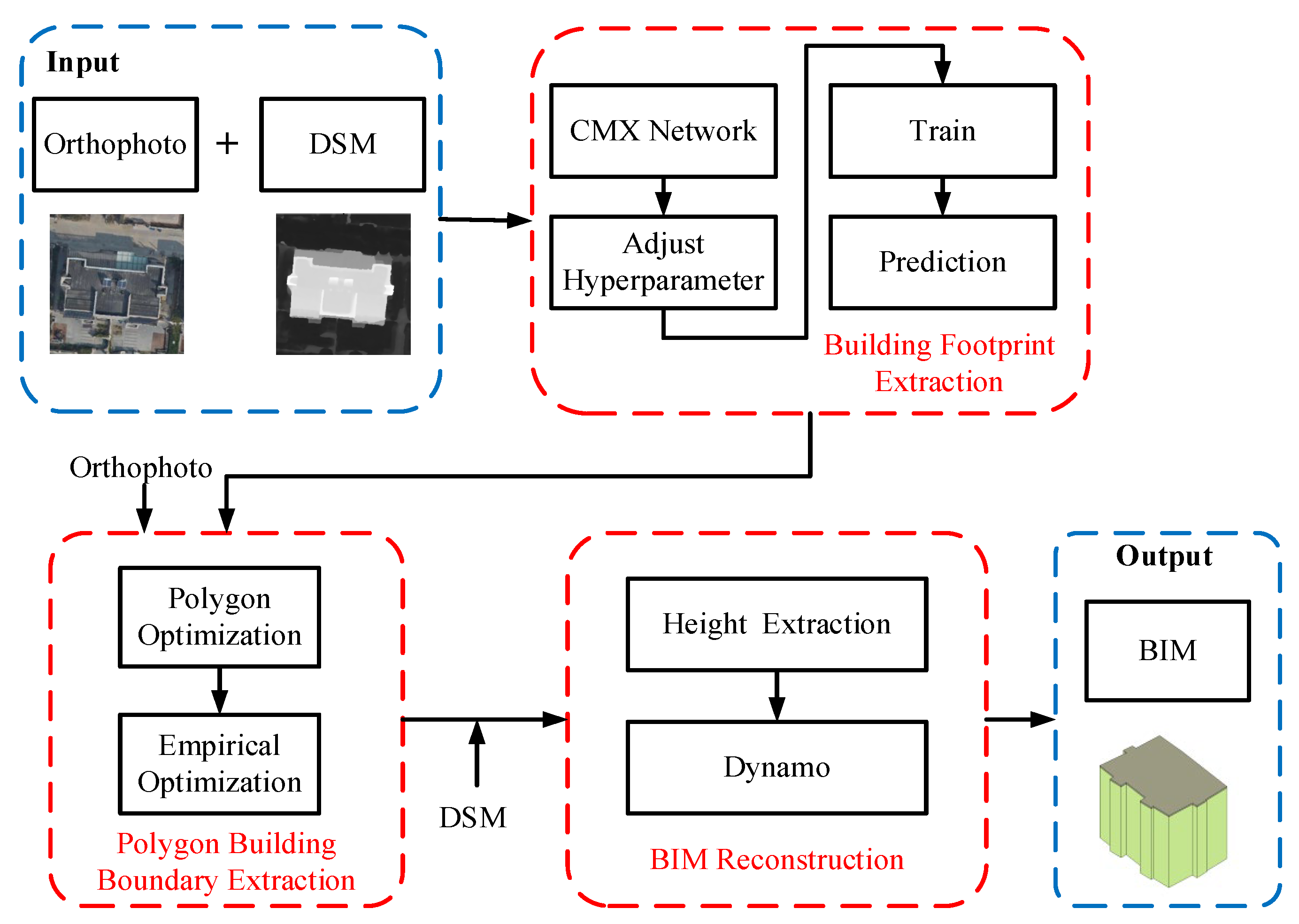
In view of these challenges, this study proposes a new method of automatically reconstructing BIM from orthophotos and DSM data. First, a deep-learning network that fuses orthophotos and DSM data are fused to more accurately accomplish building footprint extraction. Then, polygon optimization with empirical optimization is used to accurately extract polygonal building boundaries. Finally, the elevation information in DSMs is utilized to obtain the building height, and the building boundary and height information is used by Dynamo to reconstruct the BIM in Autodesk Revit.

2. Literature Review

Three-dimensional building reconstruction techniques based on orthophotos and DSMs have attracted extensive academic attention. Partovi et al. [13] used methods combining DSMs with multispectral satellite orthophotos to achieve the extraction, decomposition, and connection of building boundaries, culminating in the reconstruction of three-dimensional building models. Mao et al. [14] employed deep-learning techniques to predict potential DSMs from orthophotos, aiming to reconstruct three-dimensional building models using the input orthophotos. Gui et al. [8] adopted a model-driven strategy to extract features from DSMs and ultra-high-resolution satellite orthophotos for the reconstruction of building models. Yu et al. [15] replaced the traditional multi-view stereo vision (MVS) methods with deep-learning strategies, transforming multi-angle drone images into DSMs and orthophotos for the purposes of three-dimensional building reconstruction. These studies generate building models that conform to the CityGML standard and are widely applied in the field of Geographic Information Systems (GISs), but there is considerably less research on BIM reconstruction.

Mainstream building reconstruction studies have usually incorporated a data-driven framework with three key steps: semantic segmentation of buildings, boundary extraction, and 3D model reconstruction. In the semantic segmentation phase, deep-learning methods, especially classical convolutional neural networks (CNNs) [16,17,18] and the latest Transformer architecture [19] have become the preferred techniques due to their excellent classification performance in complex contexts. These techniques are able to improve the accuracy of building extraction compared to that of traditional imaging methods. At the same time, multi-modal semantic segmentation technology that integrates deep orthophotos and DSMs continues to emerge. SA-gate [20] introduced a unified and efficient cross-modal guided encoder to improve the performance of RGB-D semantic segmentation. Zhou et al. [21] developed an end-to-end feature extraction and gate fusion network, CEGFNet, to achieve high-precision semantic segmentation from DSMs and orthophotos.

Subsequently, semantically segmented images of buildings are usually postprocessed during a boundary extraction session. The simplest approach is to apply the Marching Cubes algorithm [22] and Douglas–Peucker algorithm [23] to simplify the building boundaries or to use algorithms to regularize them. There have been studies dedicated to combining the semantic segmentation of buildings with the regularized extraction of contours with the aim of simplifying the process through an end-to-end deep-learning approach. By learning to build a segmentation map that is aligned with the proposed frame field vectors, Frame-Field [24] obtains building polygons through corner-aware contour simplification. Zorzi et al. [25] proposed polyworld, which uses CNNs to detect building boundary vertices and employs graph neural networks to predict the connection strength between vertices, ultimately realizing regularized boundary extraction by solving a differentiable optimal transport problem. Xu et al. [26] used a hierarchical supervision mechanism to complete polygonal building extraction using deep learning. Although these approaches show potential for automation, they rely on large-scale datasets with long training times. This has led to studies suggesting that combining deep learning with postprocessing may be more practical [27]. However, there are few studies on how to fully utilize the features of orthophoto and DSM data and apply both data types to the two phases of deep learning and postprocessing.

3. Methodology

Figure 1 shows the overall flow of the automatic BIM reconstruction method proposed in this study. The method takes orthophotos and DSMs as inputs and outputs a BIM with a level of detail (LOD) of 100. This study follows the classical data-driven approach, and the whole reconstruction process is divided into the following three steps:

• Building footprint extraction: combining orthophoto and DSM data, the latest multimodal semantic segmentation network technology is used to realize the high-precision semantic segmentation of the building area.
• Building boundary extraction: with the help of a polygon optimization algorithm and empirical rules for postprocessing the image to be semantically segmented, the polygonal boundaries that conform to the actual building shape are extracted.
• BIM reconstruction: the height of each building is determined by analyzing the DSM data and using the Dynamo 2.1 visual programming tool to automatically generate a BIM in Autodesk Revit 2020 software in batches.

3.1. Building Footprint Extraction

This study adopted the CMX (Cross-Modal Fusion for RGB-X) semantic segmentation network [28] for building footprint extraction; this is a cross-modal fusion framework based on ViT (Vison-Transformer) [29] for the semantic segmentation of RGB-X data sources, where X stands for a modality that is complementary to RGB. Through cross-modal fusion, the CMX network can improve the accuracy of semantic segmentation. Experimental results obtained using multiple sources of benchmark data proved that the CMX network is able to effectively fuse multi-modal data [28]. Without consuming a large amount of computing resources, the semantic segmentation accuracy reaches state-of-the-art levels. Since the postprocessing operation carried out in this article relies on semantic segmentation accuracy, the CMX semantic segmentation network was selected.

Figure 2 demonstrates the structure of the CMX network, which takes orthophotos as the input of RGB data and DSM data as the complementary-modality input and employs two parallel backbone networks to separately process the two types of data. CMX uses the classical encoder–decoder architecture. In the encoder stage, the features of the two modalities are extracted separately by using the efficient feature extraction module in Segformer [30], and the features of the current modality are corrected by using a cross-modal feature correction module (CM-FRM). Finally, the features of both modalities are globally enhanced by using a feature fusion module (FFM). In the decoder stage, the DeeplabV3+ [31] decoder combines the low-level features generated by the FFM with high-level ground detail information to further enhance the semantic segmentation accuracy.

3.2. Extraction of Polygonal Building Boundaries

3.2.1. Optimization Algorithm for Building Footprint Polygons

Semantic segmentation can be used to categorize each pixel and identify pixels belonging to building and non-building categories. However, although the DeeplabV3+ decoder used by the CMX network facilitates the recovery of details, the linear interpolation method used in its up-sampling process leads to insufficient accuracy of building edges in the semantic segmentation maps, especially when dealing with complex or zigzagging edges, which are significantly biased compared to actual regular building walls.

Postprocessing semantic segmentation results is a common measure to improve semantic segmentation accuracy. Superpixel optimization technology is an effective postprocessing method. Superpixel optimization technology optimizes semantic segmentation results by fusing the high-level semantic features of semantic segmentation and object edge information of superpixels. This postprocessing method does not greatly improve the overall accuracy, but it has a better optimization effect on semantic segmentation object boundaries. The goal of this article is to extract regularized building boundaries. Inspired by traditional superpixel optimization methods, this article hopes to use regular superpixels to optimize semantic segmentation boundaries. Therefore, this study adopted the polygonal partitioning technique [32] to optimize the results of semantic segmentation. Figure 3 shows the principle of the polygonal partitioning technique. For a given orthophoto, the technique first identifies straight line segments in the image by using an LSD (line segment detector) [33]; next, these detected line segments are extended in the image plane until they intersect with each other, thus segmenting the image into fine polygonal units. Finally, the smaller polygonal units are merged into larger polygonal units.

The polygonal partitioning technique draws on hyperpixel technology, which is based on the similarity of pixel positions and colors in an image and clusters the original pixels into hyperpixels. Hyperpixel methods such as simple linear iterative clustering (SLIC) [34] can effectively simplify the complexity of images. However, as shown in Figure 4, the hyperpixel blocks that they generate have an irregular morphology, which is unsuitable for building extraction scenes that require regular boundaries. Compared to the traditional hyperpixel technique, the polygonal segmentation technique focuses on generating regularized polygons that are more compatible with the structural features of buildings. This technique optimizes the regularity and smoothness of building boundaries in semantically segmented images and lays a solid foundation for subsequent boundary extraction steps.

The optimization of the building footprint is achieved by combining the high-level semantic features of semantic segmentation with edge information from the polygon optimization. Specifically, after obtaining the initial semantic segmentation results output by CMX, the orthophoto is then polygonally segmented, the number of pixels of different semantic categories within each polygon is counted, and the semantic category with the highest number of pixels is assigned to that polygon to achieve optimization. The specific algorithm is shown in Algorithm 1.

Algorithm 1: Polygon Optimization Algorithm
Input: Orthophoto O, Initial Semantic Segmentation Results I
Output: Optimized Semantic Segmentation results L
1	Define semantic categories C = {C_1, C_2} where C_1 = ‘building’ and C_2 = ‘non-building’
2	Partition orthophoto O into n polygons S = {S_1, S_2, …, S_n} using polygonal partitioning technique, where each polygon S_i contains m pixels p_j
3	Initialize L to be an empty image of the same dimensions as O
4	for each polygon S_i in S do
5	Initialize count N_1, N_2 to 0 for each category in C
6	for each pixel p_j in polygon S_i do
7	if p_j in I corresponds to ‘building’ then
8	Increment N_1 (count of ‘building’ pixels)
9	else if p_j in I corresponds to ‘non-building’ then
10	Increment N_2 (count of ‘non-building’ pixels)
11	end if
12	end for
13	if N_1 > N_2 then
14	Assign ‘building’ label to all pixels in polygon S_i in L
15	else
16	Assign ‘non-building’ label to all pixels in polygon S_i in L
17	end if
18	end for
19	return L

Figure 5 shows an example of the semantic segmentation results and a comparison before and after applying the polygon optimization algorithm. The left side shows the original unoptimized semantic segmentation results (green pixels denote buildings) superimposed on the orthophoto, where it can be observed that the semantic segmentation was less effective at the edges of the buildings. The right side shows the result after processing with the polygon optimization algorithm. The optimized semantic segmentation map has more regular and accurate building regions, especially in the building edge region. In the middle is a zoomed-in image of local details to provide a visual comparison. It is clear from this that the optimized semantic segmentation map matches the original image more closely at the edges of the objects, indicating that the high-level semantic information of the semantic segmentation was successfully fused with the edge information of the hyperpixels, thus improving the accuracy of the semantic segmentation. This comparison demonstrates that the polygon optimization algorithm improved the accuracy of semantic segmentation, especially when dealing with regular building edge details.

3.2.2. Empirical Optimization of Building Boundaries

To accommodate the input image size constraints imposed by deep-learning models, high-resolution orthophotos and DSMs need to be segmented into smaller plots. This cropping process may result in a single building spanning multiple plots, which, in turn, affects the continuity of the building footprint. In addition, there is an inherent edge effect in deep-learning models when dealing with the edge regions of the plots, which may trigger a prediction error in building boundaries when the plots are stitched together. To address the above issues, this study employed a sliding-window cropping strategy in the building footprint prediction stage, setting a 50% block overlap rate to ensure continuity. After obtaining the prediction results using semantic segmentation and polygon optimization, this study took the approach of removing 25% of each block boundary and using only the remaining center part for seamless stitching to construct the building footprint prediction map for the entire test area.

Next, the building footprints on the complete prediction map were initially extracted to recognize the connected building pixel blocks as independent building entities. The extraction of the initial building boundaries was accomplished using the Marching Cubes [22] and Douglas–Peucker algorithms [23]. This study further employed an empirical optimization approach to building contouring that applied a set of empirical rules to improve the accuracy of the extracted polygonal building boundaries. These rules were based on typical building characteristics, such as requirements for the minimum area and side length, and they limited the occurrence of overly sharpened or blunted angles [27]. An example of the application of these rules is shown in Figure 6. By repeatedly applying these rules, the obtained building contours were further refined to generate building boundaries that were closer to the actual situation.

3.3. BIM Reconstruction

3.3.1. Building Height Estimation

In order to complete the BIM reconstruction, in addition to obtaining the building boundaries, the height of the building within the boundary should also be obtained. The building height is the distance from the foundation to the roof of the building. The nDSM recorded the height information of the ground and all objects, and the building height was extracted from the nDSM. Figure 7 shows the relationships between the DSM, nDSM, and DEM, and the nDSM was obtained by subtracting the DSM from the DEM.

The formula of nDSM is as follows:

$$nDSM\left(i,j\right)=DSM\left(i,j\right)-DEM\left(i,j\right)$$

(1)

where

• $nDSM(i,j)$—the elevation value of nDSM in row $i$ and column $j$;
• $DSM(i,j)$—the elevation value of DSM in row $i$ and column $j$;
• $DEM(i,j)$—the elevation value of DEM in row $i$ and column $j$.

In this study, a cloth simulation filter (CSF) [35] method was used to estimate the DEM from the DSM, and the obtained DSM data were used to subtract the raster data from the DEM to obtain a digital model containing only the elevation information of the surface objects, i.e., the nDSM. After obtaining the nDSM, it was combined with the regularized contour maps of the buildings that were obtained, and the maximum value in the nDSM data was extracted as the height of the building within each building boundary.

3.3.2. Data Storage

The vertices of a building were identified by analyzing its polygonal contours and were represented as a series of coordinate points that defined its relative position in the orthophoto coordinate system. By multiplying these coordinates by the ground sample distance (GSD), they were converted into the relative positions of building boundaries in the real world. At the same time, building height information was extracted from the nDSM and recorded in an Excel workbook for subsequent use.

Table 1. An example of the storage of building boundaries and heights.

	A	B	C
1	X(m)	Y(m)	Height(m)
2	1712.3	714.4	14.11
3	1711.8	719.4	14.11
4	1710.5	722	14.11
5	1711.1	722.5	14.11

provides a typical example of the storage of the building vertex and height information. Each closed polygon represented a separate building, and its planar coordinates and height data were recorded in separate worksheets in an Excel workbook.

3.3.3. LOD100 BIM Reconstruction

The entire BIM reconstruction process was implemented in the Autodesk Revit 2020 software with the help of Dynamo 2.1, and a graphical interface was employed instead of the traditional text-based coding approach. Visual programming allows users to script and build logical structures by dragging and dropping graphical blocks, an approach that increases intuitiveness and simplifies the scripting process compared to text-based programming languages [36]. Figure 8 illustrates the core blocks in the BIM reconstruction methodology.

In this method, the vertex coordinates and height data of the building profile were imported from different worksheets of an Excel 2020 workbook by using Dynamo’s “Data.importExcel” module. The coordinates of the vertices (x,y) were stored in List[0] and converted into Revit point objects using the “Points.ByCoordinates” module. The “ByPoints” and “PolyCurve.Curves” modules were used to convert a series of building boundary points into closed polygonal contours. Finally, by referring to the building elevation data stored in List[1] and predefining the wall and roof types, “Wall.ByCurveAndHeight” was utilized to create a wall perpendicular to the ground, whereas “Roof. ByOutlineTypeAndLevel” was used to create the roof, thus completing the reconstruction of the BIM.

4. Experiments

4.1. Datasets

To evaluate the performance of the BIM reconstruction method proposed in this article under different scales and GSD datasets, two open large-scale datasets were selected: the Tianjin dataset and the Urban 3D dataset. Specifically, the Tianjin dataset contains comprehensive urban characteristics and a large number of complex buildings, making it beneficial for evaluating the accuracy of our method. The Urban 3D dataset contains satellite images of multiple cities, providing a reference for large-scale urban reconstruction. These two datasets were collected by drones and satellites, respectively, and have different GSDs, which can be used to verify the robustness of the proposed method.

4.1.1. Tianjin Dataset

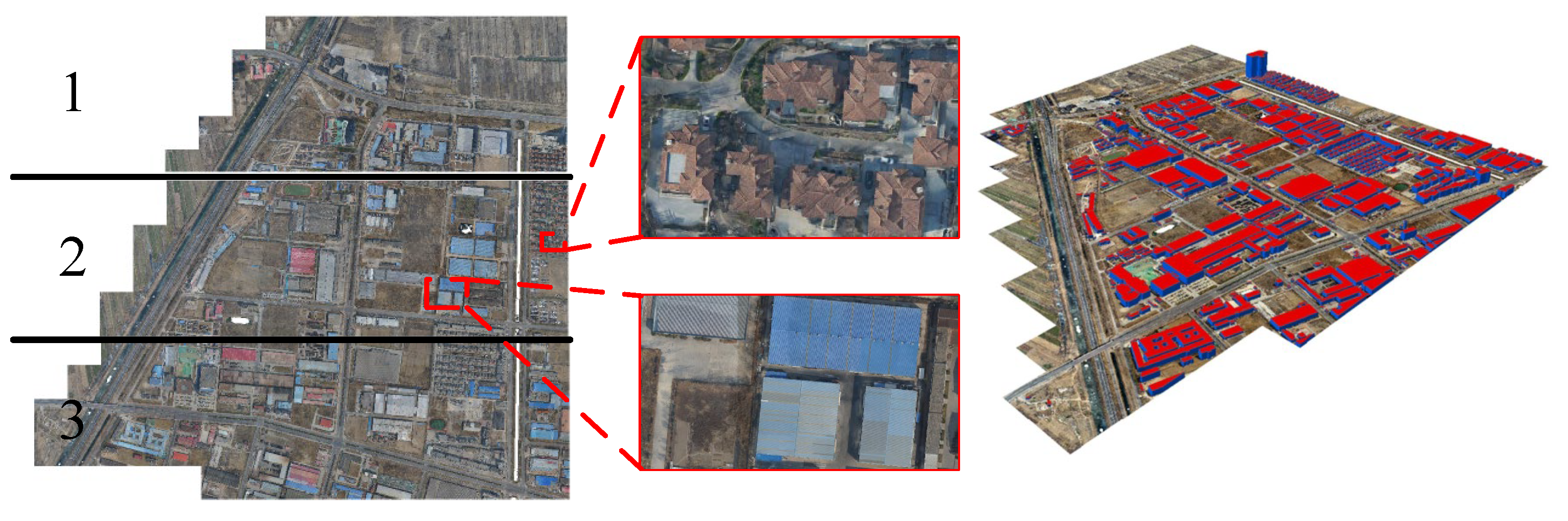
The Tianjin dataset [15] was collected in Tianjin, China, in an area consisting of two typical architectural styles—residential townhouses and industrial buildings—by using a drone-mounted camera to capture high-resolution images, and the captured photographs were used to obtain orthophotos and a DSM with a GSD of 0.1 m by using smart3D 2019 software with the MVS technique. The building boundaries were delineated in the orthophotos through a manual annotation method. The base and top elevations of each individual building were initially measured based on a statistical analysis of the building’s neighborhood elevation values which was then checked and edited manually to determine the building’s height. In this study, based on the classification method proposed in the original paper, images of Area 1 and Area 3 were used as the training set, which contained a total of 539 individual buildings; Area 2 was used for testing and validation and consisted of 243 buildings. Figure 9 shows the orthophotos and the corresponding 3D reconstruction model for the Tianjin dataset.

4.1.2. Urban 3D Dataset

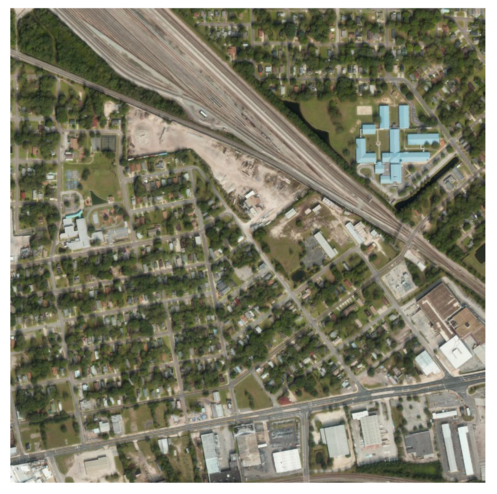
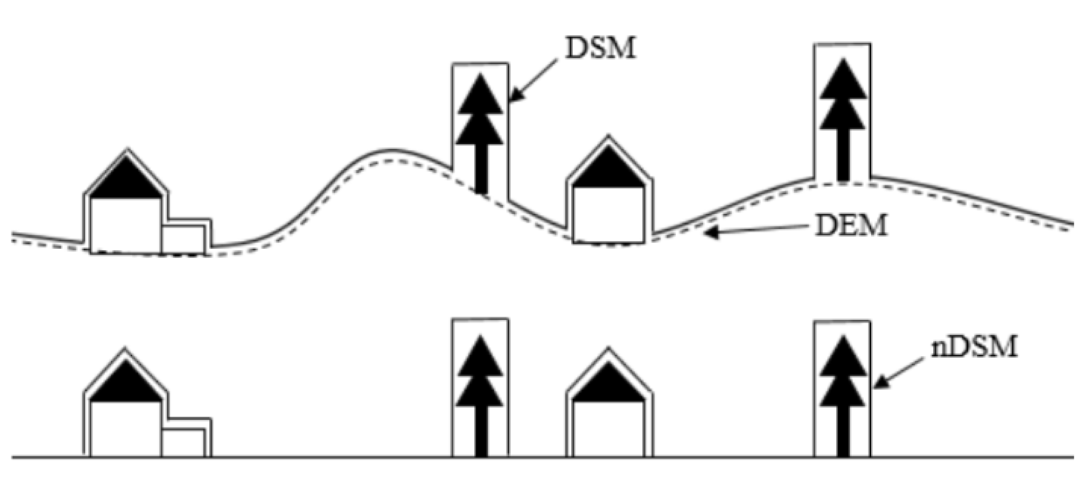
The Urban 3D dataset [37] was generated by the WorldView-3 satellite and contains RGB orthophotos and corresponding DSMs and DEMs. The data cover over 360 square kilometers of terrain and contain approximately 157,000 buildings, all with a GSD of 0.5 m. The dataset provides the true building footprint. This study uses a DSM to subtract the DEM to obtain the nDSM. Based on the real building footprint, the maximum value in that footprint is obtained from the nDSM as the verification value of the building height. Figure 10 shows an image of the Urban 3D dataset. The source images include a resolution of 2048 × 2048, of which 174 images are used for training and 62 images are used for verification and testing.

4.2. Evaluation Metrics

4.2.1. Building Footprint and Boundary Extraction

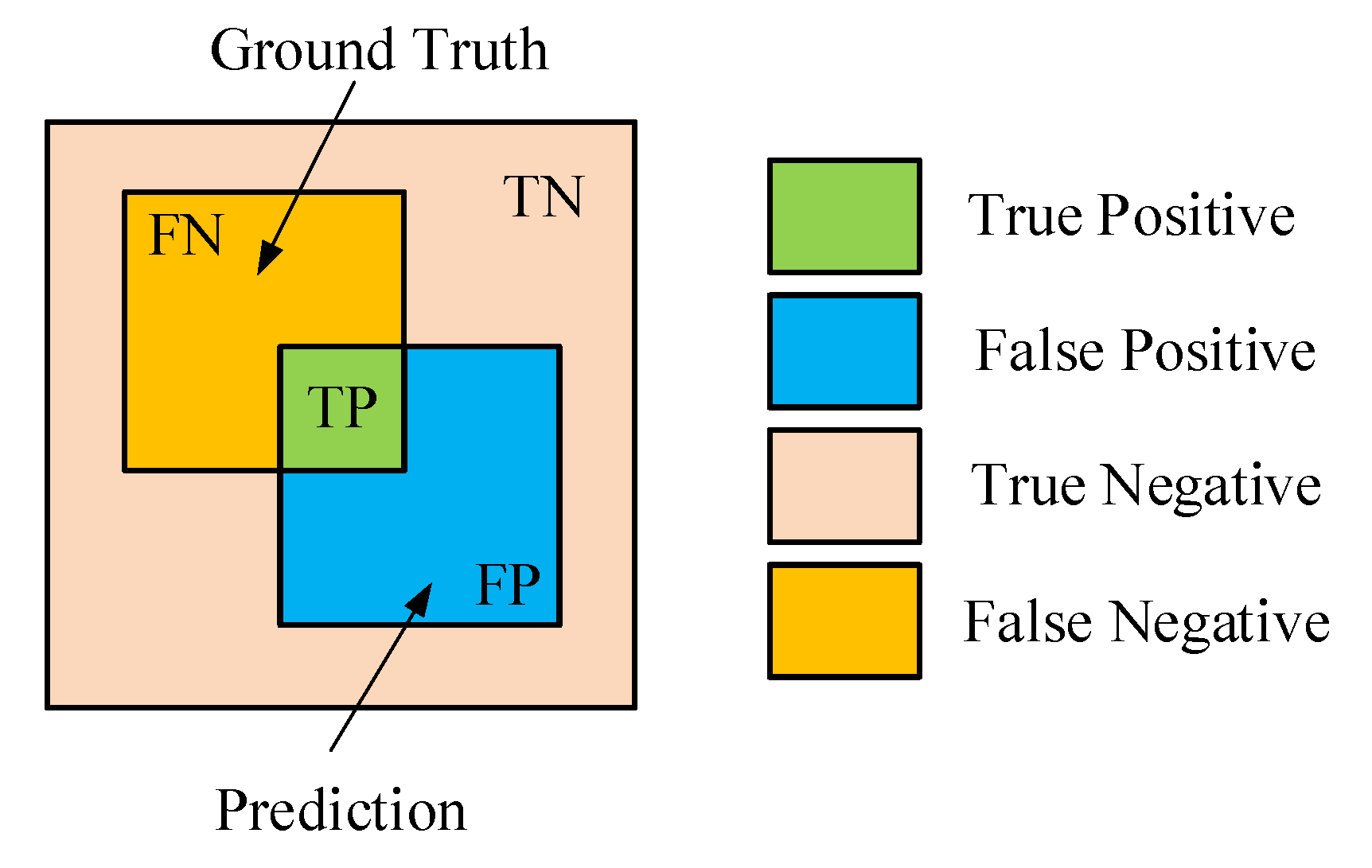
The semantic segmentation task is essentially a per-pixel-level classification task, and the confusion matrix, a standard tool for evaluating classification performance, contains four primary classification results: true positive (TP), true negative (TN), false positive (FP), and false negative (FN). The relationships of these concepts are shown in Figure 11.

In order to evaluate the effectiveness of building footprint and boundary extraction, this study adopted three performance metrics that are widely recognized in the industry: intersection over union (IoU), recall, and precision.

$$IoU=\frac{\mathrm{T}\mathrm{P}}{\mathrm{T}\mathrm{P}+\mathrm{F}\mathrm{P}+\mathrm{F}\mathrm{N}}$$

(2)

$$Recall =\frac{TP}{TP+FN}$$

(3)

$$Precision=\frac{\mathrm{T}\mathrm{P}}{\mathrm{T}\mathrm{P}+\mathrm{F}\mathrm{P}}$$

(4)

4.2.2. BIM Reconstruction

In order to evaluate the performance of the automated BIM reconstruction method that was proposed, the same evaluation metrics were used as in previous studies [15]. The accuracy of individual building reconstruction was first evaluated by using the 3D IoU, which was obtained by multiplying the IoU of the semantic segmentation of building footprints with the corresponding height IoU. Specifically, the cross-intersection between each extracted individual building footprint and its closest ground-truth building footprint was calculated to obtain the IoU of the building footprint’s semantic segmentation. The IoU height was the quotient of the predicted building height within a single building footprint and its closest ground-truth building height. After assessing the reconstruction accuracy for individual buildings, the effectiveness of the BIM reconstruction in the overall area was assessed using object-based completion metrics.

$$Correctness=\frac{\parallel TP\parallel }{\parallel TP\parallel +\parallel FP\parallel }$$

(5)

Here, TP represents the number of buildings with 3DIoU > 0.5 among all completed reconstructed buildings and FP represents the number of buildings with 3DIoU ≤ 0.5 among the reconstructed buildings.

4.3. Experimental Setup

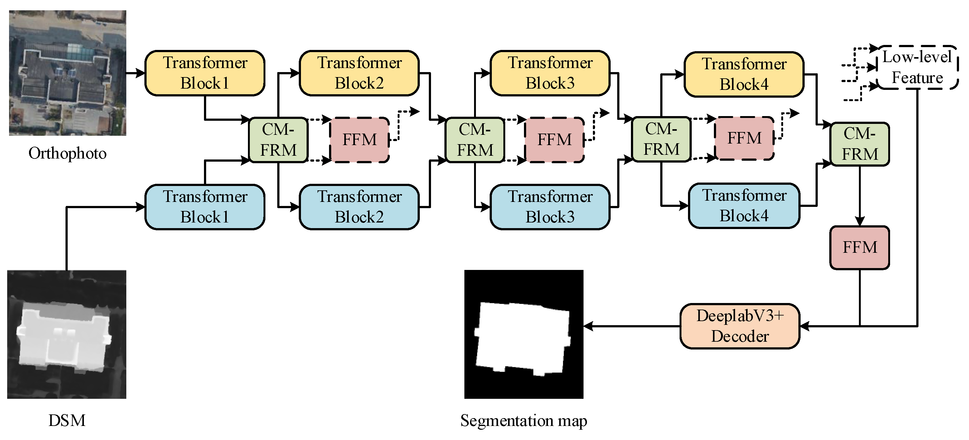
In the building footprint extraction phase, the performance of the model was highly dependent on the selection of hyperparameters. Through comparative analysis, we determined the optimal configuration. We adopted the Segformer model as the backbone of the semantic segmentation network and pre-trained it on the PASCAL VOC dataset, and we used mit-b2 for the pre-training weights. The other specific hyperparameter settings are shown in

Table 2. Configuration of hyperparameters.

Parameter	Operation Execution
Input size	512 × 512
Learning rate	6 × 10−5
Optimizer	AdamW
Loss	CrossEntropyLoss
Backbone	mit-b2
Epochs	100

.

In the boundary extraction stage, the parameters of the rules of thumb needed to be set manually; the GSD of the Tianjin and Urban 3D datasets corresponded to 0.1 m and 0.5, respectively, area thresholds of Td = 2000 and Td = 80 were defined to exclude buildings with an area of less than 20 square meters, length thresholds of Ts = 10 and Ts = 2 were set to exclude walls with a boundary length of less than 1 m, and α = π/6 was set to remove overly sharp nodes, whereas β = 17 π/18 was used to remove overly smooth nodes. During the height extraction stage, the maximum value of the nDSM within the boundary is used as the building height.

5. Results

5.1. Performance Analysis of Building Footprint Extraction

Table 3. Results of the Tianjin dataset.

Model	Backbone	Input Data	IOU (%)	Recall (%)	Precision (%)
DeeplabV3+	Xception	RGB	84.62	91.34	91.99
Segformer	Mit-b2	RGB	92.85	96.61	95.97
Unetformer	Swin-Base	RGB	94.13	97.11	96.85
SA-Gate	ResNet-50	RGB-D	94.78	97.06	97.59
CMX	mit-b2	RGB-D	96.71	98.57	98.08

and

Table 4. Results of the Urban 3D dataset.

Model	Backbone	Input Data	IOU (%)	Recall (%)	Precision (%)
DeeplabV3+	Xception	RGB	85.14	90.59	92.62
Segformer	Mit-b2	RGB	87.49	93.42	93.39
Unetformer	Swin-Base	RGB	89.92	93.98	95.07
SA-Gate	ResNet-50	RGB-D	90.08	94.23	95.68
CMX	mit-b2	RGB-D	92.78	94.57	96.06

compare the performances of different semantic segmentation models on the Tianjin dataset and Urban 3D dataset, respectively. In addition to the methods proposed in this study, the comparison also includes several models based on RGB data, such as DeeplabV3+, Segformer, and Unetformer, as well as the SA-Gate model, which uses RGB-D data. In the evaluation of the Tianjin dataset, the DeeplabV3+ model based on RGB data achieved 84.62% IoU, 91.34% recall, and 91.99% precision. Segformer, which uses Mit-b2 as the backbone network, improved the IoU to 92.85% while maintaining high recall and precision. Unetformer equipped with a Swin-Base backbone further improved the IoU to 94.13% and also showed simultaneous improvements in recall and precision. What cannot be ignored is that the inclusion of depth information has resulted in significant improvements in the performance indicators. The SA-Gate model with ResNet-50 as the backbone achieved an IoU of 94.78%. The CMX model used in this article, combined with a mit-b2 backbone and RGB-D data, achieved the highest IoU of 96.71%, as well as a very high recall rate (98.57%) and high precision (98.08%), demonstrating its excellent capabilities in semantic segmentation.

The evaluation of the Urban 3D dataset shows a similar trend, with the IoU of the DeeplabV3+ model based on RGB data being 84.64%. IoU and other performance metrics improve when using the Segformer and Unetformer networks. Consistent with the results of the Tianjin dataset, the fusion of the depth data significantly enhanced model performance, with the IoU of the SA-Gate model reaching 90.08%. What is particularly outstanding is that the CMX model used here reached 92.78% for the IoU, and the recall rate and precision were found to be 94.57% and 96.06%, respectively, which further confirms its effectiveness and reliability in extracting building outlines from satellite remote sensing data. DeepLabV3+, as the current benchmark segmentation method using a CNN, introduced the ASPP module into its encoder to enhance its capabilities at different scales and in structural feature extraction. SegFormer incorporates the strengths of the Transformer model, which performs well in dealing with global relations and long-distance dependencies in images, thus improving segmentation accuracy. Unetformer combines the advantages of CNNs and the Transformer model to achieve the best results when using RGB data. The multimodal fusion method using RGB-D data outperformed the methods using only RGB data in terms of the semantic segmentation results. This was because cross-modal fusion reduced redundant noise in a single modality and extracted complementary features. The DSM added in this study provided data about object elevation, which helped to distinguish among different buildings and improved the accuracy of building contours. The RGB-D data contained not only traditional RGB image data but also depth information, which enhanced the model’s spatial perception of objects in the scene.

Figure 12 illustrates examples of the building footprint segmentation results obtained by using different methods on an image with a resolution of 512 × 512, and the white pixels represent the building areas. It can be observed that the segmentation map obtained using CMX had the highest similarity with the real labeled map. In contrast, the segmentation map output by the DeeplabV3+ method was more complicated, and the result was different from the real labeling, whereas the segmentation map output by the Unetformer method only used RGB images, and the resulting map had holes inside the buildings. The segmentation figure obtained by the SA-gate method using RGB-D data had more precise edges, and the hole problem was solved. However, this method produced more segmentation errors due to the noise effect of DSM data. The CMX method used in this study achieved the optimal semantic segmentation results by effectively calibrating and extracting features from RGB images and DSM data.

5.2. Performance Analysis of Regularized Building Boundary Extraction

Table 5. Building boundary extraction results.

Method	IoU (%)
Semantic segmentation	96.71
Douglas–Peucker [23]	96.10
Polygon regularization algorithm [27]	92.13
Our method (polygon optimization)	95.07
Our method (polygon and empirical optimization)	95.92

presents the results of a quantitative evaluation that compares different regular building boundary extraction methods. The data in the table show that after using different methods to extract building boundaries from the semantic segmentation results, the IoU decreased. This phenomenon can be attributed to the fact that when simplifying the building outline, detailed information is omitted, affecting the IoU value. Nonetheless, appropriately reducing the IoU to obtain more regular building boundaries is a desirable trade-off strategy in terms of providing a more accurate structural basis for reconstruction. After the application of the Douglas–Peucker algorithm, although the IoU only dropped by 0.61%, further visual analysis shows that this algorithm is more limited during edge optimization tasks. As a common postprocessing method, the polygon regularization algorithm [27] can extract relatively regular building outlines, but it results in a significant decrease in IoU of 4.58%, indicating that this postprocessing method can be optimized. In the two-stage method proposed in this article, the polygon optimization stage caused the IoU to decrease by 1.64%, and combined with the experience optimization postprocessing stage, the IoU decrease was controlled at 0.79%. This confirms that this method retains high accuracy while simplifying building boundaries and also obtaining more regular building boundaries.

Figure 13 demonstrates the visual comparison results of building boundary extraction using different methods. The building boundaries extracted by the Douglas–Peucker algorithm [23] are relatively tortuous and have smaller edge differences than the semantic segmentation results, but there is a significant deviation from the regularized boundaries of the actual building. The building boundaries extracted by the polygon optimization method are more regular. However, due to the accuracy limitations of semantic segmentation itself, polygon optimization only plays a limited role in correcting semantic segmentation errors. As a result, errors still appear in the extraction results obtained using polygon optimization alone. For example, some areas that are too small are mistakenly extracted as buildings. In order to further optimize building boundaries and adapt them to the needs of BIM reconstruction, our method introduces the application of empirical optimization based on polygon optimization for adjustment, thereby obtaining more accurate regular building boundaries.

5.3. Performance Analysis of BIM Reconstruction

Table 6. Comparison of the different BIM reconstruction methods on the Tianjin dataset.

Method	$\mathbf{Correctness}$ (%)	$\mathbf{Correctness}$ (%)
	3DIoU > 0.5	3DIoU > 0.9
(Li et al., 2016) [38]	69.14	39.51
(Gui et al., 2021) [8]	74.14	43.21
(Yu et al., 2021) [15]	83.54	51.44
Our Method	85.61	56.44

and

Table 7. Comparison of the different BIM reconstruction methods on the Urban 3D dataset.

Method	$\mathbf{Correctness}$ (%)	$\mathbf{Correctness}$
	3DIoU > 0.5	3DIoU > 0.9
(Li et al., 2016) [38]	68.12	37.15
(Gui et al., 2021) [8]	72.27	39.32
(Yu et al., 2021) [15]	81.45	47.22
Our Method	82.93	53.57

compare the performance of different BIM reconstruction technologies on the Tianjin and Urban 3D datasets. Table 6 demonstrates the performance comparison of various BIM reconstruction technologies on the Tianjin dataset. The results show that the method proposed in this study achieved reconstruction correctness of 85.61% when the 3D IoU is greater than 0.5, and even under more stringent conditions; that is, when the 3D IoU was greater than 0.9, the correctness still remained at 56.44%. This method shows significant performance improvements compared to existing techniques reported in the literature.

The data in Table 7 reflect similar trends in the Urban 3D dataset. The method in this paper shows a correctness of 82.93% under a lower 3D IoU threshold (0.5) and a correctness of 53.57% under a higher 3D IoU threshold (0.9). This series of results continues to verify the consistent and excellent performance of this method in multiple datasets and further proves the feasibility of this technology in different urban environments.

The lower accuracy of architectural extraction when using traditional image-processing techniques [38] resulted in the lowest final reconstruction completion rate. The BIM reconstruction accuracy of this study’s method was also improved compared to the other deep-learning-based methods [8,15]. This improvement was mainly due to semantic segmentation using the multimodal fusion of orthophotos and DSMs in the building footprint extraction phase, which improved the accuracy of the building footprint extraction, and the postprocessing strategy designed for building boundaries obtained regularized building boundaries without drastically reducing the boundary accuracy.

6. Discussion

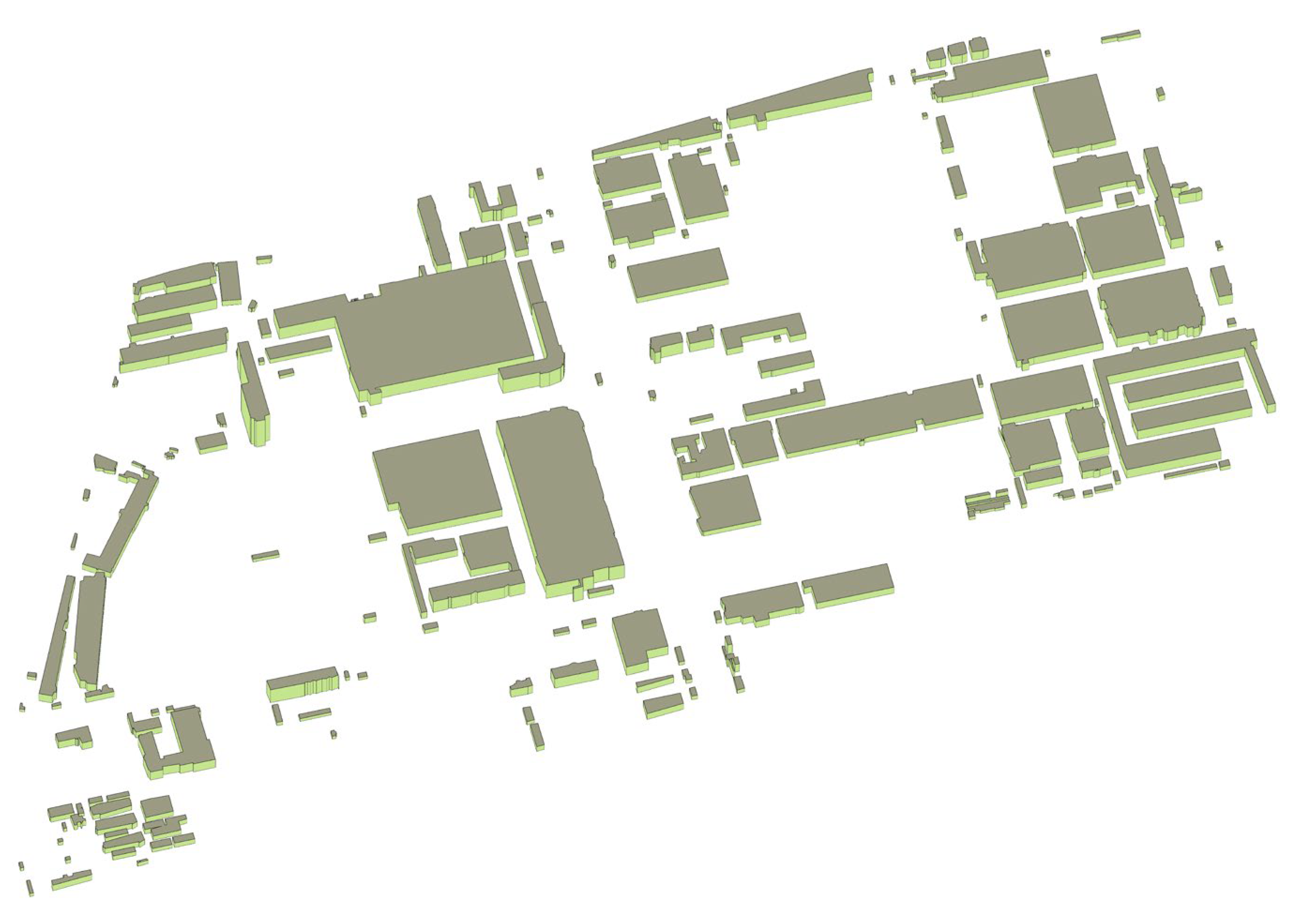
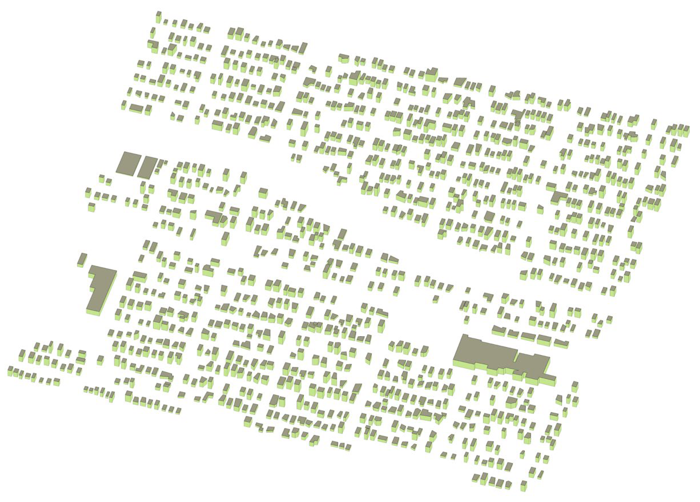
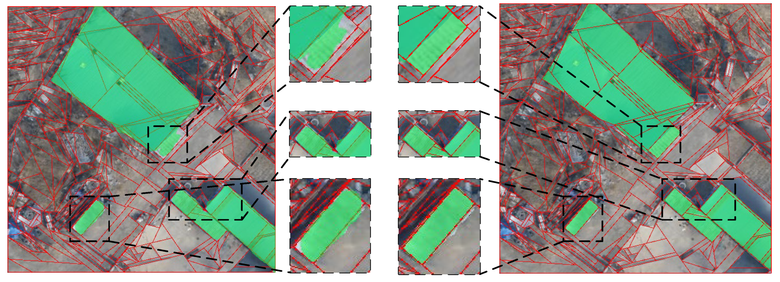
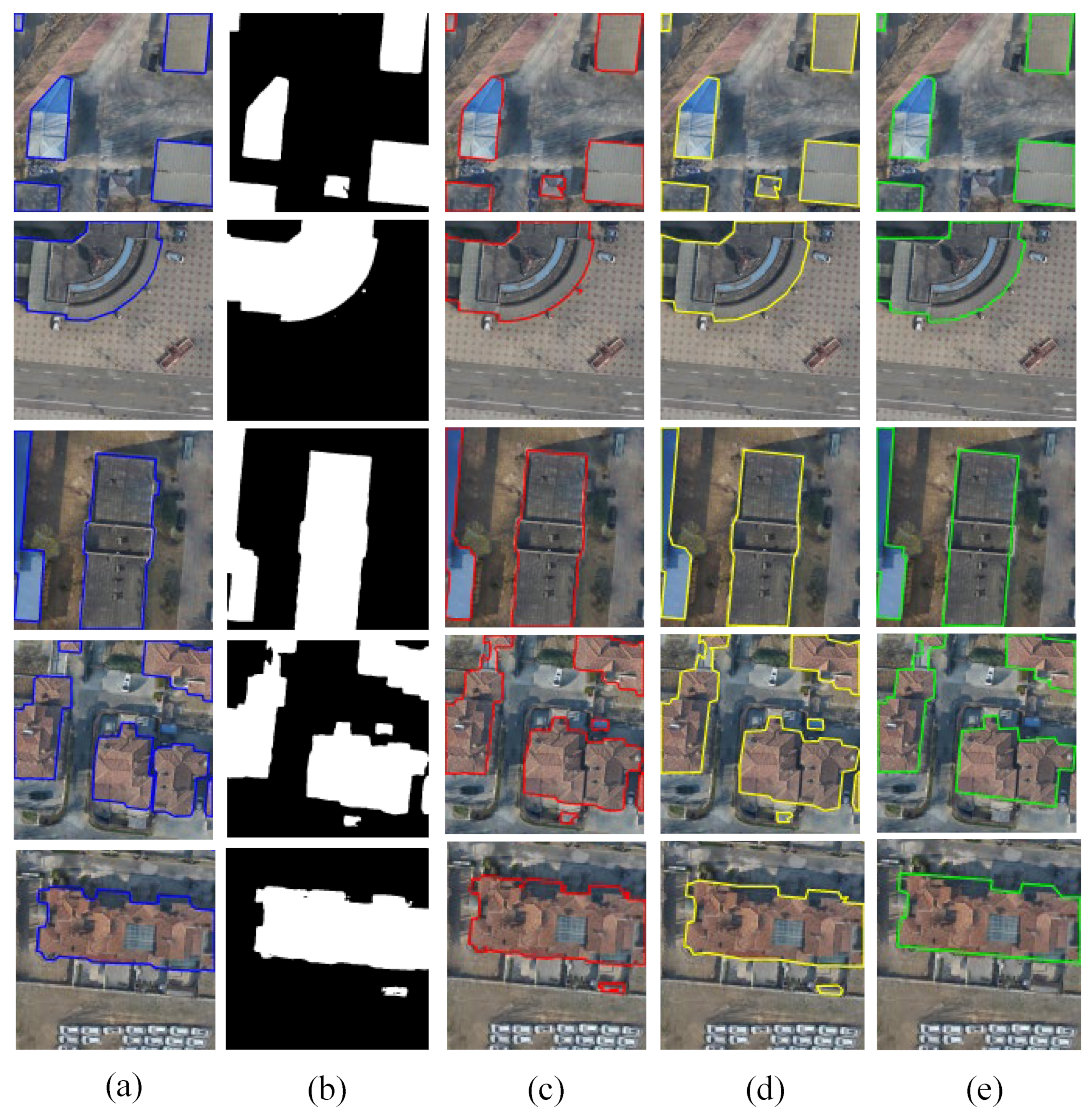
Figure 14 and Figure 15 demonstrate the results of this research method when applied to the reconstruction of a large-scale BIM. As can be seen in the figure, the BIMs reconstructed by applying this study’s method demonstrated neat building boundaries. Although there were errors in the reconstruction of some buildings, these could be corrected by a small amount of manual postprocessing. Compared with completely manual modeling methods, this method significantly reduces the need and time required for manual corrections and improves overall work efficiency.

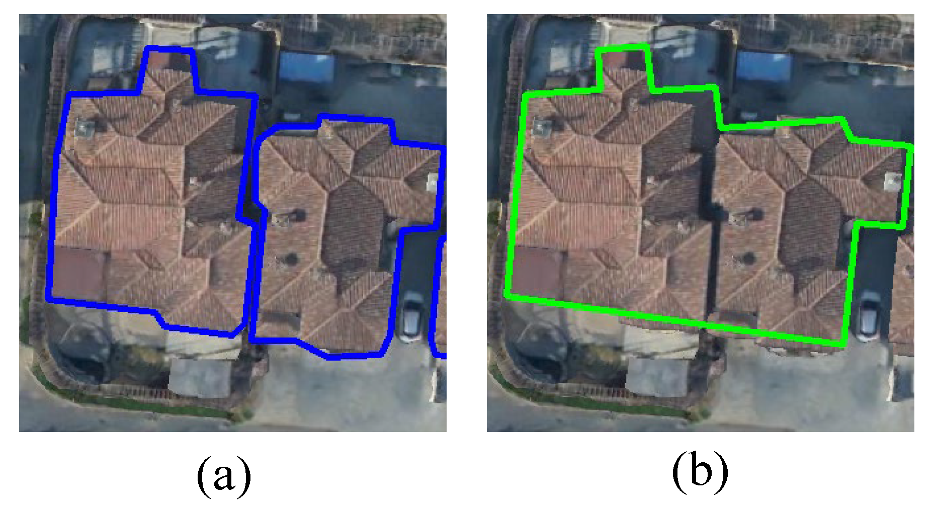
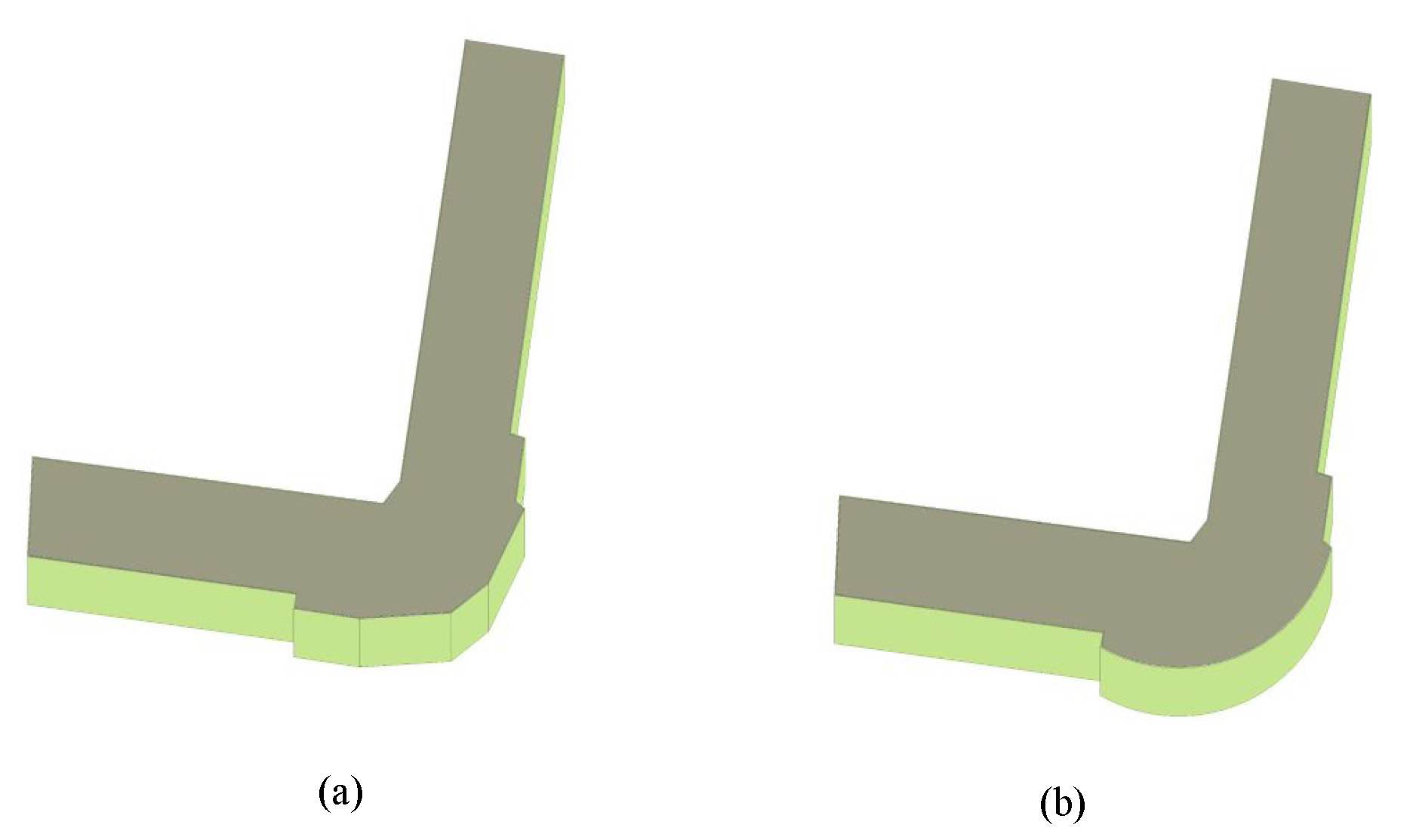
The proposed method can be effectively used to accomplish BIM reconstruction for most buildings, but it still has limitations in some cases as shown in Figure 16 and Figure 17. Due to the limitations of semantic segmentation, two closely adjacent buildings cannot be correctly separated in the initial stage, and two adjacent buildings may be recognized as one connected building, which will cause errors in the final BIM reconstruction; this can be solved by using instance segmentation in the future. In addition, the proposed regularized boundary extraction method is only applicable to regular and conventional buildings and will be simplified when dealing with buildings with circular boundaries.

In summary, the method proposed in this paper provides a feasible and highly accurate solution for large-scale BIM reconstruction, but it does have limitations in terms of the reconstruction of complex and irregular structures. The theoretical significance of this research lies in its regularized building contour extraction of orthophotos and DSMs through the CMX network and postprocessing-based approach, which helps to expand the idea of automated BIM reconstruction. Meanwhile, this research has important implications for the urban planning, facility management, and construction industries, where this automated, accurate BIM reconstruction approach can significantly increase efficiency and reduce costs.

7. Conclusions

In this study, an innovative approach to automated BIM reconstruction that utilized orthophotos with DSMs to achieve large-scale BIM reconstruction was proposed. The main conclusions are as follows.

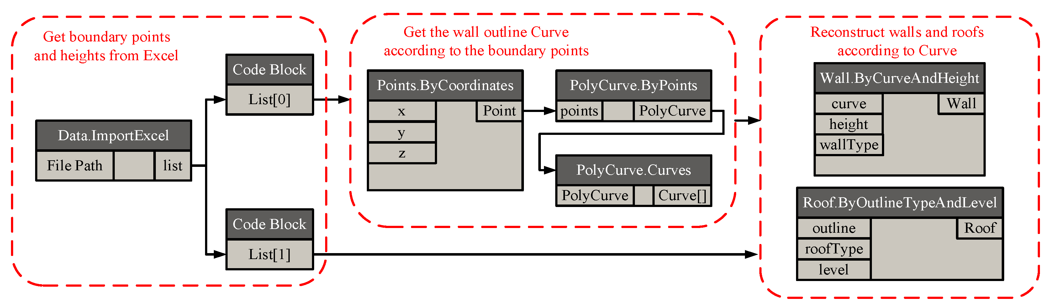
• The method proposed in this study is capable of obtaining regularized contour and elevation information of buildings from orthophotos and DSMs and of realizing automated batch reconstruction work by using Dynamo 2.1. The application to the Tianjin and Urban 3D datasets proved the effectiveness of the method, and the rate of correct reconstruction reached 85.61% and 82.93%, respectively. These results show that the method proposed in this paper represents a powerful tool for achieving high efficiency and high correctness during large-scale BIM reconstruction.
• In this study, it was verified that the CMX network can fully integrate the multimodal features of orthophotos and DOM for the semantic segmentation of building footprints, and the segmentation results were better than those of methods that used RGB. The IoU in building semantic segmentation with the CMX network reached 96.71% and 92.78% on the Tianjin and Urban 3D datasets, respectively. The significant improvement in this indicator sets a new benchmark for subsequent research.
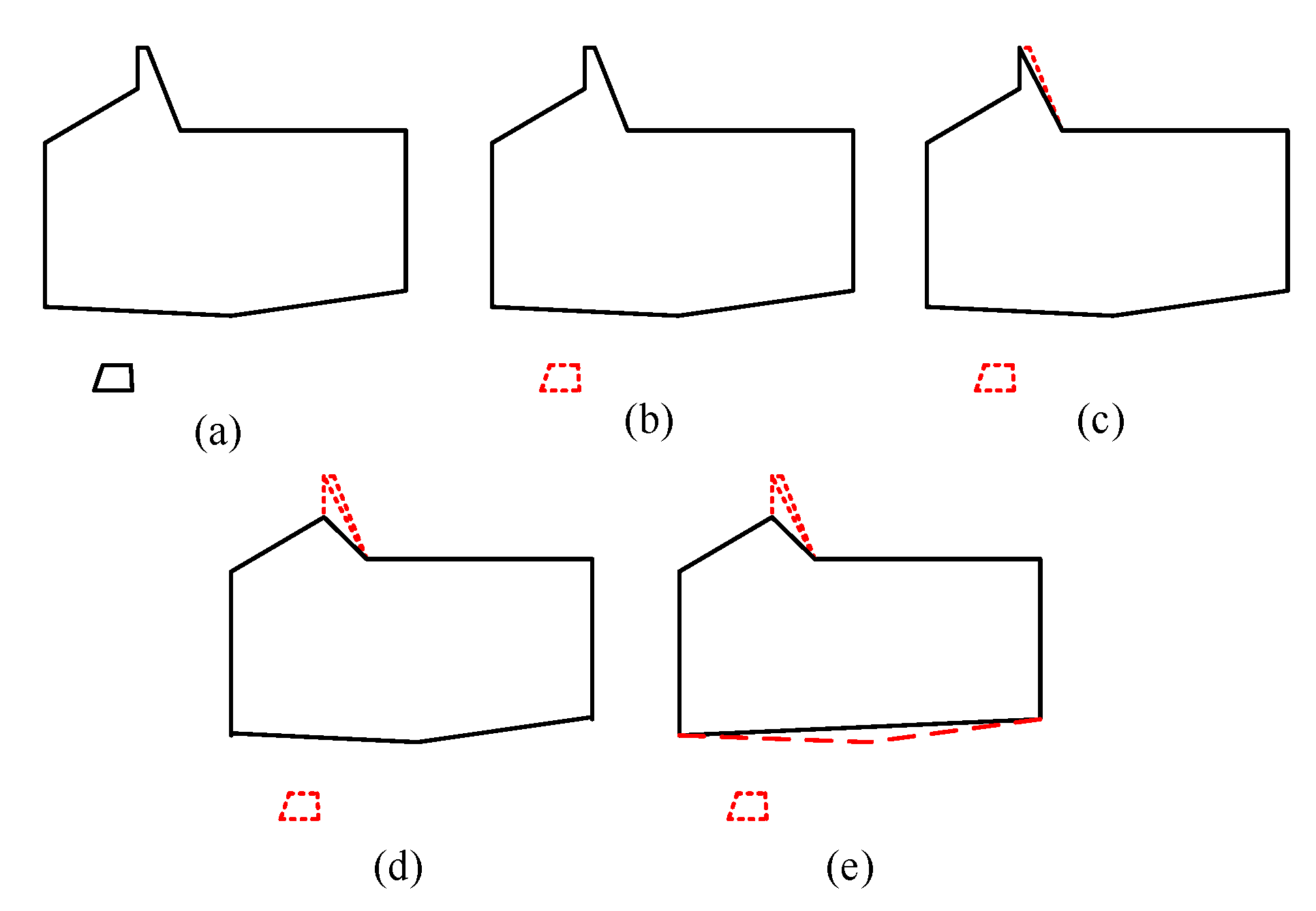
• The two-stage regular building boundary extraction method proposed in this study using polygon optimization and empirical rules for postprocessing semantically segmented images was able to accurately extract regularized building boundaries. It provides a new direction for subsequent regularized building boundary extraction.

The significance of this study is that it proposes a novel approach to large-scale BIM reconstruction. The method proposed in this paper can greatly reduce the time and labor required for traditional BIM reconstruction, thereby enabling more frequent updates of the BIM database and supporting the rapid development of smart city initiatives. Furthermore, the high accuracy of our reconstruction method can greatly improve the reliability of BIM data, which are crucial for urban planning, disaster management, and renovation projects.

The method proposed in this paper can complete building extraction and boundary optimization tasks. In addition, various advanced optimization algorithms [39,40] have previously been used as solutions in many fields such as scheduling [41,42] and optimization [43]. For the decision problem involved in this study, the method proposed in this paper can be compared with other advanced optimization algorithms in future research.