Author Contributions
Conceptualization, F.W. and L.M.; methodology, F.W. and L.M.; software, F.W. and L.M.; validation, F.W. and L.M.; formal analysis, F.W. and L.M.; investigation, F.W. and L.M.; resources, H.-G.M. and S.K.; data curation, F.W. and L.M.; writing—original draft preparation, F.W., L.M., H.-G.M., and S.K.; writing—review and editing, F.W., L.M., H.-G.M., and S.K.; visualization, F.W. and L.M.; supervision, H.-G.M. and S.K.; project administration, H.-G.M. and S.K.; funding acquisition, H.-G.M. and S.K. All authors have read and agreed to the published version of the manuscript.
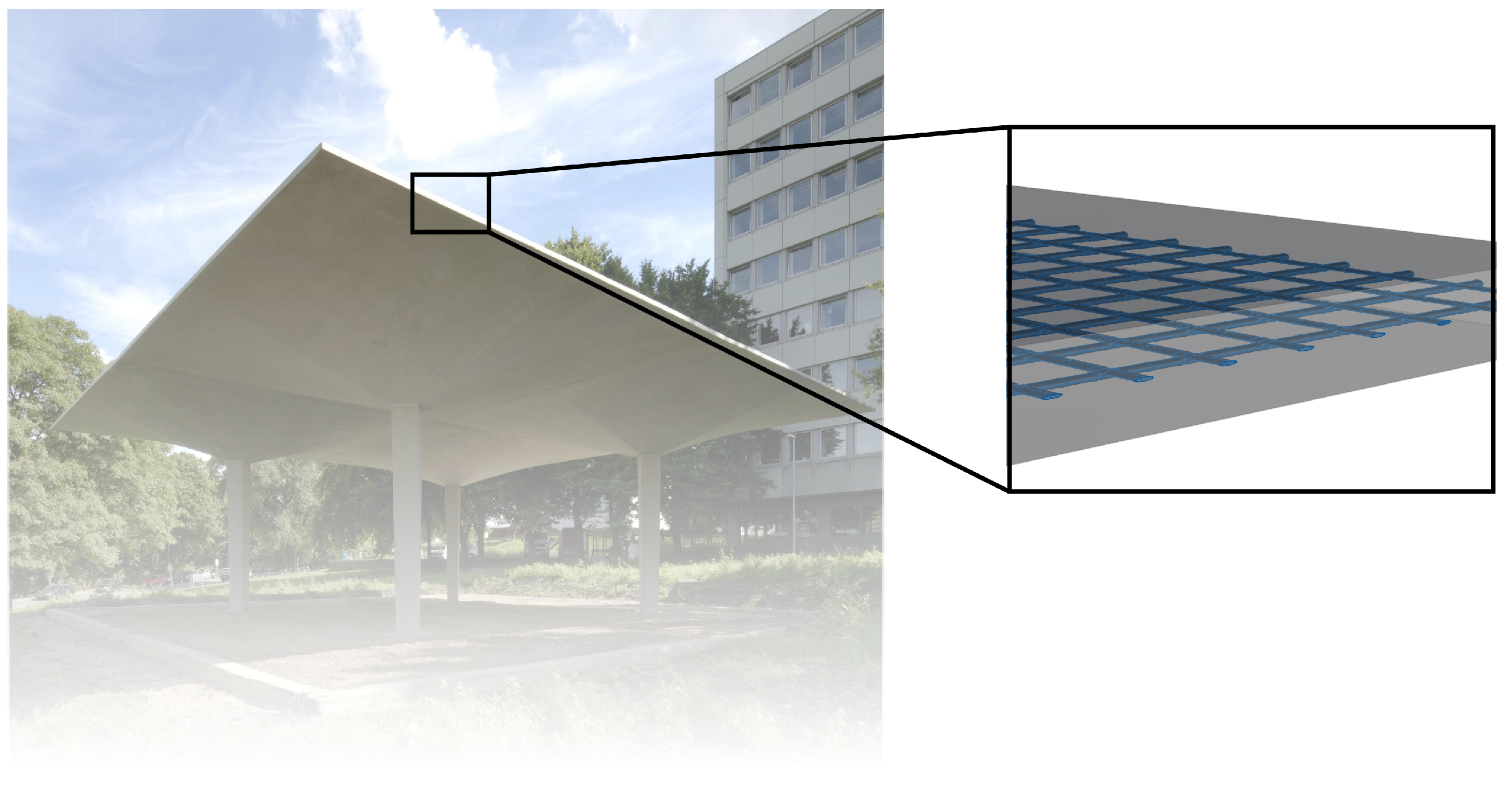
Figure 1.
Pavilion made from carbon reinforced concrete with example inner structure. The dimensions of each shell are 7 m × 7 m × 6 cm.
Figure 1.
Pavilion made from carbon reinforced concrete with example inner structure. The dimensions of each shell are 7 m × 7 m × 6 cm.
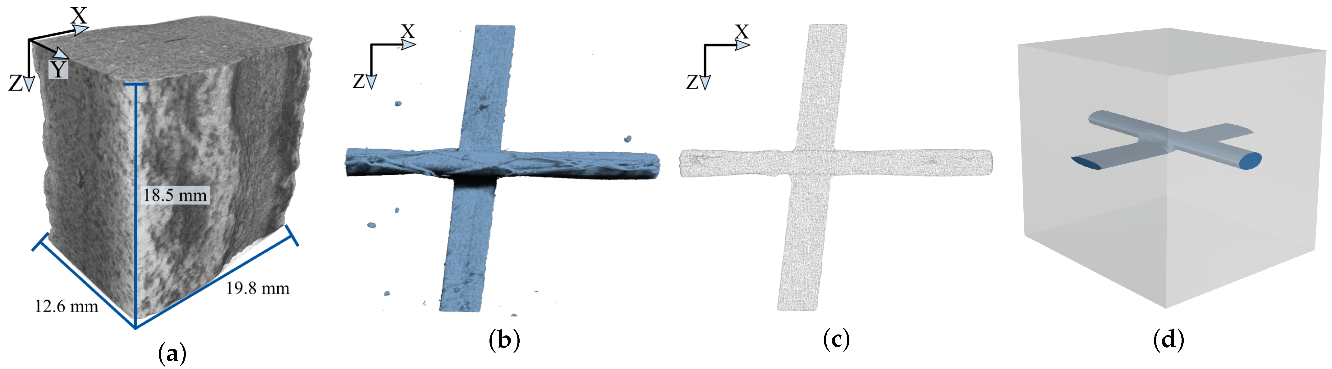
Figure 2.
From computed tomography (CT) reconstruction to representative volume element. (a) A CT reconstruction containing a carbon roving. (b) A segmentation of the roving contained in (a). (c) Point cloud representing solely the roving from (b). (d) Representative volume element including the carbon roving. (a,b) were visualized using Dragonfly 2021.1 by Object Research Systems (ORS).
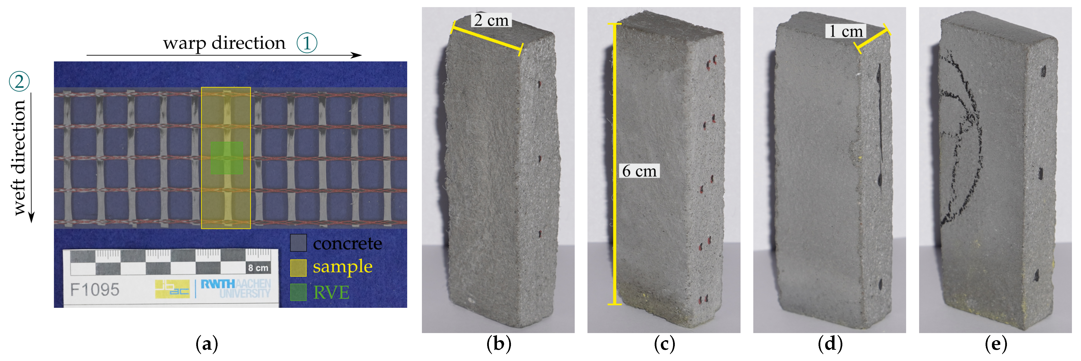
Figure 3.
(a) Scheme of the cut-out region of a sample (yellow) with Grid 1 and the dimensions of a representative volume element (green). The component is indicated by the gray overlay. (b–e) From left to right: Samples A, B, C, and D with carbon reinforcement (dark spots). All samples are of roughly the same size.
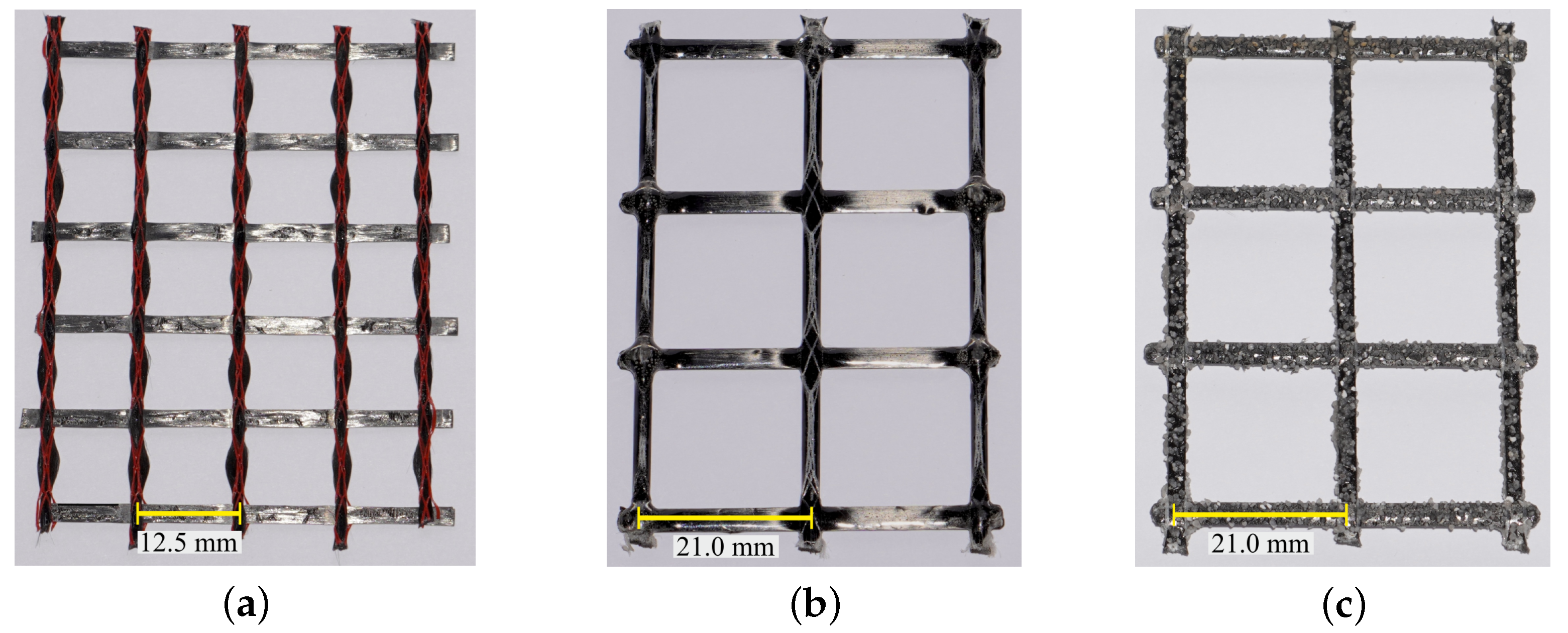
Figure 4.
(a) Grid 1 with knitting thread (red), (b) Grid 2 with knitting thread (white), (c) Grid 2 with sanded surface.
Figure 4.
(a) Grid 1 with knitting thread (red), (b) Grid 2 with knitting thread (white), (c) Grid 2 with sanded surface.
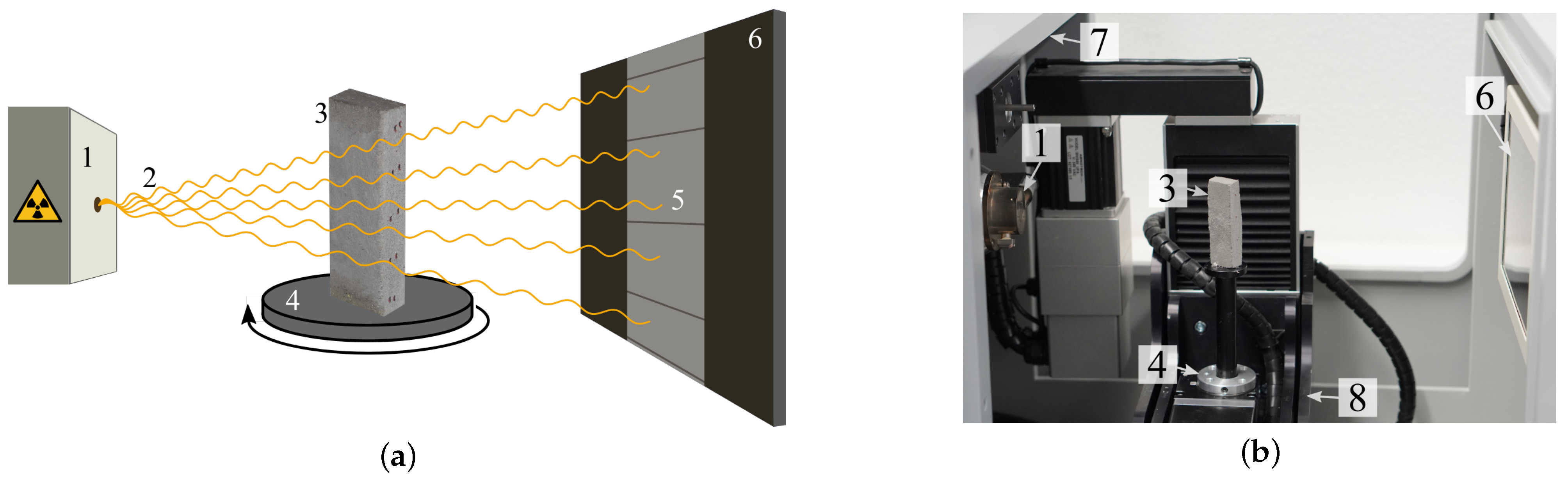
Figure 5.
Scheme and computed tomography (CT) device (Procon CT-XPRESS) with 1: X-ray source, 2: X-rays, 3: sample, 4: rotating sample plate, 5: projection on 6: X-ray detector, 7: protective cover (lead), 8: movable sample table. (a) Scheme of a CT device; (b) Photo of the test setup.
Figure 5.
Scheme and computed tomography (CT) device (Procon CT-XPRESS) with 1: X-ray source, 2: X-rays, 3: sample, 4: rotating sample plate, 5: projection on 6: X-ray detector, 7: protective cover (lead), 8: movable sample table. (a) Scheme of a CT device; (b) Photo of the test setup.
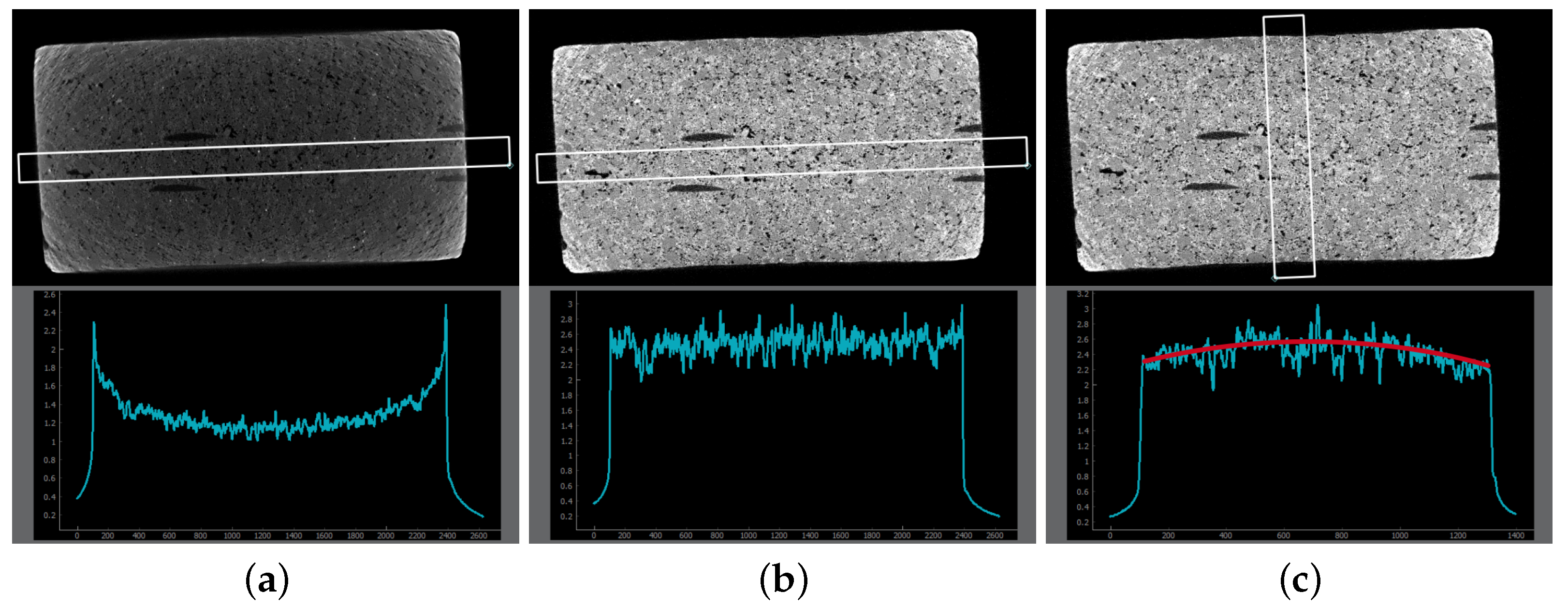
Figure 6.
Visualization of the beam hardening effect (cupping) and its correction during a computed tomography reconstruction process of Sample B using the reconstruction software X-AID 2023.2 (MITOS GmbH). Top: cross-sectional views; Bottom: grayscale profile. (a) Uncorrected reconstruction. The grayscale profile does not perfectly correlate with the specimen’s thickness. (b) Correction of the cupping effect along the long side of the sample. (c) Correction of the cupping effect along the short side of the sample using the values of (b). Due to differences in thickness between the long and short sides, the correction becomes too strong, resulting in a non-linear profile (the red line should ideally be straight).
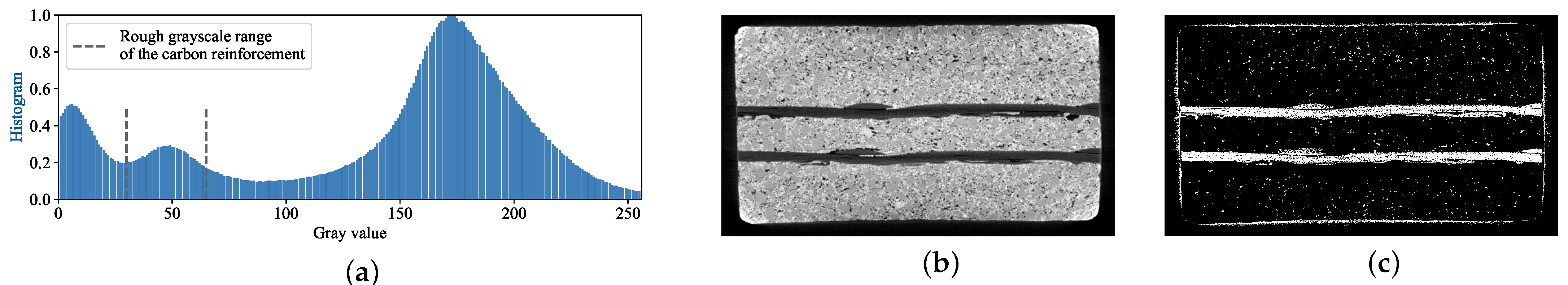
Figure 7.
(a) Normalized histogram of a cross-sectional image (b) of Sample B. The grayscale range of the carbon reinforcement is highlighted. (c) The horizontal slice (b) was used to calculate the histogram. A threshold was applied based on the grayscale range in (a). The result is a binarized image: all values outside the range were set to 0 (black), while all voxels inside the range were set to 255 (white).
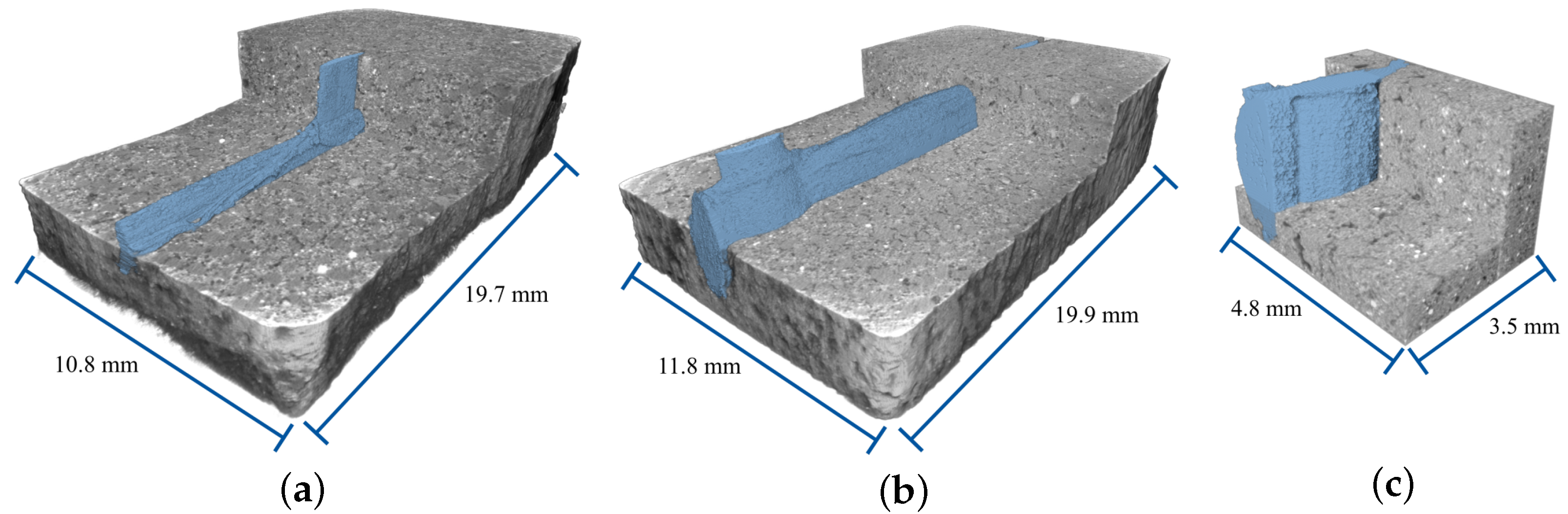
Figure 8.
Visualization of the Carbon Rovings Segmentation Dataset [
11] with manually segmented roving targets (light blue). The upper volumes have been reduced in depth to visualize the position of the rovings. (
a) Training volume of Textile 1. (
b) Training volume of Textile 2. (
c) Training volume of Textile 3. Volumes (
a) and (
b) were split into multiple subvolumes and represent the training and validation data. The volume in (
c) is used for testing. All textiles are variants of Grid 1 with different yarn spacings.
Figure 9.
Example visualization of a training subvolume of size 128 × 128 × 64 voxels (height × width × depth) before (a) and after applied online augmentation (b). From left to right: subvolume, related ground truth, and combined versions.
Figure 9.
Example visualization of a training subvolume of size 128 × 128 × 64 voxels (height × width × depth) before (a) and after applied online augmentation (b). From left to right: subvolume, related ground truth, and combined versions.
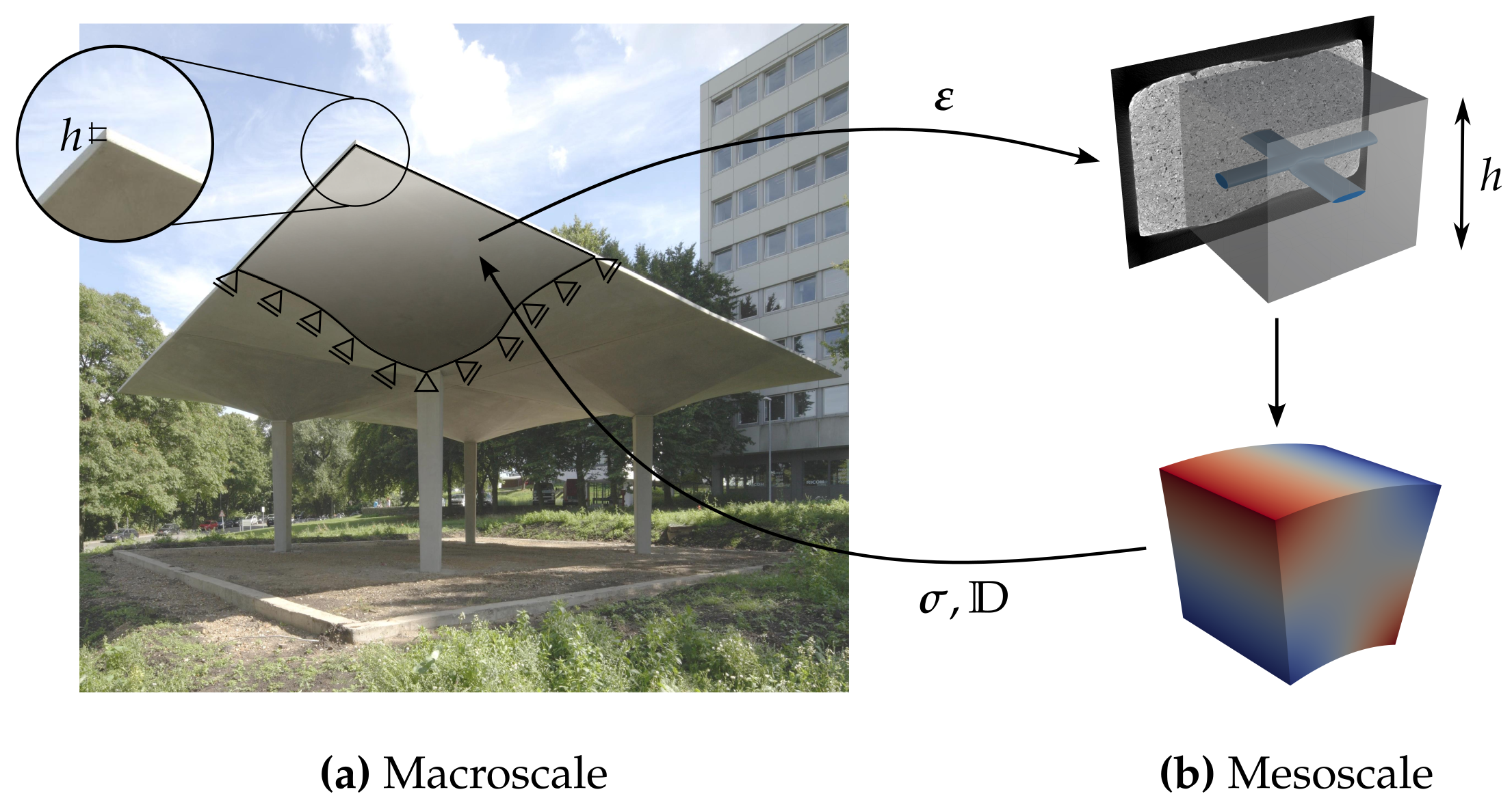
Figure 10.
Schematic homogenization procedure for shell structures using computed tomography data on the mesoscopic scale. (Adapted with permission from Ref. [
43]. 2023, L. Mester.)
Figure 10.
Schematic homogenization procedure for shell structures using computed tomography data on the mesoscopic scale. (Adapted with permission from Ref. [
43]. 2023, L. Mester.)
Figure 11.
(a) Exploded view of a cylinder and (b) example discretization of a section.
Figure 11.
(a) Exploded view of a cylinder and (b) example discretization of a section.
Figure 12.
(a) Perspective and (b) plane view (y–z plane) of parameterized RVE with dimensions (1: warp direction, 2: weft direction).
Figure 12.
(a) Perspective and (b) plane view (y–z plane) of parameterized RVE with dimensions (1: warp direction, 2: weft direction).
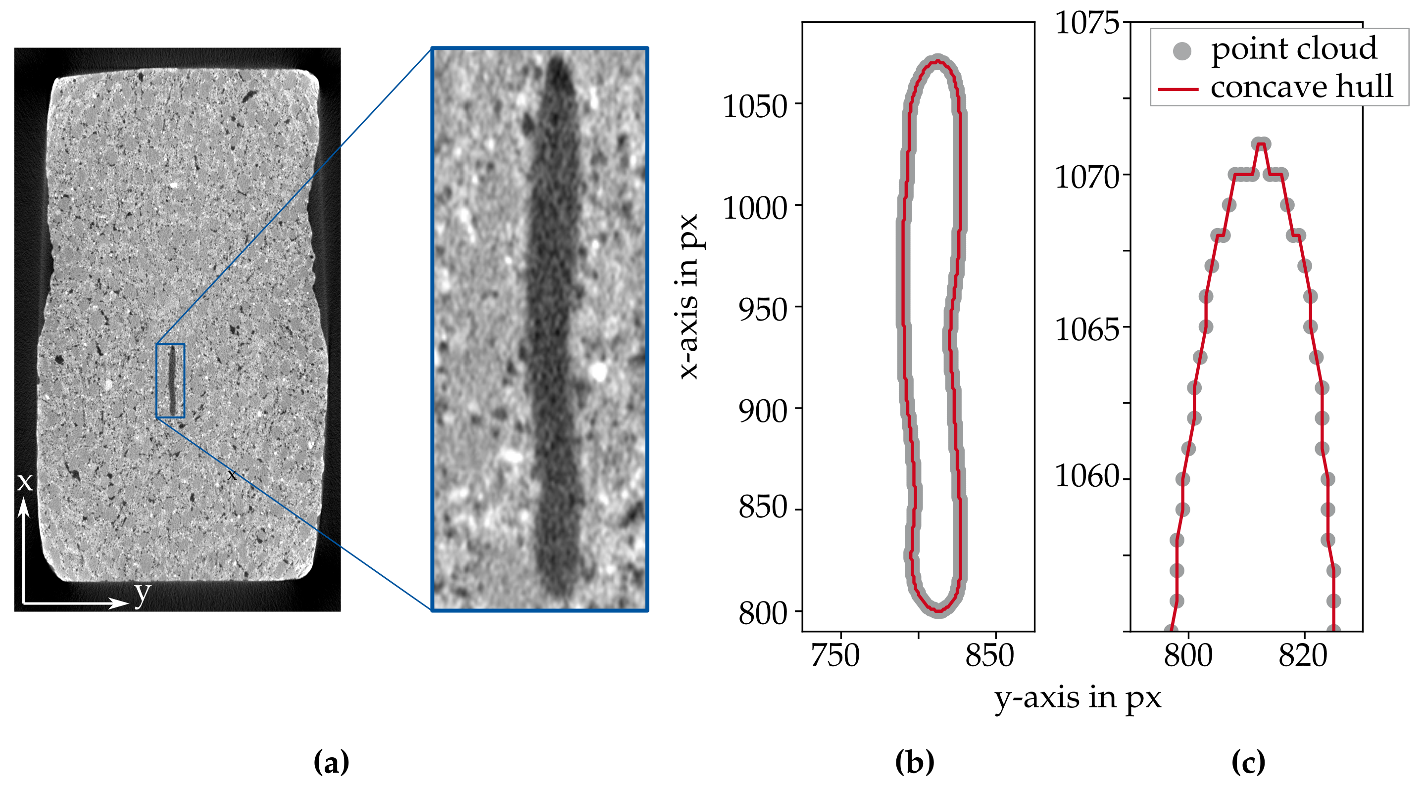
Figure 13.
(a) Example cross-sectional image of Sample A with magnification of roving. (b) Corresponding point cloud and concave hull. (c) Magnification of point cloud and concave hull.
Figure 13.
(a) Example cross-sectional image of Sample A with magnification of roving. (b) Corresponding point cloud and concave hull. (c) Magnification of point cloud and concave hull.
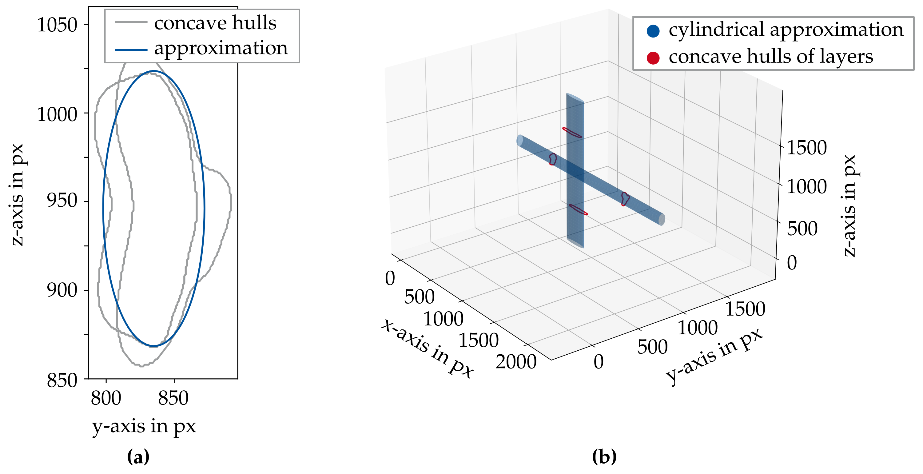
Figure 14.
(a) Plane view of approximated ellipse from two concave hulls describing the roving. (b) Perspective view of derived elliptical cylinders with concave hulls used for approximation.
Figure 14.
(a) Plane view of approximated ellipse from two concave hulls describing the roving. (b) Perspective view of derived elliptical cylinders with concave hulls used for approximation.
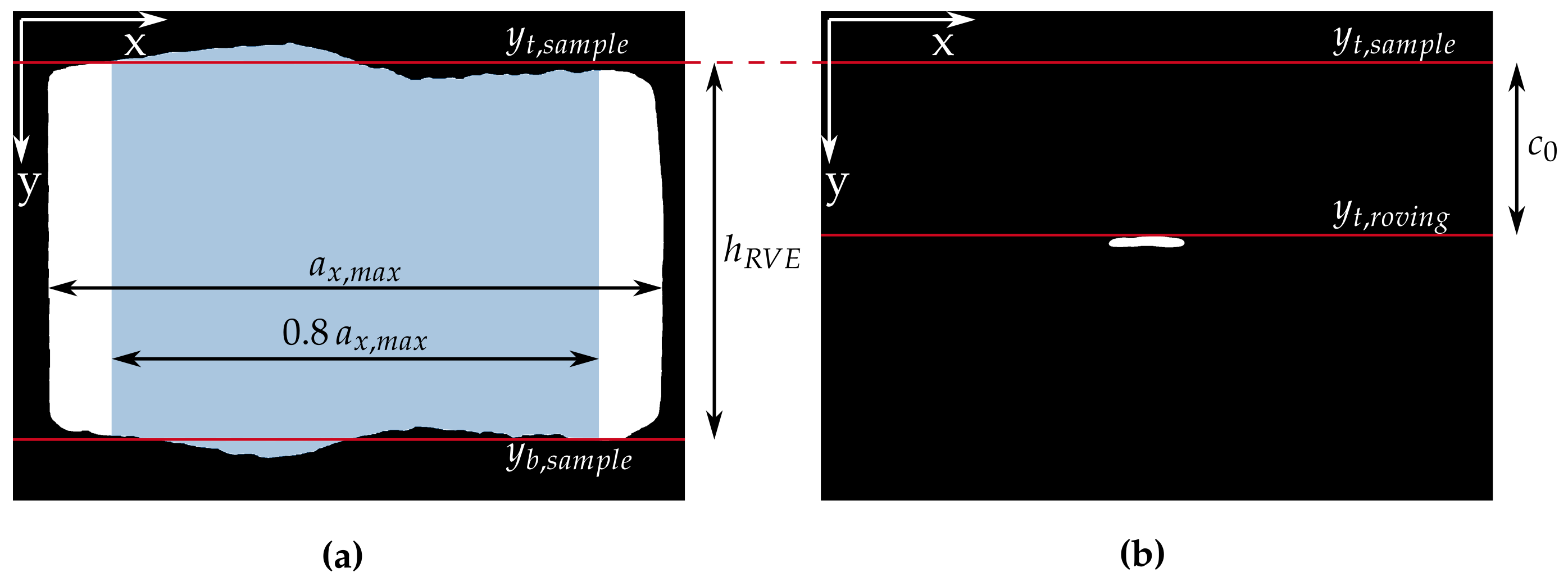
Figure 15.
(a) Binary image of Sample A (pixels belonging to sample have value 255 (white)). (b) Binary image of the roving contained in Sample A (pixels belonging to extracted roving have value 255 (white)).
Figure 15.
(a) Binary image of Sample A (pixels belonging to sample have value 255 (white)). (b) Binary image of the roving contained in Sample A (pixels belonging to extracted roving have value 255 (white)).
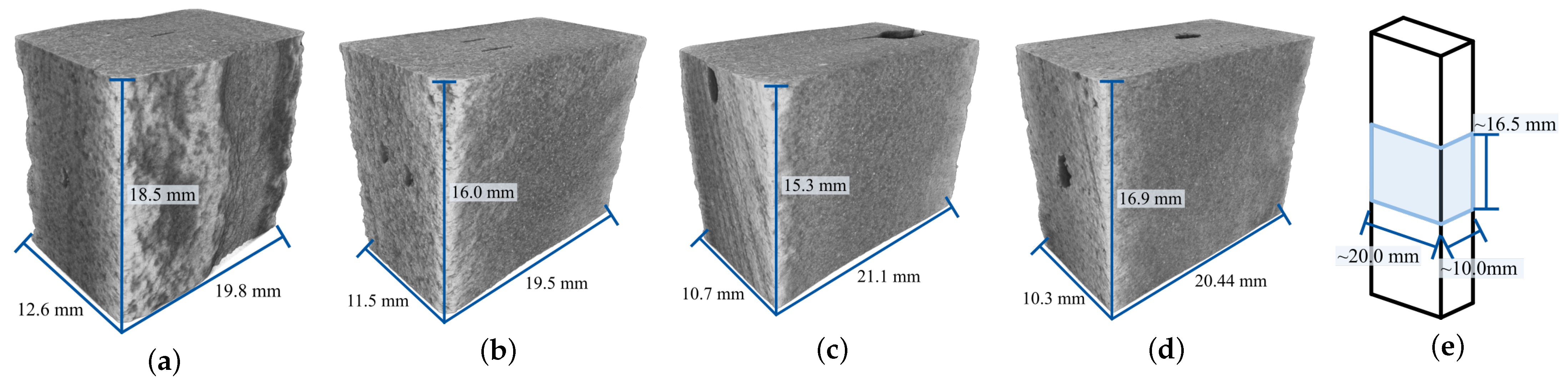
Figure 16.
(a) Sample A (voxel size: 9.5 µm). (b) Sample B (voxel size: 8.9 µm). (c) Sample C (voxel size: 9.4 µm). (d) Sample D (voxel size: 9.4 µm). The dark spots in the reconstructions are the carbon grids. (e) Schematic of the scanned region.
Figure 16.
(a) Sample A (voxel size: 9.5 µm). (b) Sample B (voxel size: 8.9 µm). (c) Sample C (voxel size: 9.4 µm). (d) Sample D (voxel size: 9.4 µm). The dark spots in the reconstructions are the carbon grids. (e) Schematic of the scanned region.
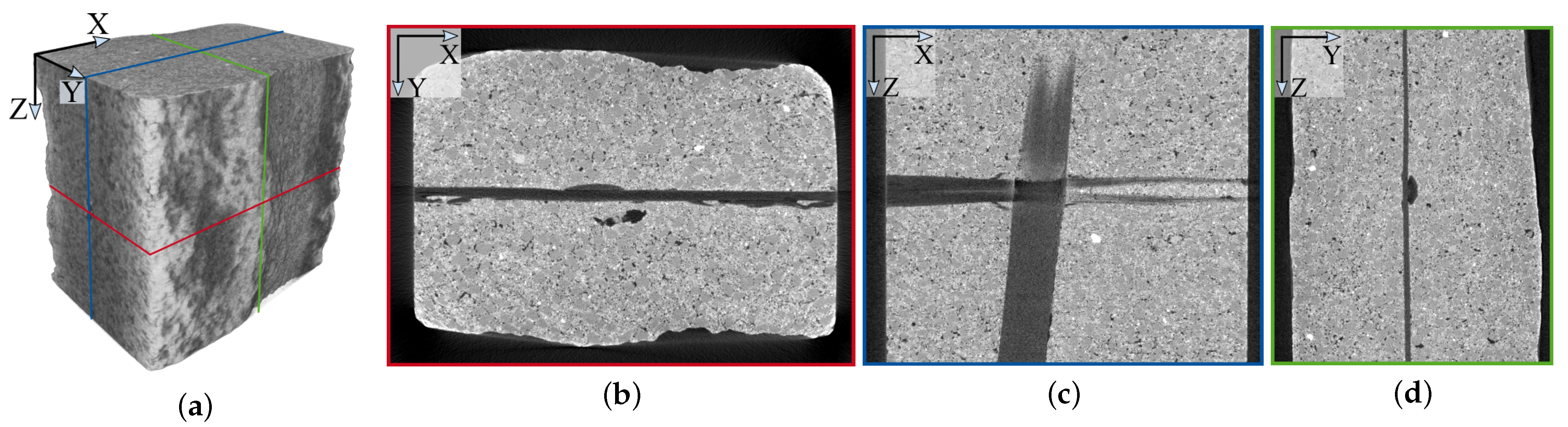
Figure 17.
Cross-sectional images of a computed tomography reconstruction of Sample A. (a) Sample A with marked image positions. (b) X–Y-view with roving. (c) X–Z-view with roving. (d) Y–Z-view with roving.
Figure 17.
Cross-sectional images of a computed tomography reconstruction of Sample A. (a) Sample A with marked image positions. (b) X–Y-view with roving. (c) X–Z-view with roving. (d) Y–Z-view with roving.
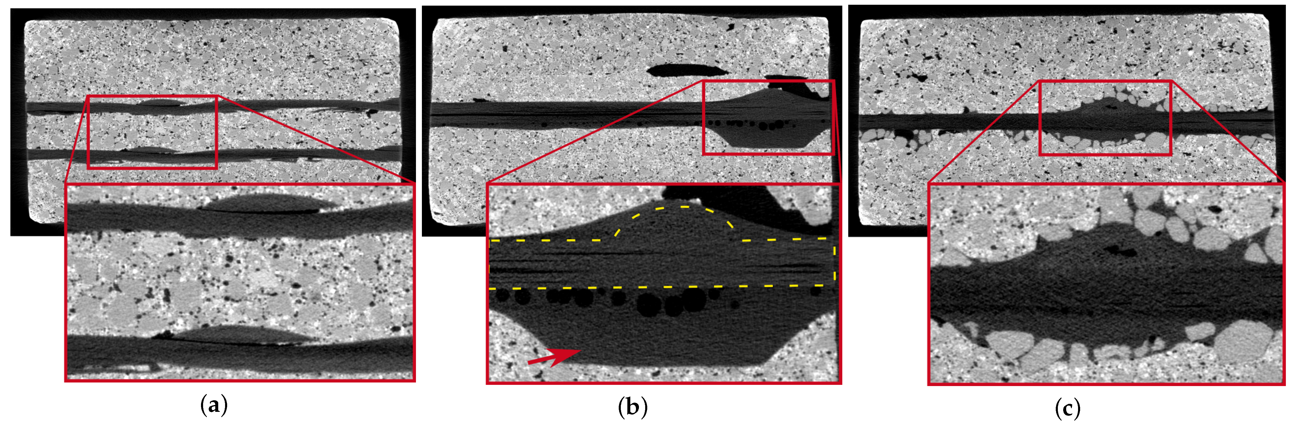
Figure 18.
Cross-sectional images of Samples B, C, and D along with magnifications. (a) Sample B contains a two-layer configuration of Grid 1. (b) Sample C contains Grid 2 with a lot of coating. The roving is highlighted within the yellow contours. The coating is indicated by the red arrow. (c) Sample D contains Grid 2 with a sanded surface, clearly visible in the computed tomography scan.
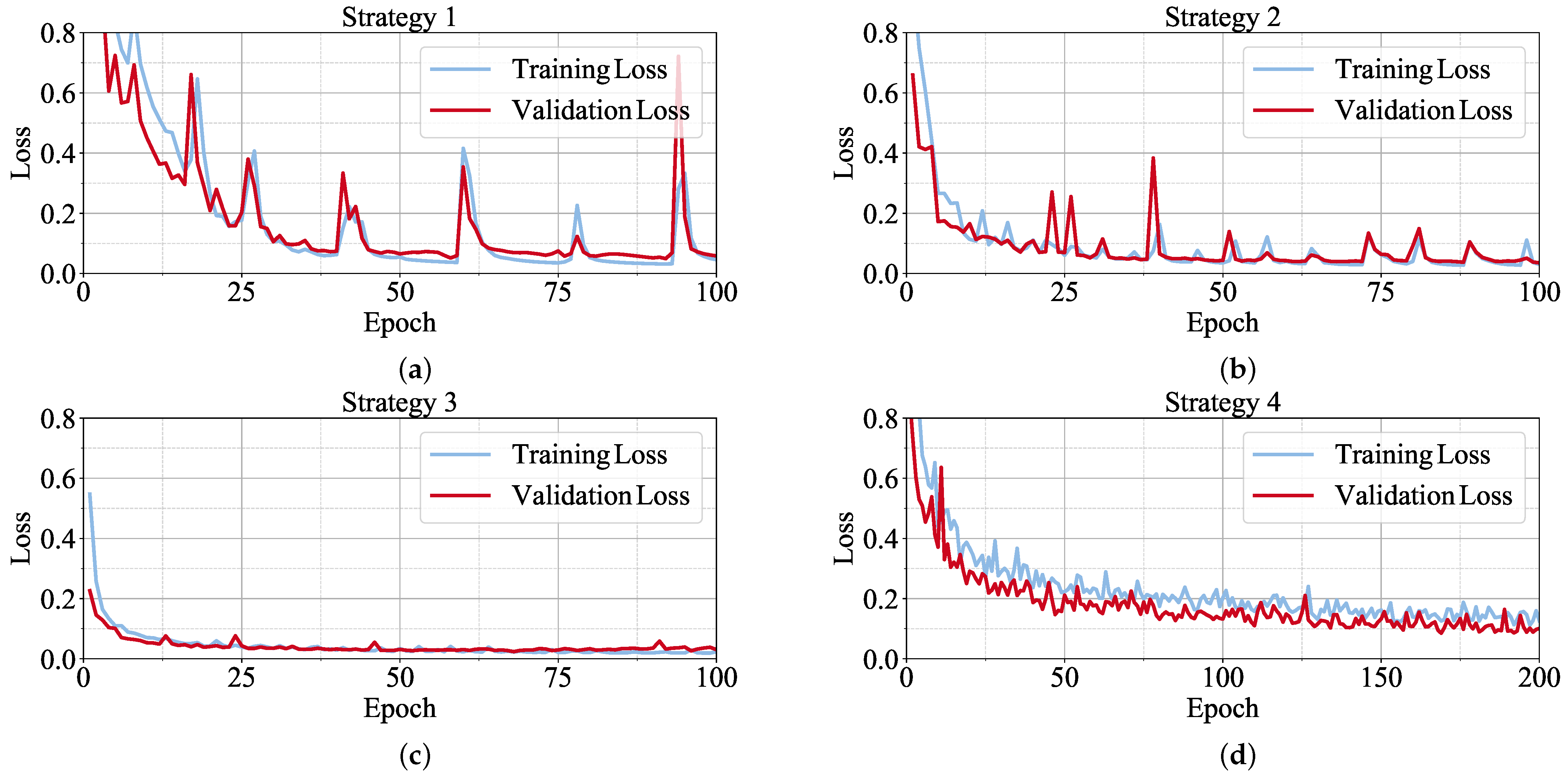
Figure 19.
Training and validation loss for all four strategies. (a) Strategy 1: No augmentation. (b) Strategy 2: Weak offline augmentation. (c) Strategy 3: Strong offline augmentation. (d) Strategy 4: Online augmentation.
Figure 19.
Training and validation loss for all four strategies. (a) Strategy 1: No augmentation. (b) Strategy 2: Weak offline augmentation. (c) Strategy 3: Strong offline augmentation. (d) Strategy 4: Online augmentation.
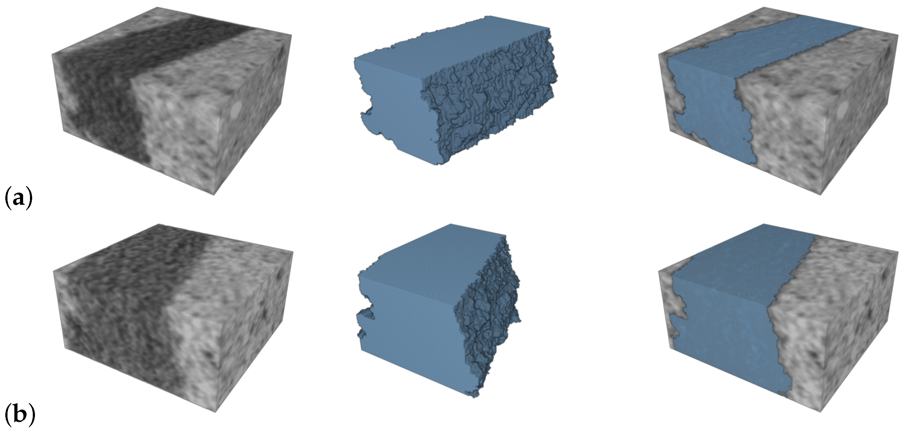
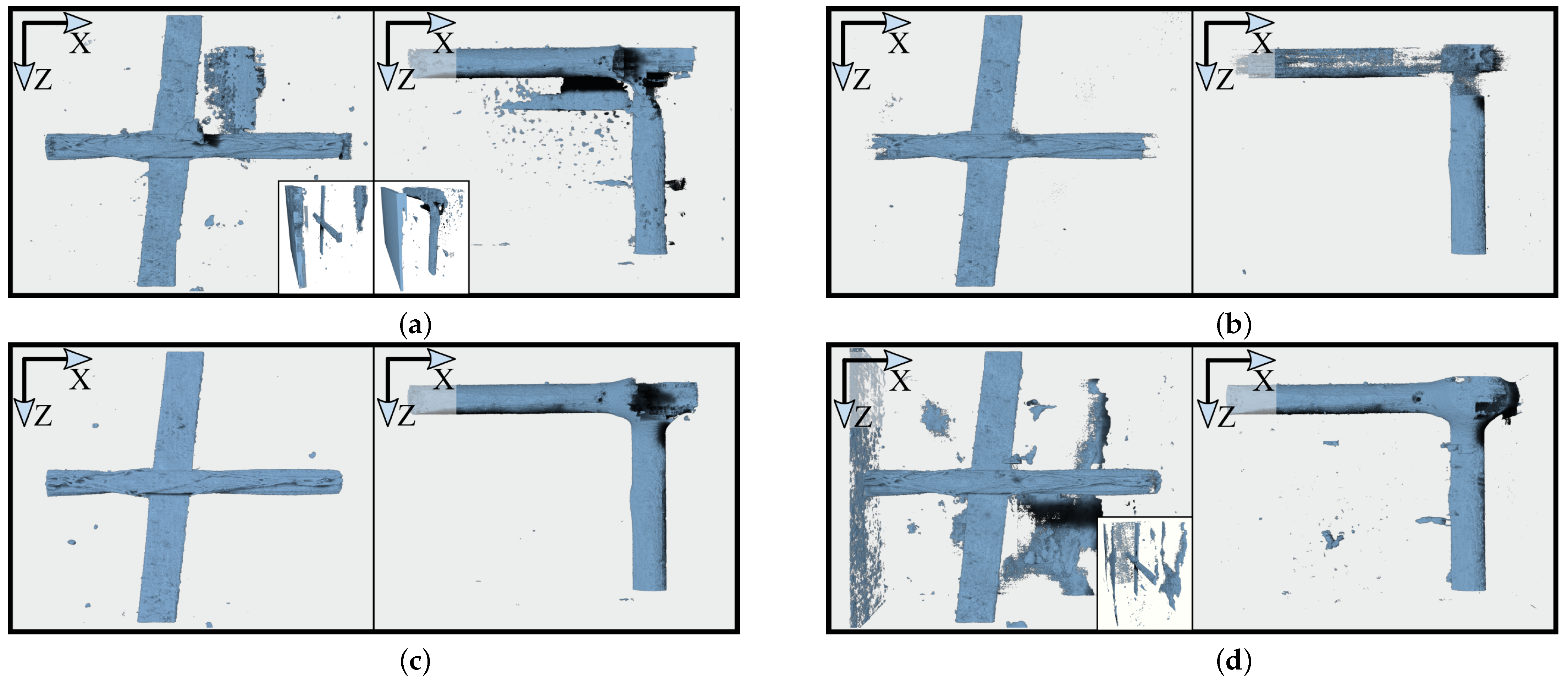
Figure 20.
Segmentation of Sample A (left in all subimages) and Sample C (right in all subimages) using each of the four strategies. (a) Strategy 1: No augmentation with removed artifacts in frontal views and full segmentation as miniatures. (b) Strategy 2: Weak offline augmentation. (c) Strategy 3: Strong offline augmentation. (d) Strategy 4: Online augmentation with removed artifacts in Sample A (frontal view) and full segmentation as miniatures.
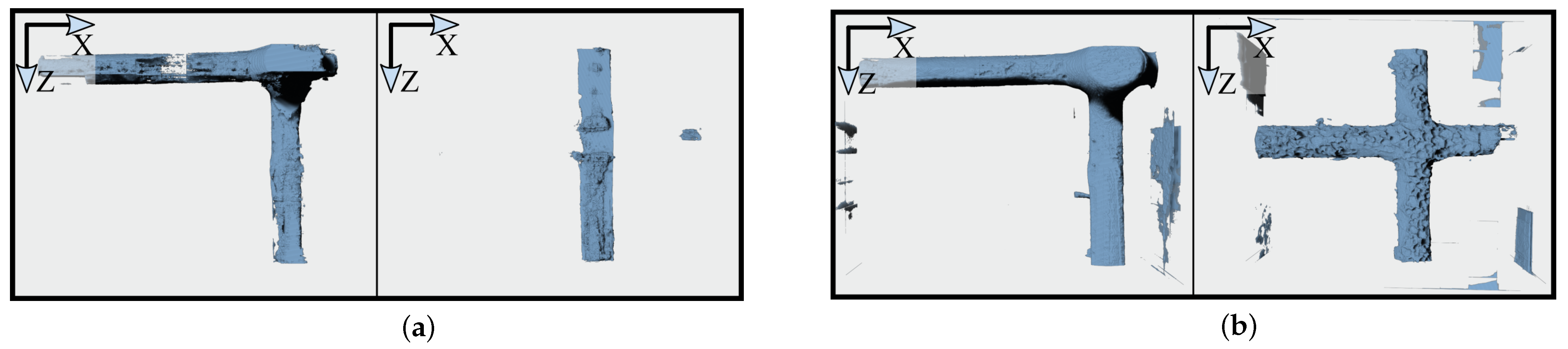
Figure 21.
Test of Strategies 3 and 4 on resized versions of Samples C and D (scale factor: 0.5, voxel size: 18.8 µm). (a) Strategy 3 on resized Samples C (left) and D (right). (b) Strategy 4 on resized Samples C (left) and D (right).
Figure 21.
Test of Strategies 3 and 4 on resized versions of Samples C and D (scale factor: 0.5, voxel size: 18.8 µm). (a) Strategy 3 on resized Samples C (left) and D (right). (b) Strategy 4 on resized Samples C (left) and D (right).
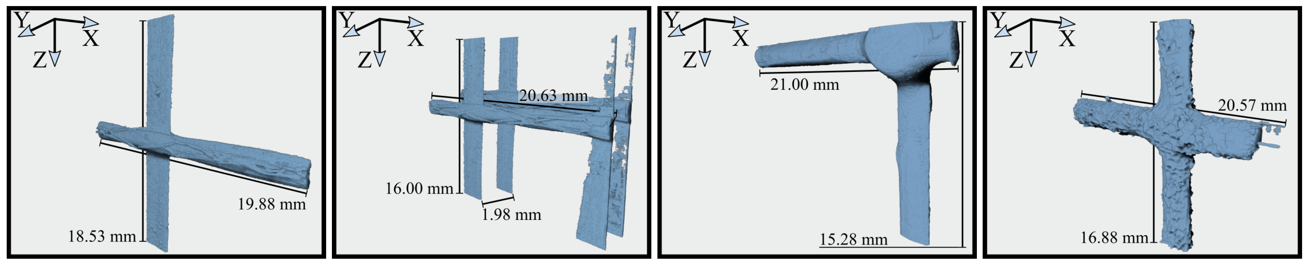
Figure 22.
Post-processed rovings using the 3D U-Net trained with Strategy 4. From left to right: Samples A, B, C, and D.
Figure 22.
Post-processed rovings using the 3D U-Net trained with Strategy 4. From left to right: Samples A, B, C, and D.
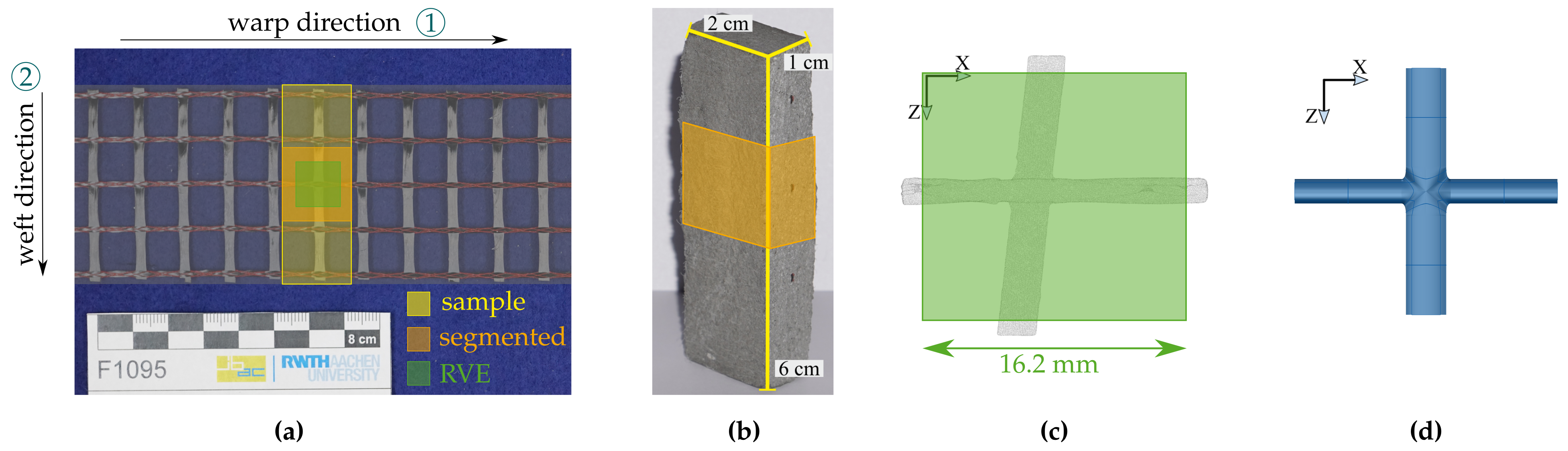
Figure 23.
(a) Textile of Sample A indicating the sample, segmented size, and size of representative volume element (RVE). (b) Sample A with highlighted scanned region. (c) Point cloud representing the roving in (a), RVE size indicated. (d) Surface model of the roving from the parameterized RVE.
Figure 23.
(a) Textile of Sample A indicating the sample, segmented size, and size of representative volume element (RVE). (b) Sample A with highlighted scanned region. (c) Point cloud representing the roving in (a), RVE size indicated. (d) Surface model of the roving from the parameterized RVE.
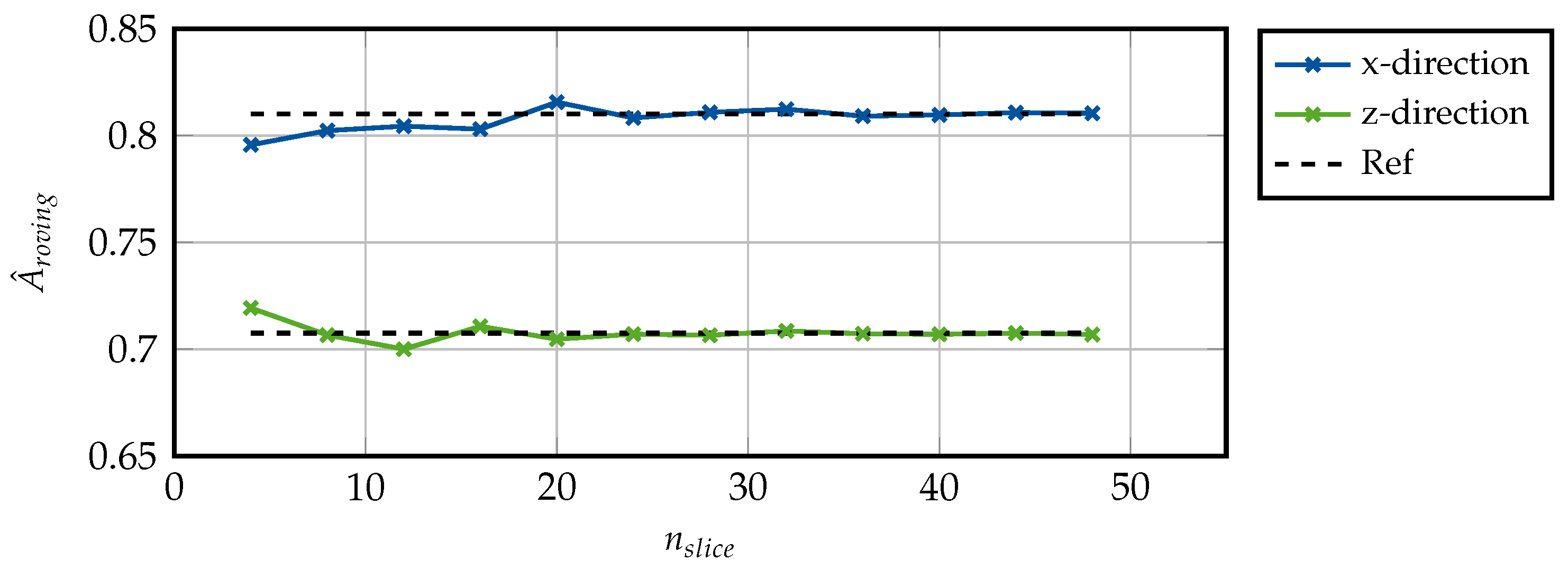
Figure 24.
Obtained cross-sectional area of roving for varying number of slices for each direction of Sample A.
Figure 24.
Obtained cross-sectional area of roving for varying number of slices for each direction of Sample A.
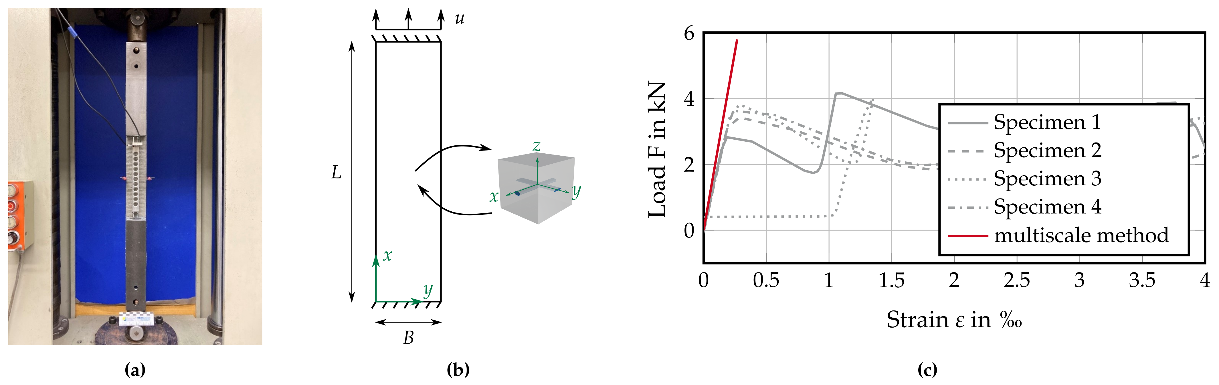
Figure 25.
(
a) Experimental setup. (
b) Adaptation for multiscale approach. (
c) Load-strain curve for tensile test. (Adapted with permission from Ref. [
65]. 2023, L. Mester).
Figure 25.
(
a) Experimental setup. (
b) Adaptation for multiscale approach. (
c) Load-strain curve for tensile test. (Adapted with permission from Ref. [
65]. 2023, L. Mester).
Table 1.
Measured cross-sectional dimensions of the rovings contained in Grid 1 and Grid 2. At the intersection of the rovings in the warp and weft directions, Grid 1 has a height of ≈0.88 mm, and Grid 2 has height of ≈3.15 mm due to the coating.
Table 1.
Measured cross-sectional dimensions of the rovings contained in Grid 1 and Grid 2. At the intersection of the rovings in the warp and weft directions, Grid 1 has a height of ≈0.88 mm, and Grid 2 has height of ≈3.15 mm due to the coating.
| Roving | Fiber Strand Grid 1 | Fiber Strand Grid 2 |
|---|
| | Height in mm | Width in mm | Height in mm | Width in mm |
| Warp direction | 0.55 | 1.41 | 1.41 | 2.13 |
| Weft direction | 0.29 | 2.35 | 1.02 | 2.51 |
Table 2.
Computational time required to process 100 epochs, depending on the augmentation strategy. The dataset used for online augmentation has been increased as explained in
Section 2.3.2.
Table 2.
Computational time required to process 100 epochs, depending on the augmentation strategy. The dataset used for online augmentation has been increased as explained in
Section 2.3.2.
| Strategy | Training Volumes | Duration (100 Epochs) |
| 1: No augmentation | 516 | 01 h:09 m |
| 2: Weak offline augmentation | 3658 | 08 h:06 m |
| 3: Strong offline augmentation | 21,776 | 38 h:50 m |
| 4: Online augmentation | 1262 | 45 h:43 m |
Table 3.
Training results of testing DICE and validation metrics.
Table 3.
Training results of testing DICE and validation metrics.
| Strategy | DICE in % | Validation Loss | Validation Accuracy |
|---|
| 1: No augmentation | 72.46 | 0.0493 | 98.88 |
| 2: Weak offline augmentation | 98.62 | 0.0354 | 99.21 |
| 3: Strong offline augmentation | 98.67 | 0.0239 | 99.34 |
| 4: Online augmentation | 97.44 | 0.0853 | 98.92 |
Table 4.
Derived cross-sectional dimensions of cylindrical approximation of roving using .
Table 4.
Derived cross-sectional dimensions of cylindrical approximation of roving using .
| | A in mm | in mm | in mm | |
|---|
| warp direction | 0.83 | 1.49 | 0.71 | 0.48 |
| weft direction | 0.71 | 2.45 | 0.37 | 0.15 |
Table 5.
Material parameters for tension test.
Table 5.
Material parameters for tension test.
| | Roving | Concrete |
|---|
| Young’s modulus E in N/mm | 142,000 | 27,000 |
| Poisson’s ratio | 0.35 | 0.2 |


