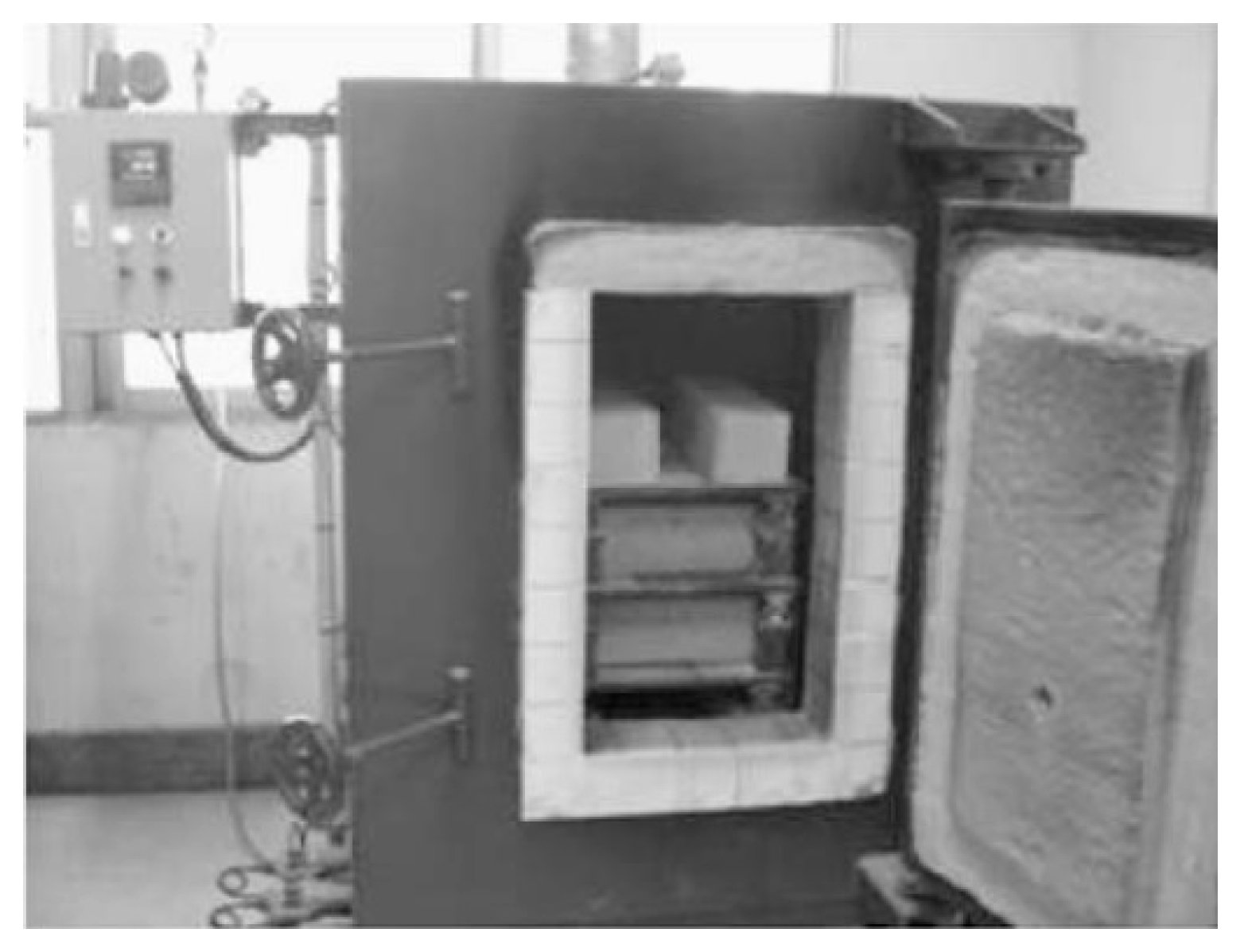
Figure 1.
Specimens in oven chamber according to ASTM E119-98.
Figure 1.
Specimens in oven chamber according to ASTM E119-98.
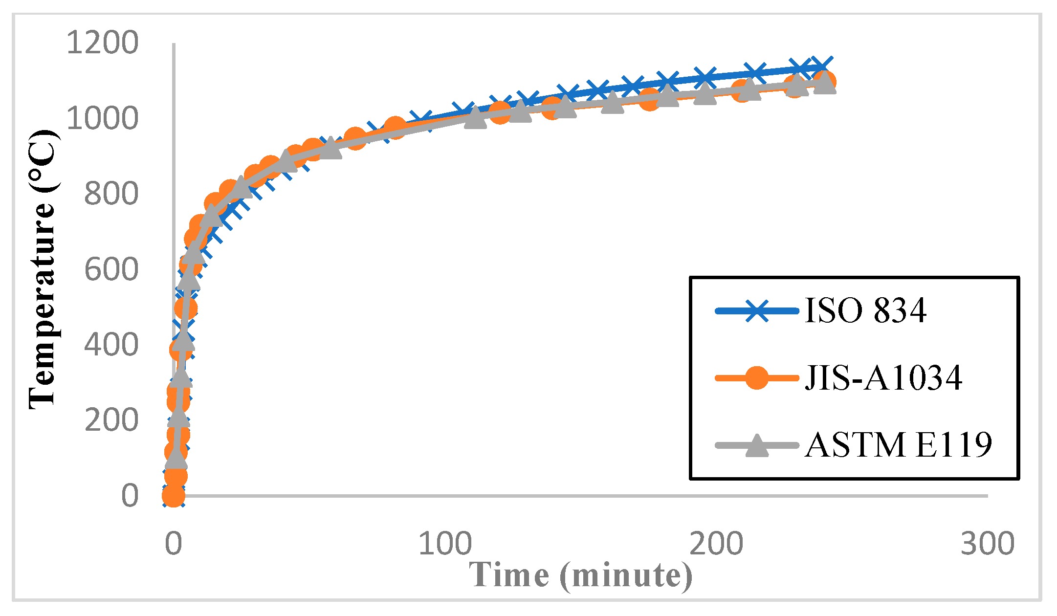
Figure 2.
Standard fire curves.
Figure 2.
Standard fire curves.
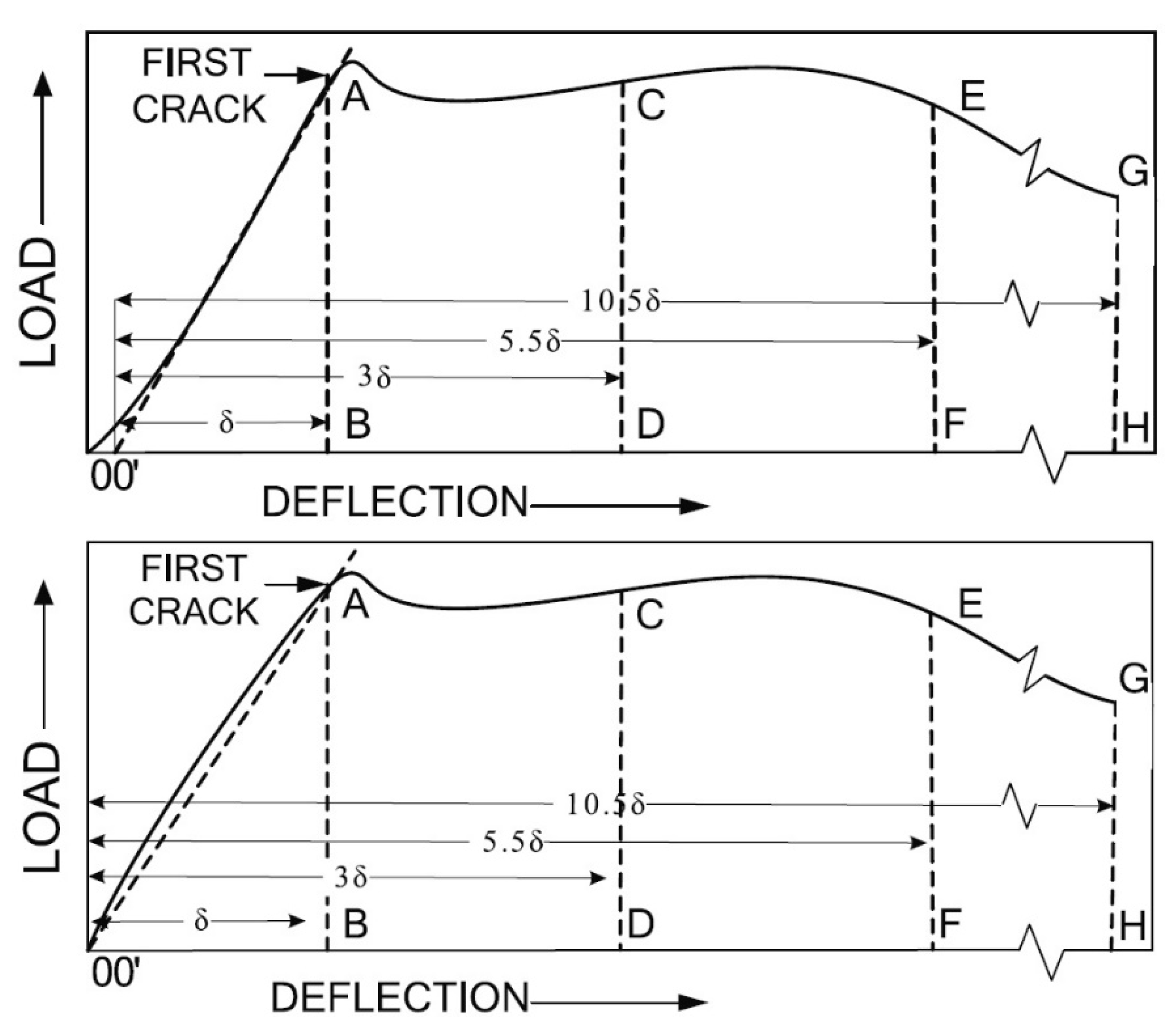
Figure 3.
Process of calculating toughness indexes (ASTM C1018).
Figure 3.
Process of calculating toughness indexes (ASTM C1018).
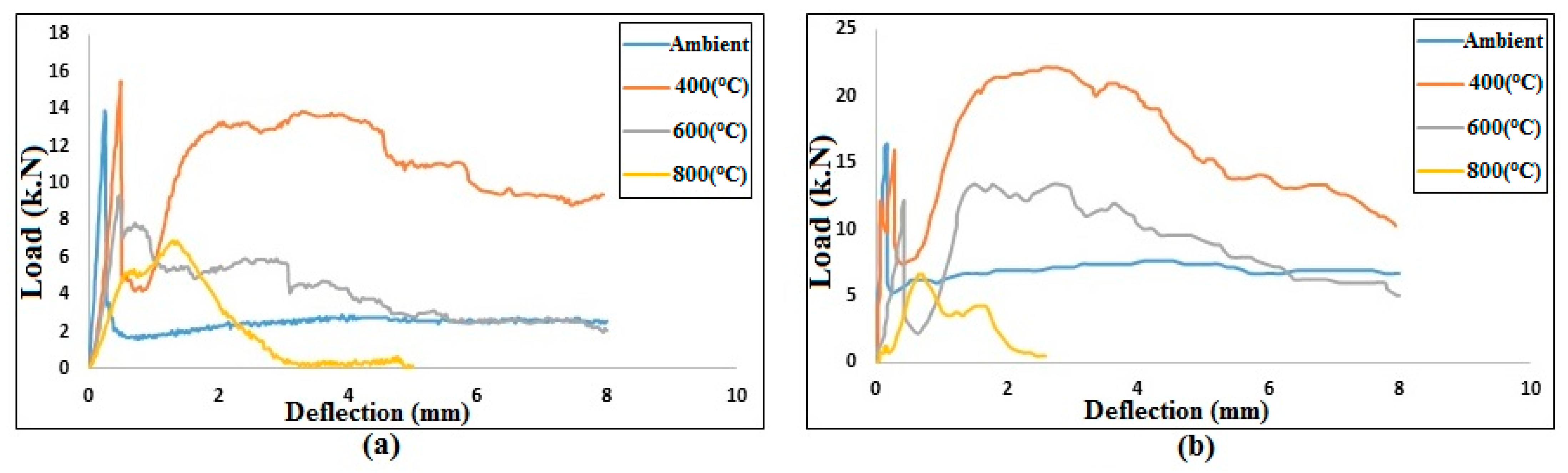
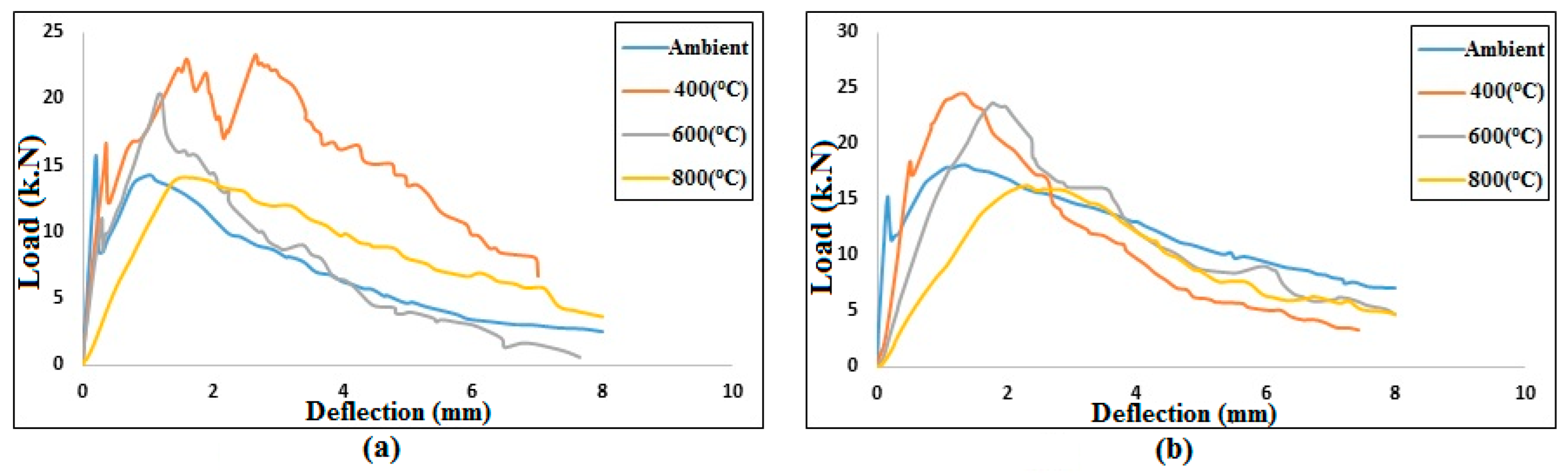
Figure 4.
Flexural responses of (a) 0.5% PEFRC and (b) 1.0% PEFRC after thermal expansion.
Figure 4.
Flexural responses of (a) 0.5% PEFRC and (b) 1.0% PEFRC after thermal expansion.
Figure 5.
Flexural responses of (a) 0.5% PPFRC and (b) 1.0% PPFRC after thermal expansion.
Figure 5.
Flexural responses of (a) 0.5% PPFRC and (b) 1.0% PPFRC after thermal expansion.
Figure 6.
Flexural responses of (a) 0.5% SFRC and (b) 1.0% SFRC after thermal expansion.
Figure 6.
Flexural responses of (a) 0.5% SFRC and (b) 1.0% SFRC after thermal expansion.
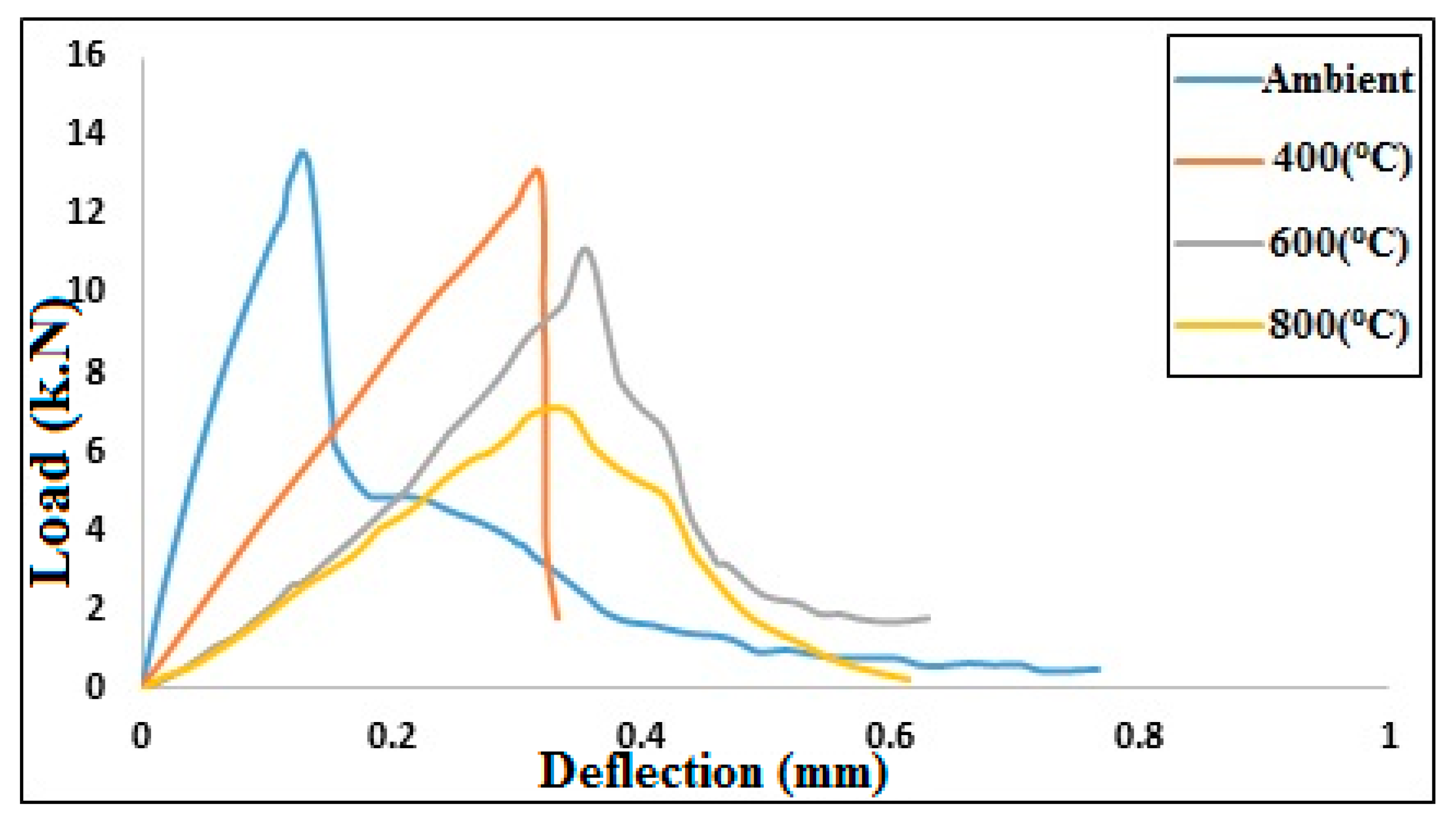
Figure 7.
Flexural response of plain concrete after thermal expansion.
Figure 7.
Flexural response of plain concrete after thermal expansion.
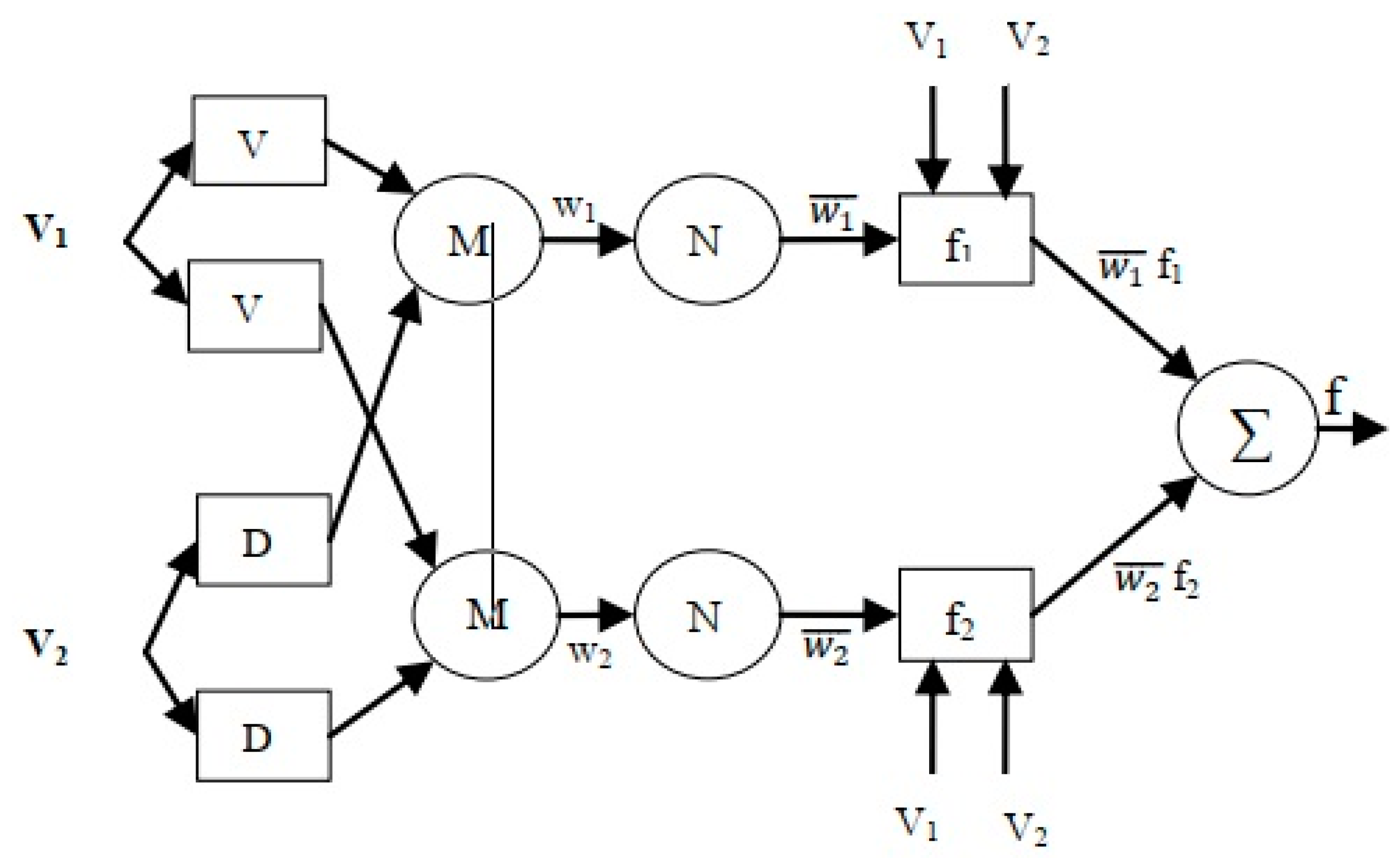
Figure 8.
Typical architecture of ANFIS [
2].
Figure 8.
Typical architecture of ANFIS [
2].
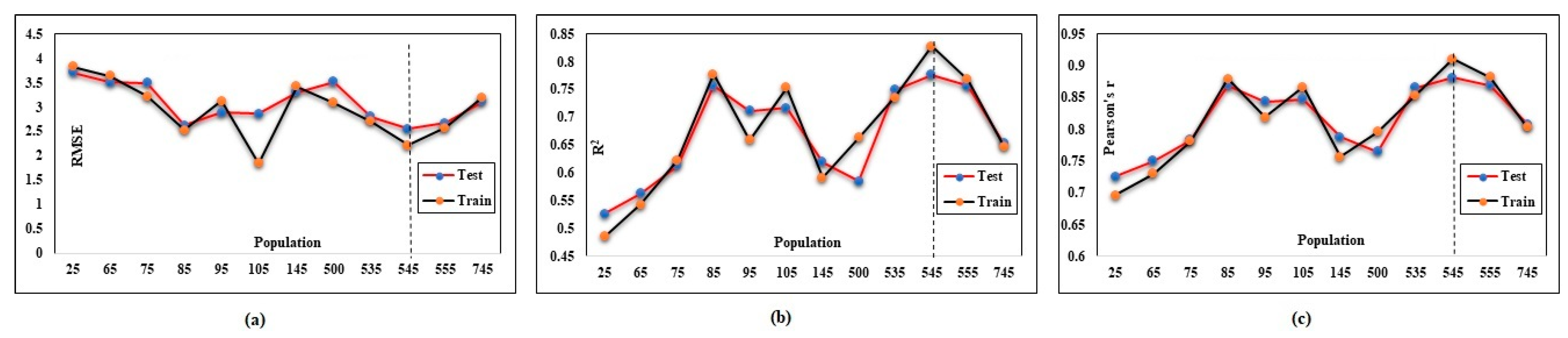
Figure 11.
ANFIS-PSO adjustment based on population number: (a) effect of population number on (RMSE), (b) effect of population number on (R2), (c) effect of population number on (r).
Figure 11.
ANFIS-PSO adjustment based on population number: (a) effect of population number on (RMSE), (b) effect of population number on (R2), (c) effect of population number on (r).
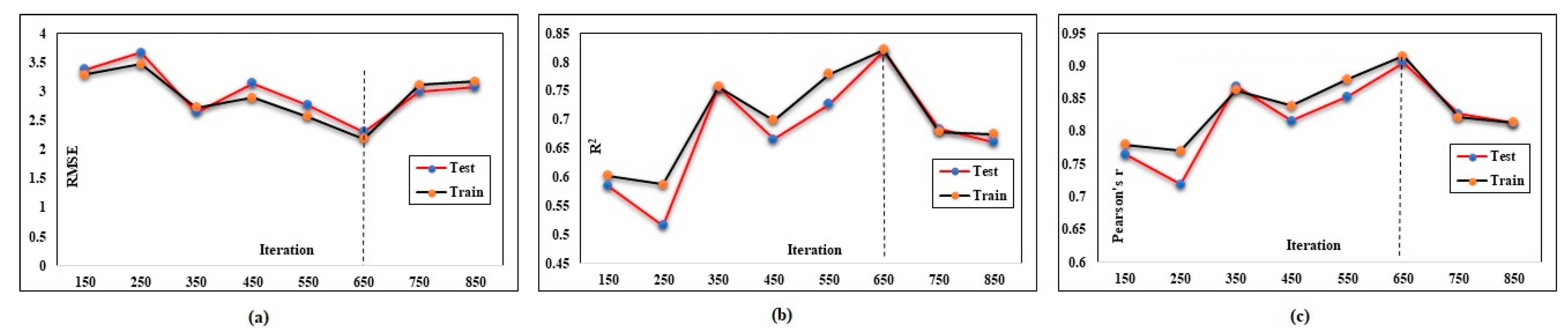
Figure 12.
ANFIS-PSO adjustment based on iteration number: (a) effect of iteration number on (RMSE), (b) effect of iteration number on (R2), (c) effect of iteration number on (r).
Figure 12.
ANFIS-PSO adjustment based on iteration number: (a) effect of iteration number on (RMSE), (b) effect of iteration number on (R2), (c) effect of iteration number on (r).
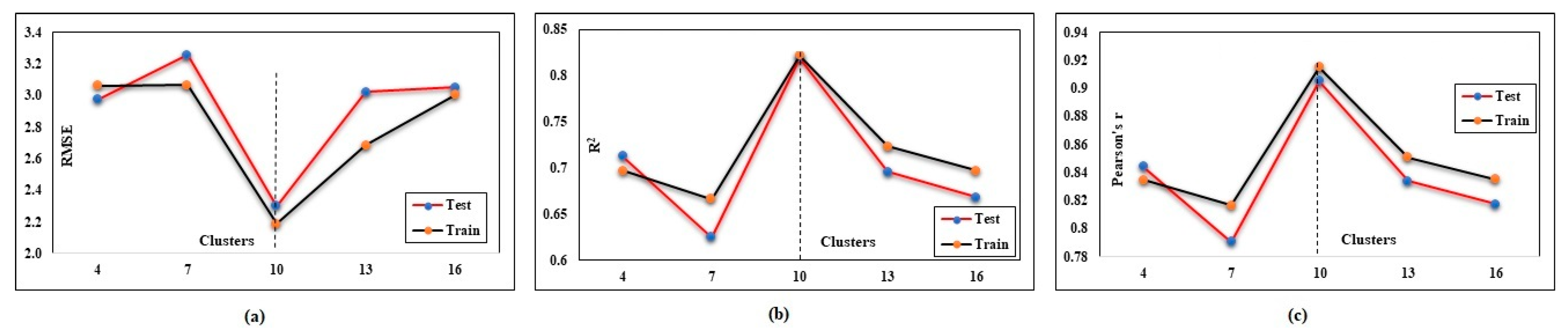
Figure 13.
ANFIS-PSO adjustment based on cluster number: (a) effect of cluster number on (RMSE), (b) effect of cluster number on (R2), (c) effect of cluster number on (r).
Figure 13.
ANFIS-PSO adjustment based on cluster number: (a) effect of cluster number on (RMSE), (b) effect of cluster number on (R2), (c) effect of cluster number on (r).
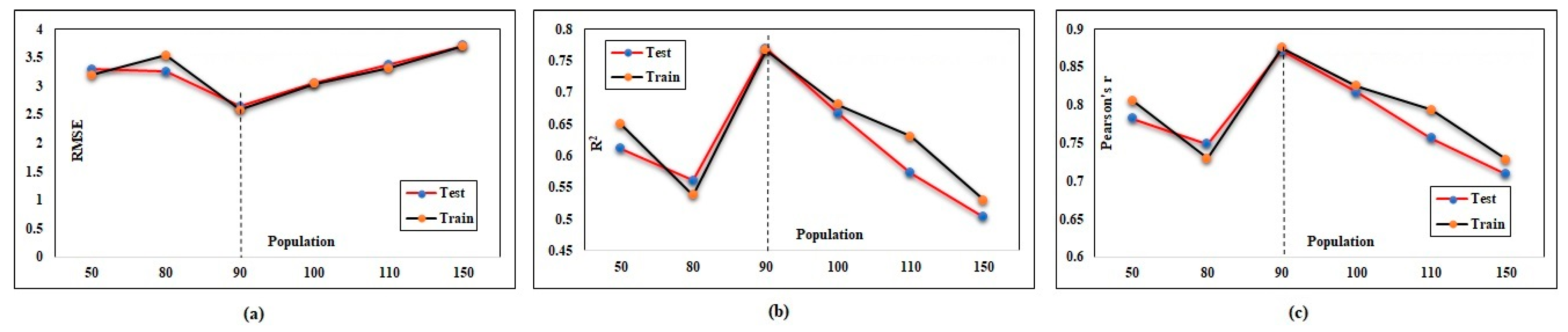
Figure 14.
APG adjustment based on population number: (a) effect of population number on (RMSE), (b) effect of population number on (R2), (c) effect of population number on (r).
Figure 14.
APG adjustment based on population number: (a) effect of population number on (RMSE), (b) effect of population number on (R2), (c) effect of population number on (r).
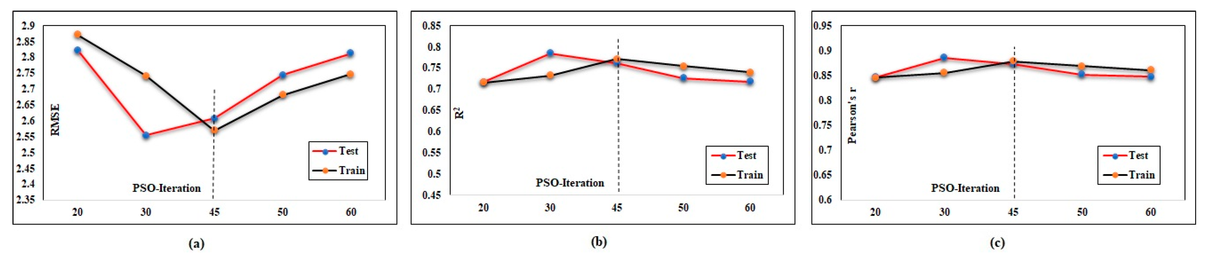
Figure 15.
APG adjustment based on PSO iteration number: (a) effect of iteration number on (RMSE), (b) effect of iteration number on (R2), (c) effect of iteration number on (r).
Figure 15.
APG adjustment based on PSO iteration number: (a) effect of iteration number on (RMSE), (b) effect of iteration number on (R2), (c) effect of iteration number on (r).
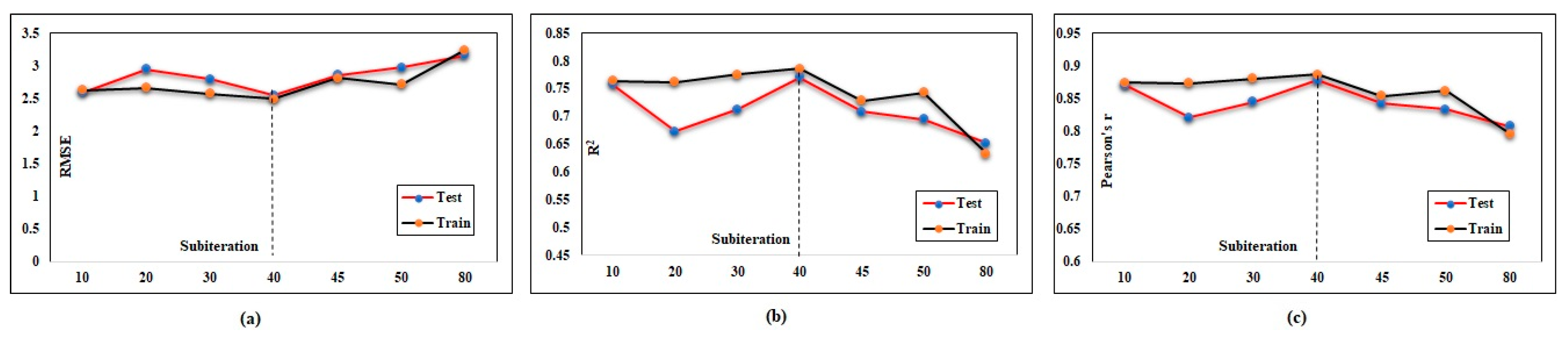
Figure 16.
APG adjustment based on GA sub-iteration number: (a) effect of sub-iteration number on (RMSE), (b) effect of sub-iteration number on (R2), (c) effect of sub-iteration number on (r).
Figure 16.
APG adjustment based on GA sub-iteration number: (a) effect of sub-iteration number on (RMSE), (b) effect of sub-iteration number on (R2), (c) effect of sub-iteration number on (r).
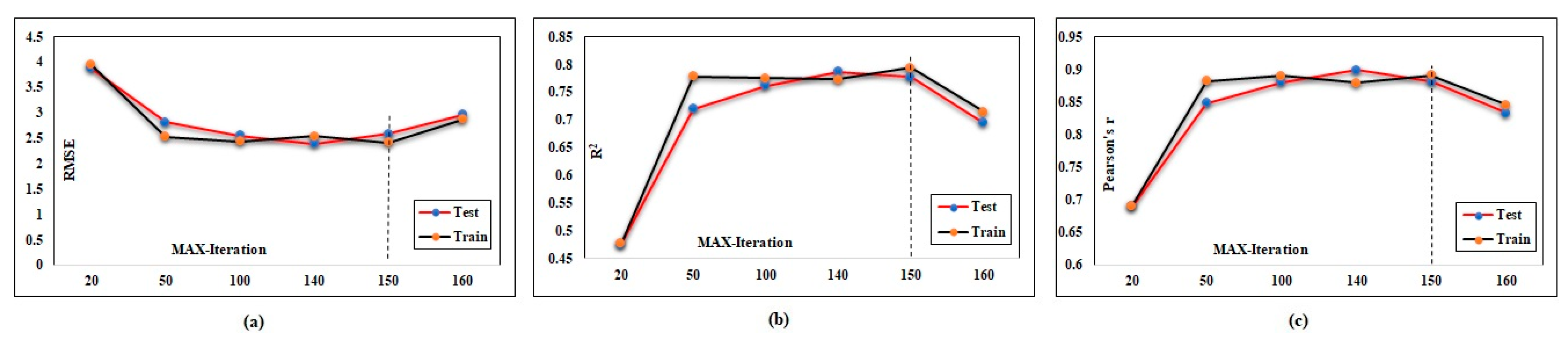
Figure 17.
APG adjustment based on MAX iteration number: (a) effect of MAX iteration number on (RMSE), (b) effect of MAX iteration number on (R2), (c) effect of MAX iteration number on (r).
Figure 17.
APG adjustment based on MAX iteration number: (a) effect of MAX iteration number on (RMSE), (b) effect of MAX iteration number on (R2), (c) effect of MAX iteration number on (r).
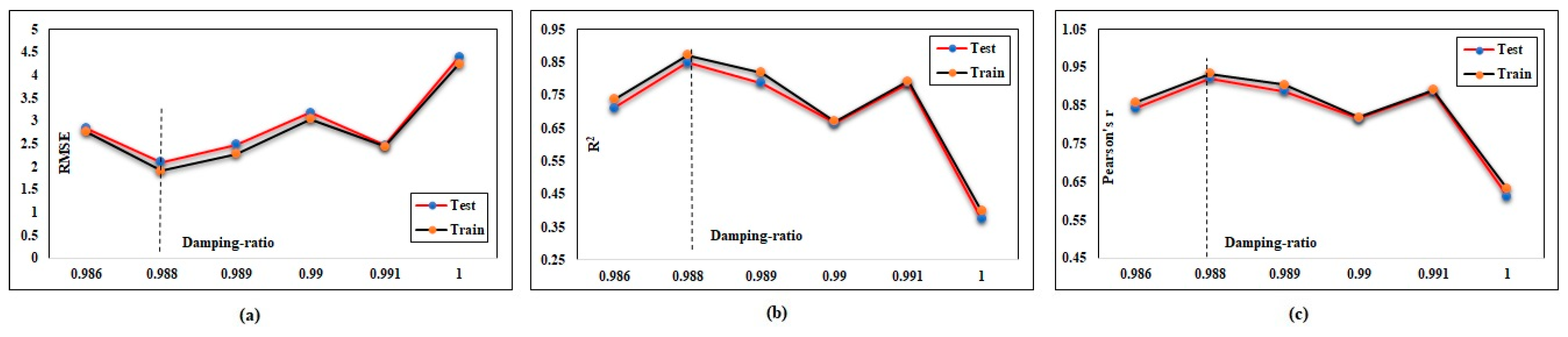
Figure 18.
APG adjustment based on damping ratio number: (a) effect of damping ratio number on (RMSE), (b) effect of damping ratio number on (R2), (c) effect of damping ratio number on (r).
Figure 18.
APG adjustment based on damping ratio number: (a) effect of damping ratio number on (RMSE), (b) effect of damping ratio number on (R2), (c) effect of damping ratio number on (r).
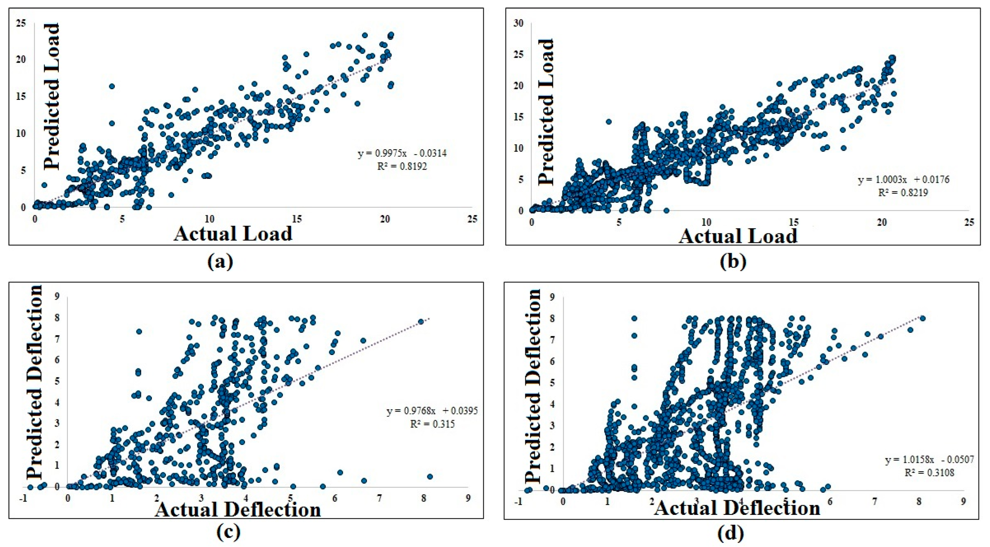
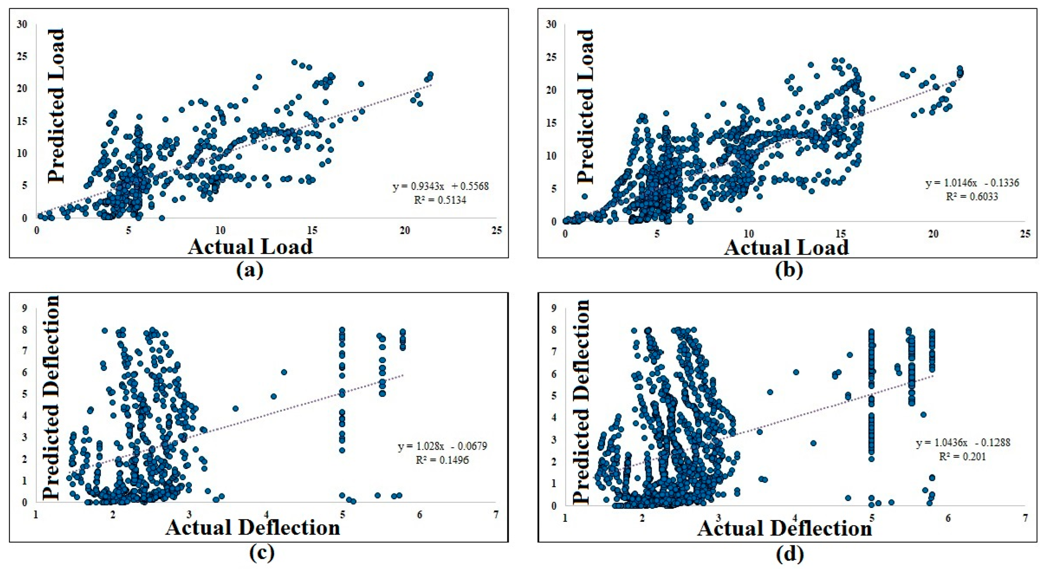
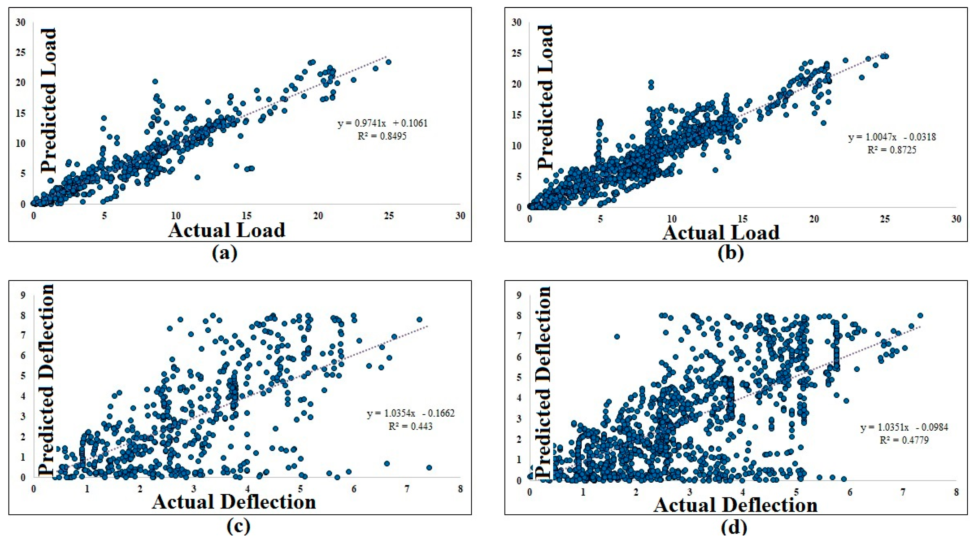
Figure 19.
ANFIS-PSO prediction vs. experimental results regression for subdatabase1: (a) flexural load test phase, (b) flexural load train phase, (c) deflection test phase, (d) deflection train phase.
Figure 19.
ANFIS-PSO prediction vs. experimental results regression for subdatabase1: (a) flexural load test phase, (b) flexural load train phase, (c) deflection test phase, (d) deflection train phase.
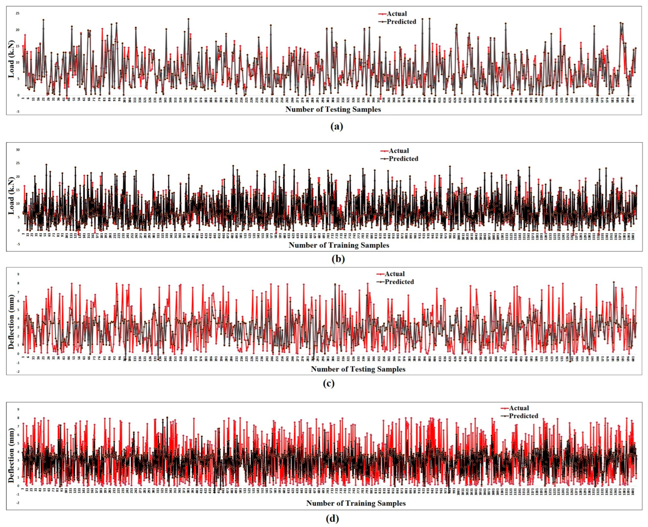
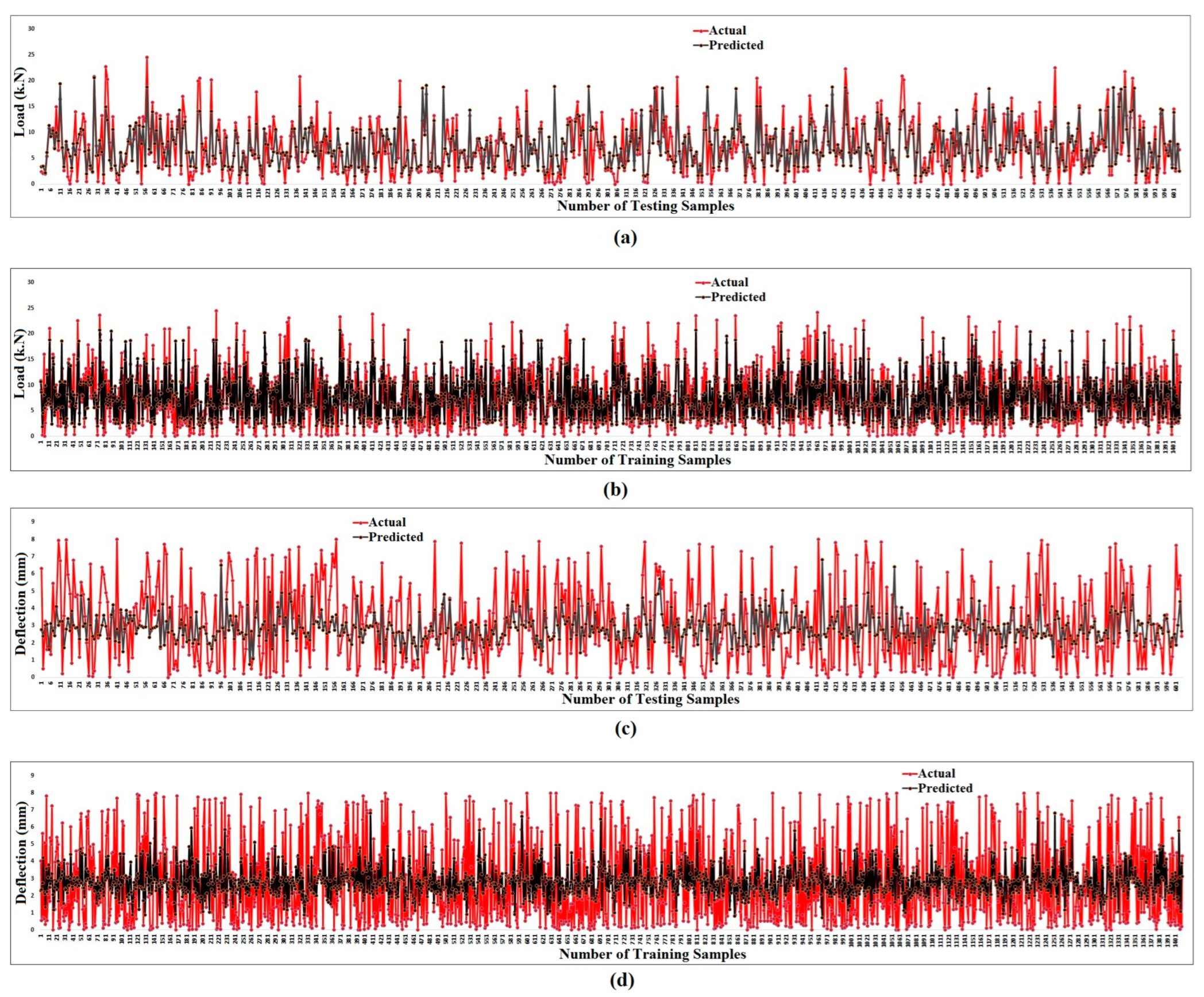
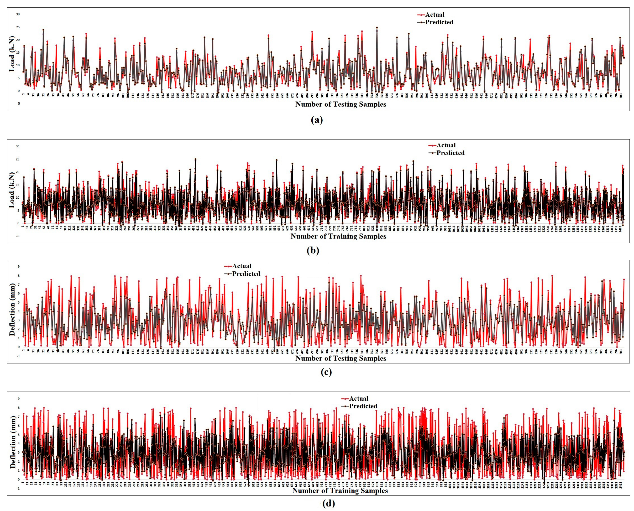
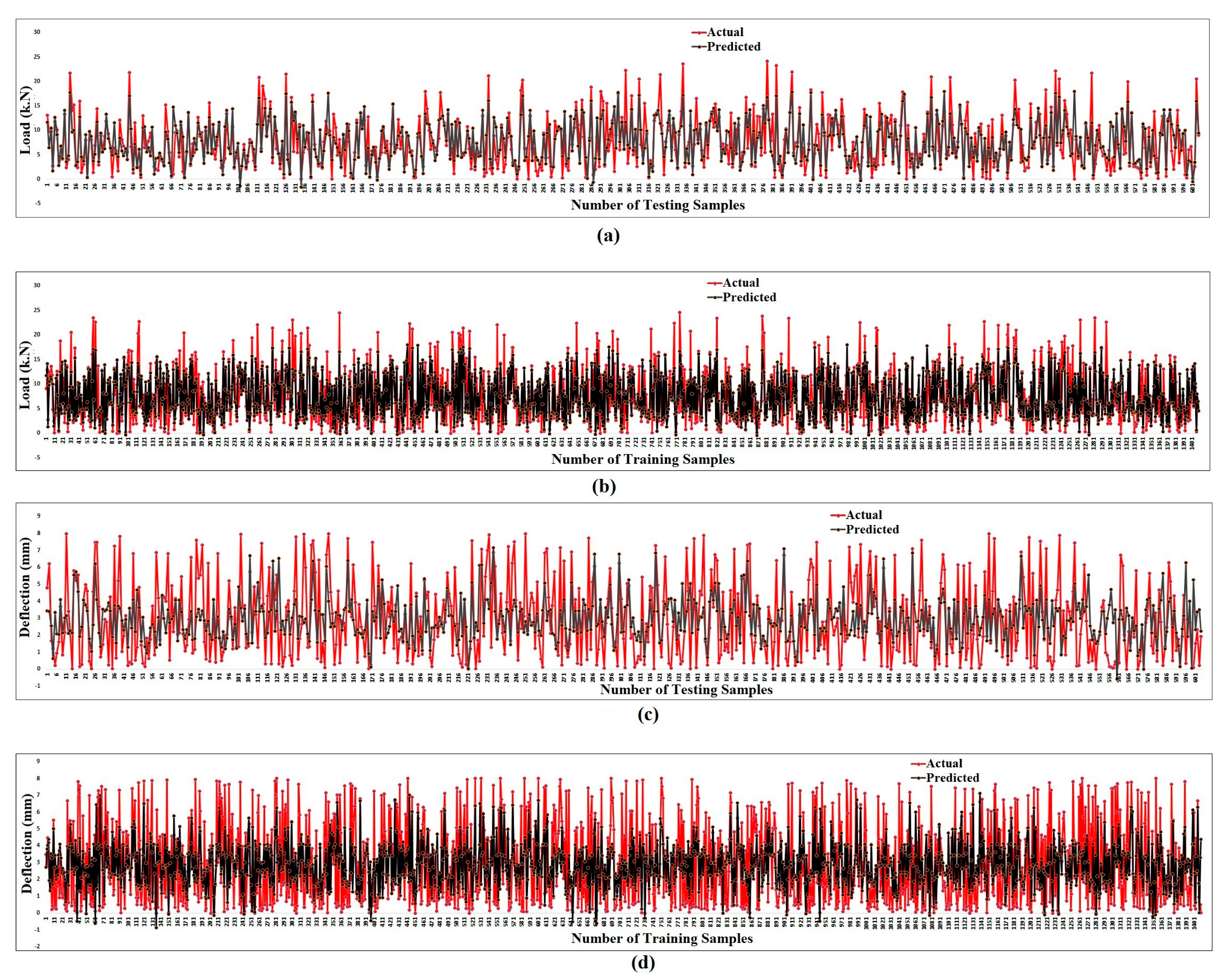
Figure 20.
ANFIS-PSO prediction vs. experimental diagram for subdatabase1: (a) flexural load test phase, (b) flexural load train phase, (c) deflection test phase, (d) deflection train phase.
Figure 20.
ANFIS-PSO prediction vs. experimental diagram for subdatabase1: (a) flexural load test phase, (b) flexural load train phase, (c) deflection test phase, (d) deflection train phase.
Figure 21.
ANFIS-PSO prediction vs. experimental results regression for subdatabase2: (a) flexural load test phase, (b) flexural load train phase, (c) deflection test phase, (d) deflection train phase.
Figure 21.
ANFIS-PSO prediction vs. experimental results regression for subdatabase2: (a) flexural load test phase, (b) flexural load train phase, (c) deflection test phase, (d) deflection train phase.
Figure 22.
ANFIS-PSO prediction vs. experimental diagram for subdatabase2: (a) flexural load test phase, (b) flexural load train phase, (c) deflection test phase, (d) deflection train phase.
Figure 22.
ANFIS-PSO prediction vs. experimental diagram for subdatabase2: (a) flexural load test phase, (b) flexural load train phase, (c) deflection test phase, (d) deflection train phase.
Figure 23.
ANFIS-PSO prediction vs. experimental results regression for subdatabase3: (a) flexural load test phase, (b) flexural load train phase, (c) deflection test phase, (d) deflection train phase.
Figure 23.
ANFIS-PSO prediction vs. experimental results regression for subdatabase3: (a) flexural load test phase, (b) flexural load train phase, (c) deflection test phase, (d) deflection train phase.
Figure 24.
ANFIS-PSO prediction vs. experimental diagram for subdatabase3: (a) flexural load test phase, (b) flexural load train phase, (c) deflection test phase, (d) deflection train phase.
Figure 24.
ANFIS-PSO prediction vs. experimental diagram for subdatabase3: (a) flexural load test phase, (b) flexural load train phase, (c) deflection test phase, (d) deflection train phase.
Figure 25.
ANFIS-PSO prediction vs. experimental results regression for subdatabase4: (a) flexural toughness test phase, (b) flexural toughness train phase.
Figure 25.
ANFIS-PSO prediction vs. experimental results regression for subdatabase4: (a) flexural toughness test phase, (b) flexural toughness train phase.
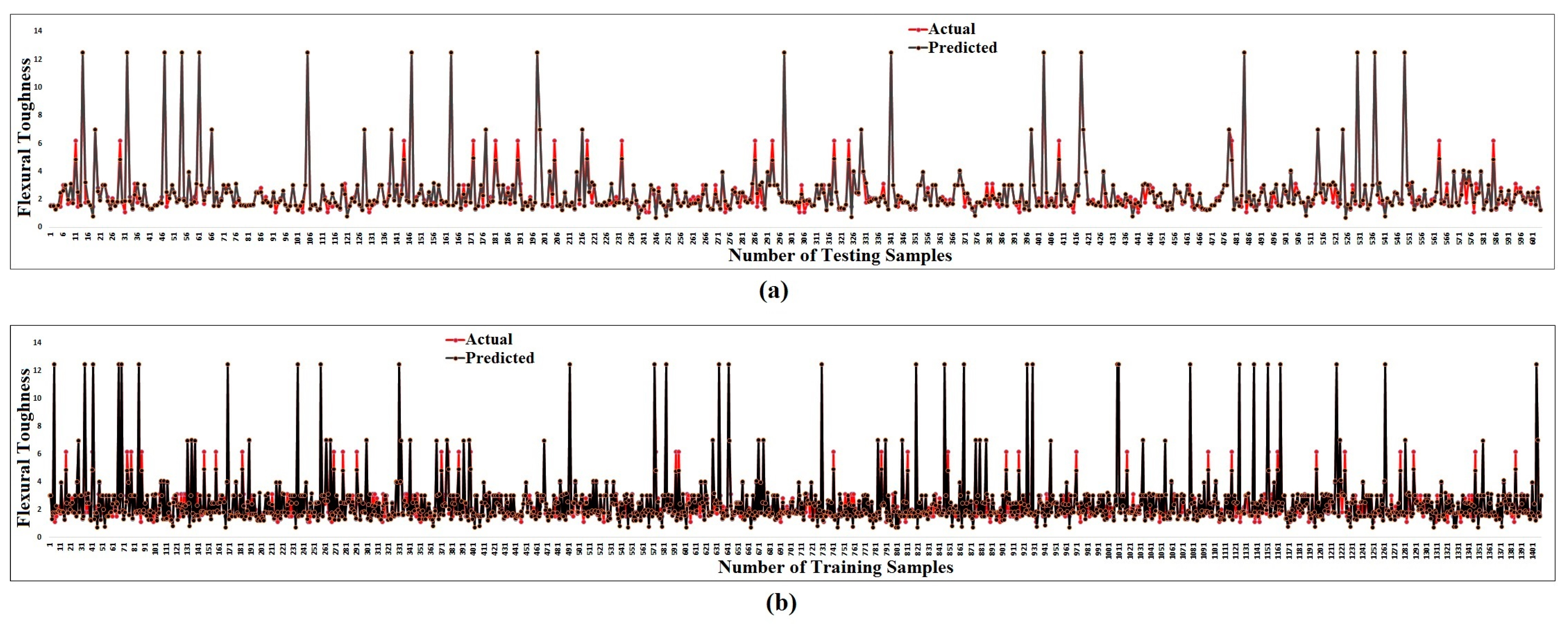
Figure 26.
ANFIS-PSO prediction vs. experimental diagram for subdatabase4: (a) flexural load toughness phase, (b) flexural toughness train phase.
Figure 26.
ANFIS-PSO prediction vs. experimental diagram for subdatabase4: (a) flexural load toughness phase, (b) flexural toughness train phase.
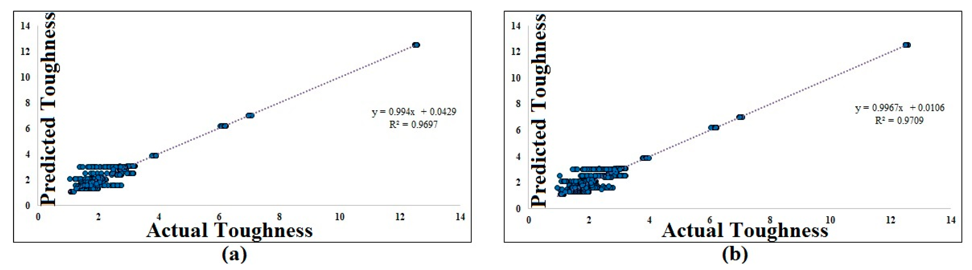
Figure 27.
ANFIS-PSO prediction vs. experimental results regression for subdatabase5: (a) flexural toughness test phase, (b) flexural toughness train phase.
Figure 27.
ANFIS-PSO prediction vs. experimental results regression for subdatabase5: (a) flexural toughness test phase, (b) flexural toughness train phase.
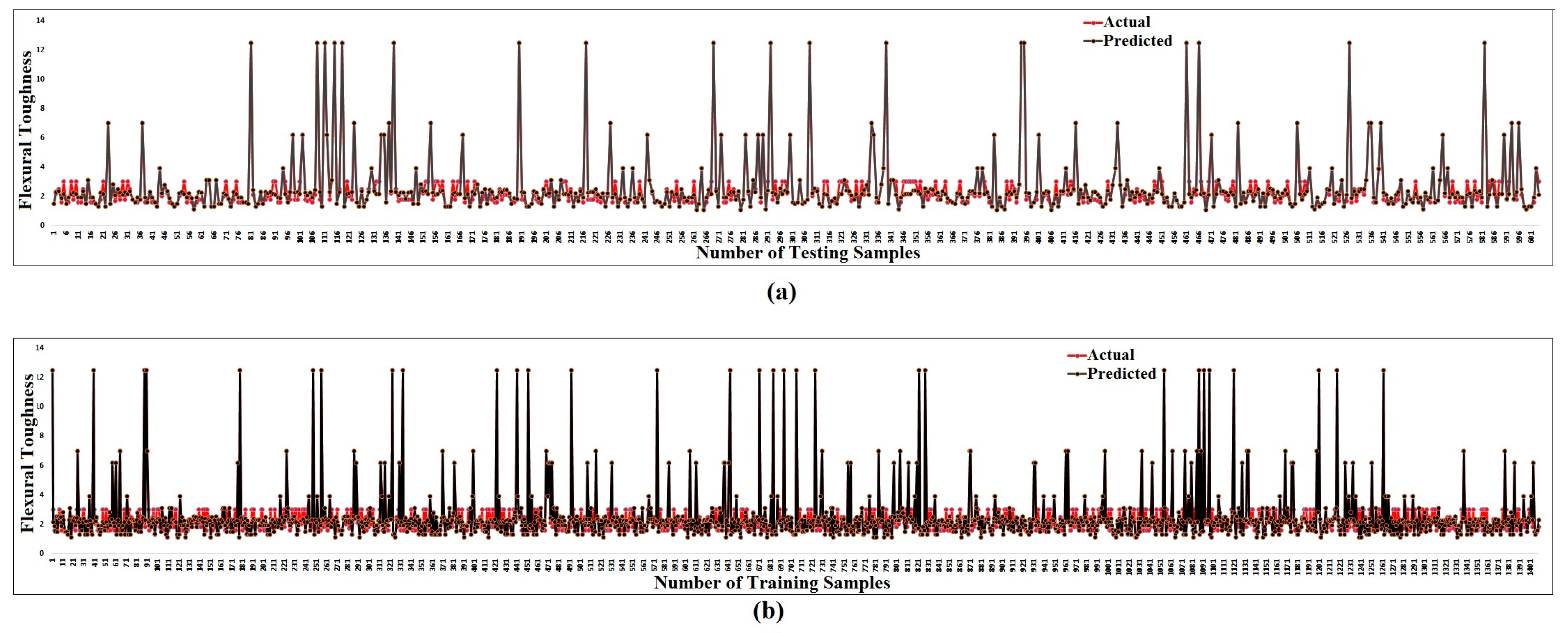
Figure 28.
ANFIS-PSO prediction vs. experimental diagram for subdatabase5: (a) flexural load toughness phase, (b) flexural toughness train phase.
Figure 28.
ANFIS-PSO prediction vs. experimental diagram for subdatabase5: (a) flexural load toughness phase, (b) flexural toughness train phase.
Figure 29.
APG prediction vs. experimental results regression for subdatabase1: (a) flexural load test phase, (b) flexural load train phase, (c) deflection test phase, (d) deflection train phase.
Figure 29.
APG prediction vs. experimental results regression for subdatabase1: (a) flexural load test phase, (b) flexural load train phase, (c) deflection test phase, (d) deflection train phase.
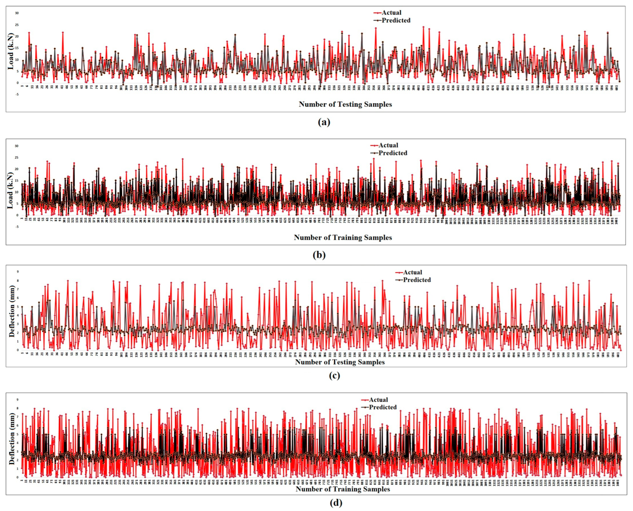
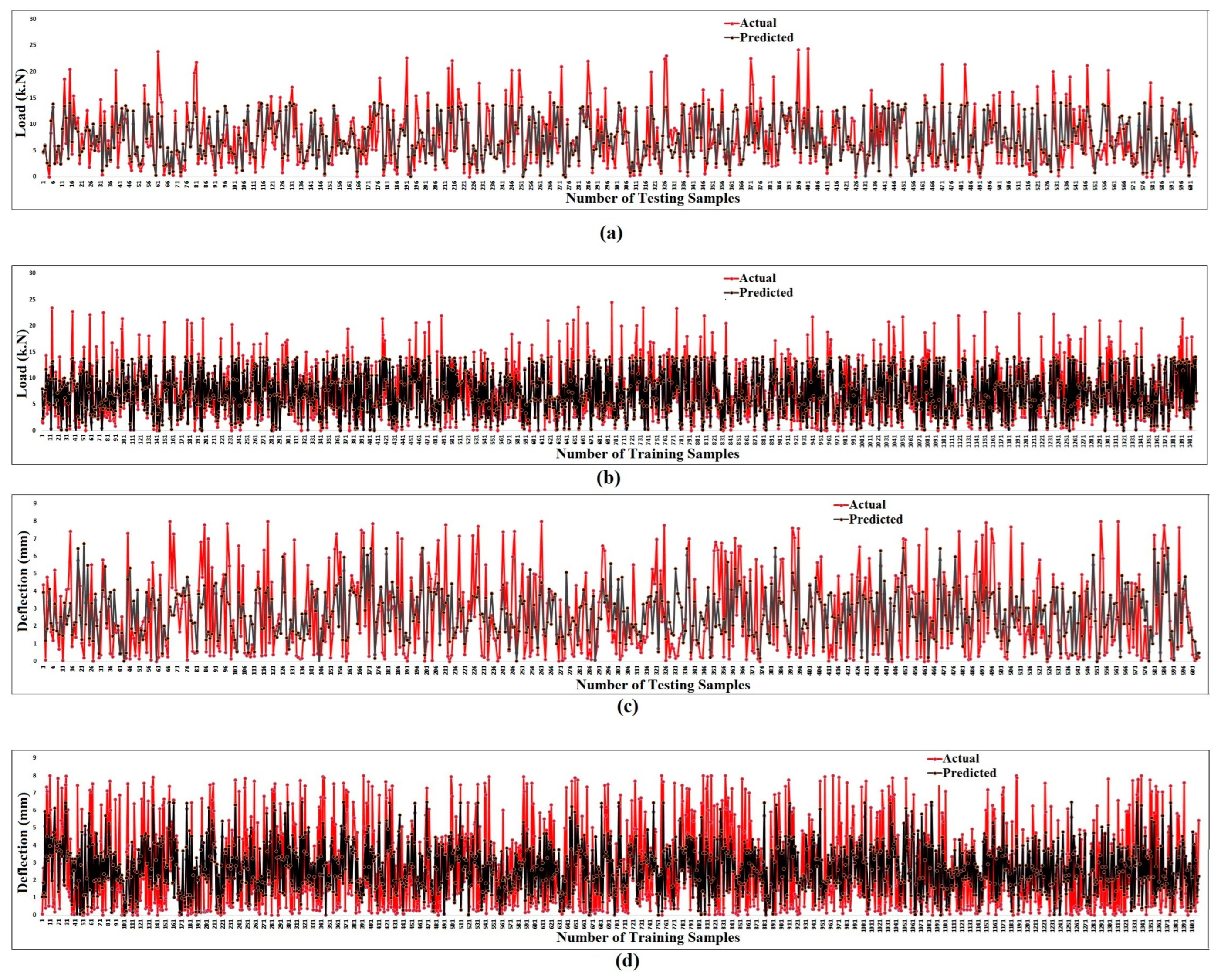
Figure 30.
APG prediction vs. experimental diagram for subdatabase1: (a) flexural load test phase, (b) flexural load train phase, (c) deflection test phase, (d) deflection train phase.
Figure 30.
APG prediction vs. experimental diagram for subdatabase1: (a) flexural load test phase, (b) flexural load train phase, (c) deflection test phase, (d) deflection train phase.
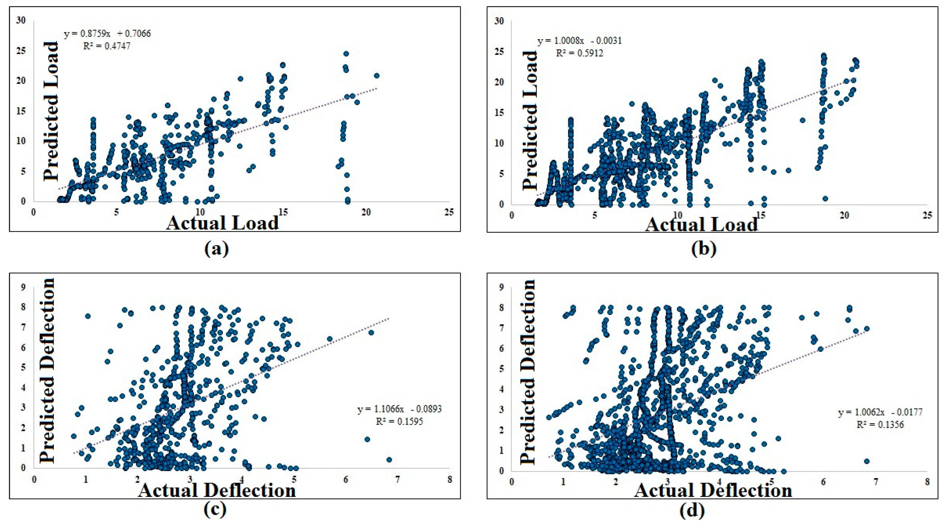
Figure 31.
APG prediction vs. experimental results regression for subdatabase2: (a) flexural load test phase, (b) flexural load train phase, (c) deflection test phase, (d) deflection train phase.
Figure 31.
APG prediction vs. experimental results regression for subdatabase2: (a) flexural load test phase, (b) flexural load train phase, (c) deflection test phase, (d) deflection train phase.
Figure 32.
APG prediction vs. experimental diagram for subdatabase2: (a) flexural load test phase, (b) flexural load train phase, (c) deflection test phase, (d) deflection train phase.
Figure 32.
APG prediction vs. experimental diagram for subdatabase2: (a) flexural load test phase, (b) flexural load train phase, (c) deflection test phase, (d) deflection train phase.
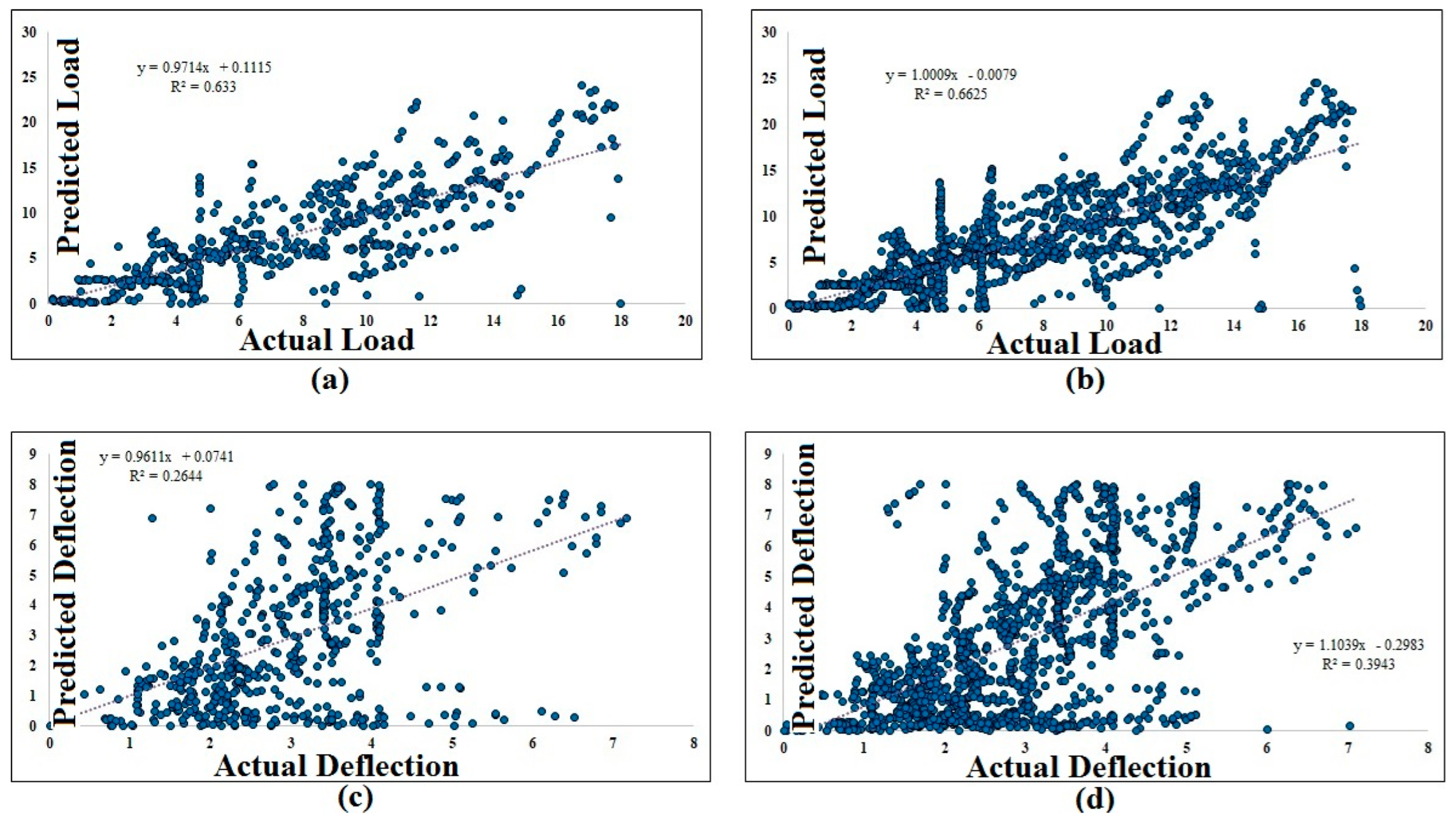
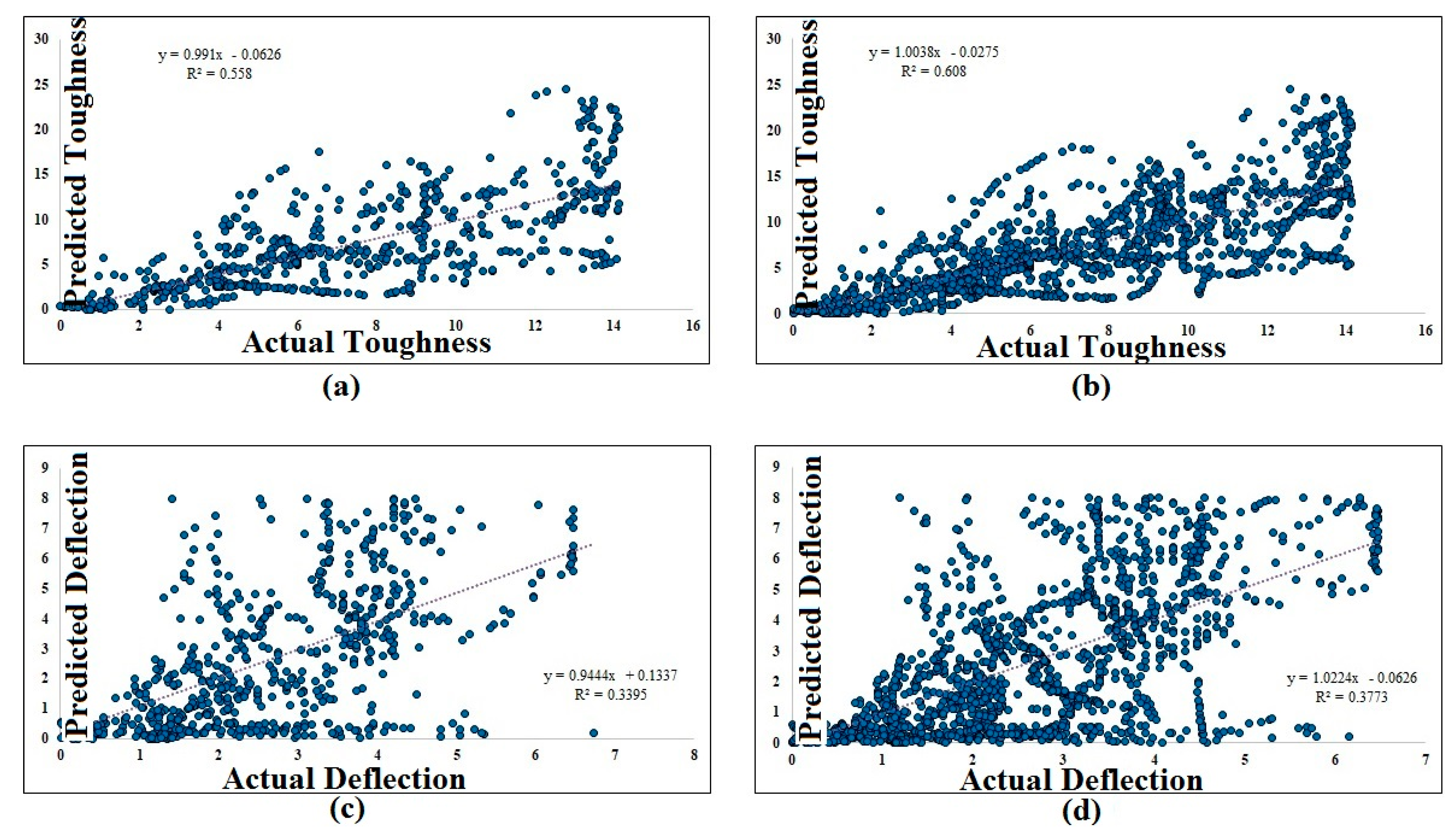
Figure 33.
APG prediction vs. experimental results regression for subdatabase3: (a) flexural load test phase, (b) flexural load train phase, (c) deflection test phase, (d) deflection train phase.
Figure 33.
APG prediction vs. experimental results regression for subdatabase3: (a) flexural load test phase, (b) flexural load train phase, (c) deflection test phase, (d) deflection train phase.
Figure 34.
APG prediction vs. experimental diagram for subdatabase3: (a) flexural load test phase, (b) flexural load train phase, (c) deflection test phase, (d) deflection train phase.
Figure 34.
APG prediction vs. experimental diagram for subdatabase3: (a) flexural load test phase, (b) flexural load train phase, (c) deflection test phase, (d) deflection train phase.
Figure 35.
APG prediction vs. experimental results regression for subdatabase4: (a) flexural toughness test phase, (b) flexural toughness train phase.
Figure 35.
APG prediction vs. experimental results regression for subdatabase4: (a) flexural toughness test phase, (b) flexural toughness train phase.
Figure 36.
APG prediction vs. experimental diagram for subdatabase4: (a) flexural load toughness phase, (b) flexural toughness train phase.
Figure 36.
APG prediction vs. experimental diagram for subdatabase4: (a) flexural load toughness phase, (b) flexural toughness train phase.
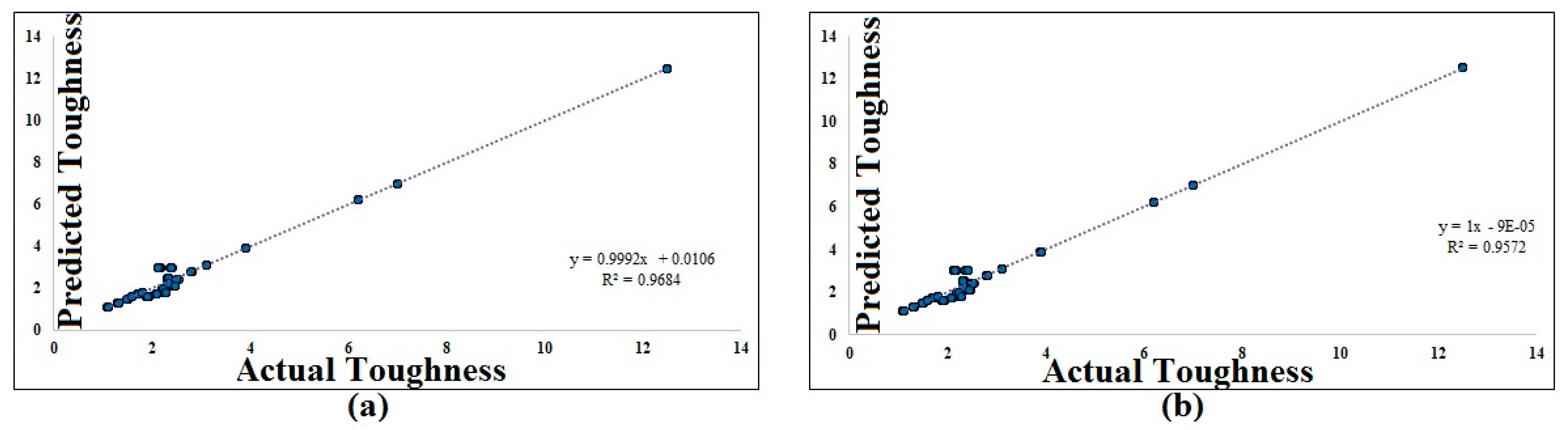
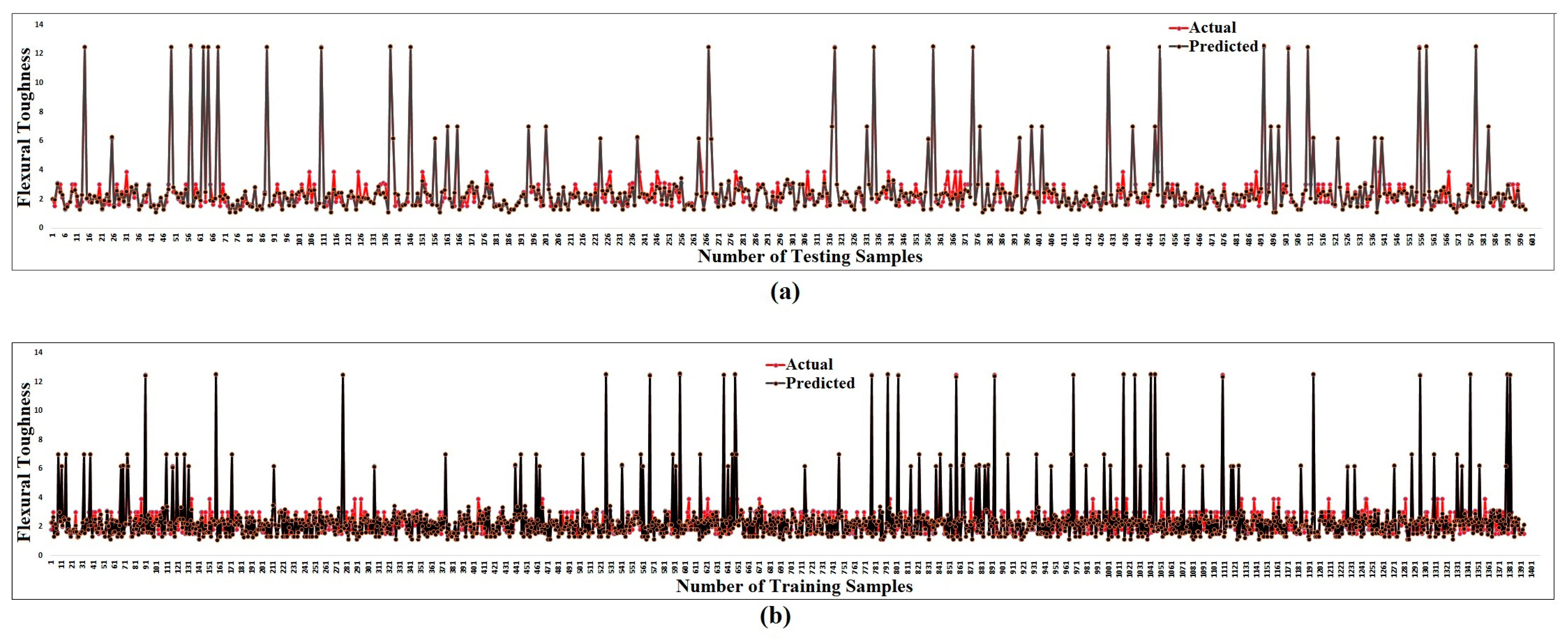
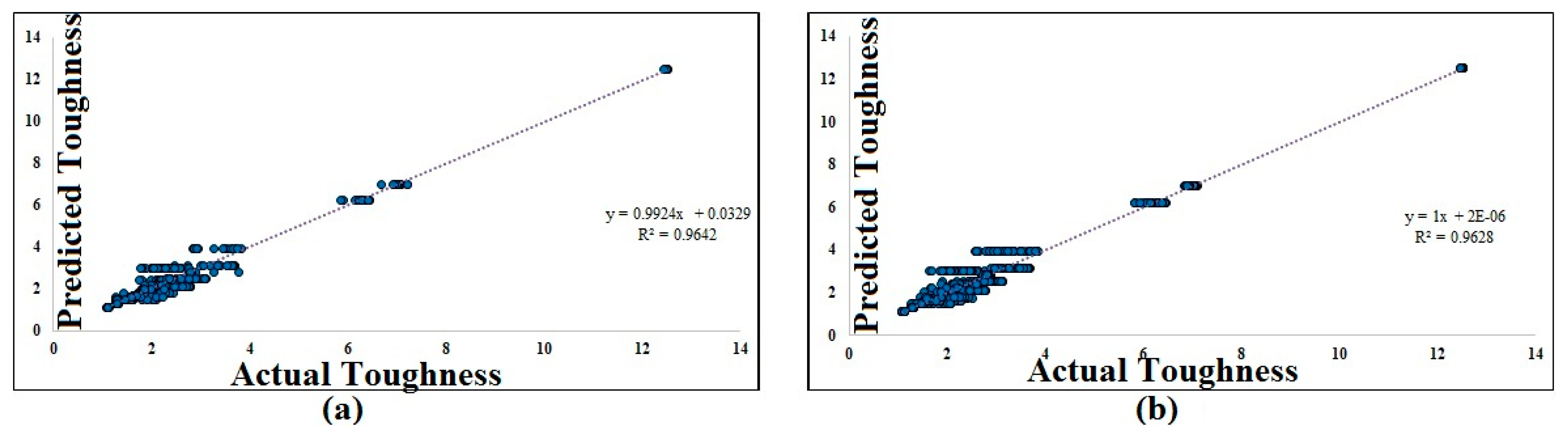
Figure 37.
APG prediction vs. experimental results regression for subdatabase5: (a) flexural toughness test phase, (b) flexural toughness train phase.
Figure 37.
APG prediction vs. experimental results regression for subdatabase5: (a) flexural toughness test phase, (b) flexural toughness train phase.
Figure 38.
APG prediction vs. experimental diagram for subdatabase5: (a) flexural load toughness phase, (b) flexural toughness train phase.
Figure 38.
APG prediction vs. experimental diagram for subdatabase5: (a) flexural load toughness phase, (b) flexural toughness train phase.
Table 1.
Typical fiber features.
Table 1.
Typical fiber features.
| Fiber Type | Specific Gravity (kg/m3) | Modulus of Elasticity (Gpa) | Tensile Strength (Mpa) | Elongation at Break (%) | Acid/Alkali Resistance | Cost ($/kg) |
|---|
| Polypropylene (PP) [14,15,16] | 910 | 1.5–12 | 240–900 | 15–80 | High | 1–2.5 |
| Polyethylene (PE) [17,18,19] | 920–960 | 5–100 | 80–600 | 4–100 | High | 2–20 |
| Steel (ST) for comparison [20] | 7840 | 200 | 500–2000 | 0.5–3.5 | Low to High | 1–8 |
Table 2.
Details of the input and output variables.
Table 2.
Details of the input and output variables.
| Inputs and Outputs | Variables | Minimum | Maximum | Mean Value | Standard Deviation |
|---|
| Input 1 | Temperature (°C) | 25.00 | 800.00 | 456.25 | 272.92 |
| Input 2 | Fiber content (%) | 0.00 | 1.00 | 0.50 | 0.23 |
| Input 3 | Tensile strength of fiber (N./mm2) | 450.00 | 1000.00 | 690.00 | 188.85 |
| Input 4 | Aspect ratio of fiber (l/d) | 52.00 | 90.00 | 68.67 | 16.29 |
| Input 5 | Toughness index | 1.80 | 6.80 | 3.91 | 1.42 |
| Input 6 | Flexural toughness | 1.10 | 12.50 | 2.54 | 1.95 |
| Input 7 | Pulse velocity | 2808 | 4795 | 4033.27 | 640.17 |
| Input 8 | Deflection (mm) | 0.00 | 8.00 | 2.68 | 2.35 |
| Input 9 | Load (k.N) | 0.00 | 24.54 | 7.29 | 5.29 |
| Output 1 | Load (k.N) | 0.00 | 24.54 | 7.29 | 5.29 |
| Output 2 | Deflection (mm) | 0.00 | 8.00 | 2.68 | 2.35 |
| Output 3 | Flexural toughness | 1.10 | 12.50 | 2.54 | 1.95 |
Table 3.
Inputs and outputs of subdatabase1.
Table 3.
Inputs and outputs of subdatabase1.
| Inputs and Outputs | Minimum | Maximum | Average |
|---|
| Temperature (°C) | 25.00 | 800.00 | 456.25 |
| 1.10 | 12.50 | 2.54 |
| 1.80 | 6.80 | 3.91 |
| Deflection (mm) * | 0.00 | 8.00 | 2.68 |
| Load (kN) * | 0.00 | 24.54 | 7.29 |
Table 4.
Inputs and outputs of subdatabase2.
Table 4.
Inputs and outputs of subdatabase2.
| Inputs and Outputs | Minimum | Maximum | Average |
|---|
| Temperature (°C) | 25.00 | 800.00 | 456.25 |
| Fiber content (%) | 0.00 | 1.00 | 0.50 |
| Tensile strength of fiber (N/mm2) | 450.00 | 1000.00 | 690.00 |
| Aspect ratio of fiber (l/d) | 52.00 | 90.00 | 68.67 |
| Deflection (mm) * | 0.00 | 8.00 | 2.68 |
| Load (kN) * | 0.00 | 24.54 | 7.29 |
Table 5.
Inputs and outputs of subdatabase3.
Table 5.
Inputs and outputs of subdatabase3.
| Inputs and Outputs | Minimum | Maximum | Average |
|---|
| Temperature (°C) | 25.00 | 800.00 | 456.25 |
| 2808 | 4795 | 4033.27 |
| Deflection (mm) * | 0.00 | 8.00 | 2.68 |
| Load (kN) * | 0.00 | 24.54 | 7.29 |
Table 6.
Inputs and outputs of subdatabase4.
Table 6.
Inputs and outputs of subdatabase4.
| Inputs and Outputs | Minimum | Maximum | Average |
|---|
| Temperature (°C) | 25.00 | 800.00 | 456.25 |
| Fiber content (%) | 0.00 | 1.00 | 0.50 |
| Tensile strength of fiber (N/mm2) | 450.00 | 1000.00 | 690.00 |
| Deflection (mm) * | 0.00 | 8.00 | 2.68 |
| * | 1.10 | 12.50 | 2.54 |
Table 7.
Inputs and outputs of subdatabase5.
Table 7.
Inputs and outputs of subdatabase5.
| Inputs and Outputs | Minimum | Maximum | Average |
|---|
| Temperature (°C) | 25.00 | 800.00 | 456.25 |
| Fiber content (%) | 0.00 | 1.00 | 0.50 |
| Tensile strength of fiber (N/mm2) | 450.00 | 1000.00 | 690.00 |
| Load (kN) | 0.00 | 24.54 | 7.29 |
| Deflection (mm) * | 0.00 | 8.00 | 2.68 |
| * | 1.10 | 12.50 | 2.54 |
Table 8.
Performance parameters of ANFIS-PSO adjustment based on population number.
Table 8.
Performance parameters of ANFIS-PSO adjustment based on population number.
| Population | Test | Train |
|---|
| RMSE | r | R2 | RMSE | r | R2 |
|---|
| 25 | 3.712577 | 0.725924 | 0.527 | 3.831084 | 0.696089 | 0.4859 |
| 65 | 3.508492 | 0.750727 | 0.5636 | 3.637986 | 0.729853 | 0.5429 |
| 75 | 3.497266 | 0.783102 | 0.6132 | 3.219799 | 0.781098 | 0.6227 |
| 85 | 2.626729 | 0.869537 | 0.7561 | 2.533611 | 0.879021 | 0.7777 |
| 95 | 2.885258 | 0.843709 | 0.7118 | 3.128901 | 0.818919 | 0.6597 |
| 105 | 2.865556 | 0.846867 | 0.7172 | 1.85006 | 0.866333 | 0.7532 |
| 145 | 3.30335 | 0.78746 | 0.6201 | 3.423689 | 0.756888 | 0.5915 |
| 500 | 3.513862 | 0.764782 | 0.5849 | 3.083961 | 0.796095 | 0.6635 |
| 535 | 2.803131 | 0.865807 | 0.7496 | 2.70398 | 0.853733 | 0.7355 |
| 545 | 2.55558 | 0.880936 | 0.776 | 2.223289 | 0.910195 | 0.828 |
| 555 | 2.669889 | 0.869614 | 0.7562 | 2.577172 | 0.881952 | 0.7678 |
| 745 | 3.110781 | 0.808255 | 0.6533 | 3.199169 | 0.803118 | 0.6475 |
Table 9.
Performance parameters of ANFIS-PSO adjustment based on iteration number.
Table 9.
Performance parameters of ANFIS-PSO adjustment based on iteration number.
| Iteration | Test | Train |
|---|
| RMSE | r | R2 | RMSE | r | R2 |
|---|
| 150 | 3.383412 | 0.764805 | 0.5849 | 3.292399 | 0.780195 | 0.6032 |
| 250 | 3.668915 | 0.718894 | 0.5168 | 3.463981 | 0.770327 | 0.5882 |
| 350 | 2.6410 | 0.869586 | 0.7562 | 2.7200 | 0.86274 | 0.7574 |
| 450 | 3.1374 | 0.81602 | 0.6659 | 2.8910 | 0.839018 | 0.6994 |
| 550 | 2.7653 | 0.852937 | 0.7275 | 2.5608 | 0.879944 | 0.7792 |
| 650 | 2.3018 | 0.905074 | 0.8192 | 2.1895 | 0.914906 | 0.8219 |
| 750 | 3.003843 | 0.826912 | 0.6838 | 3.1114 | 0.821586 | 0.6793 |
| 850 | 3.083801 | 0.812916 | 0.6608 | 3.171664 | 0.813298 | 0.6751 |
Table 10.
Performance parameters of ANFIS-PSO adjustment based on cluster number.
Table 10.
Performance parameters of ANFIS-PSO adjustment based on cluster number.
| Clusters | Test | Train |
|---|
| RMSE | r | R2 | RMSE | r | R2 |
|---|
| 4 | 2.9738 | 0.844155 | 0.7126 | 3.0613 | 0.834815 | 0.6969 |
| 7 | 3.2573 | 0.790532 | 0.6249 | 3.0672 | 0.816433 | 0.6666 |
| 10 | 2.3018 | 0.905074 | 0.8192 | 2.1895 | 0.914906 | 0.8219 |
| 13 | 3.0232 | 0.834038 | 0.6956 | 2.6844 | 0.850599 | 0.7235 |
| 16 | 3.0500 | 0.817362 | 0.6681 | 3.0039 | 0.834937 | 0.6971 |
Table 11.
Parameter characteristics utilized for ANFIS-PSO.
Table 11.
Parameter characteristics utilized for ANFIS-PSO.
| FIS Clusters | Population Size | Iterations | Inertia Weight | Damping Ratio | Learning Coefficient |
|---|
| Personal | Global |
|---|
| 10 | 545 | 650 | 1.00 | 0.991 | 1 | 2 |
Table 12.
Performance parameters of APG adjustment based on population number.
Table 12.
Performance parameters of APG adjustment based on population number.
| Population | Test | Train |
|---|
| RMSE | r | R2 | RMSE | r | R2 |
|---|
| 50 | 3.299182 | 0.781941 | 0.6114 | 3.195194 | 0.806186 | 0.6499 |
| 80 | 3.255189 | 0.749049 | 0.5611 | 3.534075 | 0.729853 | 0.5382 |
| 90 | 2.643244 | 0.871738 | 0.7699 | 2.587535 | 0.875461 | 0.7664 |
| 100 | 3.054091 | 0.816756 | 0.6671 | 3.045109 | 0.825002 | 0.6806 |
| 110 | 3.376154 | 0.756638 | 0.5725 | 3.310291 | 0.793831 | 0.6302 |
| 150 | 3.716255 | 0.709193 | 0.503 | 3.696705 | 0.728039 | 0.53 |
Table 13.
Performance parameters of APG adjustment based on iteration number.
Table 13.
Performance parameters of APG adjustment based on iteration number.
| PSO Iteration | | Test | | | Train | |
|---|
| RMSE | r | R2 | RMSE | r | R2 |
|---|
| 20 | 2.823024 | 0.846474 | 0.7165 | 2.871513 | 0.84599 | 0.7157 |
| 30 | 2.554562 | 0.886002 | 0.785 | 2.741211 | 0.855664 | 0.7322 |
| 45 | 2.607353 | 0.872721 | 0.7616 | 2.569105 | 0.878173 | 0.7712 |
| 50 | 2.744641 | 0.852209 | 0.7263 | 2.680724 | 0.868312 | 0.754 |
| 60 | 2.813234 | 0.84719 | 0.7177 | 2.74642 | 0.860313 | 0.7401 |
Table 14.
Performance parameters of APG adjustment based on GA sub-iteration number.
Table 14.
Performance parameters of APG adjustment based on GA sub-iteration number.
| GA Sub-Iteration | Test | Train |
|---|
| RMSE | r | R2 | RMSE | r | R2 |
|---|
| 10 | 2.590722 | 0.870225 | 0.7573 | 2.627477 | 0.873973 | 0.7638 |
| 20 | 2.942502 | 0.820655 | 0.6735 | 2.656337 | 0.873065 | 0.7622 |
| 30 | 2.795555 | 0.844398 | 0.713 | 2.570393 | 0.880338 | 0.775 |
| 40 | 2.548629 | 0.877919 | 0.7707 | 2.487351 | 0.886501 | 0.7859 |
| 45 | 2.858059 | 0.841623 | 0.7083 | 2.813826 | 0.85322 | 0.728 |
| 50 | 2.975344 | 0.833438 | 0.6946 | 2.712527 | 0.861689 | 0.7425 |
| 80 | 3.161902 | 0.807712 | 0.6524 | 3.241185 | 0.796085 | 0.6338 |
Table 15.
Performance parameters of APG adjustment based on MAX iteration number.
Table 15.
Performance parameters of APG adjustment based on MAX iteration number.
| Max Iteration | Test | Train |
|---|
| RMSE | r | R2 | RMSE | r | R2 |
|---|
| 20 | 3.880335 | 0.690107 | 0.4762 | 3.943241 | 0.691182 | 0.4777 |
| 50 | 2.809624 | 0.848597 | 0.7201 | 2.533668 | 0.882422 | 0.7787 |
| 100 | 2.553774 | 0.880666 | 0.7618 | 2.441867 | 0.889812 | 0.7756 |
| 140 | 2.393413 | 0.898524 | 0.7873 | 2.538099 | 0.879129 | 0.7729 |
| 150 | 2.589503 | 0.881595 | 0.7772 | 2.411496 | 0.890905 | 0.7937 |
| 160 | 2.964227 | 0.833475 | 0.6947 | 2.866023 | 0.845298 | 0.7145 |
Table 16.
Performance parameters of APG adjustment based on damping ratio.
Table 16.
Performance parameters of APG adjustment based on damping ratio.
| Damping Ratio | Test | Train |
|---|
| RMSE | r | R2 | RMSE | r | R2 |
|---|
| 0.986 | 2.836168 | 0.843828 | 0.712 | 2.757289 | 0.859219 | 0.7383 |
| 0.988 | 2.104214 | 0.921673 | 0.8495 | 1.903745 | 0.934057 | 0.8725 |
| 0.989 | 2.477554 | 0.887488 | 0.7876 | 2.279348 | 0.905039 | 0.8191 |
| 0.99 | 3.17987 | 0.816025 | 0.6659 | 3.034619 | 0.81916 | 0.671 |
| 0.991 | 2.470995 | 0.887526 | 0.7877 | 2.444386 | 0.89027 | 0.7926 |
| 1.00 | 4.399623 | 0.611487 | 0.3739 | 4.249338 | 0.631111 | 0.3983 |
Table 17.
Parameter characteristics employed for APG.
Table 17.
Parameter characteristics employed for APG.
| FIS Clusters | Population Size | PSO Iterations | GA Sub-Iteration | MAX Iteration | Inertia Weight | Damping Ratio | Learning Coefficient |
|---|
| Personal | Global |
|---|
| 10 | 90 | 50 | 45 | 150 | 1.00 | 0.988 | 1 | 2 |
Table 18.
Subdatabase1 analytical prediction results through ANFIS-PSO.
Table 18.
Subdatabase1 analytical prediction results through ANFIS-PSO.
| Flexural load prediction | Test | Train |
| RMSE | 2.3018 | RMSE | 2.1895 |
| R2 | 0.8192 | R2 | 0.8219 |
| r | 0.9051 | r | 0.9149 |
| Std * | 2.3032 | Std | 2.2517 |
| e mean | 0.0502 | e mean | 0.0196 |
| Deflection prediction | Test | Train |
| RMSE | 1.9248 | RMSE | 1.9257 |
| R2 | 0.3150 | R2 | 0.3108 |
| r | 0.5613 | r | 0.5514 |
| Std | 1.9262 | Std | 1.9394 |
| e mean | 0.0270 | e mean | 0.0048 |
Table 19.
Sub-database2 analytical prediction results through ANFIS-PSO.
Table 19.
Sub-database2 analytical prediction results through ANFIS-PSO.
| Flexural load prediction | Test | Train |
| RMSE | 3.7334 | RMSE | 3.5986 |
| R2 | 0.4747 | R2 | 0.5912 |
| r | 0.6890 | r | 0.7566 |
| Std | 3.7311 | Std | 3.4896 |
| e mean | 0.02019 | e mean | 0.0029 |
| Deflection prediction | Test | Train |
| RMSE | 2.1251 | RMSE | 2.2445 |
| R2 | 0.1595 | R2 | 0.1356 |
| r | 0.3993 | r | 0.3277 |
| Std | 2.1159 | Std | 2.1767 |
| e mean | 0.02150 | e mean | 0.0002 |
Table 20.
Subdatabase3 analytical prediction results through ANFIS-PSO.
Table 20.
Subdatabase3 analytical prediction results through ANFIS-PSO.
| Flexural load prediction | Test | Train |
| RMSE | 2.1576 | RMSE | 2.1272 |
| R2 | 0.1496 | R2 | 0.2010 |
| r | 0.3785 | r | 0.3941 |
| Std | 2.1594 | Std | 2.0926 |
| e mean | 0.0008 | e mean | 0.0169 |
| Deflection prediction | Test | Train |
| RMSE | 3.6708 | RMSE | 3.1612 |
| R2 | 0.3150 | R2 | 0.3108 |
| r | 0.7165 | r | 0.8148 |
| Std | 3.6730 | Std | 3.3946 |
| e mean | 0.0785 | e mean | 0.0257 |
Table 21.
Subdatabase4 analytical prediction results through ANFIS-PSO.
Table 21.
Subdatabase4 analytical prediction results through ANFIS-PSO.
| Flexural Toughness Prediction | Test | Train |
| RMSE | 0.4430 | RMSE | 0.4588 |
| R2 | 0.9536 | R2 | 0.9403 |
| r | 0.9765 | r | 0.9710 |
| Std | 0.4432 | Std | 0.4648 |
| e mean | 0.0136 | e mean | 0.0003 |
Table 22.
Subdatabase5 analytical prediction results through ANFIS-PSO.
Table 22.
Subdatabase5 analytical prediction results through ANFIS-PSO.
| Flexural Toughness Prediction | Test | Train |
| RMSE | 0.3568 | RMSE | 0.3453 |
| R2 | 0.9697 | R2 | 0.9709 |
| r | 0.9847 | r | 0.9808 |
| Std | 0.3561 | Std | 0.3253 |
| e mean | 0.0276 | e mean | 0.0023 |
Table 23.
Subdatabase1 analytical prediction results through APG.
Table 23.
Subdatabase1 analytical prediction results through APG.
| Flexural load prediction | Test | Train |
| RMSE | 2.1042 | RMSE | 1.9255 |
| R2 | 0.8495 | R2 | 0.8725 |
| r | 0.9217 | r | 0.9342 |
| Std | 2.1043 | Std | 1.9044 |
| e mean | −0.0835 | e mean | 0.0037 |
| Deflection prediction | Test | Train |
| RMSE | 1.7372 | RMSE | 1.6368 |
| R2 | 0.4430 | R2 | 0.4779 |
| r | 0.6656 | r | 0.7053 |
| Std | 1.7375 | Std | 1.6888 |
| e mean | −0.0633 | e mean | 0.0036 |
Table 24.
Subdatabase2 analytical prediction results through APG.
Table 24.
Subdatabase2 analytical prediction results through APG.
| Flexural load prediction | Test | Train |
| RMSE | 3.2102 | RMSE | 3.2297 |
| R2 | 0.3150 | R2 | 0.3108 |
| r | 0.7956 | r | 0.8057 |
| Std | 3.2110 | Std | 3.1290 |
| e mean | −0.1069 | e mean | −0.0012 |
| Deflection prediction | Test | Train |
| RMSE | 1.9833 | RMSE | 1.8 |
| R2 | 0.2644 | R2 | 0.3943 |
| r | 0.5142 | r | 0.6502 |
| Std | 1.7375 | Std | 1.6888 |
| e mean | −0.0412 | e mean | 0.0007 |
Table 25.
Subdatabase3 analytical prediction results through APG algorithm.
Table 25.
Subdatabase3 analytical prediction results through APG algorithm.
| Flexural load prediction | Test | Train |
| RMSE | 3.5509 | RMSE | 3.1600 |
| R2 | 0.5580 | R2 | 0.6080 |
| r | 0.7481 | r | 0.7830 |
| Std | 3.2110 | Std | 3.1290 |
| e mean | 0.0760 | e mean | 0.0199 |
| Deflection prediction | Test | Train |
| RMSE | 1.8977 | RMSE | 1.8748 |
| R2 | 0.3395 | R2 | 0.3773 |
| r | 0.5781 | r | 0.6215 |
| Std | 1.8992 | Std | 1.6888 |
| e mean | 0.0166 | e mean | 0.0049 |
Table 26.
Subdatabase4 analytical prediction results through APG algorithm.
Table 26.
Subdatabase4 analytical prediction results through APG algorithm.
| Flexural Toughness Prediction | Test | Train |
| RMSE | 0.3772 | RMSE | 0.3919 |
| R2 | 0.9684 | R2 | 0.9572 |
| r | 0.9841 | r | 0.9780 |
| Std | 0.3775 | Std | 0.3865 |
| e mean | 0.0084 | e mean | 0.0000 |
Table 27.
Subdatabase5 analytical prediction results through APG algorithm.
Table 27.
Subdatabase5 analytical prediction results through APG algorithm.
| Flexural Toughness Prediction | Test | Train |
| RMSE | 0.3776 | RMSE | 0.3749 |
| R2 | 0.9642 | R2 | 0.9628 |
| r | 0.9819 | r | 0.9821 |
| Std | 0.3777 | Std | 0.3670 |
| e mean | 0.0130 | e mean | 0.0001 |


