Binary Comprehensive Learning Particle Swarm Optimization Approach for Optimal Design of Nonlinear Steel Structures with Standard Sizes

Abstract

This paper proposes the binary comprehensive learning particle swarm optimization (BCLPSO) method to determine the optimal design for nonlinear steel structures, adopting standard member sizes. The design complies with the AISC-LRFD standard specifications. Moreover, the sizes and layouts of cross-brace members, appended to the steel frames, are simultaneously optimized. Processing this design is as challenging as directly solving the nonlinear integer programming problem, where any solution approaches are often trapped into local optimal pitfalls or even do not converge within finite times. Herein, the BCLPSO method incorporates not only a comprehensive learning technique but also adopts a decoding process for discrete binary variables. The former ascertains the cross-positions among the sets of best swarm particles at each dimensional space. The latter converts design variables into binary bit-strings. This practice ensures that local optimal searches and premature termination during optimization can be overcome. The influence of an inertial weight parameter on the BCLPSO approach is investigated, where the value of 0.98 is recommended. The accuracy and robustness of the proposed method are illustrated through several benchmarks and practical structural designs. These indicate that the lowest minimum total design weight (some 3% reduction as compared to the benchmark) can be achieved of about 40% lower than the total number of analyses involved.

1. Introduction

Steel structures can contribute to sustainable building practices in several ways. Firstly, steel is a highly recyclable material, meaning that it can be reused or repurposed at the end of its life cycle. This reduces the need for new raw materials and minimizes waste. Secondly, the manufacturing of steel structures typically involves a high degree of precision and quality control, resulting in more efficient use of materials and reduced construction waste. Finally, steel structures are known for their durability and resilience, which can lead to long service lives and reduced maintenance requirements. This durability also enables steel structures to withstand extreme weather events and seismic forces, enhancing their overall sustainability.

Recently, structural optimization has attracted increased attention from engineers and researchers. The main aim has been to resolve the optimal distribution of members and/or sizes of designed structures, complying with their safety and integrity [1,2,3]. Structural optimization is comprised of three categories: size optimization (optimal member sizes), shape optimization (optimal orientation of members), and topology optimization (optimal layout of structure) [4,5,6,7,8,9]. Often, practical designs require a combination of these concepts. A popular approach is seen to combine both size and topology optimization [10,11,12]. The methods can be applied to scenarios involving nonlinear and dynamic response analyses, including time history of the lateral forces [13,14]. However, to capture accurate optimal design solutions, within finite computing efforts, is quite challenging. To overcome such difficulties, various techniques have been developed.

In general, the problem of optimization, describing the applications of engineering mechanics, concerns the formulation of nonconvex and/or nonsmooth mathematical programming. To determine such issues, gradient functions need to be considered. During the process of optimization, gradient functions depend on initial parametric data. Failure to find the gradient functions or good parametric initialization can lead to local optimal pitfalls: premature termination. Thereby, large computing efforts, even for small-size structural design problems, are incurred.

To simulate the stochastic behaviors of natural systems and converge the solutions of structural optimization problems, a gradient-free global search technique, known as a mathematic algorithm, based on natural phenomena, e.g., evolution, swarm intelligence, and physics, has been developed [15,16]. Good performance of metaheuristic-type methods requires a balance between exploration (global search) and exploitation (local search).

Several recent metaheuristic algorithms have been developed to address the solutions of optimization problems. Wu and Chow [17] proposed a genetic algorithm (GA) for the optimal design of truss structures, considering both discrete size and continuous configuration variables. Pezeshk et al. [18] extended the use of GA by incorporating nonlinear behaviors into the optimization process. Kaveh and Bakhshpoori [19] introduced the water evaporation optimization method to minimize the weight of steel frame structures whilst considering displacement and stress constraints [20]. In a similar vein, Kaveh and Ghazaan [21] explored colliding bodies optimization (CBO) to tackle the design of trusses with multiple natural frequency constraints. Fathian and Amiri [22] introduced the honey bee mating optimization (HBMO) algorithm as a swarm-based approach for optimization. Maheri and Shokrian [23] enhanced the HBMO algorithm to optimize side sway steel frames. Toğan [24] developed the teaching–learning-based optimization (TLBO) method for weight minimization of structures under strength and displacement requirements. Zou et al. [25] provided a comprehensive review of the TLBO technique. Farshchin et al. [26] proposed the school-based optimization (SBO) algorithm, which enables extensive exploration of the search space and yields high-quality solutions. Miguel and Miguel [27] employed the harmony search (HS) and firefly algorithm (FA) methods for simultaneous size and geometry optimization of steel trusses under dynamic constraints. Farzampour et al. [5] utilized the gray wolf algorithm to optimize the geometrical properties of a butterfly-shaped link, aiming to enhance energy dissipation performance and reduce the potential for fracture. Camp et al. [28] introduced the ant colony optimization (ACO) method for solving optimization problems in various domains.

The aforementioned works have been practically applied for the optimal design of steel structures complying with AISC-LRFD specifications [29]. These standard approaches are likely to experience computational burdens in finding the optimal solutions, especially in the presence of nonlinear constraints describing inelastic material properties and geometry nonlinearity, simultaneously. The challenge is greater when standard steel member sizes are employed, involving discrete (nonsmooth) design domains. To ensure an accurate and fast solution in steel structural design, research has been undertaken [30,31,32,33,34].

For the solutions of structural optimization problems, Kennedy and his group [35,36] investigated the particle swarm optimization (PSO) approach. As such, swarm intelligence mimics the social behaviors of flocks of birds by generating a particle population. Using the velocities learned from the global best particle, their positions are iteratively updated. Various enhanced techniques have been incorporated into standard PSO algorithms to improve global searches as well as to limit premature local optimal pitfalls.

It is noted that recent work [3,37] has successfully combined a comprehensive learning scheme [38,39] with the PSO, i.e., a comprehensive learning PSO (CLPSO) approach. Such a scheme focuses on determining an optimal design of steel structures, considering discrete member sizes and practical nonlinear design criteria. The approaches consist of dynamic learning searches that promote an in-depth exchange of best particles’ positions across other dimensions, highlighting cooperative behaviors of the diverse populations in the swarm. Whilst a better balance between local and global search levels is seen, the technique fails to ensure sufficiently deep local searches around the global best position.

Herein, the proposed design method adopts a learning probability function to define the cooperative responses between swarm populations. The distinctive feature underpinning this work is the development of a so-called sigmoid function that maps out the discrete design space directly converted into binary bit-strings within a decoding environment. During the optimization process, the design can therefore consider the discrete (noncontinuous) variables from the set of available standard steel section sizes without approximations. This overcomes the challenges associated with nonconvex and nonsmooth optimization programs encountered when processing nonlinear integer programming problems. The influences of inertial weight parameters on the good performance of the BCLPSO approach are examined through various benchmarks. Three examples, considering steel moment-resisting frames with and without cross-braces, are provided to illustrate accuracy and robustness of the proposed BCLPSO method. Its reliability in determining the replicable optimal design solutions is illustrated through 50 independent runs under variation of initial algorithmic parameters.

2. Structural Optimization Formulations

The optimization problem aims to find the optimal design for structural members chosen from a given set of available steel sections. This design is required to satisfy both the ultimate strength and serviceability limit state criteria. The structure is divided into $\mathrm{𝓃}l$ standard line elements, representing beams and columns $\left(l\in \left\{1, 2,\cdots ,\mathrm{𝓃}l\right\}\right)$, with $\mathrm{𝓃}g$ groups of similar member sections $\left(g\in \left\{1, 2,\cdots ,\mathrm{𝓃}g\right\}\right)$. The objective of the optimization problem is to minimize the total weight of the structure that complies with design constraints. These constraints include the ultimate strength criteria (e.g., ${\lambda }_l^{\sigma }\le 0$ for all $l$-th design members) and limited displacements (${\lambda }_d^{∆}\le 0$ for all $d\in \left\{1, 2,\cdots ,\mathrm{𝓃}d\right\}$ at all $d$-th specified degrees of freedom.

2.1. Objective and Constrained Functions

The cost of the structure, represented by the total weight, $\mathcal{W}\left(\mathbf{A}\right)$, is described in terms of the collective cross-sectional areas, $\mathbf{A}\in {\mathfrak{R}}^{\mathrm{𝓃}l}=\left[A_1,A_2,\cdots ,A_{\mathrm{𝓃}l}\right]$. The members of the structure are grouped into ng independent steel cross sections. The technological constraints (viz., $A_l={\sum }_{g=1}^{\mathrm{𝓃}g}{C}_{l,g}{\mathrm{a}}_g$, $\forall l\in \left\{1, 2,\cdots ,\mathrm{𝓃}l\right\}$ [11,40]) define the relationship between member areas, $\mathbf{A},$ and independent area variables, $\mathbf{a}\in {\mathfrak{R}}^{\mathrm{𝓃}g}=\left[{\mathrm{a}}_1,{\mathrm{a}}_2,\cdots ,{\mathrm{a}}_{\mathrm{𝓃}g}\right]$. These constraints are represented by a binary (0 and 1) matrix, $\mathbf{C}\in {\mathfrak{R}}^{\mathrm{𝓃}l,\mathrm{𝓃}g}=\left[C_{l,g}=0 or 1\right]$, $\forall l\in \left\{1, 2,\cdots ,\mathrm{𝓃}l\right\} \mathrm{a}\mathrm{n}\mathrm{d} \forall g\in \left\{1, 2,\cdots ,\mathrm{𝓃}g\right\}$. The unit entries are assigned to specified member positions, whereas zeros are assigned to the positions outside the g-th group. The mathematical expressions of the structural optimization are as follows [41,42,43]:

$$\begin{array}{l}\mathrm{Find}: \mathbf{a}\in {\mathfrak{R}}^{\mathrm{𝓃}g}=\left[{\mathrm{a}}_1,{\mathrm{a}}_2,\cdots ,{\mathrm{a}}_{\mathrm{𝓃}g}\right]\\ \mathrm{Minimize}: \mathcal{W}\left(\mathbf{A}\right)=\mathcal{W}\left(\mathbf{a}\right)={\sum }_{l=1}^{\mathrm{𝓃}l}\left({\sum }_{g=1}^{\mathrm{𝓃}g}{C}_{l,g}{\mathrm{a}}_g{\rho }_g\right)L_l\\ \mathrm{Subject} \mathrm{to}: \left\{\begin{array}{c}{\lambda }_l^{\sigma }\le 0, \forall l\in \left\{1, 2,\cdots ,\mathrm{𝓃}l\right\}\\ {\lambda }_d^{∆}\le 0, \forall d\in \left\{1, 2,\cdots ,\mathrm{𝓃}d\right\}\end{array}\right.,\end{array}$$

(1)

where both ${\rho }_g$ representing the material density of the $g$-th member group, and $L_l$, the length of the $l$-th member, are crucial variables in the structural optimization problem. To ensure compliance with engineering practices, the design variable, ${\mathrm{a}}_g$, is selected from the set of standard steel sections, namely, ${\mathbf{S}}_g\in {\mathfrak{R}}^{\mathrm{𝓃}a}=\left[s_{g,1},s_{g,2},\cdots ,s_{g,\mathrm{𝓃}\mathrm{a}}\right]$.

The design constraints comply with the ultimate strength and limited serviceability conditions in accordance with the AISC-LRFD specifications [29]. The governing formulations describe the limitations on story drifts in Equation (2) and material strength in Equation (3) by:

$${\lambda }_d^{\mathsf{\Delta }}=\frac{\left|{∆}_d\right|}{{∆}_d^{allow}}-1\le 0,$$

(2)

$${\lambda }_l^{\sigma }=\left|{\sigma }_l\right|-1\le 0,$$

(3)

where ${∆}_d$ is the story drift calculated from the difference between lateral displacements of two adjacent stories, and ${∆}_d^{allow}$ is the lateral sway limit of $h_d/300$ written in terms of its story height, $h_d$. The strength criteria, $\left|{\sigma }_l\right|$, consider the interaction between the design of axial and flexural forces following AISC-LRFD specifications [29].

The optimization problem in Equation (1) belongs to the challenging class of nonconvex and/or nonsmooth nonlinear integer programming problems [44,45]. The problem is then transformed into an unconstrained nonlinear equation, using a penalty function:

$${\mathcal{W}}^{\prime }=\mathcal{W}\left(\mathbf{A}\right){(1+\mathcal{F})}^{\epsilon },$$

(4)

where $\mathcal{F}={\sum }_{l=1}^{\mathrm{𝓃}l}\max \left({\lambda }_l^{\sigma },0\right)+{\sum }_{g=1}^{\mathrm{𝓃}g}\max \left({\lambda }_d^{\mathsf{\Delta }},0\right)$ is a constraint penalty function. In this study, the positive penalty scalar of $\epsilon =2$ is adopted.

2.2. Standard Specifications for Steel Structural Design

According to the AISC-LRFD specifications [29], the following constraints are required to satisfy the strength requirements:

$${\sigma }_l=\frac{P_r}{2{\varphi }_c{P}_n}+\frac{M_r}{{\varphi }_b{M}_n} \mathrm{w}\mathrm{h}\mathrm{e}\mathrm{n} \frac{P_u}{{\varphi }_c{P}_n}<0.2,$$

(5)

$${\sigma }_l=\frac{P_r}{{\varphi }_c{P}_n}+\frac{8}{9}\frac{M_r}{{\varphi }_b{M}_n} \mathrm{w}\mathrm{h}\mathrm{e}\mathrm{n} \frac{P_u}{{\varphi }_c{P}_n}\ge 0.2,$$

(6)

where $P_r$, $P_u$, and $P_n$ present the design, ultimate, and available axial strength, whilst $M_r$ and $M_n$ denote the design and available bending moment. The safety factor of axial strength (${\varphi }_c=0.90$ for tension, ${\varphi }_c=0.85$ for compression) and bending moment (${\varphi }_b=0.90$) are also included in the equations. Both the ultimate tensile and compressive strength of the design cross-brace (pin-connected) members are described, as follows:

$$\mathrm{for} \mathrm{a} \mathrm{tension} \mathrm{member} P_n=A_g{F}_y,$$

(7)

$$\mathrm{for} \mathrm{a} \mathrm{compression} \mathrm{member} P_n=A_g{F}_{cr},$$

(8)

where $A_g$ is the cross-sectional area and $F_y$ is the yield strength. The critical strength, $F_{cr}$, of the compression member is determined:

$$F_{cr}=F_y{0.658}^{\frac{F_y}{F_e}} \mathrm{w}\mathrm{h}\mathrm{e}\mathrm{n} \frac{KL}{r}\le 4.71\sqrt{\frac{E}{F_y}},$$

(9)

$$F_{cr}=0.877F_e \mathrm{w}\mathrm{h}\mathrm{e}\mathrm{n} \frac{KL}{r}>4.71\sqrt{\frac{E}{F_y}},$$

(10)

$$F_e=\frac{{\pi }^{2}E}{{\left(\frac{KL}{r}\right)}^2},$$

(11)

where $F_e$ is Euler’s buckling stress and $E$ denotes elastic modulus. The two parameters, $L$ and $r$, represent the length and radius of gyration of the element, respectively. The effective length factor $K$ can be calculated, thus:

$$K_{unb}=\sqrt{\frac{1.6G_A{G}_B+4\left(G_A+G_B\right)+7.5}{G_A+G_B+7.5}},$$

(12)

$$K_b=\frac{3G_A{G}_B+1.4\left(G_A+G_B\right)+0.64}{3G_A{G}_B+2(G_A+G_B)+1.28},$$

(13)

where the subscripts $“unb”$ and $“b”$ indicate unbraced and braced frames, respectively. The beam-to-column ratio at the two column ends, denoted by $G_A$ and $G_B$, is determined in terms of the moment of inertia, $I$, of the member by:

$$G=\frac{\Sigma {(I/L)}_{column}}{\Sigma {(I/L)}_{beam}}.$$

(14)

The effective length factor, denoted as $K$, represents the distance between the inflection points or points of zero moment in the column, known as the effective length ($KL$). This factor is used to determine the column’s critical buckling load, considering the influences of end conditions and overall stability associated with premature (nonlinear geometry) buckling failures. This enables the safe and integrity design of steel members.

2.3. Amplified First-Order Elastic Analysis

The AISC-LRFD specifications [29] imply first-order flexural and axial strengths into two cases: namely, the frame undergoing non-sway ($P-\delta$) and sway ($P-∆$) deformations. The first-order analysis of the frame with non-sway deformations adopts the moment amplification factor ($B_1$). The analysis of the frame with sway deformations considers the factor ($B_2$) as follows:

$$P_r=P_{nt}+B_2{P}_{lt},$$

(15)

$$M_r=B_1{M}_{nt}+B_2{M}_{lt},$$

(16)

where $M_r$ and $P_r$ are the design second-order flexural and axial strengths of all members, respectively. $M_{nt}$ and $P_{nt}$ are the first-order moment and axial forces under non-sway deformations, respectively. $M_{lt}$ and $P_{lt}$ are the first-order moment and axial forces under sway deformations. The moment amplification factor $B_1$ is calculated as follows:

$$B_1=C_m/\left(1-\frac{P_u}{P_{e1}}\right),$$

(17)

where $P_u$ is the first-order axial force computed in Equation (8) and $P_{e1}$ is the elastic critical buckling force of the element with $K=1$. The moment gradient coefficient $C_m$ is

$$C_m=0.6-0.4\frac{M_1}{M_2},$$

(18)

where $M_1$ and $M_2$ are the two end-member moments calculated from the first-order analysis ($M_1\le M_2$). The term $B_2$ is computed for each story:

$$B_2=1/\left(1-\frac{1}{0.85}\frac{{∆}_h}{h_d}\frac{P_{story}}{H}\right),$$

(19)

where the term ${∆}_h$ represents the first-order story drift under lateral forces and $P_{story}$ denotes the total vertical load acting on the structure. Additionally, $h_d$ represents the height of each story, and $H$ is the shear force associated with laterally applied loads.

3. Binary Comprehensive Learning Particle Swarm Optimization

The proposed BCLPSO method incorporates the novel concept of moving particles in a binary space, $\mathfrak{B}$, by bit-string (0 and 1) variables [46] together with a comprehensive learning search strategy to enhance the performance of standard PSO approaches [35]. The algorithm constructs, in a stochastic pattern, the swarm population of $\mathrm{𝓃}p$ particle positions, namely, ${\mathbf{X}}_p\in {\mathfrak{R}}^{\mathrm{𝓃}s}=\left(X_{p,s}|\forall s\in \left\{1,2,\cdots ,\mathrm{𝓃}s\right\}\right)$, for all $\mathrm{𝓃}s$ design variables.

Each exemplar, $X_{p,s},$ decodes the binary arrays of bit sizes, thus defining the specific steel section adopted for each group of design members. For instance, the binary arrays of one design member group that are selected from four available steel sections can be decoded as $X_{p,s}\in \{\left[0|0\right],\left[0|1\right], \left[1|0\right],\left[1|1\right]\}$. More explicitly, a design member can take either the first standard section (viz., when $X_{p,s}=\left[0|0\right]$), the second section (when $X_{p,s}=\left[0|1\right])$, the third section (when $X_{p,s}=\left[1|0\right])$, or the fourth section (when $X_{p,s}=\left[1|1\right])$. Such descriptions can be written in a more compact decoding form:

$$X_{p,s}=\left[x_{p,s}^1|x_{p,s}^2\right], x_{p,s}^1 \mathrm{and} x_{p,s}^2 \mathrm{are} \mathrm{binary} (0 \mathrm{or} 1) \mathrm{numbers}.$$

(20)

In this case, the total number of bits covers the complete set of available sections.

The decoding language in Equation (20) is extended to describe the exemplars, $X_{p,s},$ for all $\mathrm{𝓃}s$ design variables and $\mathrm{𝓃}p$ swarm populations. The general decoding expression of an exemplar can be written as:

$$X_{p,s}=\left[x_{p,s}^1\left|x_{p,s}^2\right|\cdots |x_{p,s}^{nq}\right], x_{p,s}^q=\left\{0 or 1\right\} \mathrm{for} \forall q\in \left\{1,2,\cdots ,\mathrm{𝓃}q\right\}.$$

(21)

The bit size that can accommodate the set of standard steel sections is determined via $nq=\mathrm{m}\mathrm{i}\mathrm{n}\left(qs\right|2^{qs}\ge na)$, where $na$ is the total number of standard steel sections.

The total number of possible section selections, wherein the p-th particle is assigned for all $\mathrm{𝓃}s$ independent design member groups and decoded as the binary bit-strings in Equation (21), is $2^{(nq\times ns)}$. This number signifies a marginal increase in the total number of design members and/or standard steel sections.

At variance with standard PSO approaches, the BCLPSO method performs the swarm intelligence searches for the binary bit-strings, $x_{p,s}^q$, such that the specific steel section is defined for the exemplar, $X_{p,s}$, at the s-th individual dimension of the p-th particle. This approach can be applied to precisely handle the optimization problem under discrete section variables, as in Equation (1).

A series of BCLPSO procedures are processed to obtain the optimal design solution. At each iteration, position ${\mathbf{X}}_p$ of the p-th particle for $p\in \left\{1,2,\cdots ,\mathrm{𝓃}p\right\}$, implying the selection of member sizes, is determined. For each exemplar, $X_{p,s}$, in Equation (21), the q-th bit-string $x_{p,s}^{q, \mathrm{n}\mathrm{e}\mathrm{x}\mathrm{t}}$ in the next iteration is calculated:

$$x_{p,s}^{q, \mathrm{n}\mathrm{e}\mathrm{x}\mathrm{t}}=x_{p,s}^q+v_{p,s}^{q, \mathrm{n}\mathrm{e}\mathrm{x}\mathrm{t}},$$

(22)

where velocity, $v_{p,s}^{q, \mathrm{n}\mathrm{e}\mathrm{x}\mathrm{t}}$, presents the distance from the current bit-string, $x_{p,s}^q$, of the p-th particle to the new one, $x_{p,s}^{q, \mathrm{n}\mathrm{e}\mathrm{x}\mathrm{t}}$. The velocity, $v_{p,s}^{q, \mathrm{n}\mathrm{e}\mathrm{x}\mathrm{t}}$, is described accordingly by the following stochastic function:

$$v_{p,s}^{q, \mathrm{n}\mathrm{e}\mathrm{x}\mathrm{t}}=w_p{v}_{p,s}^q+{\phi }_1\cdot {r1}_p\cdot \left(x_{p,s}^{q, bes\mathrm{t}}-x_{p,s}^q\right)+{\phi }_2\cdot {r2}_p\cdot \left(x_{p,s}^{q, global}-x_{p,s}^q\right),$$

(23)

where the cognitive coefficient, ${\phi }_1$, attracts the p-th particle towards its best position, ${\mathbf{X}}_p^{\mathrm{b}\mathrm{e}\mathrm{s}\mathrm{t}}\in {\mathfrak{R}}^{\mathrm{𝓃}s}=\left(X_{p,s}^{\mathrm{b}\mathrm{e}\mathrm{s}\mathrm{t}}|\forall s\in \left\{1,2,\cdots ,\mathrm{𝓃}s\right\}\right)$, the acceleration weight, ${\phi }_2$, controls the influence of the global best position, ${\mathbf{X}}^{\mathrm{g}\mathrm{l}\mathrm{o}\mathrm{b}\mathrm{a}\mathrm{l}}\in {\mathfrak{R}}^{\mathrm{𝓃}s}=\left(X_s^{\mathrm{g}\mathrm{l}\mathrm{o}\mathrm{b}\mathrm{a}\mathrm{l}}|\forall s\in \left\{1,2,\cdots ,\mathrm{𝓃}s\right\}\right)$, and the two random numbers, ${r1}_p$ and ${r2}_p$, are uniformly selected from the interval $\left[0, 1\right]$. The inertia weight, $w_p$, controls the excessive momentum of the p-th particle as determined by the maximum ($w_{\mathrm{m}\mathrm{a}\mathrm{x}}$) and minimum ($w_{\mathrm{m}\mathrm{i}\mathrm{n}}$) limit, the number of learning iterations (${\mathrm{𝓃}}_{iter}$), and the maximum number of iterations (${\mathrm{𝓃}}_{iter}^{\mathrm{m}\mathrm{a}\mathrm{x}}$):

$$w_p=w_{\mathrm{m}\mathrm{a}\mathrm{x}}-\frac{w_{\mathrm{m}\mathrm{a}\mathrm{x}}-w_{\mathrm{m}\mathrm{i}\mathrm{n}}}{{\mathrm{𝓃}}_{iter}^{\mathrm{m}\mathrm{a}\mathrm{x}}}{\mathrm{𝓃}}_{iter}.$$

(24)

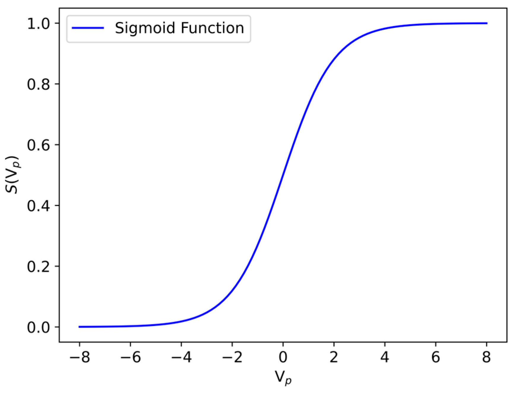
The description of the p-th bit-string, $x_{p,s}^{q, \mathrm{n}\mathrm{e}\mathrm{x}\mathrm{t}}$, in Equation (22) results in a real number, whilst its determination as a binary number is required. Hence, the movement of particles is carried out by converting the real number within the interval $\left[0, 1\right]$ to a binary space. The so-called sigmoid function, $\mathcal{S}\left(v_{p,s}^{q, \mathrm{n}\mathrm{e}\mathrm{x}\mathrm{t}}\right)$, indicating the S-shape parametric transfer in Figure 1, becomes:

$$\mathcal{S}\left(v_{p,s}^{q, \mathrm{n}\mathrm{e}\mathrm{x}\mathrm{t}}\right)=\mathrm{S}\mathrm{i}\mathrm{g}\mathrm{m}\mathrm{o}\mathrm{i}\mathrm{d}\left(v_{p,s}^{q, \mathrm{n}\mathrm{e}\mathrm{x}\mathrm{t}}\right)=\frac{1}{1+e^{-\left(v_{p,s}^{q, \mathrm{n}\mathrm{e}\mathrm{x}\mathrm{t}}\right)}}.$$

(25)

The velocity, $v_{p,s}^{q, \mathrm{n}\mathrm{e}\mathrm{x}\mathrm{t}}$, is converted to the S-shape, $\mathcal{S}\left(v_{p,s}^{q, \mathrm{n}\mathrm{e}\mathrm{x}\mathrm{t}}\right),$ value with an interval $\left[0, 1\right]$. The q-th bit-string, $x_{p,s}^{q, \mathrm{n}\mathrm{e}\mathrm{x}\mathrm{t}}$, can be updated from $\mathcal{S}\left(v_{p,s}^{q, \mathrm{n}\mathrm{e}\mathrm{x}\mathrm{t}}\right)$ using the following probabilistic function:

$$x_{p,s}^{q, \mathrm{n}\mathrm{e}\mathrm{x}\mathrm{t}}=\left\{\begin{array}{c}1 \mathrm{i}\mathrm{f} {r3}_p>\mathcal{S}\left(v_{p,s}^{q, \mathrm{n}\mathrm{e}\mathrm{x}\mathrm{t}}\right)\\ 0 \mathrm{i}\mathrm{f} {r3}_p\le \mathcal{S}\left(v_{p,s}^{q, \mathrm{n}\mathrm{e}\mathrm{x}\mathrm{t}}\right)\end{array}\right.,$$

(26)

where ${ r3}_p$ is a uniform random number within an interval $\left[0, 1\right]$.

It is worthwhile mentioning that a range of transfer functions, including U-, Z-, X-, S-, and V-shape [47], are made available, and they all are compatible for the implementation in this work. Given its superior performance reported in the literature [48], the S-shape transfer function is adopted by the proposed method. Nevertheless, it is important to emphasize that this work can be readily applied to any type of transfer function.

The set of bit-strings, $\mathrm{𝓃}s$, exemplars of the p-th particle is determined. Thus, the steel sections are specified as $\mathrm{𝓃}g$ independent member groups, and the associated section properties are specified as ${\mathbf{a}}^p$. Hence, the objective function, $\mathcal{W}\left({\mathbf{a}}^p\right)$, in Equation (1) is calculated for the constructed p-th particle. In this study $\mathrm{𝓃}s=ng$. The best position, ${\mathbf{X}}_p^{\mathrm{b}\mathrm{e}\mathrm{s}\mathrm{t}}$, is the position of the p-th particle that yields the most optimal $\mathcal{W}\left({\mathbf{a}}^p\right)$ solution for all design iterations. The global best position, ${\mathbf{X}}^{\mathrm{G}\mathrm{l}\mathrm{o}\mathrm{b}\mathrm{a}\mathrm{l}}$, is ${\mathbf{X}}_p^{\mathrm{b}\mathrm{e}\mathrm{s}\mathrm{t}}$, giving the most optimal solution, $\mathcal{W}\left({\mathbf{a}}^p\right)$, for all $\mathrm{𝓃}p$ particles.

To enhance the cross-particle searching ability of a standard PSO method, the comprehensive learning strategy is carried out [49]. The technique encourages each p-th particle to learn from the best exemplars of other particles in the same dimension. The approach constructs a diverse swarm and increases the likelihood of obtaining accurate optimal solutions.

The best position, ${\mathbf{X}}_p^{\mathrm{b}\mathrm{e}\mathrm{s}\mathrm{t}}$, is further determined via the new learning exemplar, ${\mathbf{X}}_{p,f}^{\mathrm{b}\mathrm{e}\mathrm{s}\mathrm{t}}\in {\mathfrak{R}}^{\mathrm{𝓃}s}=\left(X_{p,f\left(s\right)}^{\mathrm{b}\mathrm{e}\mathrm{s}\mathrm{t}}|\forall s\in \left\{1,2,\cdots ,\mathrm{𝓃}s\right\}\right)$. For the specific p-th particle, the learning exemplar, ${\mathbf{X}}_{p,f}^{\mathrm{b}\mathrm{e}\mathrm{s}\mathrm{t}}$, is initially assigned the best positions, ${\mathbf{X}}_p^{\mathrm{b}\mathrm{e}\mathrm{s}\mathrm{t}}$. 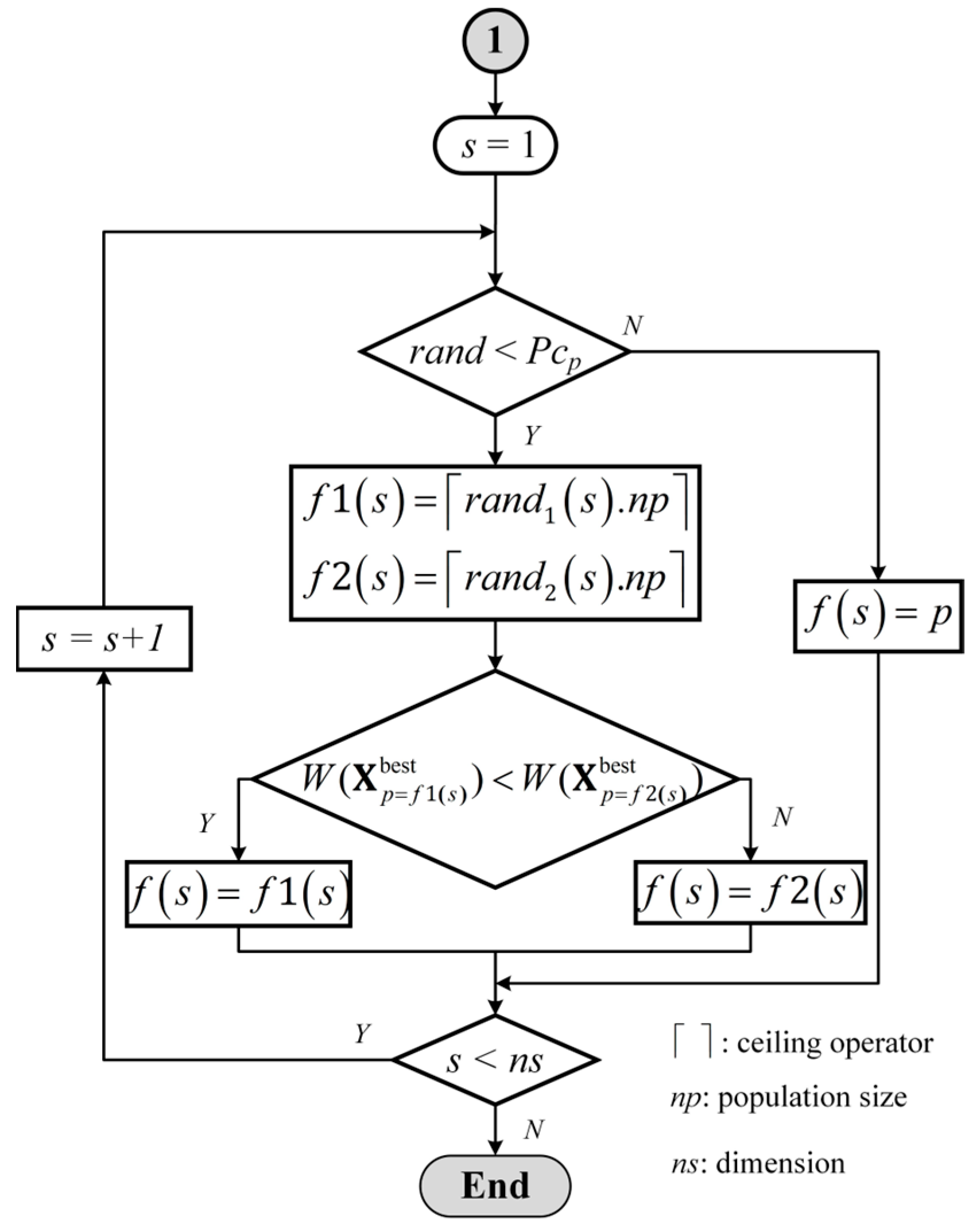The location of the best particle, $X_{p,f\left(s\right)}^{\mathrm{b}\mathrm{e}\mathrm{s}\mathrm{t}}$, is defined by the particle index, $f\left(s\right)$, through the learning probability searches across all $\mathrm{𝓃}p$ particles in the same s-th dimension. Subsequently, for each s-th dimension, the exemplar, ${\mathbf{X}}_{p,f}^{\mathrm{b}\mathrm{e}\mathrm{s}\mathrm{t}}$, of the p-th particle explores the new $X_{p,f\left(s\right)}^{\mathrm{b}\mathrm{e}\mathrm{s}\mathrm{t}}$ from one of the two best particles $\left(X_{p,f1\left(s\right)}^{\mathrm{b}\mathrm{e}\mathrm{s}\mathrm{t}},X_{p,f2\left(s\right)}^{\mathrm{b}\mathrm{e}\mathrm{s}\mathrm{t}}\right)$ where $X_{p,f1\left(s\right)}^{\mathrm{b}\mathrm{e}\mathrm{s}\mathrm{t}}\ne X_{p,f2\left(s\right)}^{\mathrm{b}\mathrm{e}\mathrm{s}\mathrm{t}}$. Each $X_{p,f1\left(s\right)}^{\mathrm{b}\mathrm{e}\mathrm{s}\mathrm{t}} \mathrm{a}\mathrm{n}\mathrm{d} X_{p,f2\left(s\right)}^{\mathrm{b}\mathrm{e}\mathrm{s}\mathrm{t}}$ is randomly chosen from the present ${\mathbf{X}}_p^{\mathrm{b}\mathrm{e}\mathrm{s}\mathrm{t}}$ collection for all $p\in \left\{1,2,\cdots ,\mathrm{𝓃}p\right\}$ populations, viz., $\left(X_{p=1,s}^{\mathrm{b}\mathrm{e}\mathrm{s}\mathrm{t}},\dots ,X_{p=np,s}^{\mathrm{b}\mathrm{e}\mathrm{s}\mathrm{t}}\right)$. The index, $f\left(s\right)$, then reads either $f1\left(s\right)$ or $f2\left(s\right)$ related to the more optimal objective function value, namely, $\mathrm{m}\mathrm{i}\mathrm{n}\left(\mathcal{W}\left({\mathbf{X}}_{p=f1\left(s\right)}^{\mathrm{b}\mathrm{e}\mathrm{s}\mathrm{t}}\right),\mathcal{W}\left({\mathbf{X}}_{p=f2\left(s\right)}^{\mathrm{b}\mathrm{e}\mathrm{s}\mathrm{t}}\right)\right)$. The new exemplar in the s-th dimension is thus updated by $X_{p,f\left(s\right)}^{\mathrm{b}\mathrm{e}\mathrm{s}\mathrm{t}}=X_{p=f\left(s\right),s}^{\mathrm{b}\mathrm{e}\mathrm{s}\mathrm{t}}$. This process is repeated for all $\mathrm{𝓃}s$ dimensions, allowing the specific p-th particles to comprehensively explore the new directions, ${\mathbf{X}}_{p,f}^{\mathrm{b}\mathrm{e}\mathrm{s}\mathrm{t}}$, see Figure 2.

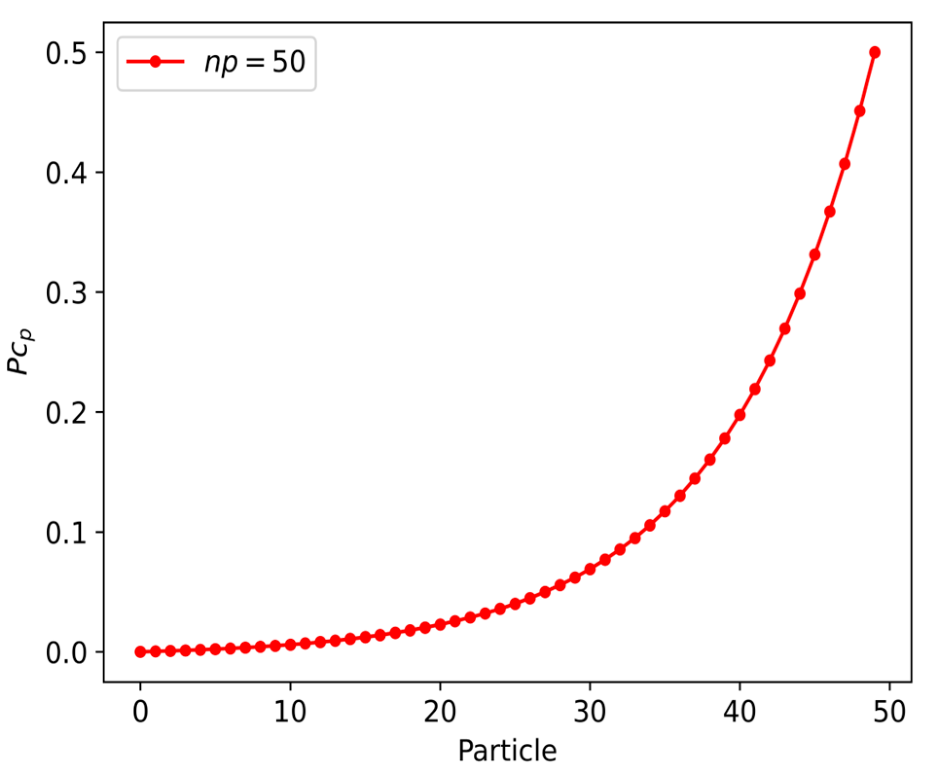
The learning probability function, ${Pc}_P$, as in Equation (27) [38], is utilized. The new learning position of an exemplar $\left(X_{p,f\left(s\right)}^{\mathrm{b}\mathrm{e}\mathrm{s}\mathrm{t}}{=X}_{p=f\left(s\right),s}^{\mathrm{b}\mathrm{e}\mathrm{s}\mathrm{t}}\right)$ of the p-th particle is updated only if the random number within an interval $\left[0, 1\right]$ (called rand) is less than the ${Pc}_P$ value. The spectrum of ${Pc}_P$ values, generated for $\mathrm{𝓃}p=50$ particles, is depicted in Figure 3.

$${Pc}_P=\frac{1}{20}+\frac{9}{20}\frac{\left(e^{\left(\raisebox{1ex}{$10\left(p-1\right)$}\!\left/ \!\raisebox{-1ex}{$\mathrm{𝓃}p-1$}\right.\right)}-1\right)}{e^{\left(10\right)}-1}.$$

(27)

In the case where an exemplar remains at its best position ($X_{p,f\left(s\right)}^{\mathrm{b}\mathrm{e}\mathrm{s}\mathrm{t}}=X_{p,s}^{\mathrm{b}\mathrm{e}\mathrm{s}\mathrm{t}}$ for $\forall s\in \left\{1,2,\cdots ,\mathrm{𝓃}s\right\}$), the new position, ${\mathbf{X}}_{p,f}^{\mathrm{b}\mathrm{e}\mathrm{s}\mathrm{t}}$, is randomly selected from the exemplars of some other particle in the same s-th dimension.

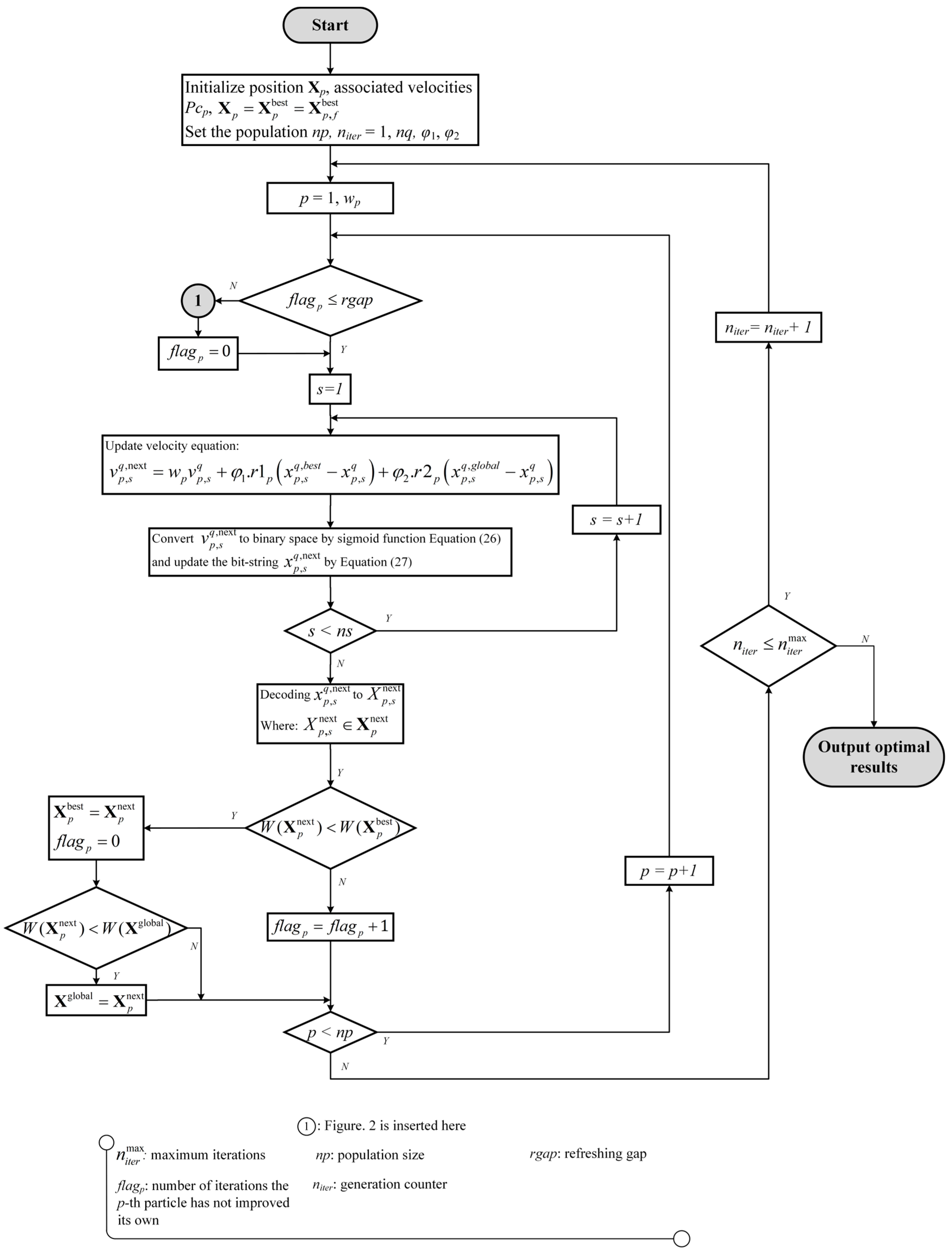
Comprehensive learning searches are implemented when there is no improvement in the objective function for more than a specified number of iterations, i.e., when rgap = 5. This outcome is referred to as a refreshing gap parameter (rgap) [38].

The pseudocode for the proposed BCLPSO method can be summarized by the flowchart in Figure 4.

4. Inertial Weight Parameters

The influence of an inertia weight parameter, $w_p$, in Equation (25) on the performance of the BCLPSO algorithm is investigated. In

Table 1. Benchmark functions.

Function	Optimization Formulation	Range
$f\left(x\right)$1: Sphere’s	$\min f\left(x\right)={\displaystyle \sum _{i=1}^n}{x}_i^2$	[−100, 100]
$f\left(x\right)$2: Rosenbrock’s	$\min f\left(x\right)={\displaystyle \sum _{i=1}^{n-1}}\left[100\right(x_{i+1}-x_i^2{)}^2+(x_i-1{)}^2]$	[−200, 200]
$f\left(x\right)$3: Rastrigin’s	$\min f\left(x\right)=10n+{\displaystyle \sum _{i=1}^n}[x_i^2-10\cos \left(2\pi x_i\right))]$	[−5.12, 5.12]
$f\left(x\right)$4: Griewank’s	$\min f\left(x\right)=\frac{1}{4000}{\displaystyle \sum _{i=1}^n}{x}_i^2-{\displaystyle \prod _{i=1}^n}cos\left(\frac{x_i}{\sqrt{i}}\right)+1$	[−600, 600]
$f\left(x\right)$5: Schaffer’s	$\min f\left(x\right)=0.5-\frac{(\sin \sqrt{x_1^2+x_2^2}{)}^2-0.5}{[1+0.001(x_1^2+x_2^2){]}^2}$	[−100, 100]
$f\left(x\right)$6: Ackley’s	$\min f\left(x\right)=-20\exp \left(-0.2\sqrt{\frac{1}{n}}{\displaystyle \sum _{i=1}^n}{x}_i^2\right)-exp\left(\frac{1}{n}{\displaystyle \sum _{i=1}^n}\cos \left(2\pi x_i\right)\right)+20+e$	[−32, 32]

, six optimization benchmark functions [50] are solved, using the proposed BCLPSO method. The minimum value of the function $f\left(x\right)$ is set to 0. The inertia weight parameter is selected as the constant within the interval [0.9, 1.02], as well as the linear decreasing value from 0.9 to 0.4. Each function was solved 50 times. Each solve proceeds 6000 analyses. The set of unknown variables, selected from the range between 2 and 10, requires 15 bits to accommodate the available design domains. The BCLPSO algorithm incorporated 50 swarm populations.

In

Table 2. Minimum fitness of benchmark functions.

Inertial Weight	$\mathit{f}\left(\mathit{x}\right)$1	$\mathit{f}\left(\mathit{x}\right)$2	$\mathit{f}\left(\mathit{x}\right)$3	$\mathit{f}\left(\mathit{x}\right)$4	$\mathit{f}\left(\mathit{x}\right)$5	$\mathit{f}\left(\mathit{x}\right)$6
0.90	3.75	7801.85	7.34	0.80	0.00246	1.70
0.92	1.63	477.33	6.17	0.64	0.00246	0.63
0.94	0.12	90.24	1.28	0.27	0.00246	0.25
0.96	0.00434	9.53	0.01	0.11	0.00246	0.03
0.98	9.32 × 10−5	6.96	4.84 × 10−5	0.01	0.00246	3.96 × 10−3
1.00	9.32 × 10−5	7.34	1.24	0.03	0.00246	3.96 × 10−3
1.02	9.32 × 10−5	8.26	2.00	0.01	0.00246	3.96 × 10−3
0.4 to 0.9	113.39	1,958,397.03	24.41	1.73	0.00246	4.92

and

Table 3. Standard deviation of minimum fitness of benchmark functions.

Inertial Weight	$\mathit{f}\left(\mathit{x}\right)$1	$\mathit{f}\left(\mathit{x}\right)$2	$\mathit{f}\left(\mathit{x}\right)$3	$\mathit{f}\left(\mathit{x}\right)$4	$\mathit{f}\left(\mathit{x}\right)$5	$\mathit{f}\left(\mathit{x}\right)$6
0.90	4.59	37877.70	2.77	0.08	107.24	0.44
0.92	1.02	8692.70	2.26	0.10	100.66	0.44
0.94	0.21	3975.95	1.96	0.11	112.51	0.11
0.96	0.01	786.38	1.66	0.09	105.87	0.02
0.98	0.00	460.86	1.32	0.05	85.59	0.00
1.00	0.00	4190.81	3.74	0.06	153.08	0.71
1.02	0.00	3823.98	3.12	0.11	126.80	0.90
0.4 to 0.9	110.80	6,036,157.12	4.69	0.69	113.13	1.05

, the optimal solutions, i.e., the minimum fitness and standard deviations of the benchmark functions are given. The solutions associated with the constant inertial weight of 0.98 present the most optimal values as well as the smallest standard deviations for all problems considered. In contrast, the results obtained by the design adopting the linear decreasing inertia weight (from 0.9 to 0.4) produce the lowest optima with large standard deviations. Thus, it is noted that the BCLPSO uses the inertia weight of 0.98 for all the examples illustrated in this paper.

5. Illustrative Examples

Herein, three examples of structural optimization demonstrate optimal designs for moment-resisting steel frames with and without cross-brace members. The design process determines the minimum member sizes from 267 standard steel W-sections. Each section is coded by standard notations. For example, a W21 × 44 section indicates the wide flange section comprising of an approximate depth of 21 inches and weight of 44 lb/ft. The W-sections are widely employed not only for columns but also for beams. The discrete optimization problem in Equation (1) complies with the AISC-LRFD specifications [29]. Examples 2 and 3 incorporate the influence of geometry nonlinearity, ($P-\delta$) and ($P-∆$). The proposed BCLPSO method incorporates 50 swarm particles and 20,000 analyses. This approach is independently performed 50 times to illustrate the reliability of the design.

It is worthwhile noting that the steel structural designs considered in this work are set up to contain similar criteria to the available literature and benchmarks [18,26,51], where the local buckling of steel (generally known as non-compact and slender) sections, is not considered. The proposed method can be further adopted to accommodate the design of non-compact and slender sections, complying with standard design (e.g., AISC, Eurocode 3, etc.) specifications. Adjustment to Equations (5)–(11) is required to address the formulations stated in the relevant design specifications. The proposed BCLPSO algorithm was encoded as a MATLAB code, made available for download at https://github.com/Rut44139/BCLPSO (accessed on 30 July 2023).

5.1. Example 1: Two-Bay, Three-Story Frame

In Figure 5, example 1 depicts a two-bay, three-story frame under applied forces [52]. The structure was designed to comply with ultimate strength conditions. The material properties used include the modulus of elasticity ($E=\mathrm{29,000} \mathrm{k}\mathrm{s}\mathrm{i})$ and yield stress ${(F}_y=36 \mathrm{k}\mathrm{s}\mathrm{i})$. The discrete frame model consists of 15 elements, classified into two member groups: one for all beams and the other for all columns. The beam group was designed in accordance with the set of 267 standard W-shape sections. The column group was acquired for a set of 18 available W10 sections. The effective length factors for all members were $K_x=1.0$ and $K_y=1.0$. The unbraced lengths of all brace members were 1/6 of their physical lengths.

The proposed BCLPSO method selects nine bits for a beam element and five bits for a column. The total number of possible member selections can reach up to $2^{14}$ combinations. In

Table 4. Example 1: optimal solutions obtained via various design methods.

Design Group	Benchmark	GA [18]	ACO [28]	SBO [26]	Present Work
Beam	W24 × 62	W24 × 62	W24 × 62	W24 × 62	W24 × 62
Column	W10 × 60	W10 × 60	W10 × 60	W10 × 60	W10 × 60
Best weight (lb)	18,792	18,792	18,792	18,792	18,792
Mean (lb)	n/a	22,080	19,163	18,792	18,792
SD	n/a	5818	1693	0	0
No. of analyses	n/a	900	880	502	3
No. of runs	n/a	30	100	100	50

Note: GA = genetic algorithm; ACO = ant colony optimization; SBO = school-based optimization.

, the minimum weight of 18,792 lb is compared with those reported by GA [18], ACO [28], and SBO [26]. The accuracy of the present design solution is clearly expressed in Table 4. Moreover, the statistical values collected from 50 independent designs signified a zero standard deviation value, illustrating for this academic benchmark that the optimal design can be reliably replicable. In Figure 6, fast solution convergence can be observed, where the total design weight reduces sharply within the first 50 analyses. In Equation (3), the ultimate strength ratios, $\left|{\sigma }_l\right|$, developed for all design members under the applied forces, strictly comply with the limits (viz., $\left|{\sigma }_l\right|\le 1$), see Figure 7.

5.2. Example 2: One-Bay, Ten-Story Frame

Example 2 outlines one-bay, ten-story moment-resisting frames, under applied forces (Figure 8). The unbraced frame is displayed in Figure 8a. The braced frames are depicted in Figure 8b,c with different configurations of member groups. The structure is designed with and without cross braces to comply with the ultimate strength and limited displacement conditions, simultaneously. The material properties utilized include the modulus of elasticity $(E=\mathrm{29,000} \mathrm{k}\mathrm{s}\mathrm{i})$ and yield stress ${(F}_y=36 \mathrm{k}\mathrm{s}\mathrm{i})$.

The discrete frame model consists of 30 beam and column members. The beam group was planned to comply with a set of 267 standard W-shape sections. The column group was devised from a set of 66 available W14- and W12-sections. The braced member group was undertaken via a set of 33 available W6- to W10-sections. The effective length factors of all members were $K_x=1.0$ and $K_y=1.0$. The unbraced lengths for all brace members were ½ of their physical lengths.

Table 5. Example 2: geometry and design conditions of structures in all cases.

Case	Geometry	Figure	Drift Constraint
1	Unbraced frame	Figure 8a	0.400 in at top-roof
2	Unbraced frame	Figure 8a	4.920 in at all stories
3	Braced frame	Figure 8b	4.920 in at all stories
4	Braced frame	Figure 8c	4.920 in at all stories

describes the geometry, member groups, and drift constraints applied to four frame design cases. The proposed BCLPSO method successfully determined the optimal solutions for all structures in the design cases. In

Table 6. Example 2: optimal design solutions for case 1.

Member Group	ACO [28]	TLBO [24]	SBO [26]	Present Work
1	W14 × 233	W14 × 233	W14 × 233	W14 × 233
2	W14 × 176	W14 × 176	W14 × 176	W14 × 176
3	W14 × 145	W14 × 145	W14 × 145	W14 × 145
4	W14 × 99	W14 × 99	W14 × 99	W14 × 99
5	W12 × 65	W12 × 65	W14 × 61	W14 × 61
6	W30 × 108	W30 × 108	W30 × 108	W30 × 108
7	W30 × 90	W30 × 90	W30 × 90	W30 × 90
8	W27 × 84	W27 × 84	W27 × 84	W27 × 84
9	W21 × 44	W21 × 44	W18 × 46	W18 × 46
Best weight (lb)	62,562	62,562	62,430	62,430
Mean (lb)	63,308	-	63,244	63,907
SD (lb)	684	-	706.84	1190
No. of analyses	8300	4000	11,677	5408
No. of runs	100	-	100	50

Note: ACO = ant colony optimization; TLBO = teaching–learning-based optimization; SBO = school-based optimization.

,

Table 7. Example 2: optimal design solutions for case 2.

Member Group	GA [18]	SBO [26]	Present Work
1	W14 × 233	W14 × 233	W14 × 233
2	W14 × 176	W14 × 176	W14 × 176
3	W14 × 159	W14 × 159	W14 × 159
4	W14 × 99	W14 × 99	W14 × 99
5	W12 × 79	W14 × 61	W14 × 61
6	W33 × 118	W33 × 118	W33 × 118
7	W30 × 90	W30 × 90	W30 × 90
8	W27 × 84	W27 × 84	W27 × 84
9	W24 × 55	W18 × 46	W18 × 46
Best weight (lb)	65,136	64,002	64,002
Mean (lb)	-	65,880	65,806
SD (lb)	-	832.95	1123
No. of analyses	3000	12,691	4647
No. of runs	-	100	50

Note: GA = genetic algorithm; SBO = school-based optimization.

,

Table 8. Example 2: optimal design solutions for case 3.

Member Group	Present Work
1	W14 × 211
2	W14 × 159
3	W14 × 132
4	W14 × 99
5	W14 × 61
6	W27 × 84
7	W24 × 84
8	W30 × 90
9	W18 × 46
10	W8 × 24
12	W8 × 24
14	W10 × 22
Best weight (lb)	62,224
Mean (lb)	65,228
SD (lb)	1668
No. of analyses	4852
No. of runs	50

and

Table 9. Example 2: optimal design solutions for case 4.

Member Group	Present Work
1	W14 × 145
2	W14 × 211
3	W12 × 210
4	W14 × 159
5	W12 × 152
6	W14 × 99
7	W12 × 120
8	W12 × 96
9	W14 × 68
10	W14 × 53
11	W30 × 90
12	W30 × 116
13	W33 × 118
14	W30 × 99
15	W27 × 84
16	W24 × 68
17	W27 × 84
18	W24 × 76
19	W24 × 76
20	W21 × 44
21	W8 × 24
26	W8 × 18
Best weight (lb)	60,805
Mean (lb)	65,028
SD (lb)	1819
No. of analyses	17,078
No. of runs	50

, the minimum total weight solutions, optimal member sizes/distributions, and statistical (i.e., mean and standard deviation) values associated with the 50 independent designs are reported. The accuracy (optimality) of the computed design results is verified via comparison with the literature [18,24,26,28], which reported the minimum weight designs of unbraced frames in cases 1 and 2 (see Table 6 and Table 7, respectively). The lowest total weight of the structure designed by the BCLPSO approach presents the most minimum. The corresponding standard deviations and mean total weight values are small and comparable with those obtained by the SBO [26]. However, the total number of analyses demonstrated by the BCLPSO was approximately half of what was obtained by the SBO. It is evident that these results reveal the reliability of the proposed design method in obtaining replicable design solutions at modest computing efforts.

In Figure 9, the successful convergence revealing the optimal total weight solutions for all cases is depicted. In all cases, the minimum total weights of the designed structures were achieved approximately within the first 10,000 analyses (viz., half of the total preset number of analyses). In Figure 10, the optimal brace layouts in cases 3 and 4 are depicted. Moreover, the ultimate strength ratios, $\left|{\sigma }_l\right|$, of all design members as well as lateral displacements are plotted (Figure 11 and Figure 12). Such results verify that the ultimate strength and limited sway deformation constraints fully complied with the optimally designed structures in all cases.

5.3. Example 3: Three-Bay, Twenty Four-Story Frame

In Figure 13, the final example examines the three-bay, twenty four-story frames with and without brace members [53]. The frames are designed to comply with standard AISC-LRFD specifications, i.e., ultimate strength conditions and limited sway displacements of 0.480 in for all stories.

This model consists of 168 beam and column elements. The beam members are selected from the set of 267 standard steel W-sections, and the columns are selected from the set of 37 steel W14-sections. The material properties employed are the modulus of electricity $(E=\mathrm{29,732} \mathrm{k}\mathrm{s}\mathrm{i})$ and the yield stress $(F_y=33.4 \mathrm{k}\mathrm{s}\mathrm{i})$. The unbraced lengths of all beams and columns are their physical lengths ($K_x=1.0$ and $K_y=1.0$). The design members are categorized into a number of independent groups as depicted in Figure 13. Design conditions for both unbraced and braced frames are detailed in

Table 10. Example 3: geometry and design conditions of structures for all cases.

Case	Structure	Figure	Drift Constraint
1	Unbraced frame	Figure 13a	0.480 in at all stories
2	Braced frame	Figure 13b	0.480 in at all stories
3	Braced frame	Figure 13c	0.480 in at all stories

.

The unbraced and braced frames in cases 1 to 3 are successfully designed to determine the optimal member sizes and brace layouts (in cases 2 and 3) by performing the proposed BCLPSO method. The optimal solutions (including the minimum total weights, steel sections, and average and standard deviation values associated with 50 independent designs) are summarized in

Table 11. Example 3: optimal design solutions for case 1.

Member Group	ES-DE [51]	CBO [21]	HBMO [23]	SBO [26]	Present Work
1	W30 × 90	W27 × 102	W10 × 22	W30 × 90	W30 × 90
2	W21 × 55	W8 × 18	W27 × 539	W8 × 18	W8 × 18
3	W21 × 48	W24 × 55	W8 × 21	W24 × 55	W21 × 48
4	W10 × 45	W6 × 8.5	W33 × 221	W6 × 8.5	W10 × 12
5	W14 × 145	W14 × 132	W14 × 145	W14 × 193	W14 × 159
6	W14 × 109	W14 × 120	W14 × 145	W14 × 145	W14 × 120
7	W14 × 99	W14 × 145	W14 × 68	W14 × 120	W14 × 109
8	W14 × 145	W14 × 82	W14 × 22	W14 × 82	W14 × 61
9	W14 × 109	W14 × 61	W14 × 48	W14 × 53	W14 × 48
10	W14 × 48	W14 × 43	W14 × 68	W14 × 53	W14 × 48
11	W14 × 38	W14 × 38	W14 × 132	W14 × 38	W14 × 43
12	W14 × 30	W14 × 22	W14 × 342	W14 × 22	W14 × 26
13	W14 × 99	W14 × 99	W14 × 159	W14 × 120	W14 × 99
14	W14 × 132	W14 × 109	W14 × 109	W14 × 132	W14 × 109
15	W14 × 109	W14 × 82	W14 × 99	W14 × 120	W14 × 99
16	W14 × 68	W14 × 90	W14 × 48	W14 × 109	W14 × 120
17	W14 × 68	W14 × 74	W14 × 43	W14 × 99	W14 × 99
18	W14 × 68	W14 × 61	W14 × 53	W14 × 61	W14 × 61
19	W14 × 61	W14 × 30	W14 × 176	W14 × 34	W14 × 43
20	W14 × 22	W14 × 22	W14 × 211	W14 × 19	W14 × 26
Weight (lb)	212,988	215,874	214,848	216,306	205,056
Mean (lb)	n/a	225,071	n/a	224,310	224,152
SD (lb)	n/a	n/a	888	6855	15,475
No. of analyses	12,500	15,360	2074	14,817	6890
No. of runs	20	30	50	100	50

Note: ES-DE = eagle strategy with differential evolution; CBO = colliding bodies optimization; HBMO = honey bee mating optimization; SBO = school-based optimization.

,

Table 12. Example 3: optimal design solutions for case 2.

Member Group	Present Work	Member Group	Present Work	Member Group	Present Work	Member Group	Present Work
1	W16 × 36	13	W14 × 53	34	W8 × 15	66	W10 × 15
2	W8 × 18	14	W14 × 43	37	W8 × 15	69	W8 × 18
3	W10 × 22	15	W14 × 43	41	W8 × 18	72	W8 × 21
4	W8 × 10	16	W14 × 48	45	W10 × 39	73	W10 × 30
5	W14 × 99	17	W14 × 30	46	W10 × 30	79	W8 × 24
6	W14 × 99	18	W14 × 30	50	W8 × 18	81	W10 × 26
7	W14 × 61	19	W14 × 43	53	W10 × 19	83	W10 × 22
8	W14 × 68	20	W14 × 43	54	W8 × 28	84	W8 × 18
9	W14 × 68	23	W10 × 22	55	W6 × 9	87	W8 × 31
10	W14 × 43	27	W10 × 22	58	W8 × 28
11	W14 × 48	28	W8 × 35	62	W8 × 13
12	W14 × 22	32	W10 × 22	64	W8 × 10
Weight (lb)				132,972
Mean (lb)				176,326
SD (lb)				18,187
No. of analyses				18,139
No. of runs				50

and

Table 13. Example 3: optimal design solutions for case 3.

Member Group	Present Work	Member Group	Present Work	Member Group	Present Work	Member Group	Present Work
1	W12 × 26	12	W14 × 43	23	W8 × 18	64	W10 × 12
2	W24 × 62	13	W14 × 30	27	W10 × 22	72	W8 × 31
3	W14 × 22	14	W14 × 22	28	W8 × 21	73	W10 × 49
4	W12 × 26	15	W14 × 43	34	W8 × 18	75	W10 × 26
5	W12 × 16	16	W14 × 43	50	W8 × 18	78	W10 × 26
6	W16 × 31	17	W14 × 43	53	W8 × 13	79	W8 × 35
7	W14 × 120	18	W14 × 43	56	W10 × 26	81	W8 × 21
8	W14 × 82	19	W14 × 43	60	W8 × 15	83	W8 × 18
9	W14 × 99	20	W14 × 43	61	W8 × 15	89	W10 × 17
10	W14 × 61	21	W14 × 30	62	W6 × 9	90	W10 × 19
11	W14 × 48	22	W14 × 48	63	W10 × 12
Weight (lb)				138,050
Mean (lb)				178,475
SD (lb)				17,873
No. of analyses				19,595
No. of runs				50

for cases 1 to 3, respectively. The accuracy of the minimum total weight results, computed by the BCLPSO, is evidenced by case 1 (see Table 11) through the good comparison with various benchmarks [21,23,26,51]. In this case, the best minimum weight and its average value present the most optimal solutions. It is noted that the computing efforts required to converge the optimal solution are modest.

In Figure 14, the convergence plots describe that the total design weights decrease and converge to the optimal values in all cases. In Figure 15, the optimal brace layouts of cases 2 and 3 are outlined. In essence, all optimal designs strictly satisfy AISC-LRFD specifications. In Figure 16 and Figure 17, the plots of ultimate strength ratios, $\left|{\sigma }_l\right|$, and the lateral sway displacements are depicted. It is also observed that the presence of cross braces designed in cases 2 and 3 saves on the total optimal weights (material costs) by some 35% and 32% as compared to the unbraced frame in case 1.

5.4. Discussions of the Results

From the successfully solved optimal solutions of Section 5.1, Section 5.2 and Section 5.3, three pertinent comments are briefly discussed.

(i)

The proposed BCLPSO method incorporates various enhanced search techniques. It utilizes the learning probability function that facilitates cooperative responses among swarm populations. Moreover, the discrete search space can be directly mapped into binary bit-strings using the sigmoid function within a decoding environment. The inertial weight parameter of 0.98 presents the most appropriate value enabling the good performance of the BCLPSO approach among all benchmarks tested in Table 5.

(ii)

The optimal solutions computed by the BCLPSO method in examples 1 to 3 are summarized in

Table 14. Result summary for the lowest minimum weight designs.

Example	Present Work (lb)	No. of Analyses	Reference Method (lb)	No. of Analyses	Reference
1	18,792	3	18,792	900	GA [18]
2 Case 1	62,430	5408	62,430	11,677	SBO [26]
2 Case 2	64,002	4647	64,002	12,691	SBO [26]
3 Case 1	205,056	6890	212,988	12,500	ES-DE [51]

. The table presents the good performance of the proposed BCLPSO method in determining the minimum weight designs with significantly less computing efforts as compared to those reported in the literature [18,26,51]. More explicitly, the lowest minimum total weight of 205,056 lb (some 3% reduction) can be achieved by performing only 6890 BCLPSO analyses (44% smaller), whilst the ES-DE [51] approach results in the total weight of 212,988 lb with 12,500 analyses. The statistical (standard deviation and mean) values collected from 50 independent BCLPSO runs are small and evidence the reliability of the proposed method in obtaining the replicable optimal solutions for different initial parametric setups.

(iii)

Figure 6, Figure 9 and Figure 14 illustrate the fast convergence of the total weight designs to reach the minimum solutions (both the lowest and mean values), where the total number of analyses involved to obtain optimality is modest. However, the decoding of bit-string (0 and 1) variables within a binary space expands the search domain (containing fake variables), and is likely subjected to the presence of nonlinearity leading to local optima. Future research can focus on optimizing the values from fake available solutions. Handling large-scale optimization problems necessitates a high-performance parallel computing framework with ample memory storage. Incorporating the machine learning-based techniques that construct the so-called surrogate-assisted predictive models of design structures can bypass the need for iterative finite element implementations under time-consuming metaheuristic procedures. Exploring the latter approach is an interesting avenue for future extension work.

6. Conclusions

In this paper, the BCLPSO method demonstrates its effectiveness in determining the optimal design for nonlinear discrete steel structures. Such a design complies with ASC-LRFD specifications. It is noted that BCLPSO decodes the intrinsic binary variables of bit sizes to explicitly define individual discrete steel sections. The optimal solutions computed are as meaningful as those of the challenging nonlinear integer programming problem, but the computing efforts taken by the proposed approach are modest. Moreover, the comprehensive learning strategy incorporated within the swarm optimization algorithm enables the cross-particle searches to test the global best particle and the likelihood to overcome local optimal pitfalls.

Six benchmarks based on the nonlinear optimization formulations have been processed by the BCLPSO method with various inertia weight parameters, $w_p$. The value of $w_p=0.98$ presents the most superior performance (in terms of solution accuracy and reliability) for all benchmarks tested. Three structural design examples considering the in-plane moment-resisting steel frames with and without braces were successfully carried out by the proposed BCLPSO approach. The optimal steel sections and brace layouts were determined from the standard steel sections. The accuracy of the optimal design solutions has also been validated via comparison with the literature. The computing efforts required to successfully converge the optimal designs of structures in all cases are proved to be modest. The statistical (mean and standard deviation) values associated with 50 independent designs indicate the robustness of the proposed BCLPSO approach, where the minimum total weight solutions can be replicable.

References

1. Liang, Q.Q.; Xie, Y.M.; Steven, G.P. Topology optimization of strut-and-tie models in reinforced concrete structures using an evolutionary procedure. ACI Struct. J. 2000, 97, 322–330. [Google Scholar] [CrossRef] [Green Version]
2. Rong, J.H.; Liang, Q.Q. A level set method for topology optimization of continuum structures with bounded design domains. Comput. Methods Appl. Mech. Eng. 2008, 197, 1447–1465. [Google Scholar] [CrossRef]
3. Van, T.H.; Tangaramvong, S.; Limkatanyu, S.; Xuan, H.N. Two-phase ESO and comprehensive learning PSO method for structural optimization with discrete steel sections. Adv. Eng. Softw. 2022, 167, 103102. [Google Scholar] [CrossRef]
4. Kim, Y.C.; Mortazavi, S.J.; Farzampour, A.; Hu, J.W.; Mansouri, I.; Awoyera, P.O. Optimization of the Curved Metal Damper to Improve Structural Energy Dissipation Capacity. Buildings 2022, 12, 67. [Google Scholar] [CrossRef]
5. Farzampour, A.; Khatibinia, M.; Mansouri, I. Shape optimization of butterfly-shaped shear links using grey wolf algorithm. Ing. Sismica 2019, 36, 27–41. [Google Scholar]
6. Farzampour, A.; Mansouri, I.; Dehghani, H. Incremental Dynamic Analysis for Estimating Seismic Performance of Multi-Story Buildings with Butterfly-Shaped Structural Dampers. Buildings 2019, 9, 78. [Google Scholar] [CrossRef] [Green Version]
7. Farzampour, A.; Mansouri, I.; Mortazavi, S.J.; Hu, J.W. Force–Displacement Relationship of the Butterfly-Shaped Beams Based on Gene Expression Programming. Int. J. Steel. Struct. 2020, 20, 2009–2019. [Google Scholar] [CrossRef]
8. Farzampour, A. Structural behavior prediction of the Butterfly-shaped and straight shear fuses. Structures 2021, 33, 3964–3972. [Google Scholar] [CrossRef]
9. Farzampour, A.; Eatherton, M.R.; Mansouri, I.; Hu, J.W. Effect of flexural and shear stresses simultaneously for optimized design of butterfly-shaped dampers: Computational study. Smart Struct. Syst. 2019, 23, 329–335. [Google Scholar] [CrossRef]
10. Tangaramvong, S.; Tin-Loi, F. Topology optimization of softening structures under displacement constraints as an MPEC. Struct. Multidiscip. Optim. 2014, 49, 299–314. [Google Scholar] [CrossRef]
11. Tangaramvong, S.; Tin-Loi, F. Optimal performance-based rehabilitation of steel frames using braces. J. Struct. Eng. 2015, 141, 04015015. [Google Scholar] [CrossRef]
12. Rao, S.S. Engineering Optimization: Theory and Practice; John Wiley & Sons: Hoboken, NJ, USA, 2019. [Google Scholar]
13. Gusella, F.; Orlando, M. Analysis of the dissipative behavior of steel beams for braces in three-point bending. Eng. Struct. 2021, 244, 112717. [Google Scholar] [CrossRef]
14. Tremblay, R. Inelastic seismic response of steel bracing members. J. Constr. Steel Res. 2002, 58, 665–701. [Google Scholar] [CrossRef]
15. Kochenderfer, M.J.; Wheeler, T.A. Algorithms for Optimization; MIT Press: Cambridge, MA, USA, 2019. [Google Scholar]
16. Martins, J.R.; Ning, A. Engineering Design Optimization; Cambridge University Press: Cambridge, UK, 2021. [Google Scholar]
17. Wu, S.-J.; Chow, P.-T. Integrated discrete and configuration optimization of trusses using genetic algorithms. Comput. Struct. 1995, 55, 695–702. [Google Scholar] [CrossRef]
18. Pezeshk, S.; Camp, C.; Chen, D. Design of nonlinear framed structures using genetic optimization. J. Struct. Eng. 2000, 126, 382–388. [Google Scholar] [CrossRef] [Green Version]
19. Kaveh, A.; Bakhshpoori, T. An accelerated water evaporation optimization formulation for discrete optimization of skeletal structures. Comput. Struct. 2016, 177, 218–228. [Google Scholar] [CrossRef] [Green Version]
20. Kaveh, A.; Hamedani, K.B.; Hosseini, S.M.; Bakhshpoori, T. Optimal design of planar steel frame structures utilizing meta-heuristic optimization algorithms. Structures 2020, 25, 335–346. [Google Scholar] [CrossRef]
21. Kaveh, A.; Ghazaan, M.I. Hybridized optimization algorithms for design of trusses with multiple natural frequency constraints. Adv. Eng. Softw. 2015, 79, 137–147. [Google Scholar] [CrossRef]
22. Fathian, M.; Amiri, B.; Maroosi, A. Application of honey-bee mating optimization algorithm on clustering. Appl. Math. Comput. 2007, 190, 1502–1513. [Google Scholar] [CrossRef]
23. Maheri, M.R.; Shokrian, H.; Narimani, M. An enhanced honey bee mating optimization algorithm for design of side sway steel frames. Adv. Eng. Softw. 2017, 109, 62–72. [Google Scholar] [CrossRef]
24. Toğan, V. Design of planar steel frames using teaching–learning based optimization. Eng. Struct. 2012, 34, 225–232. [Google Scholar] [CrossRef]
25. Zou, F.; Chen, D.; Xu, Q. A survey of teaching–learning-based optimization. Neurocomputing 2019, 335, 366–383. [Google Scholar] [CrossRef]
26. Farshchin, M.; Maniat, M.; Camp, C.V.; Pezeshk, S. School based optimization algorithm for design of steel frames. Eng. Struct. 2018, 171, 326–335. [Google Scholar] [CrossRef]
27. Miguel, L.F.F.; Miguel, L.F.F. Shape and size optimization of truss structures considering dynamic constraints through modern metaheuristic algorithms. Expert Syst. Appl. 2012, 39, 9458–9467. [Google Scholar] [CrossRef]
28. Camp, C.V.; Bichon, B.J.; Stovall, S.P. Design of steel frames using ant colony optimization. J. Struct. Eng. 2005, 131, 369–379. [Google Scholar] [CrossRef]
29. ANSI/AISC 360-16; Specification for Structural Steel Buildings. American Institute of Steel Construction: Chicago, IL, USA, 2016.
30. Degertekin, S.O. A comparison of simulated annealing and genetic algorithm for optimum design of nonlinear steel space frames. Struct. Multidiscip. Optim. 2007, 34, 347–359. [Google Scholar] [CrossRef]
31. Degertekin, S.O.; Hayaliolu, M.S. Harmony search algorithm for minimum cost design of steel frames with semi-rigid connections and column bases. Struct. Multidiscip. Optim. 2010, 42, 755–768. [Google Scholar] [CrossRef]
32. Truong, V.H.; Nguyen, P.C.; Kim, S.E. An efficient method for optimizing space steel frames with semi-rigid joints using practical advanced analysis and the micro-genetic algorithm. J. Construct. Steel Res. 2017, 125, 416–427. [Google Scholar] [CrossRef]
33. Ha, M.H.; Vu, Q.V.; Truong, V.H. Optimization of nonlinear inelastic steel frames considering panel zones. Adv. Eng. Softw. 2020, 142, 102771. [Google Scholar] [CrossRef]
34. Fathali, M.A.; Vaez, S.R.H. Optimum performance-based design of eccentrically braced frames. Eng. Struct. 2020, 202, 109857. [Google Scholar] [CrossRef]
35. Eberhart, R.; Kennedy, J. Particle swarm optimization. In Proceedings of the IEEE International Conference on Neural Network, Perth, Australia, 27 November–1 December 1995; pp. 1942–1948. [Google Scholar] [CrossRef]
36. Poli, R.; Kennedy, J.; Blackwell, T. Particle swarm optimization: An overview. Swarm Intell. 2007, 1, 33–57. [Google Scholar] [CrossRef]
37. Van, T.H.; Tangaramvong, S.; Muong, S.; Van, P.T. Combined Gaussian Local Search and Enhanced Comprehensive Learning PSO Algorithm for Size and Shape Optimization of Truss Structures. Buildings 2022, 12, 1976. [Google Scholar] [CrossRef]
38. Liang, J.J.; Qin, A.K.; Suganthan, P.N.; Baskar, S. Comprehensive learning particle swarm optimizer for global optimization of multimodal functions. IEEE Trans. Evol. Comput. 2006, 10, 281–295. [Google Scholar] [CrossRef]
39. Huang, V.L.; Suganthan, P.N.; Liang, J.J. Comprehensive learning particle swarm optimizer for solving multiobjective optimization problems. Int. J. Intell. Syst. 2006, 21, 209–226. [Google Scholar] [CrossRef]
40. Tangaramvong, S.; Tin-Loi, F.; Gao, W. Optimal retrofit of moment resisting frames using braces accounting for geometric nonlinearity and serviceability conditions. Eng. Struct. 2014, 80, 189–199. [Google Scholar] [CrossRef]
41. López, C.O.; Beasley, J.E. A note on solving MINLP’s using formulation space search. Optim. Lett. 2014, 8, 1167–1182. [Google Scholar] [CrossRef]
42. Arora, J.S.; Huang, M.W. Discrete structural optimization with commercially available sections: A review. J. Struct. Earthq. Eng., JSCE. 1996, 13, 93–110. [Google Scholar] [CrossRef] [Green Version]
43. Huang, M.W.; Arora, J.S. Optimal design of steel structures using standard sections. Struct. Optimiz. 1997, 14, 24–35. [Google Scholar] [CrossRef]
44. Brütting, J.; Senatore, G.; Fivet, C. MILP-based discrete sizing and topology optimization of truss structures: New formulation and benchmarking. Struct. Multidiscip. Optim. 2022, 65, 277. [Google Scholar] [CrossRef]
45. Haftka, R.T.; Grandhi, R.V. Structural shape optimization—A survey. Comput. Methods Appl. Mech. Eng. 1986, 57, 91–106. [Google Scholar] [CrossRef]
46. Shi, Y.; Eberhart, R. A modified particle swarm optimizer. In Proceedings of the 1998 IEEE International Conference on Evolutionary Computation Proceedings, IEEE World Congress on Computational Intelligence (Cat. No.98TH8360), Anchorage, AK, USA, 4–9 May 1998; pp. 69–73. [Google Scholar] [CrossRef]
47. Nassiri, Z.; Omranpour, H. Learning the transfer function in binary metaheuristic algorithm for feature selection in classification problems. Neural Comput. Appl. 2023, 35, 1915–1929. [Google Scholar] [CrossRef]
48. Hu, P.; Pan, J.S.; Chu, S.C. Improved binary grey wolf optimizer and its application for feature selection. Knowl. Based Syst. 2020, 195, 105746. [Google Scholar] [CrossRef]
49. Cao, Y.; Zhang, H.; Li, W.; Zhou, M.; Zhang, Y.; Chaovalitwongse, W.A. Comprehensive learning particle swarm optimization algorithm with local search for multimodal functions. IEEE Trans. Evol. Comput. 2018, 23, 718–731. [Google Scholar] [CrossRef]
50. Tang, K.; Yáo, X.; Suganthan, P.N.; MacNish, C.; Chen, Y.P.; Chen, C.M.; Yang, Z. Benchmark functions for the CEC’2008 special session and competition on large scale global optimization. Nat. Inspired Comput. Appl. Lab. USTC China 2007, 24, 1–18. [Google Scholar]
51. Talatahari, S.; Gandomi, A.H.; Yang, X.S.; Deb, S. Optimum design of frame structures using the eagle strategy with differential evolution. Eng. Struct. 2015, 91, 16–25. [Google Scholar] [CrossRef]
52. Wood, B.R.; Beaulieu, D.; Adams, P.F. Column design by P delta method. J. Struct. Div. 1976, 102, 411–427. [Google Scholar] [CrossRef]
53. Davison, J.H.; Adams, P.F. Stability of braced and unbraced frames. J. Struct. Div. 1974, 100, 319–334. [Google Scholar] [CrossRef]
Figure 1. S-shape transfer function.
Buildings 13 01988 g001
Figure 2. Comprehensive learning procedure.
Buildings 13 01988 g002
Figure 3. Learning probability function P c P for np = 50.
Buildings 13 01988 g003
Figure 4. BCLPSO procedure.
Buildings 13 01988 g004
Figure 5. Example 1: two-bay, three-story frame layout and loading.
Buildings 13 01988 g005
Figure 6. Example 1: optimal solution convergence.
Buildings 13 01988 g006
Figure 7. Example 1: strength ratios, σ l , of all design members. The dotted line presents the limit of strength ratio, and the red circle presesnts the strength ratio of each element.
Buildings 13 01988 g007
Figure 8. Example 2: one-bay, ten-story structure (a) unbraced frame, (b) braced frame in case 3, and (c) braced frame in case 4.
Buildings 13 01988 g008
Figure 9. Example 2: solution convergence for (a) case 1, (b) case 2, (c) case 3, and (d) case 4.
Buildings 13 01988 g009
Figure 10. Example 2: optimal brace layouts for (a) case 3 and (b) case 4.
Buildings 13 01988 g010
Figure 11. Example 2: ultimate strength ratios, σ l , of all design members for (a) case 1, (b) case 2, (c) case 3, and (d) case 4. The dotted line presents the limit of strength ratio, and the red circle presents the strength ratio of each element.
Buildings 13 01988 g011
Figure 12. Example 2: sway deformations of the designed structures for (a) case 2, (b) case 3, and (c) case 4. The dotted line presents the story drift constraint, and the red line presents the deformation of each story.
Buildings 13 01988 g012
Figure 13. Example 3: three-bay, twenty four-story structures for (a) unbraced frame, (b) braced frame in case 2, and (c) braced frame in case 3.
Buildings 13 01988 g013
Figure 14. Example 3: solution convergence for (a) case 1, (b) case 2, and (c) case 3.
Buildings 13 01988 g014
Figure 15. Example 3: optimal brace layouts for (a) case 2 and (b) case 3.
Buildings 13 01988 g015
Figure 16. Example 3: ultimate strength ratios, σ l , for (a) case 1, (b) case 2, and (c) case 3. The dotted line presents the limit of strength ratio, and the red circle presents the strength ratio of each element.
Buildings 13 01988 g016
Figure 17. Example 3: sway deformations for (a) case 1, (b) case 2, and (c) case 3. The dotted line represents the story drift constraint, while the red line represents the deformation of each story.
Buildings 13 01988 g017