Failure Mode Identification and Shear Strength Prediction of Rectangular Hollow RC Columns Using Novel Hybrid Machine Learning Models

Abstract

Failure mode identification and shear strength prediction are critical issues in designing reinforced concrete (RC) structures. Nevertheless, specific guidelines for identifying the failure modes and for accurate predictions of the shear strength of rectangular hollow RC columns are not provided in design codes. This study develops hybrid machine learning (ML) models to accurately identify the failure modes and precisely predict the shear strength of rectangular hollow RC columns. For this purpose, 121 experimental results of such columns are collected from the literature. Eight widely used ML models are employed to identify the failure modes and predict the shear strength of the column. The moth-flame optimization (MFO) algorithm and five-fold cross-validation are utilized to fine-tune the hyperparameters of the ML models. Additionally, seven empirical formulas are adopted to evaluate the performance of regression ML models in predicting the shear strength. The results reveal that the hybrid MFO-extreme gradient boosting (XGB) model outperforms others in both classifying the failure modes (accuracy of 93%) and predicting the shear strength (${\mathrm{R}}^2$ = 0.996) of hollow RC columns. Additionally, the results indicate that the MFO-XGB model is more accurate than the empirical models for shear strength prediction. Moreover, the effect of input parameters on the failure modes and shear strength is investigated using the Shapley Additive exPlanations method. Finally, an efficient web application is developed for users who want to use the results of this study or update a new dataset.

1. Introduction

Columns are considered one of the most critical components of a structure as column failure may lead to the collapse of an entire structure. Among many structural characteristics of reinforced concrete (RC) columns, failure modes and the shear strength are often more difficult to identify than others. Therefore, failure mode identification and shear strength prediction play an essential role in adequately designing new RC structures and retrofitting existing ones.

Rectangular hollow RC (RHRC) columns have been popularly employed in bridges since they satisfy the efficient lateral load-resisting capacity and beneficial construction costs [1,2,3,4]. Several conventional approaches have been employed to identify the failure modes (FMs) of RC columns with solid cross-sections. The FMs of rectangular RC columns can be identified using the shear span-to-effective depth ratio or simply the aspect ratio ($\mathrm{a}/\mathrm{d}$). If $\mathrm{a}/\mathrm{d}\ge 4$, the flexural failure (FF) governs; if $2<\mathrm{a}/\mathrm{d}<4$, the column suffers from flexure-shear failure (FSF); if $\mathrm{a}/\mathrm{d}\le 2$, the shear failure (SF) governs [5]. However, this method did not reflect the effects of the characteristics of materials [6]. Another parameter, the ratio of shear demand to shear capacity (${\mathrm{V}}_{\mathrm{r}}$), can be alternatively used to identify the failure modes of rectangular RC columns [5]. SF governs if ${\mathrm{V}}_{\mathrm{r}}>1$; FF governs if ${\mathrm{V}}_{\mathrm{r}}\le 0.6$; otherwise, FSF governs. However, some studies critisize the accuracy of this method [5,7,8]. Ghee et al. [9] used the displacement ductility factor (displacement at the maximum shear strength to the yield displacement ratio) (μ) for identifying the FMs of circular RC columns. They proposed thresholds of μ for classifying FF, SF, and FSF. However, since this method is based on a small set of experiments, the application of this method should be limited. Qi et al. [5] predicted FMs of solid RC columns based on the Fisher discriminant technique. A total of 111 experiments were used in this research. However, a low accuracy was achieved for the FSF. A probabilistic approach was also presented in Ning and Feng [10], however this method was not in line with the data of Berry et al. [11].

In general, an RHRC column under lateral and vertical loadings can suffer from one of the three typical failure modes, which are FF, SF, and FS [3,12,13], as illustrated in Figure 1. As presented in Yeh et al. [13], FF has high ductility, in which the column experiences lateral cracks, yielding of longitudinal reinforcing bars, spalling of cover concrete, crushing of compressive concrete, or bulking/rupturing of longitudinal reinforcements (Figure 1a), whereas SF is a brittle failure due to significant diagonal cracks without yielding the longitudinal reinforcement, as depicted in Figure 1b. SF reduces the ductility and load capacity of the column dramatically. FSF combines FF and SF, in which the yielding of the longitudinal reinforcing bar can be formed at the bottom. Even though a certain ductility can be achieved, the column is mostly failed by shear (Figure 1c). Since the column suffers brittle and sudden damage during the shear-controlled failure, the identification and prevention of this failure mechanism are crucial issues in the seismic design process. When an RHRC column has sufficient transverse reinforcement, FF may govern; otherwise, SF or FSF may govern [13]. However, the failure mechanism of the column also strongly depends on the aspect ratio and material properties [6,7]. Moreover, since there are numerous existing uncertainties along with the complexity of the damage mechanisms, it is difficult to estimate the failure modes of RHRC columns.

Several empirical and analytical models were developed to determine the shear strength of RC members, namely, the strut-and-tie model [14,15], the modified compression field theory [16,17], softened truss model [18,19], critical shear crack theory [20], and damage models [21]. They mainly focus on calculating the shear strength of solid RC members [22,23,24,25,26,27,28]. However, these models heavily depend on additional assumptions and their simplified nature [6]. Additionally, since shear transfer mechanisms are usually complex, derived models based on these mechanisms will also be difficult, despite some simplifications [29,30]. As a result, a large scatter exists compared to experimental tests and predictive equations [29].

Machine learning (ML) techniques have been extensively applied in various engineering problems since it owns great advantages such as computational efficiency and sufficient consideration of uncertainties [31]. Numerous studies used ML techniques to estimate the structural response of civil engineering structures [32,33]. The ML-based failure mode identification was well performed for buildings [34,35,36] and bridges [37]. Moreover, some researchers employed ML models for determining the failure modes of structural elements such as beam–column joins [38], shear walls [39], and RC panels [40]. The mentioned studies highlighted the capability of using ML techniques in estimating responses and failure modes of structures, and some methods were superior to others.

Recently, several studies have applied ML techniques to recognize the FMs and predict the capacity of RC columns with solid sections, of which typical works include Mangalathu and Jeon [41], Feng et al. [6], Mangalathu et al. [39], and Phan et al. [42]. Although previous ML models showed good promise, they are still unclear on optimizing hyperparameters effectively. Therefore, the ML models can overfit or underfit and have low generalization performance with small datasets. Moreover, there are no ML studies on identifying the failure modes and predicting the shear strength of RHRC columns so far.

This study aims to develop ML models to identify the failure modes and improve the shear strength prediction of RHRC columns. Firstly, 121 experimental results of RHRC columns are collected from the literature. Then, eight ML algorithms, namely, support vector machine (SVM), multi-layer perceptron (MLP), K-nearest neighbors (KNN), decision tree (DT), RF, gradient boosting (GB), AGB, and extreme gradient boosting (XGB), are employed to identify the failure modes and predict the shear strength of RHRC columns. For the classification of the failure modes, the synthetic minority over-sampling technique (SMOTE) is employed to handle the imbalanced class problems of the database. The moth-flame optimization (MFO) algorithm and five-fold cross-validation are utilized to fine-tune the hyperparameters of the ML models. Additionally, seven code formulas are adopted to evaluate the performance of the regression ML models in predicting the shear strength of RHRC columns. Based on the best classification and regression ML models, a web application is developed and readily used in identifying the FMs and shear strength of RHRC columns.

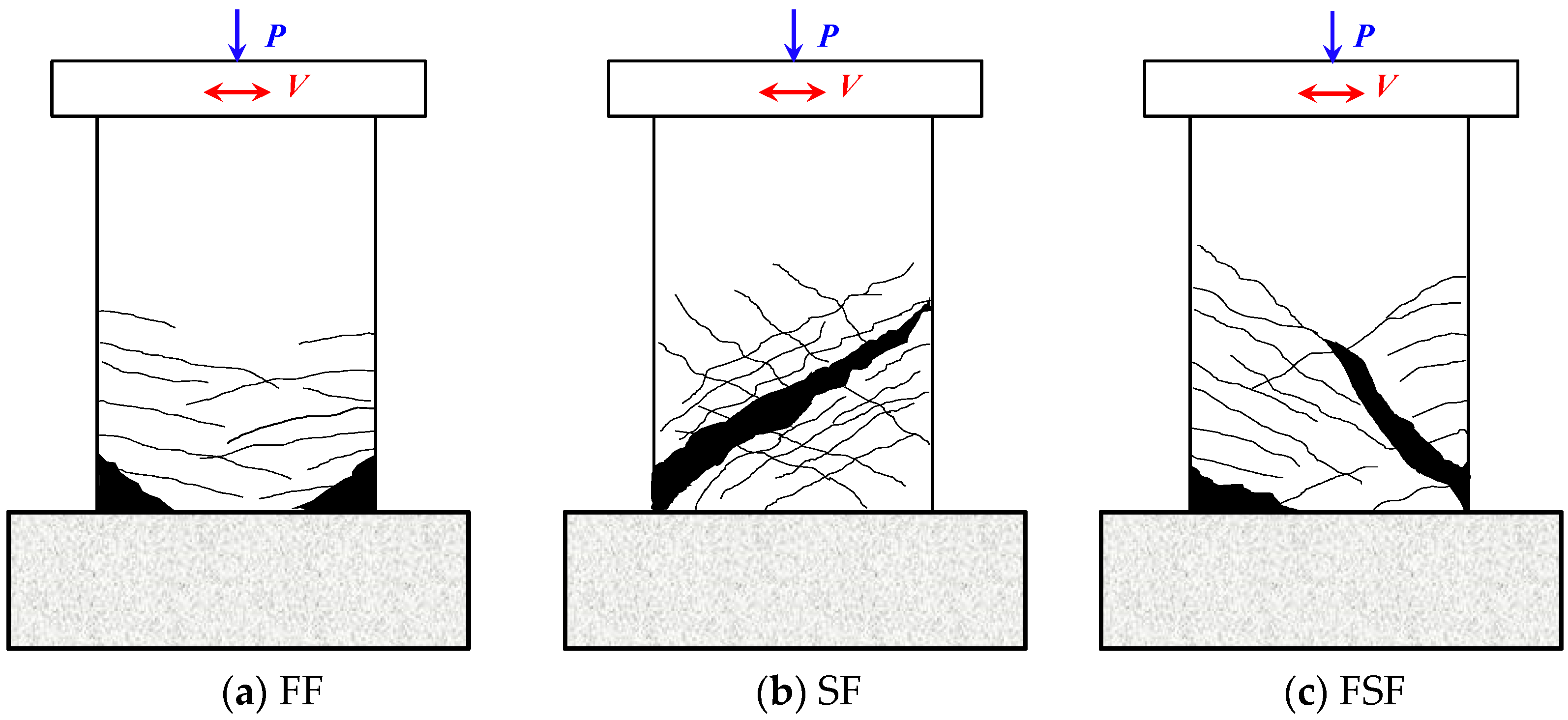
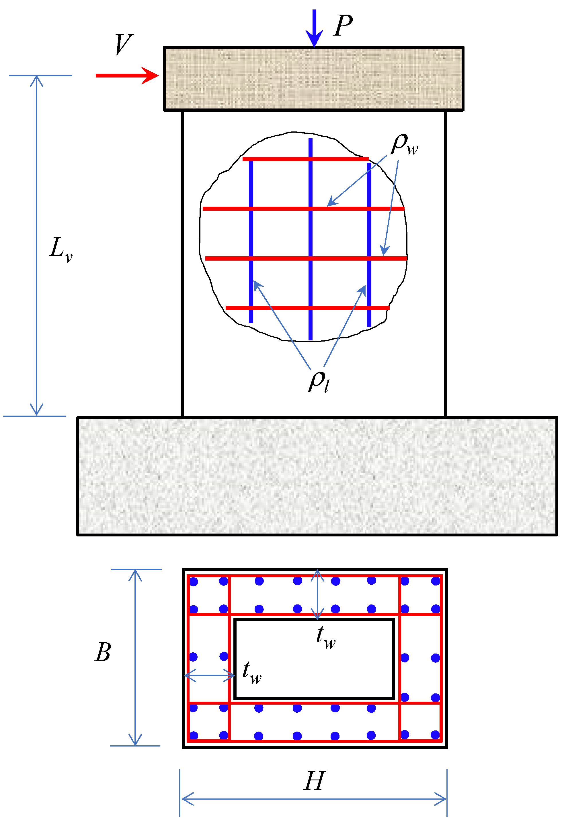
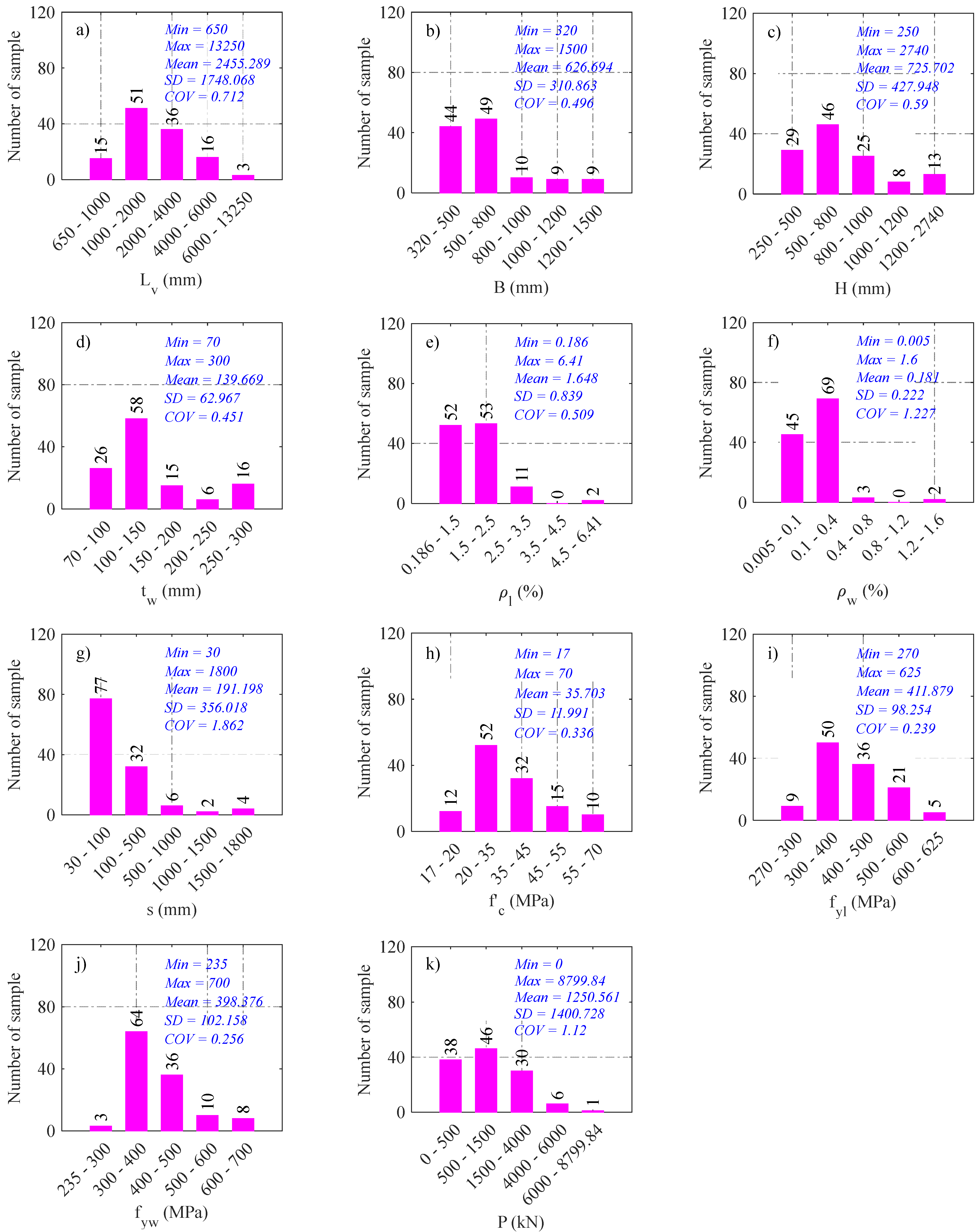
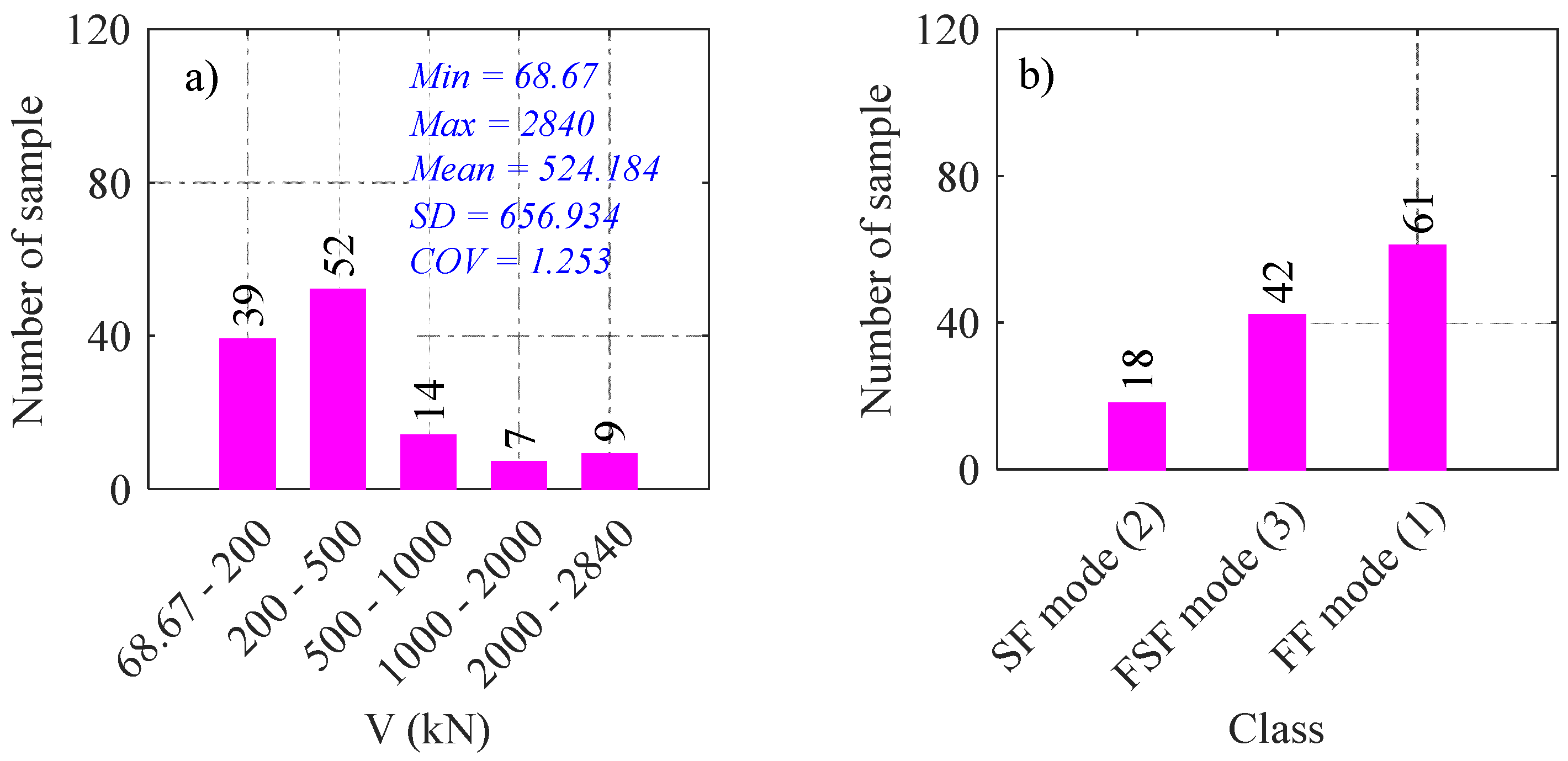
2. Description of Data Collected

This study collects experimental test results of RHRC columns from the literature [1,2,5,12,13,29,30,43,44,45,46,47,48,49] to develop ML models. It should be noted that all experimental samples were published in scientific journals and conference proceedings from 1983 to 2022. The maximum strength values of experimental RC columns are selected as the output values of the database. Moreover, failure modes were emphasized in those experiments. Meanwhile, all eleven design parameters of hollow columns are used for input parameters of the database. Based on the previous studies [6,39,41,50,51], the factors affecting the failure modes and shear strength of RC members can be grouped as geometric dimensions, reinforcing bar details, and material properties. The structural configuration includes the column height (${\mathrm{L}}_{\mathrm{v}}$), the cross-section width ($\mathrm{B}$), the cross-section length ($\mathrm{H}$), and the wall thickness (${\mathrm{t}}_{\mathrm{w}}$). In the case of the reinforcing bar details, the longitudinal reinforcing bar ratio (${\mathsf{\rho }}_{\mathrm{l}}$), the transversal reinforcement ratio (${\mathsf{\rho }}_{\mathrm{w}}$), and the spacing of transversal reinforcements ($\mathrm{s}$) are included. And for the level of material properties, the yield strength of the longitudinal (${\mathrm{f}}_{\mathrm{y}\mathrm{l}}$), the yield strength of the transversal (${\mathrm{f}}_{\mathrm{y}\mathrm{w}}$), and the compressive strength of concrete (${\mathrm{f}}_{\mathrm{c}}^{\prime }$) are crucial. Moreover, the axial load ($\mathrm{P}$) also affects the failure modes and shear strength of RC columns. Therefore, these parameters are collected and considered input variables in this study.

Before constructing the ML models, it is essential to perform comprehensive data analysis. Exploratory data analysis uses statistics and graphs to help recognize trends and examine the consistency and irregularity of the data. In our study, the exploratory data analysis has been completed before moving on to developing ML models. Therefore, the unwanted and incomplete information data points are removed from the database.

It is noted that outlier data points are unusually close together or significantly different from the rest of the dataset. Outliers can reduce the performance of the ML models. However, there is a point of diminishing returns where adding more data may not improve the model performance significantly. In addition, removing outliers can result in losing many data points and information and reducing the data size. As a result, the model’s generalizability is lessened. Notably, some advanced ML models (i.e., XGB) are not affected by outliers. Therefore, only the extreme outliers have been removed from the database. Accordingly, 121 experimental results are retained and used to develop the ML in this study.

Figure 2 schematically shows the configurations and reinforcement properties of RHRC columns. The frequency histograms and statistical properties of input parameters, shear strength, and failure modes of the database are shown in Figure 3 and Figure 4. It should be noted that there are 61, 42, and 18 column samples failed with FF, FSF, and SF, respectively.

3. Overview of ML and Optimization Algorithms

This study uses eight efficient ML algorithms, including SVM, MLP, KNN, DT, RF, GB, AGB, and XGB, for classifying the FMs and predicting the shear strength of RHRC columns. The ML algorithms used in this study can be used for classification and regression problems. They were implemented in the Scikit-learn package [52]. Commonly, the outputs of classification problems are discrete labels, while those of regression problems are continuous values. The following section will briefly introduce eight ML algorithms, while the details of these algorithms have been presented in the previous studies.

3.1. Support Vector Machine

SVM uses statistical learning theory to minimize both the empirical risk and the confidence interval and achieve a good generalization capability. SVM is a highly efficient and robust algorithm for regression and classification problems [53]. The basic idea behind the SVM algorithm is to map the original datasets from the input space to a high- or infinite-dimensional feature space to simplify the problems. To minimize the model complexity and prediction error, SVM uses kernel tricks to build expert knowledge about a problem [54].

3.2. Multi-Layer Perceptron

MLP is a particular class of deep neural network algorithms [55]. The MLP structure consists of an input layer, hidden layer(s), and an output layer. The nodes in the layers are interconnected and have associated thresholds and weights. The training process involves assigning values to these weights. The nodes’ weights are constantly updated to reduce the difference between the predicted and target values.

3.3. K-Nearest Neighbors

KNN locates the $k$-nearest data points in the training set to the point where a target value is missing and applies the approximate value of the identified datasets to it [56]. It has no assumptions about the data distribution. Thus, it is efficient for extensive amounts of training data.

3.4. Decision Tree

The DT model is a simple yet powerful ML algorithm that is commonly used for both classification and regression tasks. It is a tree-like structure, where each internal node represents a feature or attribute, each branch represents a decision based on that feature, and each leaf node represents the outcome or prediction [57]. When training a DT model, the algorithm learns to create the tree by splitting the data based on the features that best separate the classes or explain the target variable. The objective is to minimize the impurity or maximize the information gain at each split, so that the resulting tree can effectively classify or predict the target variable. Once the DT is trained, making predictions is straightforward. The training process starts at the root node by evaluating the feature values and following the corresponding branches until reaching a leaf node. The prediction at that leaf node becomes the final output.

3.5. Random Forest

RF is a popular ML algorithm used for both classification and regression tasks. It is a versatile and powerful model that combines multiple decision trees to make predictions [58]. Random forest would create an ensemble of DTs, in which each tree is trained on different subsets of the data and different subsets of the features. This randomness adds diversity to the individual trees. During prediction, each tree in the forest independently makes its own prediction, and then the final prediction is determined by voting or averaging the predictions of all the trees. This ensemble approach helps to reduce overfitting and improve the accuracy and generalization of the model.

3.6. Boosting Algorithm

The boosting method is an ensemble algorithm that establishes the same structure for all learners trained sequentially [59]. Herein, AGB, GB, and XGB are the boosting algorithms that develop a strong learner based on a set of weak learners. The XGB algorithm enhances the GB algorithm with the objective function that adds a regularization parameter to deal with the overfitting or underfitting problems and reduce model complexity.

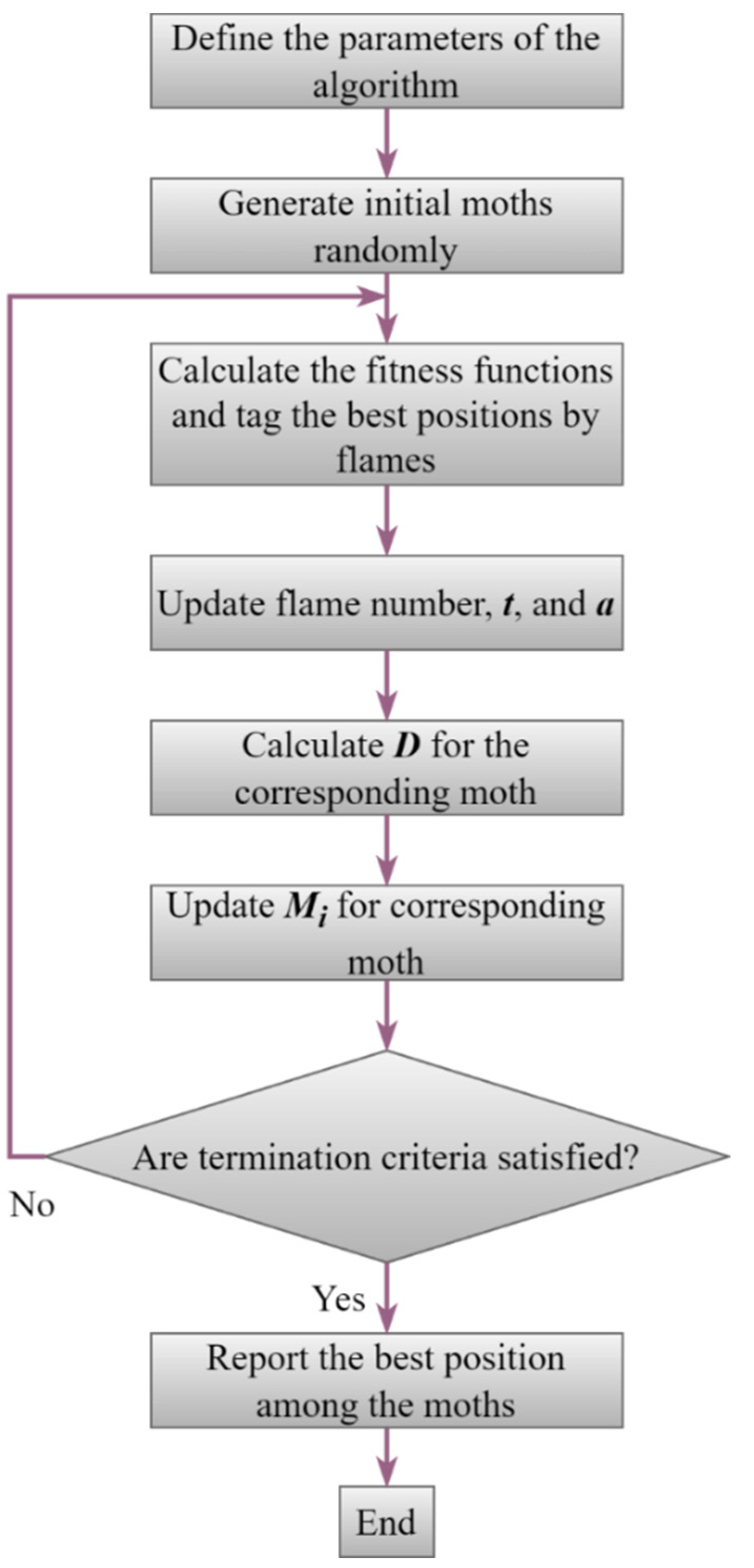
3.7. Moth-Flame Optimization Algorithm

The moth-flame optimization (MFO) algorithm is a nature-inspired optimization algorithm that is inspired by the behavior of moths attracted to a flame [60]. The MFO algorithm is based on the concept that moths are attracted to light sources, such as flames, and tend to move closer to them. However, as they get closer, they also tend to lose energy due to the heat. MFO mimics the behavior of moths in a three-stage process: initialization, attraction, and updating.

• During the initialization stage, a population of moths is randomly placed in the search space. Each moth is represented by a potential solution to the optimization problem.
• In the attraction stage, moths are attracted to a flame, representing the global best solution found so far. The intensity of the flame is determined by the fitness value of the current best solution. Moths are then attracted to the flame based on their proximity to it, with closer moths having a stronger attraction.
• In the updating stage, moths update their positions based on their current position, the position of the flame, and a randomization factor. This movement promotes exploration of the search space, allowing the moths to potentially find better solutions.

The MFO algorithm continues to iterate through the attraction and updating stages until a stopping criterion is met, such as reaching a maximum number of iterations or finding a satisfactory solution. Below is a brief introduction to MFO’s mathematical formulation.

As a first step, the algorithm creates a matrix to represent the set of moths:

$$\mathrm{M}=\left[\begin{array}{cccc}{\mathrm{m}}_{\mathrm{1,1}}& {\mathrm{m}}_{\mathrm{1,2}}& \dots & {\mathrm{m}}_{1,\mathrm{d}}\\ :& :& \dots & :\\ :& :& \dots & :\\ {\mathrm{m}}_{\mathrm{n},1}& {\mathrm{m}}_{\mathrm{n},2}& ..& {\mathrm{m}}_{\mathrm{n},\mathrm{d}}\end{array}\right]$$

(1)

In the second step, the algorithm expresses the flames in a matrix as follows:

$$\mathrm{F}=\left[\begin{array}{cccc}{\mathrm{F}}_{\mathrm{1,1}}& {\mathrm{F}}_{\mathrm{1,2}}& \dots & {\mathrm{F}}_{1,\mathrm{d}}\\ :& :& \dots & :\\ :& :& \dots & :\\ {\mathrm{F}}_{\mathrm{n},1}& {\mathrm{F}}_{\mathrm{n},2}& ..& {\mathrm{F}}_{\mathrm{n},\mathrm{d}}\end{array}\right]$$

(2)

where $\mathrm{d}$ and $\mathrm{n}$ are the numbers of variables and moths, respectively.

The fitness values are as follows:

$$\mathrm{O}\mathrm{M}=\left[\begin{array}{c}{\mathrm{O}\mathrm{M}}_1\\ :\\ :\\ {\mathrm{O}\mathrm{M}}_{\mathrm{n}}\end{array}\right] \text{and} \mathrm{O}\mathrm{F}=\left[\begin{array}{c}{\mathrm{O}\mathrm{F}}_1\\ :\\ :\\ {\mathrm{O}\mathrm{F}}_{\mathrm{n}}\end{array}\right]$$

(3)

In the MFO algorithm, each moth seeks around a flame to update its position using the equation below:

$${\mathrm{M}}_{\mathrm{i}}=\mathrm{S}\left({\mathrm{M}}_{\mathrm{i}},{\mathrm{F}}_{\mathrm{j}}\right)={\mathrm{D}}_{\mathrm{i}}·{\mathrm{e}}^{\mathrm{b}\mathrm{t}}·\cos \left(2\mathsf{\pi }\mathrm{t}\right)+{\mathrm{F}}_{\mathrm{j}}$$

(4)

$$\mathrm{t}=\left(\mathrm{a}-1\right)\times \mathrm{r}\mathrm{a}\mathrm{n}\mathrm{d}\left(\right)+1$$

(5)

$$\mathrm{a}=-1+\mathrm{I}\mathrm{t}\mathrm{e}\mathrm{r}\times \left(\right(-1)/\mathrm{M}\mathrm{a}\mathrm{x}\mathrm{I}\mathrm{t}\mathrm{e}\mathrm{r})$$

(6)

where ${\mathrm{M}}_{\mathrm{i}}$ is the ${\mathrm{i}}^{}\mathrm{th}$ moth, ${\mathrm{F}}_{\mathrm{j}}$ is the jth flame, $\mathrm{S}$ is the spiral function, $\mathrm{b}$ is a constant, and ${\mathrm{D}}_{\mathrm{i}}$ is the distance of the ${\mathrm{i}}^{}\mathrm{th}$ moth from the $\mathrm{j}\mathrm{t}\mathrm{h}$ flame. ${\mathrm{D}}_{\mathrm{i}}$ is calculated as below:

$${\mathrm{D}}_{\mathrm{i}}=|{\mathrm{F}}_{\mathrm{j}}-{\mathrm{M}}_{\mathrm{i}}|$$

(7)

The flames’ number is calculated as follows:

$$\mathrm{f}\mathrm{l}\mathrm{a}\mathrm{m}\mathrm{e}\_\mathrm{n}\mathrm{o}=\mathrm{r}\mathrm{o}\mathrm{u}\mathrm{n}\mathrm{d}\left(\mathrm{N}-\mathrm{I}\mathrm{t}\mathrm{e}\mathrm{r}\ast \frac{(\mathrm{N}-1)}{\mathrm{M}\mathrm{a}\mathrm{x}\mathrm{I}\mathrm{t}\mathrm{e}\mathrm{r}}\right)$$

(8)

where $\mathrm{N}$, $\mathrm{I}\mathrm{t}\mathrm{e}\mathrm{r}$, and $\mathrm{M}\mathrm{a}\mathrm{x}\mathrm{I}\mathrm{t}\mathrm{e}\mathrm{r}$ are the maximum numbers of flames, the current number of iterations, and the maximum iterations, respectively. Figure 5 demonstrates the flowchart of the MFO algorithm. The detail of the MFO algorithm can be found in Mirjalili [60].

3.8. Synthetic Minority Over-Sampling Technique

Figure 4 shows that the failure modes are highly imbalanced for the classification task. The database contains 61, 42, and 18 samples for FF, FSF, and SF modes, respectively. Therefore, this issue can adversely affect the accuracy of ML algorithms. In this study, the SMOTE [61] is used to overcome this drawback. Accordingly, the SMOTE increases the number of small classes to the largest one. However, the SMOTE algorithm remains the same for each class’s statistics and region. The SMOTE has proven successful for the class imbalance problem. After adopting the SMOTE technique, the database comprises 61, 61, and 61 samples for FF, FSF, and SF modes, respectively. This synthetic database can be found in Supplementary Materials. Following typical steps are required to perform the SMOTE.

(1)

Identify the imbalanced dataset: Determine which class in your dataset is the minority class that needs to be oversampled.

(2)

Import necessary libraries: Depending on the programming language used, the required libraries or packages for SMOTE implementation are imported. In this study, we adopt the scikit-learn library for Python.

(3)

Split the dataset: Divide the dataset into features (X) and the corresponding class labels (Y).

(4)

Apply SMOTE: the SMOTE algorithm is employed to generate synthetic samples for the minority class. This involves the following sub-steps:

• Identify the minority class samples: Separate the minority class samples from the majority class samples.
• Determine the number of synthetic samples to generate: Decide on the desired ratio of minority to majority class samples after oversampling. This ratio can be adjusted based on the specific problem and dataset.
• Compute the k-nearest neighbors: For each minority class sample, identify its k-nearest neighbors from the minority class samples.
• Generate synthetic samples: Randomly select one of the k-nearest neighbors and create a new synthetic sample along the line connecting the two points. Repeat this process for the desired number of synthetic samples.

(5)

Combine the original and synthetic samples: Combine the original minority class samples with the newly generated synthetic samples to create a balanced dataset.

4. Performance Metrics

Performance metrics are essential in evaluating ML models since they provide values to objectively measure and analyze the performance of the predictive model. This helps users understand the strengths and weaknesses of the model and identify areas for improvement. Performance metrics are also indicators for comparing different models and determining which one is the most effective for a specific task.

Furthermore, performance metrics work by analyzing the output of an ML model against a known set of data (i.e., experimental data). This is required to measure the accuracy, precision, and recall of the model, among other metrics. The results are then compared to a desired level of performance, and any discrepancies can be addressed through further training or adjusting the model’s parameters.

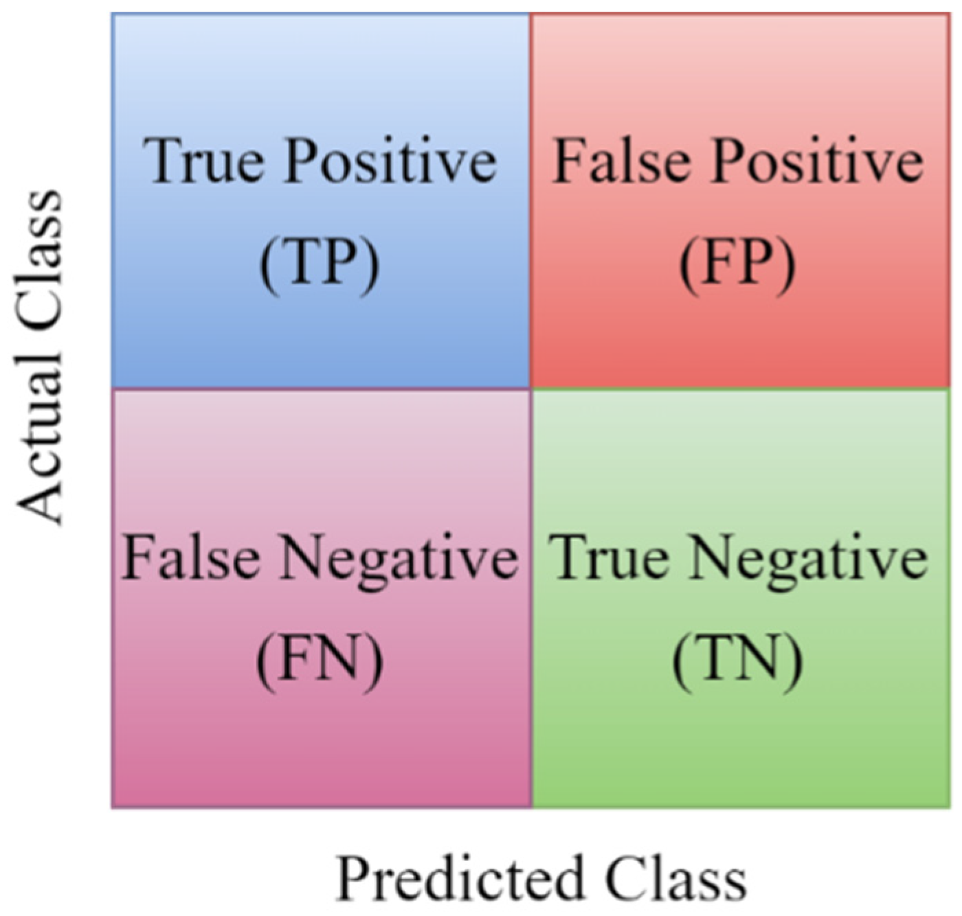
4.1. Classification Metrics

To evaluate the classification ML models’ efficiency, several metrics, such as accuracy, recall, precision, f1-score, and area under the curve (AUC) of the receiver-operating characteristic (ROC) curve, are used in this study. These metrics are calculated based on the confusion matrix, as shown in Figure 6.

In the confusion matrix, the diagonal values correspond to the correct prediction failure modes; the off-diagonal values correspond to the failure modes not correctly predicted. Each row denotes an actual class, while each column indicates a predicted class. The accuracy, recall, precision, and f1-score are expressed as:

$$\mathrm{A}\mathrm{c}\mathrm{c}\mathrm{u}\mathrm{a}\mathrm{c}\mathrm{y}=\frac{\mathrm{T}\mathrm{P}+\mathrm{T}\mathrm{N}}{\mathrm{T}\mathrm{P}+\mathrm{T}\mathrm{N}+\mathrm{F}\mathrm{P}+\mathrm{F}\mathrm{N}}$$

(9)

$$\mathrm{P}\mathrm{r}\mathrm{e}\mathrm{c}\mathrm{i}\mathrm{s}\mathrm{i}\mathrm{o}\mathrm{n}=\frac{\mathrm{T}\mathrm{P}}{\mathrm{T}\mathrm{P}+\mathrm{F}\mathrm{P}}$$

(10)

$$\mathrm{R}\mathrm{e}\mathrm{c}\mathrm{a}\mathrm{l}\mathrm{l}=\frac{\mathrm{T}\mathrm{P}}{\mathrm{T}\mathrm{P}+\mathrm{F}\mathrm{N}}$$

(11)

$$\mathrm{f}1\text{-}\mathrm{s}\mathrm{c}\mathrm{o}\mathrm{r}\mathrm{e}=2\times \frac{\mathrm{P}\mathrm{r}\mathrm{e}\mathrm{c}\mathrm{i}\mathrm{s}\mathrm{i}\mathrm{o}\mathrm{n}\times \mathrm{R}\mathrm{e}\mathrm{c}\mathrm{a}\mathrm{l}\mathrm{l}}{\mathrm{P}\mathrm{r}\mathrm{e}\mathrm{c}\mathrm{i}\mathrm{s}\mathrm{i}\mathrm{o}\mathrm{n}+\mathrm{R}\mathrm{e}\mathrm{c}\mathrm{a}\mathrm{l}\mathrm{l}}$$

(12)

It is noted that the higher the accuracy, recall, precision, and f1-score, the more efficient performance of ML models.

4.2. Regression Metrics

This study uses three prevalent metrics, including goodness of fit (${\mathrm{R}}^2$), root mean squared error (RMSE), and mean absolute error (MAE), to evaluate the performance of the regression ML models.

$${\mathrm{R}}^2=1-\frac{\sum _{\mathrm{i}=1}^{\mathrm{n}}{({\mathrm{y}}_{\mathrm{i}}-{\widehat{\mathrm{y}}}_{\mathrm{i}})}^2}{\sum _{\mathrm{i}=1}^{\mathrm{n}}{({\mathrm{y}}_{\mathrm{i}}-\overline{\mathrm{y}})}^2}$$

(13)

$$\mathrm{A}10=\frac{\mathrm{n}10}{\mathrm{n}}$$

(14)

$$\mathrm{R}\mathrm{M}\mathrm{S}\mathrm{E}=\sqrt{\frac{1}{\mathrm{n}}\sum _{\mathrm{i}=1}^{\mathrm{n}}{({\mathrm{y}}_{\mathrm{i}}-{\widehat{\mathrm{y}}}_{\mathrm{i}})}^2}$$

(15)

$$\mathrm{M}\mathrm{A}\mathrm{E}=\frac{1}{\mathrm{n}}\sum _{i=1}^n|y_i-{\widehat{y}}_i|$$

(16)

where ${\mathrm{y}}_{\mathrm{i}}$ is the target shear strength, ${\widehat{y}}_i$ is the predicted shear strength, $\overline{y}$ is the average value of target shear strength, $\mathrm{n}10$ is the number of samples with the value of the ratio of experimental value to a predicted value falling between 0.90 and 1.10, and $\mathrm{n}$ is the number of data points.

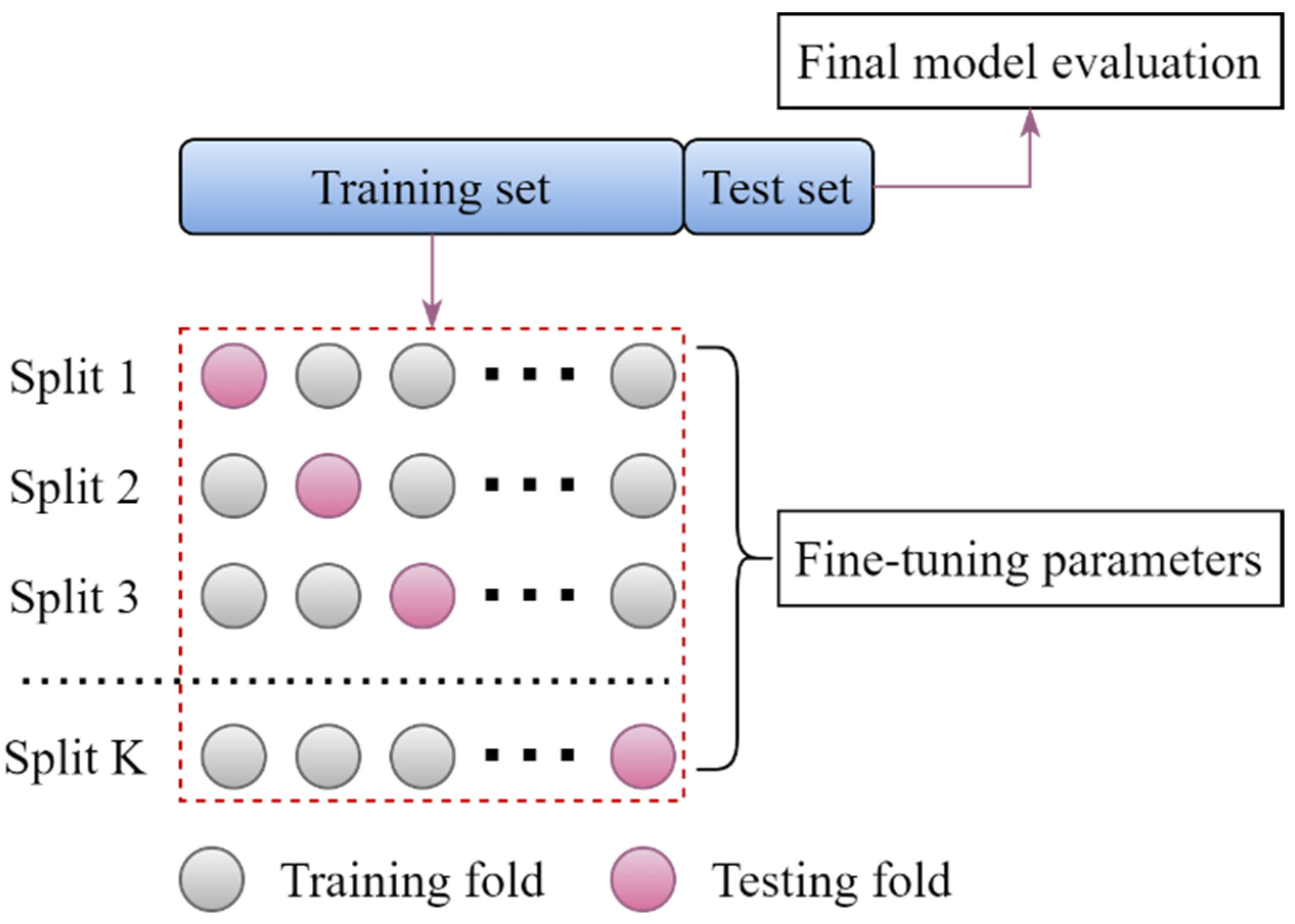
4.3. K-Fold Cross-Validation

In this study, K-fold CV is used to avoid overfitting and get the ML models’ generalization performance on the unseen data. The process of this technique is presented in Figure 7. The K-fold CV divides the training set into $\mathrm{K}$ subsets of the same size. Accordingly, training folds consist of $\mathrm{K}-1$ subsets, while testing folds consist of the remaining subset. Thus, the ML model is trained $\mathrm{K}$ times. Performance of the model is measured using average $\mathrm{K}$ folds. Herein, the stratified five-fold CV is used for classification ML models, while the standard five-fold CV is used for regression ML models.

5. Development of ML Models

Figure 8 shows the flowchart for developing the classification and regression ML models used in this study. The following section introduces the detailed descriptions of the procedure.

5.1. Input and Output Variables

In this study, ${\mathrm{L}}_{\mathrm{v}}$, $\mathrm{B}$, $\mathrm{H}$, ${\mathrm{t}}_{\mathrm{w}}$, ${\mathsf{\rho }}_{\mathrm{l}}$, ${\mathsf{\rho }}_{\mathrm{w}}$, $\mathrm{s}$, ${\mathrm{f}}_{\mathrm{c}}^{\prime }$, ${\mathrm{f}}_{\mathrm{y}\mathrm{l}}$, ${\mathrm{f}}_{\mathrm{y}\mathrm{w}}$, and $\mathrm{P}$ are used as input variables to classify the failure modes (i.e., FF, SF, and FSF), and predict the shear strength of RHRC columns.

This study uses z-normalization for input variables to develop the ML models since raw data extracted from various sources have different units and ranges. This method converts the mean of each input variable to around zero and the standard deviation to about one and retains the distribution of values. The z-normalization is expressed as:

$${\mathrm{z}}_{\mathrm{I},\mathrm{j}}=\frac{I-{\overline{\mathrm{x}}}_{\mathrm{j}}}{{\mathsf{\sigma }}_{\mathrm{j}}}$$

(17)

where ${\mathrm{x}}_{\mathrm{i},\mathrm{j}}$ Is the $\mathrm{j}\mathrm{t}\mathrm{h}$ input variable of $\mathrm{i}\mathrm{t}\mathrm{h}$ data sample, ${\mathrm{z}}_{\mathrm{i},\mathrm{j}}$ is the standardized value of ${\mathrm{x}}_{\mathrm{i},\mathrm{j}}$, ${\overline{\mathrm{x}}}_{\mathrm{j}}$ is the mean of $\mathrm{j}\mathrm{t}\mathrm{h}$ input variables, and ${\mathsf{\sigma }}_{\mathrm{j}}$ is the standard deviation of $\mathrm{j}\mathrm{t}\mathrm{h}$ input variables.

5.2. Hyperparameter Tuning

Parameters and hyperparameters are fundamental to ML algorithms. Parameters are internal configuration variables whose values can be inferred from the dataset. Meanwhile, hyperparameters are used to regulate how the model learns [62,63]. The hyperparameter value can be set by default in the ML package or adjusted by the user. However, ML models with default parameters have the major disadvantage of overfitting or underfitting because they introduce bias and variance [64,65,66]. Therefore, hyperparameter selection becomes an important criterion in every ML model. Model prediction can be significantly enhanced by selecting precise hyperparameters [65,67,68]. However, manually choosing all possible hyperparameter values for each ML model is time-consuming and impractical. Therefore, this study utilizes the MFO algorithm for tuning the hyperparameters of the ML models.

The step-by-step procedure for constructing the hybrid ML models is shown in Figure 8. Firstly, the data samples are arbitrary split into training and test sets. Models are established from the training set to choose the best values of hyperparameters; meanwhile, the test set is used to see how the models perform. In this study, eight training ratios (i.e., 0.55, 0.60, 0.65, 0.70, 0.75, 0.80, 0.85, and 0.90) and corresponding test ratios (i.e., 0.45, 0.40, 0.35, 0.30, 0.25, 0.20, 0.15, and 0.10), respectively, are used to investigate the effect of training and test data partitions. Additionally, six population sizes (50, 100,150, 200, 250, and 300) in the MFO algorithm are considered. This study utilizes a five-fold CV for the training dataset. The process is repeated five times via the MFO algorithm, and the test folds are averaged to establish a prediction model. The fitness functions are the average f1-score of five testing folds in the classification models and the average MAE of five testing folds in the regression ones. The primary hyperparameters and their ranges for the classification and regression ML models are presented in

Table 1. Hyperparameters of classification ML algorithms.

Model	No.	Hyperparameters	Range	Optimal Value
SVM	1	C	(0.01, 1.0)	0.968473
	2	degree	(1, 5)	2
	3	tol	(0.01, 1.0)	0.056104
MLP	1	alpha	(0.01, 1.0)	0.711483
	2	batch_size	(1, 100)	26
	3	hidden_layer_sizes	(1, 100)	10
	4	momentum	(0.01, 1.0)	0.155035
KNN	1	leaf_size	(1, 100)	64
	2	n_neighbors	(1, 50)	1
	3	p	(1, 2)	1
DT	1	max_depth	(1, 100)	79
	2	min_samples_leaf	(1, 10)	5
	3	min_samples_split	(1, 10)	8
	4	min_weight_fraction_leaf	(0.1, 1.0)	0.036477
RF	1	max_depth	(1, 100)	17
	2	min_samples_leaf	(1, 10)	5
	3	min_samples_split	(1, 10)	3
	4	n_estimators	(5, 1000)	23
AGB	1	learning_rate	(0.01, 1.0)	0.629896
	2	n_estimators	(5, 1000)	165
GB	1	learning_rate	(0.01, 1.0)	0.681775
	5	n_estimators	(5, 1000)	689
	3	min_samples_split	(1, 10)	3
	2	min_samples_leaf	(1, 10)	9
	1	max_depth	(1, 100)	16
XGB	1	learning_rate	(0.01, 1.0)	0.557980
	2	max_depth	(1, 100)	8
	3	n_estimators	(5, 1000)	921

and

Table 2. Hyperparameters of regression ML algorithms.

Model	No.	Hyperparameters	Range	Optimal Value
SVM	1	C	(0.01, 1.0)	0.999992
	2	gama	(0.01, 1.0)	0.086386
	3	degree	(1, 5)	2
	4	epsilon	(0.01, 1.0)	0.602402
MLP	1	alpha	(0.01, 1.0)	0.541640
	2	batch_size	(1, 100)	4
	3	hidden_layer_sizes	(1, 100)	66
	4	momentum	(0.01, 1.0)	0.752071
KNN	1	leaf_size	(1, 100)	27
	2	n_neighbors	(1, 50)	1
	3	p	(1, 2)	2
DT	1	max_depth	(1, 100)	53
	2	min_samples_leaf	(1, 10)	1
	3	min_samples_split	(1, 10)	4
	4	min_weight_fraction_leaf	(0.1, 1.0)	0.1
RF	1	max_depth	(1, 100)	100
	2	min_samples_leaf	(1, 10)	1
	3	min_samples_split	(1, 10)	2
	4	n_estimators	(5, 1000)	649
AGB	1	learning_rate	(0.01, 1.0)	0.543211
	2	n_estimators	(5, 1000)	452
GB	1	learning_rate	(0.01, 1.0)	0.343455
	2	n_estimators	(5, 1000)	204
	3	subsample	(0.1, 1.0)	0.916063
	4	max_depth	(1, 100)	4
	5	alpha	(0.1, 1.0)	0.468587
XGB	1	learning_rate	(0.01, 1.0)	0.745099
	2	max_depth	(1, 100)	55
	3	n_estimators	(5, 1000)	5

. Detailed descriptions of the hyperparameters were presented in the Scikit-learn package [52].

6. Results and Discussions

6.1. Choosing the Best Regression and Classification Models

Data splitting plays a crucial role in ML models’ performance assessment [68]. For this purpose, eight ratios (i.e., 0.55–0.45, 0.60–0.40, 0.65–0.35, 0.70–0.30, 0.75–0.25, 0.80–0.20, 0.85–0.15, and 0.90–0.10 for training and test set, respectively) and six population sizes (i.e., 50, 100, 150, 200, 250, and 300) are investigated in this section. Statistical metrics are employed for evaluating the performance of ML models. The classification ML models perform better when the measuring paramenters (i.e., accuracy, precision, recall, and f1-score) are high. Moreover, the regression ML models perform better when the R² and A10 are high. In contrast, the regression ML models perform better when RMSE and MAE are low. It is observed that the ML models’ performance changes according to the variation of training–test ratios and population sizes.

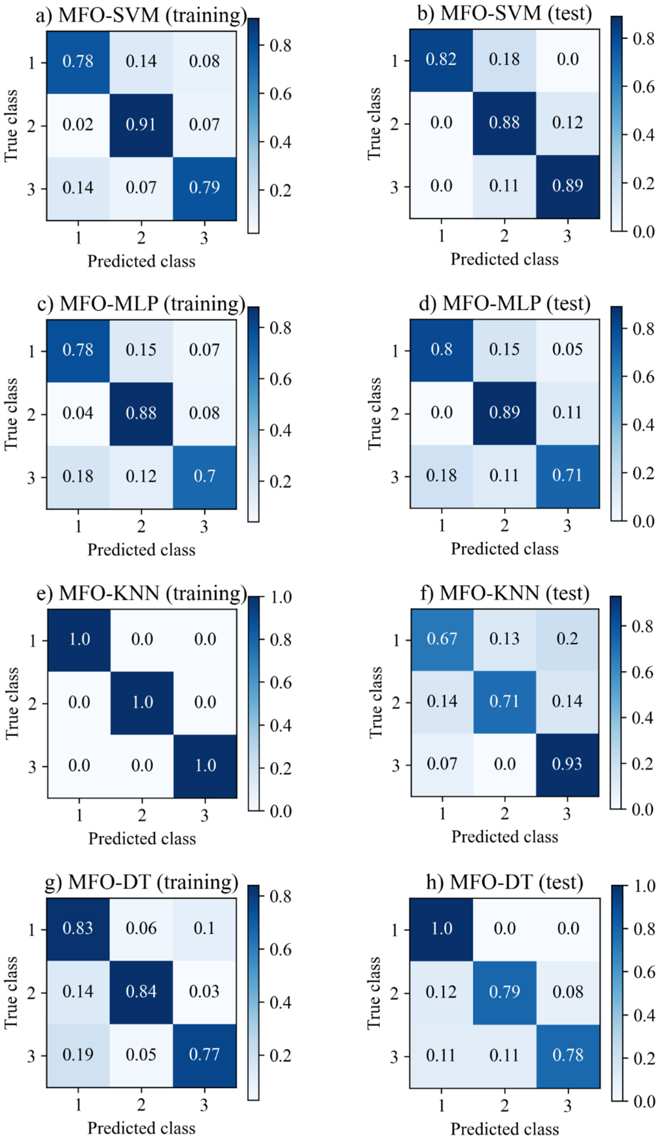
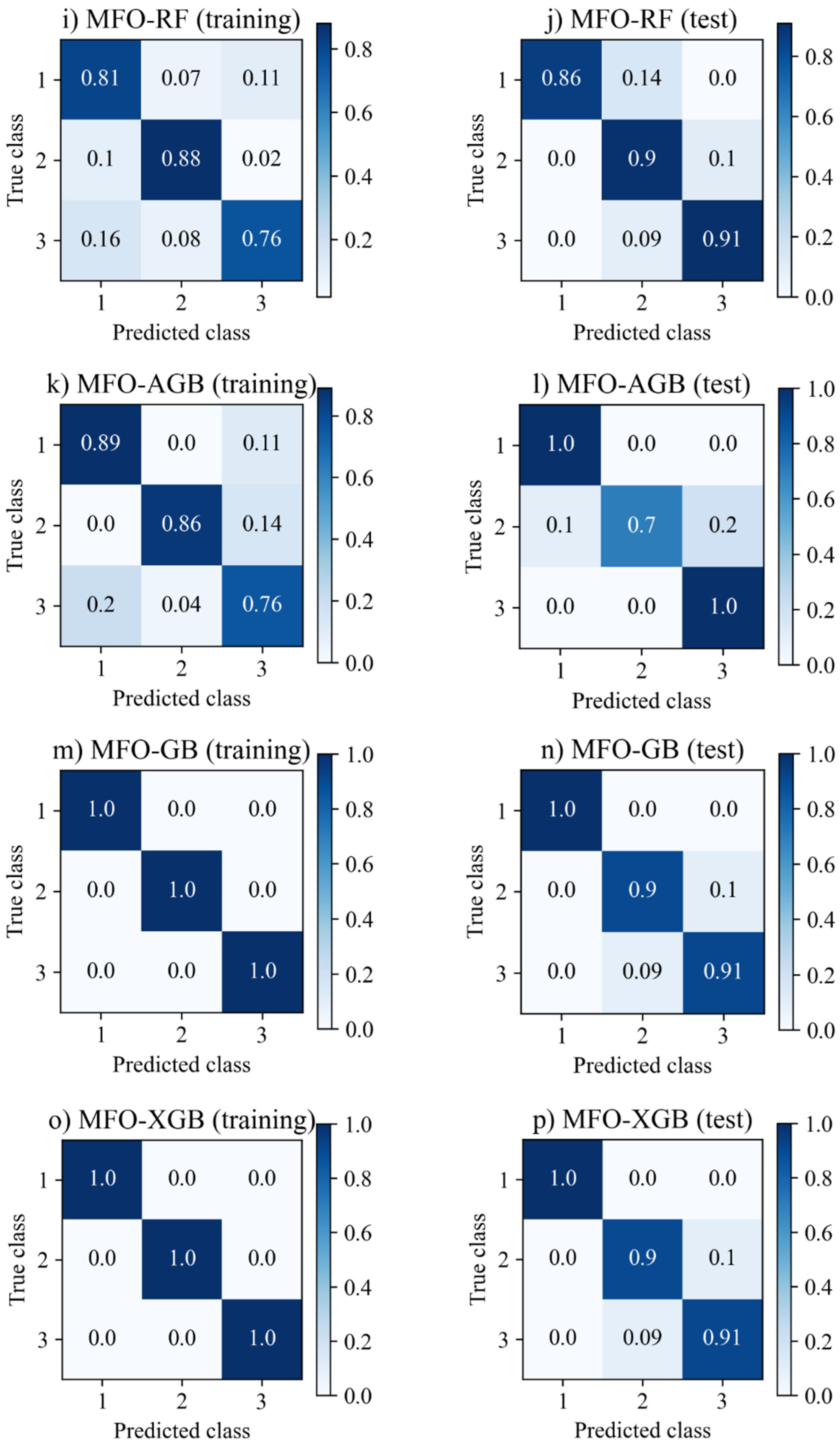
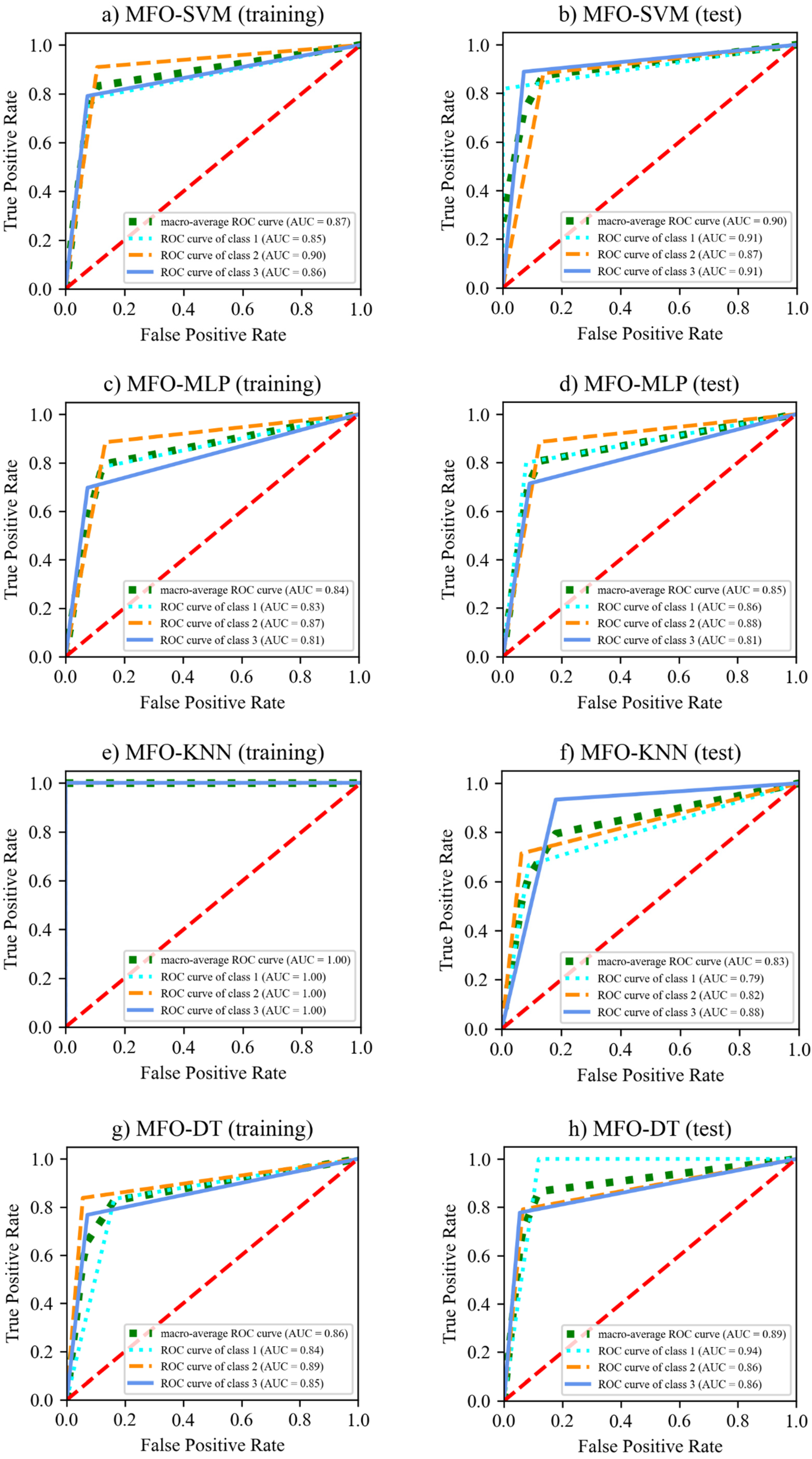
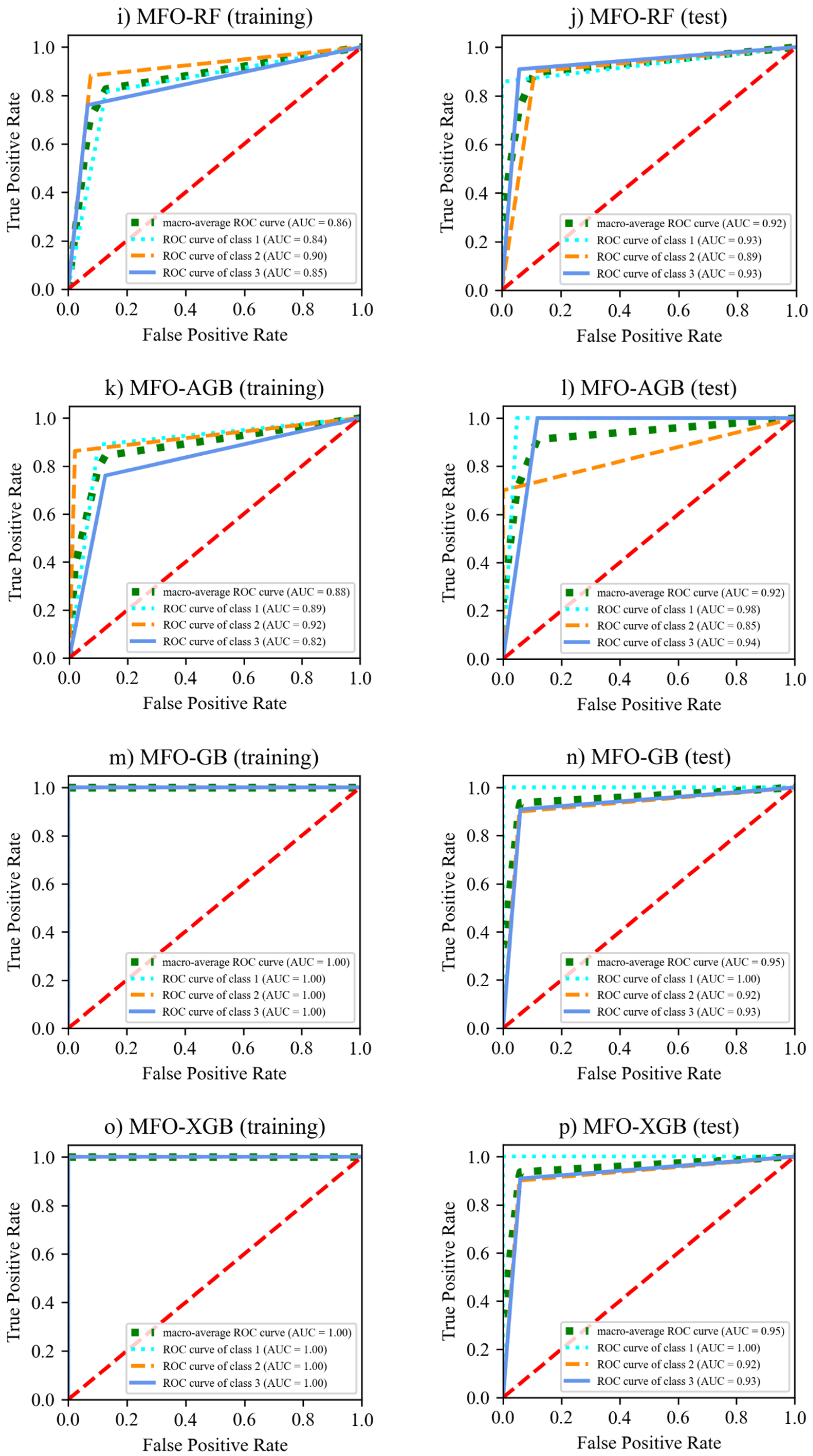
6.2. Performance of ML Models for Failure Modes

The best training–test ratio and population size for the classification MFO-SVM, MFO-MLP, MFO-KNN, MFO-DT, MFO-RF, MFO-AB, MFO-GB, and MFO-XGB models are (75–25, 50), (55–45, 50), (80–20, 150), (70–30, 250), (85–15, 150), (85–15, 150), (85–15, 50), and (85–15, 50), respectively. Optimal hyperparameter values of the classification and regression ML models are listed in Table 1 and Table 2.

Figure 9 presents the classifying performance of eight data-driven models using confusion matrices in the normalized form (the non-normalized form can be found in Supplementary Materials). The accuracy, recall, precision, and f1-score metrics of the training and test sets are calculated from the confusion matrix and used to evaluate the performance of the classification ML models, as shown in

Table 3. Performance of classification ML models.

Model	Training Set				Test Set
	Accuracy	Precision	Recall	F1-Score	Accuracy	Precision	Recall	F1-Score
MFO-SVM	0.825	0.827	0.825	0.824	0.870	0.879	0.870	0.871
MFO-MLP	0.780	0.789	0.780	0.780	0.807	0.807	0.807	0.806
MFO-KNN	1.0	1.0	1.0	1.0	0.784	0.788	0.784	0.779
MFO-DT	0.812	0.816	0.812	0.813	0.836	0.852	0.836	0.836
MFO-RF	0.819	0.821	0.819	0.819	0.893	0.899	0.893	0.894
MFO-AGB	0.839	0.843	0.839	0.840	0.893	0.908	0.893	0.888
MFO-GB	1.0	1.0	1.0	1.0	0.925	0.925	0.925	0.925
MFO-XGB	1.0	1.0	1.0	1.0	0.929	0.929	0.929	0.929

.

The confusion matrix has three rows and three columns according to three FMs. In the confusion matrix, labels 1, 2, and 3 represent FF, SF, and FSF, respectively. The diagonal cells indicate the correct samples’ prediction, and the off-diagonal numbers are the misclassified samples. Overall, all the ML models perform well with the training set. Since the testing set represents the generalization capability, it is used to evaluate the performance of the ML models. The results show that the MFO-GB and MFO-XGB models are superior to other models. In addition, the MFO-AGB, MFO-RF, MFO-DT, MFO-MLP, and MFO-SVM models also have good accuracy for the test set. Meanwhile, the MFO-KNN model performs worst among the models. In summary, the MFO-XGB model yields the best accuracy in the FM identification of the RHRC columns.

For a better understanding of the model performance, the ROC curve is also used to compare the classification ML models, as shown in Figure 10. In these plots, the x-axis represents the FP rate while the y-axis represents the TP rate. The diagonal red dashed lines indicate random-guess models. The model with higher TP and AUC and lower FP rates is more accurate.

According to these figures, the AUC values of the MFO-SVM, MFO-MLP, MFO-KNN, MFO-DT, MFO-RF, MFO-AGB, MFO-GB, and MFO-XGB models are (0.87, 0.90), (0.84, 0.85), (1.0, 0.83), (0.86, 0.89), (0.86, 0.92), (0.88, 0.92), (1.0, 0.95), and (1.0, 0.95), for the training and test sets, respectively. One can observe that the MFO-GB and MFO-XGB models are better than the other models, since they reach more quickly towards the top left. Overall, these results show that the MFO-XGB model is the most reliable and accurate in classifying the failure modes of the RHRC columns.

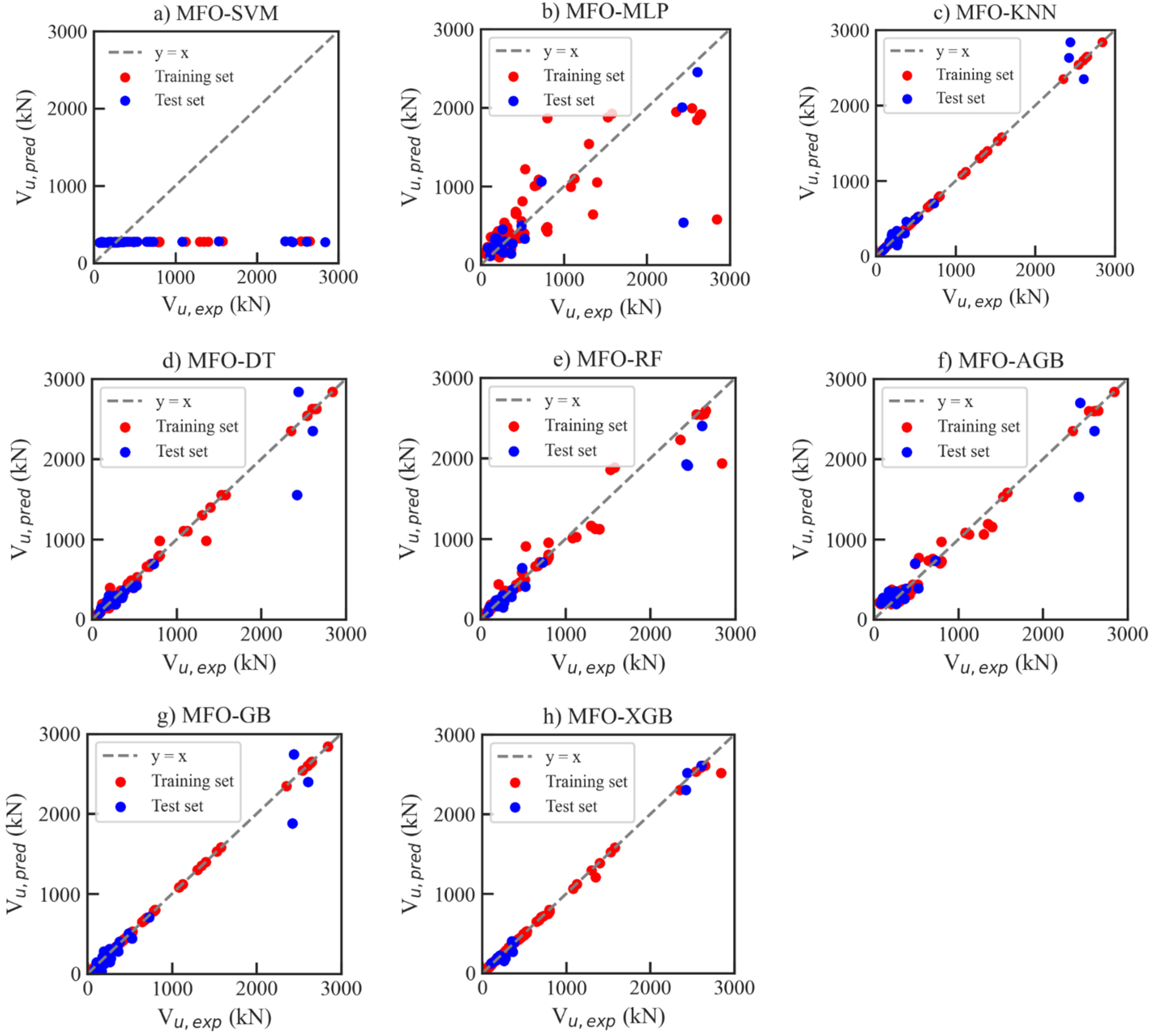
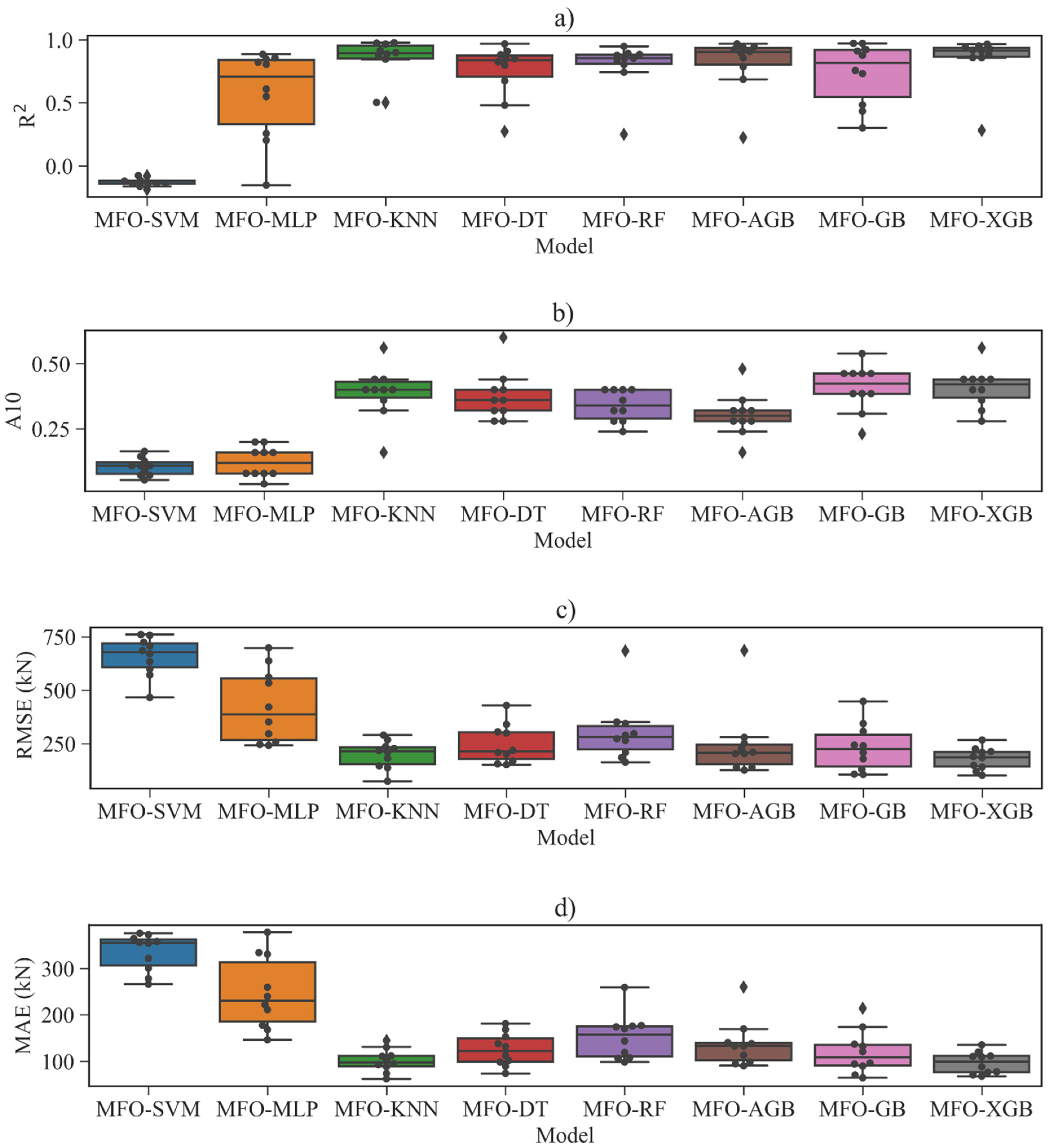
6.3. Performance of ML Models for Shear Strength

The best training–test ratio and population size for the regression MFO-SVM, MFO-MLP, MFO-KNN, MFO-DT, MFO-RF, MFO-AB, MFO-GB, and MFO-XGB models are (55–45, 150), (80–20, 100), (80–20, 50), (80–20, 50), (80–20, 250), (80–20, 50), (80–20, 50), and (90–10, 250), respectively. Optimal hyperparameter values of the classification and regression ML models are listed in Table 1 and Table 2.

Figure 11 and

Table 4. Performance of regression ML models.

Model	Training Set				Test Set
	R2	A10	RMSE (kN)	MAE (kN)	R2	A10	RMSE (kN)	MAE (kN)
MFO-SVM	0.136	0.106	667.668	337.376	0.139	0.145	731.866	367.893
MFO-MLP	0.695	0.188	349.179	192.981	0.675	0.320	416.404	203.310
MFO-KNN	1.0	1.0	0.0	0.0	0.975	0.400	116.123	71.106
MFO-DT	0.992	0.854	55.347	22.437	0.922	0.360	203.606	97.192
MFO-RF	0.962	0.677	123.997	50.529	0.952	0.400	160.101	88.156
MFO-AGB	0.977	0.365	96.286	75.644	0.916	0.360	212.269	120.163
MFO-GB	1.0	1.0	0.008	0.006	0.963	0.488	140.724	79.073
MFO-XGB	0.997	0.944	35.186	10.514	0.996	0.615	62.427	46.027

show the training and test performances of the regression ML models. This figure shows that the MFO-XGB model has the highest potential for estimating the shear strength of RHRC columns when most prediction values are in good agreement with the actual values. The ${\mathrm{R}}^2$, A10, RMSE, and MAE values of the MFO-XGB model for training and test sets are (0.997, 0.996), (0.944, 0.615), (35.186, 62.427) kN, and (10.514, 46.027) kN, respectively. The second-best models are MFO-KNN, MFO-GB, MFO-RF, MFO-DT, and MFO-AGB models. Moreover, the MFO-SVM model presents the worst performance, with the ${\mathrm{R}}^2$ value being lower than 0.2 for the training and test sets. In addition, the RMSE and MAE values of the MFO-SVM model are higher than that of the other models.

Figure 12 show the box-plot of all the metrics of the ML models in the test phases after ten runs. It can be seen again that the MFO-XGB is the best one among ML models. Among the considered ML models, the MFO-XGB model has the highest ${\mathrm{R}}^2$ and A10 values (0.997 and 0.615, respectively) and the smallest RMSE and MAE (62.4 kN and 46 kN, respectively). The second-best model is MFO-KNN with ${\mathrm{R}}^2$, A10, RMSE, and MAE of 0.975, 0.4, 116 kN and 71 kN, respectively. The excellent performance of MFO-XGB obtained may be due to the combination of the powerful XGB and the strong optimization algorithm like MFO [62]. This implies that MFO-XGB is the optimal model in predicting the shear strength of RHRC columns.

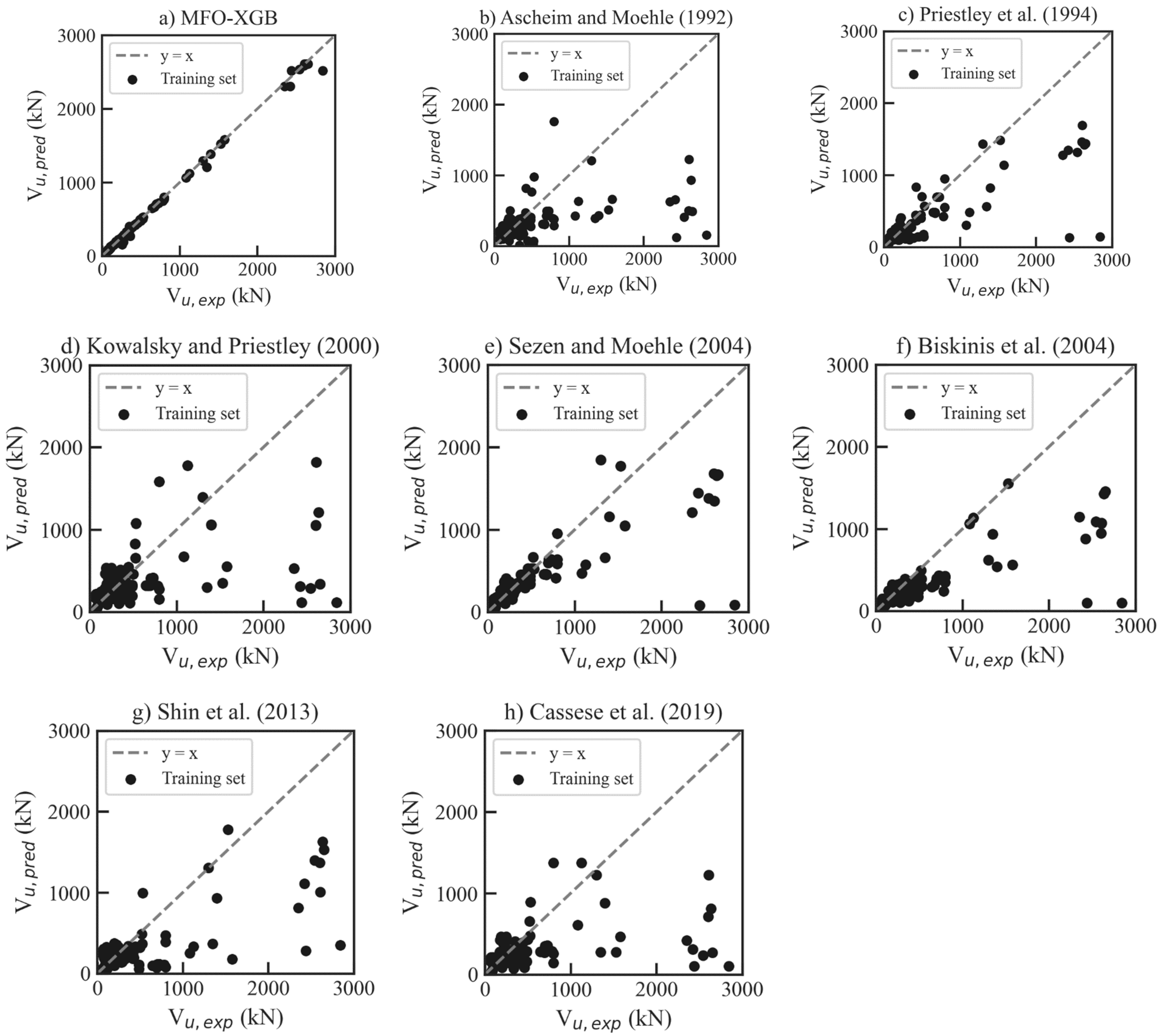
6.4. Comparison of Shear Strength between Different Predictive Models

Previous studies mainly developed formulas for estimating the shear strength of solid RC columns [4,22,23,24,25,26]. Those equations also have been applied to RHRC columns. However, hollow columns may behave differently from the solid ones when subjected to lateral loads. So far, only one specific equation for predicting the shear strength of RHRC columns was developed by Shin et al. [29]. This study employs seven typical equations for estimating the shear strength of the RHRC columns, as expressed in

Table 5. Equations for calculating shear strength of RHRC columns.

No.	Reference	Equation
1	Ascheim and Moehle [22]	${\mathrm{V}}_{\mathrm{R}1}={\mathrm{V}}_{\mathrm{c}}+{\mathrm{V}}_{\mathrm{w}}$ ${\mathrm{V}}_{\mathrm{c}}=0.3\left(\mathrm{k}+\frac{\mathrm{P}}{13.8{\mathrm{A}}_{\mathrm{g}}}\right)0.8{\mathrm{A}}_{\mathrm{g}}\sqrt{{\mathrm{f}}_{\mathrm{c}}^{\prime }}$ $\mathrm{k}=\frac{4-\mathrm{\mu }}{3}$, $\mathrm{\mu }$ is the displacement ductility ${\mathrm{V}}_{\mathrm{w}}=\frac{{\mathrm{A}}_{\mathrm{s}\mathrm{w}}{\mathrm{f}}_{\mathrm{y}\mathrm{w}}\mathrm{d}}{\mathrm{s}\mathrm{t}\mathrm{a}\mathrm{n}\left({30}^0\right)}$; $\mathrm{d}=0.8\mathrm{H}$	(18)
2	Priestley et al. [23]	${\mathrm{V}}_{\mathrm{R}2}={\mathrm{V}}_{\mathrm{c}}+{\mathrm{V}}_{\mathrm{w}}+{\mathrm{V}}_{\mathrm{p}}$ ${\mathrm{V}}_{\mathrm{c}}=0.8{\mathrm{A}}_{\mathrm{g}}\mathrm{k}\sqrt{{\mathrm{f}}_{\mathrm{c}}^{\prime }}$ $\mathrm{k}=0.29$ for $\mathrm{\mu }<2$ $\mathrm{k}=0.29-0.12\left(\mathrm{\mu }-2\right)$ for $2<\mathrm{\mu }<4$ $\mathrm{k}=0.10$ for $\mathrm{\mu }>4$ ${\mathrm{V}}_{\mathrm{w}}=\frac{{\mathrm{A}}_{\mathrm{s}\mathrm{w}}{\mathrm{f}}_{\mathrm{y}\mathrm{w}}\mathrm{D}\prime }{\mathrm{s}}\mathrm{c}\mathrm{o}\mathrm{t}({30}^0)$ ${\mathrm{V}}_{\mathrm{p}}=\mathrm{P}\mathrm{t}\mathrm{a}\mathrm{n}\left(\mathsf{\alpha }\right)=\frac{\mathrm{D}-\mathrm{c}}{2\mathrm{a}}\mathrm{P}$	(19)
3	Kowalsky and Priestley [24]	${\mathrm{V}}_{\mathrm{R}3}={\mathrm{V}}_{\mathrm{c}}+{\mathrm{V}}_{\mathrm{w}}$ ${\mathrm{V}}_{\mathrm{c}}=\mathsf{\alpha }\mathsf{\beta }\mathrm{k}0.8{\mathrm{A}}_{\mathrm{g}}\sqrt{{\mathrm{f}}_{\mathrm{c}}^{\prime }}$ $1\le \mathsf{\alpha }=3-\frac{{\mathrm{L}}_{\mathrm{v}}}{\mathrm{H}}\le 1.5$; $\mathsf{\beta }=0.5+20{\mathsf{\rho }}_{\mathrm{l}}\le 1$ $\mathrm{k}=0.29$ for $\mathrm{\mu }<2.0$ $\mathrm{k}=0.05$ for $\mathrm{\mu }>8.0$ ${\mathrm{V}}_{\mathrm{w}}=\frac{{\mathrm{A}}_{\mathrm{s}\mathrm{w}}{\mathrm{f}}_{\mathrm{y}\mathrm{w}}({\mathrm{D}}^{\prime }-\mathrm{c})}{\mathrm{s}}\mathrm{c}\mathrm{o}\mathrm{t}({30}^0)$	(20)
4	Sezen and Moehle [25]	${\mathrm{V}}_{\mathrm{R}4}={\mathrm{V}}_{\mathrm{c}}+{\mathrm{V}}_{\mathrm{s}}$ ${\mathrm{V}}_{\mathrm{c}}=\mathrm{k}\left(\frac{0.5\sqrt{{\mathrm{f}}_{\mathrm{c}}^{\prime }}}{\mathrm{a}/\mathrm{d}}\sqrt{1+\frac{\mathrm{P}}{0.5{\mathrm{A}}_{\mathrm{g}}\sqrt{{\mathrm{f}}_{\mathrm{c}}^{\prime }}}}\right)0.8{\mathrm{A}}_{\mathrm{g}}$; $\mathrm{d}=\mathrm{D}-\mathrm{c}\mathrm{o}\mathrm{v}\mathrm{e}\mathrm{r}$ ${\mathrm{V}}_{\mathrm{s}}=\mathrm{k}\frac{{\mathrm{A}}_{\mathrm{s}\mathrm{w}}{\mathrm{f}}_{\mathrm{y}\mathrm{w}}\mathrm{d}}{\mathrm{s}}$ $\mathrm{k}=1$ for $\mathrm{\mu }<2.0$ $\mathrm{k}=0.7$ for $\mathrm{\mu }>6.0$ $\mathrm{a}$ is the shear span.	(21)
5	Biskinis et al. [26]	${\mathrm{V}}_{\mathrm{R}5}={\mathrm{V}}_{\mathrm{p}}+\mathrm{k}({\mathrm{V}}_{\mathrm{c}}+{\mathrm{V}}_{\mathrm{w}})$ ${\mathrm{V}}_{\mathrm{c}}=0.16\mathrm{m}\mathrm{a}\mathrm{x}\left(0.5;100{\mathsf{\rho }}_{\mathrm{l}}\right)\left(1-0.16\mathrm{m}\mathrm{i}\mathrm{n}\left(5;\frac{\mathrm{a}}{\mathrm{d}}\right)\right){\mathrm{A}}_{\mathrm{c}}\sqrt{{\mathrm{f}}_{\mathrm{c}}^{\prime }}$ ${\mathrm{V}}_{\mathrm{w}}=\frac{{\mathrm{A}}_{\mathrm{s}\mathrm{w}}}{\mathrm{s}}(\mathrm{d}-\mathrm{d}\prime ){\mathrm{f}}_{\mathrm{y}\mathrm{w}}$ ${\mathrm{V}}_{\mathrm{p}}=\frac{\mathrm{D}-\mathrm{x}}{2\mathrm{a}}\mathrm{m}\mathrm{i}\mathrm{n}(\mathrm{P};0.55{\mathrm{A}}_{\mathrm{c}}{\mathrm{f}}_{\mathrm{c}}^{\prime }$) $\mathrm{x}$ is the neutral axis depth, $\mathrm{d}\prime$ is the depth of the compression reinforcement layer. $\mathrm{k}=1~0.75 \mathrm{f}\mathrm{o}\mathrm{r} \mathrm{\mu }<1~6$ ${\mathrm{A}}_{\mathrm{c}}={\mathrm{b}}_{\mathrm{w}}\mathrm{d},$ ($\mathrm{d}=0.8\mathrm{H}$ is the effective depth).	(22)
6	Shin et al. [29]	${\mathrm{V}}_{\mathrm{R}6}=\left(\mathsf{\alpha }\mathsf{\beta }\mathrm{k}\right)5\sqrt{{\mathrm{f}}_{\mathrm{c}}^{\prime }}\sqrt{1+\frac{\mathrm{P}}{0.5{\mathrm{A}}_{\mathrm{g}}\sqrt{{\mathrm{f}}_{\mathrm{c}}^{\prime }}}}\left({\mathrm{A}}_{\mathrm{e}}\right)+\frac{{\mathrm{A}}_{\mathrm{v}}{\mathrm{f}}_{\mathrm{v}\mathrm{y}}\mathrm{d}}{\mathrm{s}};$ $\mathrm{d}=0.8\mathrm{H};$ $\mathsf{\alpha }=1.35-0.3\frac{{\mathrm{L}}_{\mathrm{v}}}{\mathrm{H}}(1.5\le \frac{{\mathrm{L}}_{\mathrm{v}}}{\mathrm{H}}\le 3)$; $\mathsf{\beta }=0.5+20{\mathsf{\rho }}_{\mathrm{l}}\le 1$; $\mathsf{\gamma }=\frac{8-\mathrm{\mu }}{6}(2\le \mathrm{\mu }\le 5$);	(23)
7	Cassese et al. [4]	${\mathrm{V}}_{\mathrm{R}7}=\mathsf{\alpha }\mathsf{\beta }\mathrm{k}\sqrt{{\mathrm{f}}_{\mathrm{c}}^{\prime }}\left(2{\mathrm{t}}_{\mathrm{w}}\mathrm{d}\right);$ $\mathrm{d}=0.8\mathrm{H};$  $1\le \mathsf{\alpha }=3-\frac{{\mathrm{L}}_{\mathrm{v}}}{\mathrm{H}}\le 1.5$; $\mathsf{\beta }=0.5+20{\mathsf{\rho }}^{\prime }\le 1$; ${\mathsf{\rho }}^{\prime }=\frac{\mathrm{A}}{\mathrm{B}\mathrm{H}}$	(24)

.

Figure 13 and

Table 6. Comparison between MFO-XGB and empirical equations.

Model	R2	RMSE (kN)	MAE (kN)	Mean	SD	COV
MFO-XGB	0.996	39.035	14.329	1.015	0.089	0.088
Ascheim and Moehle [22]	0.219	615.668	310.073	2.351	4.949	2.105
Priestley et al. [23]	0.635	458.767	219.070	1.687	2.367	1.408
Kowalsky and Priestley [24]	0.216	606.427	300.966	1.838	3.135	1.705
Sezen and Moehle [25]	0.617	443.584	188.419	1.617	3.990	2.468
Biskinis et al. [26]	0.600	513.379	241.413	1.890	3.314	1.753
Shin et al. [29]	0.533	518.671	282.644	2.021	2.166	1.072
Cassese et al. [4]	0.178	637.842	306.089	2.116	3.555	1.680

compare the experimental and predicted shear strength values using empirical formulas and the MFO-XGB model. It is observed that the MFO-XGB model show the best prediction accuracy, while the existing empirical models show a wider deviation from the 1:1 line. The ${\mathrm{R}}^2$, RMSE, MAE, mean, SD, and COV values of the MFO-XGB model are 0.996, 39.035, 14.329, 1.015, 0.089, and 0.088, respectively. The model given by Priestley et al. [23] outperforms the other empirical formulas, even though some discrepancies exist between the calculated and experimental results. The ${\mathrm{R}}^2$, RMSE, MAE, mean, SD, and COV values of the model given by Priestley et al. [23] are 0.635, 458.767 kN, 219.070 kN, 1.687, 2.367, and 1.408, respectively. However, the performance of the model given by Priestley et al. [23] is not better than that of the MFO-XGB model. Therefore, the MFO-XGB model is optimal for predicting the shear strength of RHRC columns in this study.

It should be noted that the empirical formulas were proposed for solid rectangular cross-section columns. They do not reasonably apply to hollow sections, resulting in low prediction accuracy. Meanwhile, the high prediction accuracy of MFO-XGB can be attributed to several reasons. Firstly, XGB is an ensemble learning algorithm that combines the predictions of multiple decision trees, resulting in a more accurate and robust model. Secondly, XGB has a regularization term that helps to prevent overfitting by penalizing complex models and encouraging simple models. Thirdly, the loss function in XGB contains a more accurate second-order Taylor expansion on the error component. Finally, the MFO has proven to be highly appropriate in assisting the learning phase of the ML models. This metaheuristic shows good convergence properties and helps locate a good solution for the hyperparameters of the ML models.

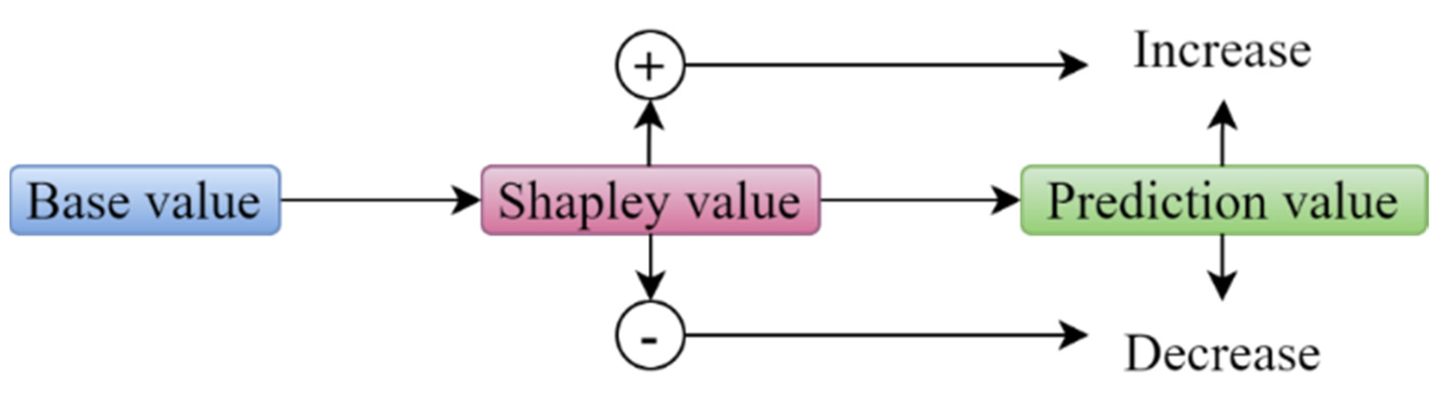
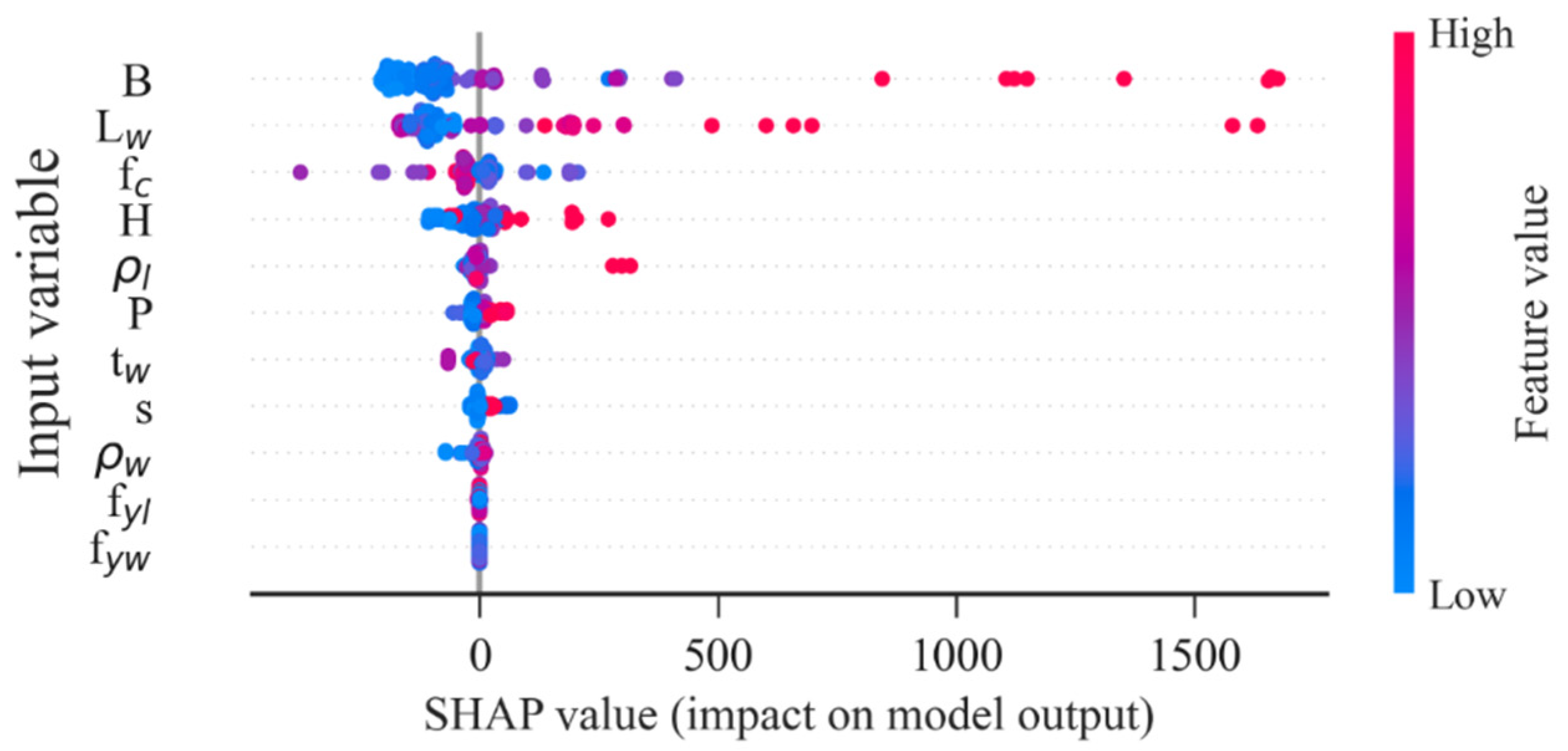
6.5. Explanation of the ML Models Using the SHAP Method

This section uses the SHAP method [69] to explore the feature importance and interpret the MFO-XGB model’s predictions. The SHAP method uses game theory to determine how parameters affect the response. The SHAP method assigns the input features an average importance value for a given prediction. It is advantageous to use the SHAP value because it reflects how the feature influences each sample positively and negatively. The influence of the Shapley value on the prediction value is depicted in Figure 14.

Figure 15 shows the feature relative importance plot, which ranks the features’ importance in identifying the failure modes. The features’ importance values are the mean absolute SHAP values of each variable in the data. Different colors represent the failure modes. The color in each input variable indicates its effect on the failure modes. This figure shows that ${\mathrm{L}}_{\mathrm{v}}$ and $\mathrm{s}$ are the most critical and least important features, respectively, for classifying the FMs of RHRC columns.

A class with a wider range indicates that features are more important. For example, ${\mathrm{L}}_{\mathrm{v}}$ has the most critical effect on the FF mode (class 1). Meanwhile, ${\mathrm{f}}_{\mathrm{y}\mathrm{w}}$ has the most significant impact on the SF mode (class 2) and FSF mode (class 3). Additionally, ${\mathrm{f}}_{\mathrm{y}\mathrm{l}}$ has a significant effect on the SF mode (class 2). The effect of input variables on each failure mode is depicted in Figure 16.

The relative importance of input variables are depicted in Figure 17 for each failure mode. The most important feature to each class is located at the top of the figure. In Figure 17, the red and blue dots indicate high and low feature values. The high SHAP value of the feature increases the likelihood of the failure mode with a slight increase in the corresponding value. Figure 17a shows that when ${\mathrm{L}}_{\mathrm{v}}$ increases, the SHAP value increases, and the model tends to show FF. Figure 17b depicts that the higher value of ${\mathrm{t}}_{\mathrm{w}}$ corresponds to a lower SHAP value, and the model tends to show SF. However, when $\mathrm{B}$ increases, the model tends to show FSF, as shown in Figure 17c. The variations of other parameters on the failure modes can be explained similarly.

The effects of the input parameters on predicting the shear strength of RHRC columns are presented in Figure 18. A SHAP summary plot of the regression MFO-XGB model is presented in Figure 19, where each dot is an individual data point in the dataset. These figures show that the most influential feature to shear strength is $\mathrm{B}$, followed by ${\mathrm{L}}_{\mathrm{v}}$, ${\mathrm{f}}_{\mathrm{c}}^{\prime }$, $\mathrm{H}$, ${\mathsf{\rho }}_{\mathrm{l}}$, $\mathrm{P}$, ${\mathrm{t}}_{\mathrm{w}}$, $\mathrm{s}$, ${\mathsf{\rho }}_{\mathrm{w}}$, ${\mathrm{f}}_{\mathrm{y}\mathrm{l}}$, and ${\mathrm{f}}_{\mathrm{y}\mathrm{w}}$. Moreover, Figure 19 shows that shear strength increases when $\mathrm{B}$, ${\mathrm{L}}_{\mathrm{v}}$, and $\mathrm{H}$ increase, while an increase in ${\mathrm{f}}_{\mathrm{c}}^{\prime }$ will lead to a decrease in shear strength.

This study also develops a web application (WA) based on the proposed classification and regression XGB models to help potential users and designers assess the failure modes and shear strength of RHRC columns. To use this WA, the eleven numeric values of ${\mathrm{L}}_{\mathrm{v}}$, $\mathrm{B}$, $\mathrm{H}$, ${\mathrm{t}}_{\mathrm{w}}$, ${\mathsf{\rho }}_{\mathrm{l}}$, ${\mathsf{\rho }}_{\mathrm{w}}$, $\mathrm{s}$, ${\mathrm{f}}_{\mathrm{c}}^{\prime }$, ${\mathrm{f}}_{\mathrm{y}\mathrm{l}}$, ${\mathrm{f}}_{\mathrm{y}\mathrm{w}}$, and $\mathrm{P}$ are required to predict the failure modes and the shear strength of RHRC columns. The WA allows users with limited coding experience to adopt and apply in structural engineering, safety and design applications. It helps to immediately obtain the results. The WA is provided freely in the link: https://sakat92-rhrc-rhrc-yqci89.streamlit.app (accessed on 6 June 2023).

7. Conclusions

The failure mode classification and shear strength prediction of RHRC columns are complex engineering tasks. This study investigates the performance of eight ML models, including SVM, MLP, KNN, DT, RF, AGB, GB, and XGB, for classifying the failure modes and predicting the shear strength of RHRC columns. The key findings of this study are as follows:

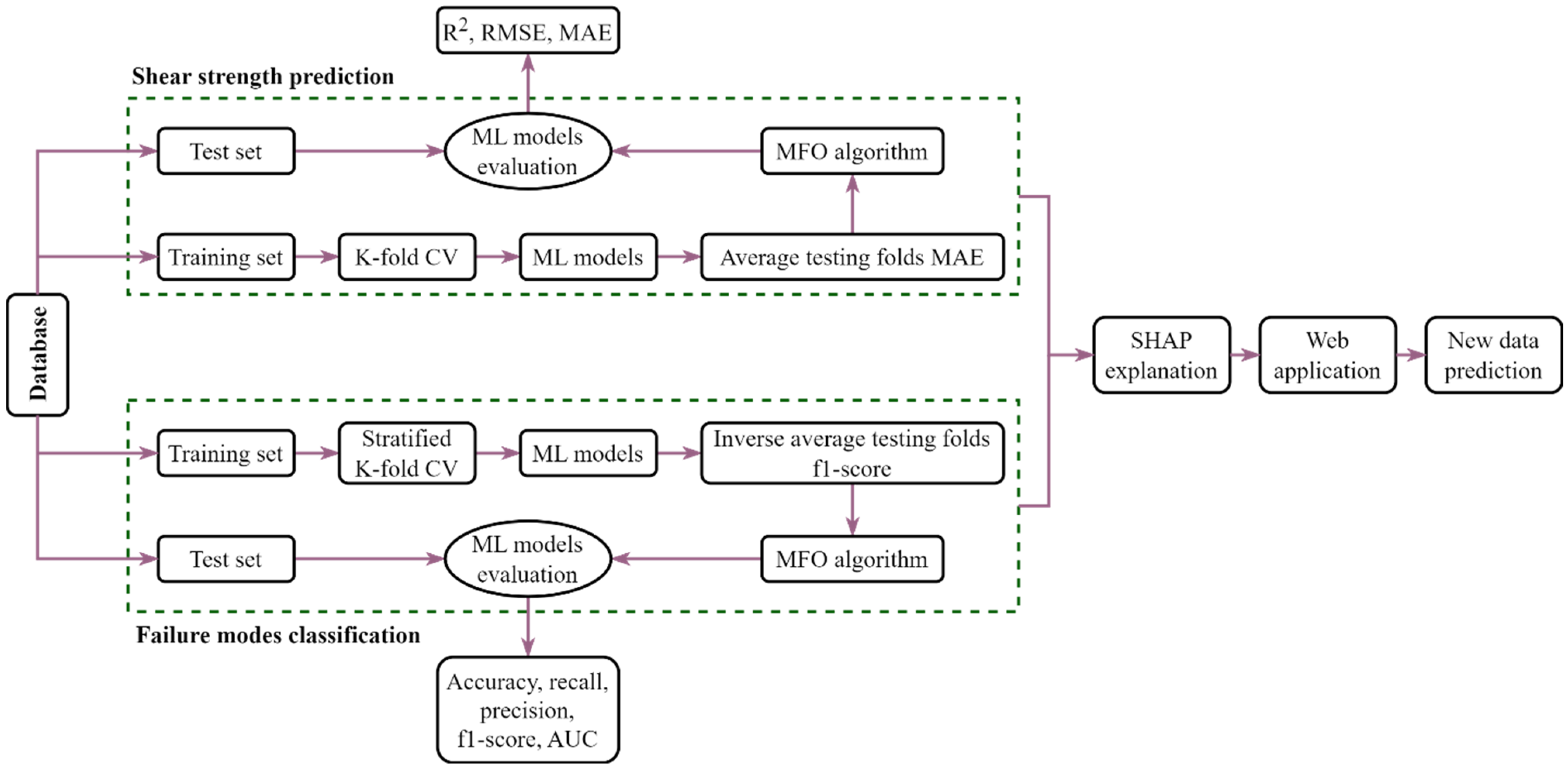
• Since failure modes are highly unbalanced, the SMOTE technique deals with the class imbalance of the database for the failure mode problems.
• MFO has proven to be highly appropriate for fine-tuning the hyperparameters of the ML models.
• Among the ML models, the MFO-XGB model outperforms others in both classifying the failure modes (accuracy of 92.9% for test set) and predicting the shear strength (${\mathrm{R}}^2$= 0.996 for test set) of RHRC columns. In addition, the results indicate that the MFO-XGB model is more accurate than the empirical models for shear strength prediction.
• According to the SHAP method, ${\mathrm{L}}_{\mathrm{v}}$ is the most influential feature to the FF mode and ${\mathrm{f}}_{\mathrm{y}\mathrm{w}}$ for the SF and FSF modes. $\mathrm{B}$ is the most influential feature to the shear strength prediction of RHRC columns.
• This study develops a web application, an engineer-friendly tool, that civil engineers can conveniently use in practice with less computational cost and effort. The web link of the WA can be found at https://sakat92-rhrc-rhrc-yqci89.streamlit.app (accessed on 6 June 2023).

It is noted that the developed ML models in this study only confidently apply to the database with the range of parameters indicated in Figure 4. Therefore, the ML models should be retrained when the database is updated. The current study dealt with predicting the shear strength and identifying the failure modes of hollow RC columns. However, other important issues such as prediction of plastic hinge length and ductility ratio of this column should be studied in future works.

References

1. Kim, T.-H.; Lee, J.-H.; Shin, H.M. Performance assessment of hollow RC bridge columns with triangular reinforcement details. Mag. Concr. Res. 2014, 66, 809–824. [Google Scholar] [CrossRef]
2. Cassese, P. Seismic Performance of Existing Hollow Reinforced Concrete Bridge Columns. Ph.D. Thesis, Department of Structures for Engineering and Architecture, University of Naples Federico II, Naples, Italy, 2017. [Google Scholar]
3. Cassese, P.; De Risi, M.T.; Verderame, G.M. Seismic assessment of existing hollow circular reinforced concrete bridge piers. J. Earthq. Eng. 2020, 24, 1566–1601. [Google Scholar] [CrossRef]
4. Cassese, P.; De Risi, M.T.; Verderame, G.M. A modelling approach for existing shear-critical RC bridge piers with hollow rectangular cross section under lateral loads. Bull. Earthq. Eng. 2019, 17, 237–270. [Google Scholar] [CrossRef]
5. Qi, Y.-L.; Han, X.-L.; Ji, J. Failure mode classification of reinforced concrete column using Fisher method. J. Cent. South Univ. 2013, 20, 2863–2869. [Google Scholar] [CrossRef]
6. Feng, D.-C.; Liu, Z.-T.; Wang, X.-D.; Jiang, Z.-M.; Liang, S.-X. Failure mode classification and bearing capacity prediction for reinforced concrete columns based on ensemble machine learning algorithm. Adv. Eng. Inf. 2020, 45, 101126. [Google Scholar] [CrossRef]
7. Zhu, L.; Elwood, K.; Haukaas, T. Classification and seismic safety evaluation of existing reinforced concrete columns. J. Struct. Eng. 2007, 133, 1316–1330. [Google Scholar] [CrossRef]
8. Ma, Y.; Gong, J.-X. Probability identification of seismic failure modes of reinforced concrete columns based on experimental observations. J. Earthq. Eng. 2018, 22, 1881–1899. [Google Scholar] [CrossRef]
9. Ghee, A.B.; Priestley, M.N.; Paulay, T. Seismic shear strength of circular reinforced concrete columns. Struct. J. 1989, 86, 45–59. [Google Scholar]
10. Ning, C.-L.; Feng, D.-C. Probabilistic indicator to classify the failure mode of reinforced-concrete columns. Mag. Concr. Res. 2019, 71, 734–748. [Google Scholar] [CrossRef]
11. Berry, M.; Parrish, M.; Eberhard, M. PEER Structural Performance Database User’s Manual (Version 1.0); University of California: Berkeley, CA, USA, 2004. [Google Scholar]
12. Yang, C.; Xie, L.; Li, A. Full-scale Experimental and Numerical Investigations on Seismic Performance of Square RC Frame Columns with Hollow Sections. J. Earthq. Eng. 2022, 26, 427–448. [Google Scholar] [CrossRef]
13. Yeh, Y.-K.; Mo, Y.; Yang, C. Full-scale tests on rectangular hollow bridge piers. Mater. Struct. 2002, 35, 117–125. [Google Scholar] [CrossRef]
14. Hwang, S.-J.; Lee, H.-J. Strength prediction for discontinuity regions by softened strut-and-tie model. J. Struct. Eng. 2002, 128, 1519–1526. [Google Scholar] [CrossRef]
15. Sezen, H. Shear deformation model for reinforced concrete columns. Struct. Eng. Mech. 2008, 28, 39–52. [Google Scholar] [CrossRef]
16. Vecchio, F.J.; Collins, M.P. The modified compression-field theory for reinforced concrete elements subjected to shear. ACI Struct. J. 1986, 83, 219–231. [Google Scholar]
17. Bentz, E.C.; Vecchio, F.J.; Collins, M.P. Simplified modified compression field theory for calculating shear strength of reinforced concrete elements. ACI Struct. J. 2006, 103, 614–624. [Google Scholar]
18. Hsu, T.T. Softened truss model theory for shear and torsion. Struct. J. 1988, 85, 624–635. [Google Scholar]
19. Pang, X.-B.D.; Hsu, T.T. Fixed angle softened truss model for reinforced concrete. Struct. J. 1996, 93, 196–208. [Google Scholar]
20. Muttoni, A.; Fernández Ruiz, M. Shear strength of members without transverse reinforcement as function of critical shear crack width. A ACI Struct. J. 2008, 105, 163–172. [Google Scholar]
21. Feng, D.-C.; Wu, G.; Sun, Z.-Y.; Xu, J.-G. A flexure-shear Timoshenko fiber beam element based on softened damage-plasticity model. Eng. Struct. 2017, 140, 483–497. [Google Scholar] [CrossRef]
22. Ascheim, M.; Moehle, J. Shear Strength and Deformability of RC Bridge Columns Subjected to Inelastic Cyclic Displacements; Technical Report No. UCB/EERC-92/04; University of California: Berkeley, CA, USA, 1992. [Google Scholar]
23. Priestley, M.N.; Verma, R.; Xiao, Y. Seismic shear strength of reinforced concrete columns. J. Struct. Eng. 1994, 120, 2310–2329. [Google Scholar] [CrossRef]
24. Kowalsky, M.J.; Priestley, M.N. Improved analytical model for shear strength of circular reinforced concrete columns in seismic regions. ACI Struct. J. 2000, 97, 388–396. [Google Scholar]
25. Sezen, H.; Moehle, J.P. Shear strength model for lightly reinforced concrete columns. J. Struct. Eng. 2004, 130, 1692–1703. [Google Scholar] [CrossRef]
26. Biskinis, D.E.; Roupakias, G.K.; Fardis, M.N. Degradation of shear strength of reinforced concrete members with inelastic cyclic displacements. ACI Struct. J. 2004, 101, 773–783. [Google Scholar]
27. ACI-318; ACI 318-14: Building Code Requirements for Structural Concrete and Commentary. American Concrete Institution: Indianapolis, IN, USA, 2014.
28. EN-1998-1; Eurocode 8: Design of Structures for Earthquake Resistance-Part 1: General Rules. Seismic Actions and Rules for Buildings. European Committee for Standardization: Brussels, Belgium, 2004.
29. Shin, M.; Choi, Y.Y.; Sun, C.-H.; Kim, I.-H. Shear strength model for reinforced concrete rectangular hollow columns. Eng. Struct. 2013, 56, 958–969. [Google Scholar] [CrossRef]
30. Zhang, Y.-Y.; Harries, K.A.; Yuan, W.-C. Experimental and numerical investigation of the seismic performance of hollow rectangular bridge piers constructed with and without steel fiber reinforced concrete. Eng. Struct. 2013, 48, 255–265. [Google Scholar] [CrossRef]
31. Xie, Y.; Ebad Sichani, M.; Padgett, J.E.; DesRoches, R. The promise of implementing machine learning in earthquake engineering: A state-of-the-art review. Earthq. Spectra 2020, 36, 1769–1801. [Google Scholar] [CrossRef]
32. Gharehbaghi, S.; Yazdani, H.; Khatibinia, M. Estimating inelastic seismic response of reinforced concrete frame structures using a wavelet support vector machine and an artificial neural network. Neural Comput. Appl. 2020, 32, 2975–2988. [Google Scholar] [CrossRef]
33. Khademi, F.; Akbari, M.; Nikoo, M. Displacement determination of concrete reinforcement building using data-driven models. Int. J. Sustain. Built Environ. 2017, 6, 400–411. [Google Scholar] [CrossRef]
34. Zhang, Y.; Burton, H.V.; Sun, H.; Shokrabadi, M. A machine learning framework for assessing post-earthquake structural safety. Struct. Saf. 2018, 72, 1–16. [Google Scholar] [CrossRef]
35. Huang, H.; Burton, H.V. Classification of in-plane failure modes for reinforced concrete frames with infills using machine learning. J. Build. Eng. 2019, 25, 100767. [Google Scholar] [CrossRef]
36. Mangalathu, S.; Sun, H.; Nweke, C.C.; Yi, Z.; Burton, H.V. Classifying earthquake damage to buildings using machine learning. Earthq. Spectra 2020, 36, 183–208. [Google Scholar] [CrossRef]
37. Mangalathu, S.; Hwang, S.-H.; Choi, E.; Jeon, J.-S. Rapid seismic damage evaluation of bridge portfolios using machine learning techniques. Eng. Struct. 2019, 201, 109785. [Google Scholar] [CrossRef]
38. Naderpour, H.; Mirrashid, M. Shear failure capacity prediction of concrete beam–column joints in terms of ANFIS and GMDH. Pract. Period. Struct. Des. Constr. 2019, 24, 04019006. [Google Scholar] [CrossRef]
39. Mangalathu, S.; Hwang, S.-H.; Jeon, J.-S. Failure mode and effects analysis of RC members based on machine-learning-based SHapley Additive exPlanations (SHAP) approach. Eng. Struct. 2020, 219, 110927. [Google Scholar] [CrossRef]
40. Thai, D.-K.; Tu, T.M.; Bui, T.Q.; Bui, T.-T. Gradient tree boosting machine learning on predicting the failure modes of the RC panels under impact loads. Eng. Comput. 2021, 37, 597–608. [Google Scholar] [CrossRef]
41. Mangalathu, S.; Jeon, J.-S. Machine learning–based failure mode recognition of circular reinforced concrete bridge columns: Comparative study. J. Struct. Eng. 2019, 145, 04019104. [Google Scholar] [CrossRef]
42. Phan, V.-T.; Tran, V.-L.; Nguyen, V.-Q.; Nguyen, D.-D. Machine learning models for predicting shear strength and identifying failure modes of rectangular RC columns. Buildings 2022, 12, 1493. [Google Scholar] [CrossRef]
43. Mander, J.; Priestley, M.; Park, R. Behaviour of ductile hollow reinforced concrete columns. Bull. N. Z. Soc. Earthq. Eng. 1983, 16, 273–290. [Google Scholar] [CrossRef]
44. Sun, Z.; Wang, D.; Wang, T.; Wu, S.; Guo, X. Investigation on seismic behavior of bridge piers with thin-walled rectangular hollow section using quasi-static cyclic tests. Eng. Struct. 2019, 200, 109708. [Google Scholar] [CrossRef]
45. Calvi, G.M.; Pavese, A.; Rasulo, A.; Bolognini, D. Experimental and numerical studies on the seismic response of RC hollow bridge piers. Bull. Earthq. Eng. 2005, 3, 267–297. [Google Scholar] [CrossRef]
46. Mo, Y.; Nien, I. Seismic performance of hollow high-strength concrete bridge columns. J. Bridge Eng. 2002, 7, 338–349. [Google Scholar] [CrossRef]
47. Han, Q.; Zhou, Y.; Du, X.; Huang, C.; Lee, G.C. Experimental and numerical studies on seismic performance of hollow RC bridge columns. Earthq. Struct. 2014, 7, 251–269. [Google Scholar] [CrossRef]
48. Cheng, C.-T.; Yang, J.-C.; Yeh, Y.-K.; Chen, S.-E. Seismic performance of repaired hollow-bridge piers. Constr. Build. Mater. 2003, 17, 339–351. [Google Scholar] [CrossRef]
49. Faria, R.; Pouca, N.V.; Delgado, R. Simulation of the cyclic behaviour of R/C rectangular hollow section bridge piers via a detailed numerical model. J. Earthq. Eng. 2004, 8, 725–748. [Google Scholar] [CrossRef]
50. Mangalathu, S.; Jeon, J.-S. Classification of failure mode and prediction of shear strength for reinforced concrete beam-column joints using machine learning techniques. Eng. Struct. 2018, 160, 85–94. [Google Scholar] [CrossRef]
51. Gao, X.; Lin, C. Prediction model of the failure mode of beam-column joints using machine learning methods. Eng. Failure Anal. 2021, 120, 105072. [Google Scholar] [CrossRef]
52. Pedregosa, F.; Varoquaux, G.; Gramfort, A.; Michel, V.; Thirion, B.; Grisel, O.; Blondel, M.; Prettenhofer, P.; Weiss, R.; Dubourg, V.; et al. Scikit-learn: Machine learning in Python. J. Mach. Learn Res. 2011, 12, 2825–2830. [Google Scholar]
53. Smola, A.J.; Schölkopf, B. A tutorial on support vector regression. Stat. Comput. 2004, 14, 199–222. [Google Scholar] [CrossRef]
54. Deka, P.C. Support vector machine applications in the field of hydrology: A review. Appl. Soft Comput. 2014, 19, 372–386. [Google Scholar]
55. Rumelhart, D.E.; Hinton, G.E.; Williams, R.J. Learning representations by back-propagating errors. Nature 1986, 323, 533–536. [Google Scholar] [CrossRef]
56. Cover, T.; Hart, P. Nearest neighbor pattern classification. IEEE Trans. Inf. Theory 1967, 13, 21–27. [Google Scholar] [CrossRef]
57. Breiman, L.; Friedman, J.; Stone, C.J.; Olshen, R.A. Classification and Regression Trees; CRC Press: Boca Raton, FL, USA, 1984. [Google Scholar]
58. Breiman, L. Random forests. Mach. Learn. 2001, 45, 5–32. [Google Scholar] [CrossRef]
59. Ferreira, A.J.; Figueiredo, M.A. Boosting algorithms: A review of methods, theory, and applications. In Ensemble Machine Learning: Methods and Applications; Springer: New York, NY, USA, 2012; pp. 35–85. [Google Scholar]
60. Mirjalili, S. Moth-flame optimization algorithm: A novel nature-inspired heuristic paradigm. Knowl. Based Syst. 2015, 89, 228–249. [Google Scholar] [CrossRef]
61. Chawla, N.V.; Bowyer, K.W.; Hall, L.O.; Kegelmeyer, W.P. SMOTE: Synthetic minority over-sampling technique. J. Artif. Intell. Res. 2002, 16, 321–357. [Google Scholar] [CrossRef]
62. Hutter, F.; Kotthoff, L.; Vanschoren, J. Automated Machine Learning: Methods, Systems, Challenges; Springer Nature: Berlin/Heidelberg, Germany, 2019. [Google Scholar]
63. Yang, L.; Shami, A. On hyperparameter optimization of machine learning algorithms: Theory and practice. Neurocomputing 2020, 415, 295–316. [Google Scholar] [CrossRef]
64. Nguyen, V.-Q.; Tran, V.-L.; Nguyen, D.-D.; Sadiq, S.; Park, D. Novel hybrid MFO-XGBoost model for predicting the racking ratio of the rectangular tunnels subjected to seismic loading. Transp. Geotech. 2022, 37, 100878. [Google Scholar] [CrossRef]
65. Duan, J.; Asteris, P.G.; Nguyen, H.; Bui, X.-N.; Moayedi, H. A novel artificial intelligence technique to predict compressive strength of recycled aggregate concrete using ICA-XGBoost model. Eng. Comput. 2021, 37, 3329–3346. [Google Scholar] [CrossRef]
66. Tran, V.-L.; Kim, J.-K. Ensemble machine learning-based models for estimating the transfer length of strands in PSC beams. Expert Syst. Appl. 2023, 221, 119768. [Google Scholar] [CrossRef]
67. Nayak, J.; Naik, B.; Dash, P.B.; Souri, A.; Shanmuganathan, V. Hyper-parameter tuned light gradient boosting machine using memetic firefly algorithm for hand gesture recognition. Appl. Soft Comput. 2021, 107, 107478. [Google Scholar] [CrossRef]
68. Tran, V.-L.; Nguyen, D.-D. Novel hybrid WOA-GBM model for patch loading resistance prediction of longitudinally stiffened steel plate girders. Thin-Walled Struct. 2022, 177, 109424. [Google Scholar] [CrossRef]
69. Roth, A.E. Introduction to the Shapley value. In The Shapley Value; Cambridge University Press: Cambridge, UK, 1988; pp. 1–27. [Google Scholar]
Figure 1. Illustration of failure modes of RHRC columns.
Buildings 13 02914 g001
Figure 2. Dimensions and details of RHRC columns.
Buildings 13 02914 g002
Figure 3. Histograms of input parameters: (a) L v , (b) B, (c) H, (d) t w , (e) ρ l , (f) ρ w , (g) s, (h) f c , (i) f y l , (j) f y w , and (k) P.
Buildings 13 02914 g003
Figure 4. Histograms of output parameters: (a) shear strength, (b) failure modes.
Buildings 13 02914 g004
Figure 5. Flowchart of the MFO.
Buildings 13 02914 g005
Figure 6. Confusion matrix.
Buildings 13 02914 g006
Figure 7. K-fold cross-validation.
Buildings 13 02914 g007
Figure 8. Flowchart for developing ML models.
Buildings 13 02914 g008
Figure 9. Performance of classification ML models.
Buildings 13 02914 g009aBuildings 13 02914 g009b
Figure 10. ROC curves of the classification ML models.
Buildings 13 02914 g010aBuildings 13 02914 g010b
Figure 11. Shear strength prediction results of regression ML models.
Buildings 13 02914 g011
Figure 12. Statistic results of regression metrics for the test set after ten runs: (a) R2, (b) A10, (c) RMSE, and (d) MAE.
Buildings 13 02914 g012
Figure 13. Shear strength predictions of the MFO-XGB and empirical models for all data [4,22,23,24,25,26,29].
Buildings 13 02914 g013
Figure 14. Effect of Shapley value.
Buildings 13 02914 g014
Figure 15. Feature relative importance plot.
Buildings 13 02914 g015
Figure 16. SHAP value for each failure mode.
Buildings 13 02914 g016
Figure 17. Summary plot for each class.
Buildings 13 02914 g017
Figure 18. Relative importance of each feature.
Buildings 13 02914 g018
Figure 19. SHAP summary plot.
Buildings 13 02914 g019