Priority Needs for Facilities of Office Buildings in Thailand: A Copula-Based Ordinal Regression Model with Machine Learning Approach

Abstract

In the rapidly evolving business landscape of Thailand, the design and facilities of office buildings play a crucial role in enhancing employee satisfaction and productivity. This study seeks to answer the question: “How can office building facilities be optimized to meet the diverse preferences of occupants in Thailand, thereby improving their satisfaction and productivity”? This study employs a copula-based ordinal regression model combined with machine learning techniques to investigate the determinants of facility preferences in office buildings in Thailand. By analyzing data from 372 office workers in Bangkok, we identify the factors influencing facility needs and preferences, and measure the correlation between these preferences. Our findings reveal that safety and security are the highest-rated amenities, indicating their importance in the workplace. The findings reveal distinct preferences across demographic groups: age negatively influences the demand for certain amenities like lounges, while higher education levels increase the preference for cafeteria services. Employees in smaller firms show a higher preference for lounges and fitness centers but lower for restaurants and cafeterias. Interestingly, the size of the enterprise does not significantly affect preferences for fundamental facilities like security and cleaning. The study also uncovers the significant role of gender and income in shaping preferences for certain facilities. These results suggest that while basic amenities are universally valued, luxury or leisure-oriented facilities are more appreciated in smaller, possibly more community-focused work environments. This study highlights the need for tailored facility management in office buildings, considering the diverse needs of different employee groups, which has significant implications for enhancing workplace satisfaction and productivity.

1. Introduction

The provision of facilities in office buildings is crucial for sustainability, corporate social responsibility, economic rent, and overall building performance [1]. The significance of facilities within office buildings cannot be overstated, as they are essential in fostering not only the well-being and productivity of the workforce but also in attracting and retaining talent in a highly competitive business environment [2]. The correlation between well-designed office facilities and employee satisfaction and productivity is clear [3]. Some scholars underscored the importance of aligning office design with the needs of its users, suggesting that employees who are satisfied with their physical environment are more likely to produce better work outcomes [4,5]. Ornetzeder et al. demonstrated that the availability and maintenance of office equipment and facilities directly influences user satisfaction and well-being [6]. Aswin and Santhosh emphasized that the absolute best results cannot be achieved without the best office equipment and a good harmonious office environment [7]. Wang et al. proposed an integrated maintenance–safety framework that not only improves the safety and maintenance efficiency of facilities, but also enhances user satisfaction and well-being [8]. Fu et al. argued that innovative design strategies and technological applications in the post-pandemic era can create office environments that protect against the spread of pandemics as well as enhance employee well-being [9]. Therefore, a comprehensive understanding of the priority needs for facilities in office buildings is of paramount importance.

Thailand’s robust economic growth, driven by industries such as manufacturing, tourism, and services, has attracted local and international businesses. This has led to a surge in demand for office spaces in major cities like Bangkok, Chiang Mai, and Pattaya. Urbanization and the concentration of economic activities have further fueled the development of office buildings. There are a few studies focused on needs for office building in Thailand. For example, Einola et al. explored the integration of smart workplace solutions (SWS) in facilities management (FM) to make offices more user-centered [10]. Kofoworola and Gheewala highlighted that almost all commercial office buildings in Thailand follow similar structural and usage patterns, providing crucial information for understanding the baseline requirements for office facilities in the country [11]. Ongwandee et al. emphasized the importance of investigating volatile organic compounds (VOCs) in office buildings in Bangkok, Thailand, indicating the significance of indoor air quality in such environments [12]. Furthermore, Saengsawang and Panichpathom provided insights into the environmental perception and job satisfaction in certified office buildings in Thailand, underlining the importance of creating a conducive and satisfactory work environment for occupants [13]. Moreover, Pratiwi et al. emphasized the implementation of occupational health and safety standards in office buildings, highlighting the importance of facilities such as toilets and hand washing facilities for maintaining a healthy work environment [14]. Similarly, Surawattanasakul et al. focused on the prevalence of Sick Building Syndrome (SBS) among office workers in a healthcare setting and its association with indoor air quality (IAQ) [15]. This underscores the significance of providing adequate health and safety facilities for office occupants. Therefore, we can find that the needs for facilities in office buildings in Thailand encompass various aspects including structural design, indoor air quality, occupant satisfaction, health and safety standards, etc.

Previous scholars have also utilized various methods or models in studying issues related to office facilities. For example, Turpin-Brooks and Viccars emphasize the importance of effective post-occupancy evaluation (POE) as part of a sustainable approach to workplaces [16]. They highlight the need for robust methods of POE to guide facilities’ professionals in their choice of evaluation tools. Similarly, Li et al. conducted a comprehensive review of POE, providing both qualitative and quantitative insights, including a statistical analysis of POE projects and a comparison of existing POE protocols [17]. Artan et al. adopted a methodology involving literature review, expert interviews, and a field survey to acquire empirical data on the influence of office building design on occupant satisfaction [18]. Furthermore, Leung et al. utilized statistical techniques, including reliability tests, correlation coefficients, and multiple regression models, to analyze the interactions between facilities management and the environment domain of quality of life for older people in private buildings [19]. Likewise, Wang et al. analyzed the Pearson’s correlation coefficient between the level of maintenance and the level of safety in educational facilities, and the study found that there was a correlation of 0.74 between the two [8]. Göçer et al. conducted regression analyses and two-way ANOVA tests using POE survey data to understand the differences in occupants’ satisfaction and perceived productivity arising from open-plan offices [20]. Additionally, Kim and Kim examined the relationship between the “green” identity of an office building and occupants’ attitude toward the building, as well as the effect of occupants’ expectations and perceptions on their overall satisfaction [21]. The literature also highlights the use of questionnaires and Likert-type scales to measure attitudes and satisfaction, as demonstrated by [22,23]. These studies utilized post-occupancy questionnaires and statistical analyses to evaluate occupant satisfaction and building performance. To sum up, these methodologies provide valuable insights into occupant satisfaction, building performance, and the impact of design and environmental factors on occupants’ needs and preferences.

The existing body of research on office building facilities has made significant contributions to understanding occupant needs and satisfaction. However, despite the progress made in this field, several research gaps and limitations persist. Firstly, there is a lack of comprehensive analysis of functional requirements for office building facilities. While previous studies have examined specific aspects such as indoor environmental quality, space layout, and building aesthetics, a holistic approach that integrates various functional needs is warranted. Secondly, the diverse and varied nature of users’ demands for office building facilities necessitates a more in-depth analysis of the determinants of each specific requirement. Understanding the factors that drive different occupant needs is crucial for tailoring building facilities to meet diverse user preferences effectively. Thirdly, the predominant use of qualitative research methods and models in existing studies highlights the need for greater application of advanced quantitative methodologies. While qualitative approaches provide valuable insights, the incorporation of advanced quantitative techniques can enhance the rigor and depth of the analyses, leading to more robust and generalizable findings.

The aim of this study is to investigate the determinants of facility preferences in office buildings and measure the correlation between these preferences using the copula ordinal regression model and machine learning techniques. By utilizing the copula ordinal regression model, this research aims to identify the factors influencing facility needs and preferences in office buildings. Furthermore, the study employs elastic net regularization regression to overcome issues related to multicollinearity and overfitting. Compared with traditional ordinal models [24,25], the copula-based bivariate ordinal regression model, as highlighted by Hernández-Alava and Pudney [26] and Suknark et al. [27], offers a robust framework for understanding dependent ordinal data. Its ability to capture the dependency structure between multiple ordinal outcomes makes it superior for analyzing correlated preferences. Meanwhile, the elastic net regularization regression, as developed by Wurm et al. [28], effectively deals with multicollinearity and overfitting by combining L₁ and L₂ penalties. This method has been shown to provide better prediction accuracy and interpretability in variable selection than traditional regression models [29].

The main contributions of this study are threefold. First, this paper classifies the facility usage needs of office buildings into twelve distinct categories: security, safety, cleaning, banking, postal, convenience stores, restaurant, cafeteria, commuting, lounges, fitness center, and food trucks. Such detailed categorization allows for a comprehensive analysis of office building facility needs. Second, by considering the correlations among facility demands, this study is the first to employ a copula ordinal regression model for analyzing the determinants of office facility needs. This innovative approach provides a better understanding of the complex interplay between different facility preferences. Last but not least, diverging from previous studies, this paper adopts an elastic net regularization regression and Post-Double Selection (PDS) approach to filter determinants, overcoming the issues of multicollinearity and overfitting that are common in such research. This methodology ensures a more reliable and robust model for predicting facility needs in office buildings. Therefore, the findings of this study are poised to inform stakeholders in the real estate and facilities management sectors about the prioritization of office building facilities. By integrating a copula ordinal regression model with elastic net regularization, this research not only advances the methodological toolkit available for empirical analysis but also offers practical implications for designing and managing office spaces that align with the nuanced needs of modern occupants.

The remainder of the article is organized as follows. Section 2 describes the data. We review the elastic net regularization regression and bivariate copula-based ordinal regression model in Section 3. We employ the models to analyze the determinants of office facility needs in Section 4. Finally, Section 5 gives a conclusion and discusses limitations.

2. The Data

2.1. Questionnaire and Sampling Design

The survey questionnaire, designed as part of a research project titled “Demographic Characteristics and Amenities/Facilities Design for Worker Productivity: A Case Study of Multi-tenants Office Building in Bangkok CBD” under Thammasat Business School, comprises a comprehensive set of questions aimed at understanding the needs and preferences regarding office building amenities and facilities. Some key aspects of the survey are listed as follows:

(1) Number of questions: the survey contains a total of 69 questions, covering a wide range of topics related to office amenities and facilities. (2) Collection method: The survey is conducted online, accessible through a provided Google Forms link. This method allows for a broad and diverse range of participants. (3) Rewards for respondents: To appreciate the time and effort of the respondents, the survey offers a chance to win 1 of 26 Starbucks voucher cards through a lucky draw. The maximum prize value is 800 baht.

Some important questions included in the survey are designed as follows: (1) Demographic information: Questions regarding the respondent’s age, income level, and living situation. For example, age options range from “Under 18” to “36–41”, and income levels range from “Less than 20,000” to “80,001–100,000”. (2) Office location: respondents are asked about the location of their office building to understand geographical preferences. (3) Employment details: questions cover job status (e.g., “Full-time staff”, “Part-time staff”, “Intern”, “Freelancer”) and the sector of employment (e.g., “Commerce”, “Health Care Services”, “Media & Publishing”). (4) Amenities/facilities importance: a series of questions ask respondents to rate the importance of various amenities and facilities on a scale from “(5) Very important” to “(1)”.

In this study, the sampling process was carefully designed to ensure representativeness and reliability. First, we randomly selected 68 office buildings in the three main areas of Bangkok, namely Silom-Sathorn, Sukhumvit, and Central Lumpini, for the study in 2020. Then, we randomly selected 155 companies from these office buildings, covering businesses of different sizes, including small, medium, and large firms. Finally, we randomly sampled the office workers of these companies, and a total of 372 office workers participated in the survey. By randomly sampling both companies and employees, we ensured that the sample was representative and comparable, thus making the findings more generalizable and reliable. We classify the facility usage needs of office buildings into twelve distinct categories, which follows a systematic approach based on the analysis of data from 372 office workers in Bangkok. The categorization process involved identifying key amenities and services that are commonly found in office buildings and are essential for employee well-being and productivity. These categories were determined through a combination of literature review, expert consultations, and empirical data analysis. These categories are as follows: security, safety, cleaning, banking, postal services, convenience stores, restaurants, cafeterias, commuting facilities, lounges, fitness centers, and food trucks. Each category was defined to encapsulate a specific type of facility need that contributes to the overall functionality and satisfaction of office building occupants. This classification approach allowed us to systematically analyze the data and identify key determinants of facility preferences among office workers. The twelve categories represent a comprehensive framework for understanding the diverse and multifaceted needs of office building users in Bangkok.

This study adopts a comprehensive approach to analyze the determinants of office facility preferences, incorporating both demographic variables and control variables. The selection of these variables is based on three reasons. First, demographic variables (such as age, gender, and education level) are used in the study to capture differences in office facility preferences among different groups. These variables are generally considered fundamental factors influencing employees’ demands for office facilities. For example, younger employees might have a higher preference for fitness centers, whereas employees with higher education levels might lean more towards needing café services. Second, control variables (such as income level, type of housing, family size, pet ownership, company size, employment sector, and tenure with the current organization) are used to account for external factors that might influence office facility preferences. By controlling for these variables, the study can more accurately identify and analyze the main factors affecting facility preferences, reducing bias caused by other unobserved variables. Third, we utilize a variable selection method based on elastic net regularization regression and the Post-Double Selection (PDS) approach. This method combines L₁ and L₂ penalties, effectively dealing with issues of multicollinearity and overfitting, thereby improving the accuracy of variable selection and the predictive power of the model. Through this method, the study is able to filter out the most relevant variables from a large pool of potential explanatory variables, providing a solid foundation for constructing a copula-based ordinal regression model.

2.2. Data Analysis

Table 1. Data descriptive.

Variable	Type	Description	Mean	Min	Max
Dependent variables
Safety	Ordinal	The safety of assets of the company	4.6909	5.0000	2.0000
Security	Ordinal	The safety of human resources	4.6586	5.0000	2.0000
Cleaning	Ordinal	Cleaning and maintenance	4.5134	5.0000	0.0000
Convenience	Ordinal	Convenience store	4.2581	5.0000	0.0000
Restaurants	Ordinal	Restaurants	3.9167	5.0000	0.0000
Cafeteria	Ordinal	Cafeteria/Canteen	3.8575	5.0000	0.0000
Banking	Ordinal	Banking and financial services	3.8226	5.0000	0.0000
Postal	Ordinal	Postal services	3.5403	5.0000	0.0000
Commuting	Ordinal	Commuting solutions	3.4624	5.0000	0.0000
Lounges	Ordinal	Break room/Lounges	3.3306	5.0000	0.0000
Center	Ordinal	Fitness center/Gym	3.2500	5.0000	0.0000
Trucks	Ordinal	Food trucks	3.2124	5.0000	0.0000
Demographic variables
Age	Continuous	Worker’s age	33.4745	59.0000	20.5000
Male	Binary	Gender	0.3038	1.0000	0.0000
Female	Binary	Gender	0.6559	1.0000	0.0000
Education	Continuous	Educated years	16.7742	22.0000	12.0000
Control variables
I1	Binary	Average income per month (THB) 20,000–40,000 THB/Month	0.9301	1.0000	0.0000
I2	Binary	Average income per month (THB) 40,001–60,000 THB/Month	0.5511	1.0000	0.0000
I3	Binary	Average income per month (THB) 60,001–80,000 THB/Month	0.3360	1.0000	0.0000
I4	Binary	Average income per month (THB) 80,001–100,000 THB/Month	0.2097	1.0000	0.0000
I5	Binary	Average income per month (THB) More than 100,000 THB/Month	0.1290	1.0000	0.0000
D11	Binary	Housing type, housing estate	0.3817	1.0000	0.0000
D12	Binary	Housing type, condominium	0.4140	1.0000	0.0000
D13	Binary	Housing type, apartment flat mansion	0.1882	1.0000	0.0000
D14	Binary	Housing type, shop house	0.0941	1.0000	0.0000
D15	Binary	Housing type, others	0.3118	1.0000	0.0000
Famno	Ordinal	family number	3.0591	5.0000	1.0000
Pet	Binary	1 if the worker raises pets, 0 otherwise	0.2231	1.0000	0.0000
D21	Binary	Company Size, Large Enterprise	0.0376	1.0000	0.0000
D22	Binary	Company Size, Small Enterprise	0.2419	1.0000	0.0000
D23	Binary	Company Size, Medium Enterprise	0.2204	1.0000	0.0000
D32	Binary	Sector of your current company/organization, finance	0.2016	1.0000	0.0000
D33	Binary	Sector of your current company/organization, property and construction	0.2527	1.0000	0.0000
D35	Binary	Sector of your current company/organization, industry	0.0860	1.0000	0.0000
D36	Binary	Sector of your current company/organization, consumer products	0.0645	1.0000	0.0000
D37	Binary	Sector of your current company/organization, source company	0.0054	1.0000	0.0000
D41	Binary	No. of year working at current organization, less than 1 year	0.2177	1.0000	0.0000
D42	Binary	No. of year working at current organization, 1–2 years	0.1935	1.0000	0.0000
D43	Binary	No. of year working at current organization, 2–3 years	0.1290	1.0000	0.0000
D44	Binary	No. of year working at current organization, 3–4 years	0.0941	1.0000	0.0000

describes the type, mean, minimum, and maximum values of all variables. We categorize them into dependent, demographic, and control variables. Dependent variables are ordinal, reflecting office workers’ perceptions of workplace amenities such as safety, security, and convenience, with safety of assets and human resources rated highest on average. Demographic variables include continuous data on age and education, and binary data on gender. Control variables indicate income brackets, housing types, family size, pet ownership, company size, sector of employment, and tenure at the current organization. Notably, a majority of respondents fall within the 20,000 to 40,000 THB monthly income bracket and live in housing estates or condominiums. Company size distribution skews towards small and medium enterprises, and the workforce is predominantly female.

Some key points can also be drawn from Table 1. First, the highest-rated amenities among office workers are related to safety and security, with mean scores above 4.65, indicating that these aspects are likely well managed within the surveyed office buildings. Conversely, amenities such as food trucks, fitness centers, and lounges have lower mean scores, suggesting that these services may require improvement to meet employee expectations. Second, the workforce in the surveyed areas appears to be predominantly female, with approximately 65.59% of the respondents identifying as female and only 30.38% as male. This could reflect gender distribution in certain industries or roles that are prevalent in the prime areas of Bangkok. Third, the average number of educated years is 16.77, suggesting that the office workers in these prime areas are relatively well educated, which may correlate with the types of jobs available in these business districts.

Figure 1 describes a heat map of Spearman’s rho coefficients for dependent variables. A heat map in this context is likely a graphical representation of data where individual values contained in a matrix are represented as colors. Spearman’s rho is a non-parametric measure of rank correlation, indicating the strength and direction of association between two ranked variables [30]. We can find that the high correlation of cafeteria and restaurant with other variables in Figure 1. This suggests that in the surveyed office spaces, employees’ perceptions of dining facilities are strongly associated with other amenities and services. This indicates that employees consider dining facilities as an important factor when evaluating the workplace and link them with other convenience amenities and services. We also can find that the relationship between safety and security equals to 0.723, indicating that workers perceive these two factors in tandem when considering their workplace well-being. Conversely, amenities with weaker correlations, such as security and fitness center, security and lounges, may suggest areas where worker perceptions are more varied or less influenced by perceptions of these amenities.

3. Methodology

3.1. Copula-Based Bivariate Ordinal Regression Model

The copula-based bivariate ordinal regression model (CORM) is a valuable tool used in various fields such as medicine, demography, and social sciences. This model allows for the analysis of relationships between two ordered categorical response variables and one or more explanatory variables. One of the key advantages of this model is its flexibility in handling ordinal responses with more than two categories, providing a comprehensive understanding of the underlying relationships [31].

The basic structure of the CORM involves describing the relationship between two ordered categorical response variables and explanatory variables. Following Hernández-Alava and Pudney [26], the CORM in our study can be expressed as follows:

$$P_{i1}^{\mathrm{*}}=X_i{\beta }_1+Z_{i1}{\delta }_1+U_i$$

(1)

$$P_{i2}^{\mathrm{*}}=X_i{\beta }_2+Z_{i2}{\delta }_2+V_i$$

(2)

$$\mathrm{F}\left(U_i,V_i\right)=\mathrm{C}(G_1\left(U_i\right),{ G}_2\left(V_i\right);\rho )$$

(3)

$$P_{ij}=r \mathrm{iff} {\mathsf{\Gamma }}_{rj}\le P_{ij}^{\mathrm{*}}<{\mathsf{\Gamma }}_{r+1j} r=1,\dots ,R_j \mathrm{and} j=1,2$$

(4)

where $P_{i1}^{*}$ and $P_{i2}^{*}$ are latent variables that can be any facilities in the 12 categories. $X_i$ is the vector of treatment variables including age, education, income, and gender in this study. $Z_{i1}$ and $Z_{i2}$ are control variables that may be the same or overlap. The joint distribution of the two equations is $\mathrm{F}\left(U_i,V_i\right)$ and it equals to a copula function $\mathrm{C}(G_1\left(U_i\right),G_2\left(V_i\right);\rho )$ with copula parameter $\rho$. $G_i\left(.\right)$ is marginal distribution and is specified as mixtures of two normal components. The mixture distribution can capture skewness and shape, etc. [26]. The relationship between the latent variables and their observable counterparts is crucial for understanding the ordinal nature of the data and for modeling the probability of observing certain outcomes given the explanatory variables and the underlying distribution of the residuals characterized by a copula function [32,33].

Sklar proposed copula function and demonstrated its definition and properties; whereafter, many copula families were proposed [34]. In this study, some copula functions are used in the context of bivariate ordinal regressions. These copulas, including Gaussian, Clayton, Gumbel, Joe, and Frank, are used to model the residual dependence in the data, characterized by a copula function and normal mixture marginals. The Gaussian copula allows for both positive and negative dependence and exhibits symmetric dependence in both tails of the distribution. It is defined by a correlation coefficient $\rho$, which ranges between −1 and 1. The Clayton copula is suitable when there is strong left-tail dependence but weaker right-tail dependence, meaning that it captures scenarios where two variables are strongly correlated at low values but not as much at high values. It does not allow for negative dependence and is asymmetric in the tails. The Gumbel copula, like the Clayton, does not permit negative dependence and has asymmetric tail dependence. However, it exhibits weak left-tail dependence and strong right-tail dependence, with the right-tail dependence being stronger than in the Clayton copula. The Joe copula is similar to the Gumbel copula in that it does not allow for negative dependence and has strong right-tail dependence. However, the right-tail dependence in the Joe copula is even stronger than in the Gumbel, making it closer to the opposite of the Clayton copula in terms of its tail behavior. Lastly, the Frank copula can represent both positive and negative dependence, like the Gaussian copula, but it differs in that it shows weaker dependence in the tails and stronger dependence in the middle of the distribution [35,36]. Each of these copulas add flexibility to the modeling of residual dependence in bivariate ordinal regression models, allowing for a more accurate representation of the underlying data structure.

The different copula parameters have different ranges. To ensure that the parameters of maximum likelihood estimation are unconstrained, we set some smoothing transformation functions as follows.

$$\rho =\left\{\begin{array}{cc}\tanh (\delta )\hfill & \mathrm{G}\mathrm{a}\mathrm{u}\mathrm{s}\mathrm{s}\mathrm{i}\mathrm{a}\mathrm{n}, \mathsf{\rho }\in (-1,1)\hfill \\ e^{\delta }\hfill & \mathrm{C}\mathrm{l}\mathrm{a}\mathrm{y}\mathrm{t}\mathrm{o}\mathrm{n}, \mathsf{\rho }\in (0,+\infty )\hfill \\ \delta \hfill & \mathrm{F}\mathrm{r}\mathrm{a}\mathrm{n}\mathrm{k}, \mathsf{\rho }\in (-\infty ,+\infty )/0\hfill \\ e^{\delta }+1\hfill & \mathrm{G}\mathrm{u}\mathrm{m}\mathrm{b}\mathrm{e}\mathrm{l} \mathrm{a}\mathrm{n}\mathrm{d} \mathrm{J}\mathrm{o}\mathrm{e},\mathsf{\rho }\in (1,+\infty )\hfill \end{array}\right.$$

(5)

3.2. Control Variable Selection Based Elastic Net Regression

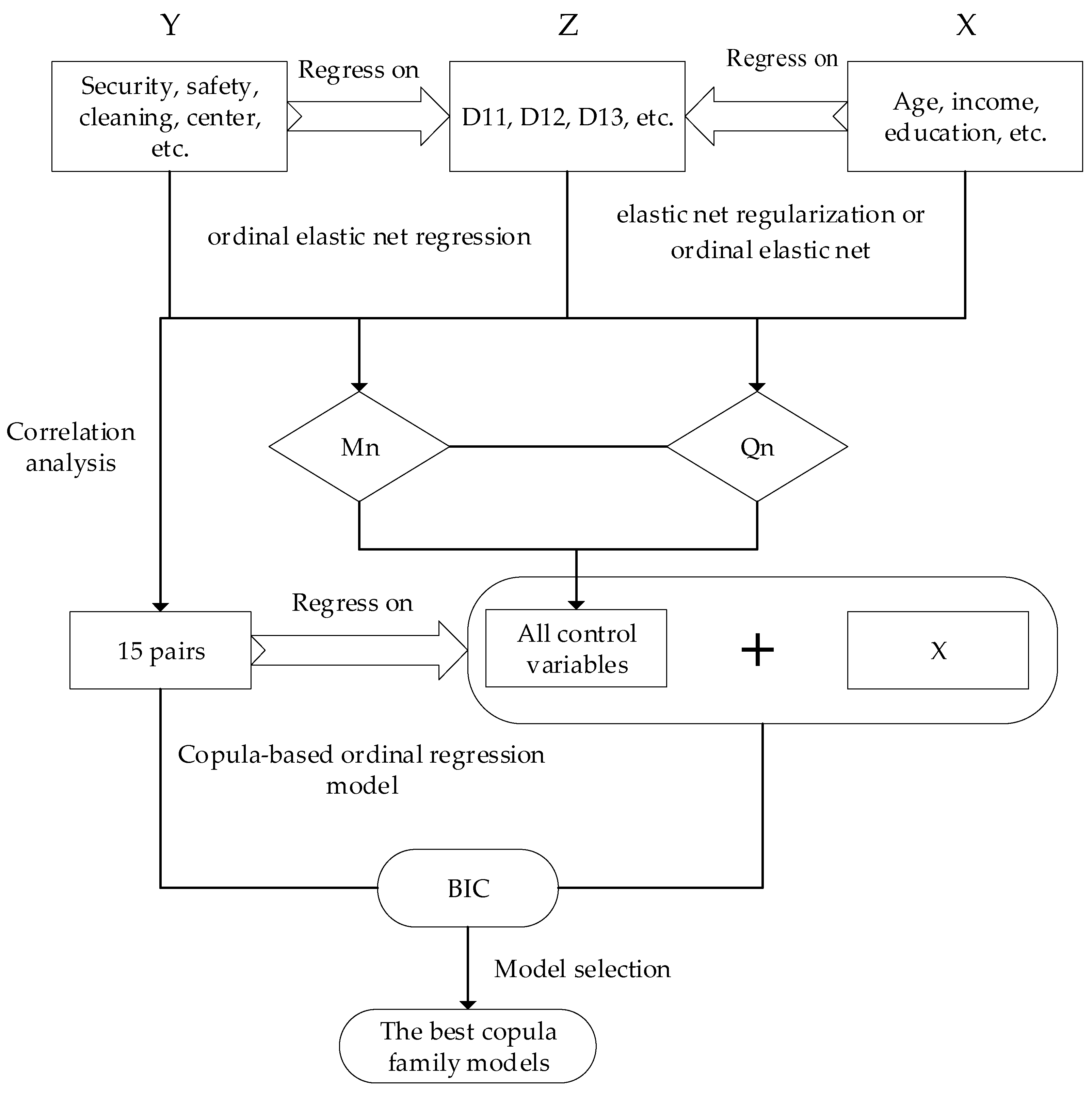
In regression models, we often are often concerned with the issue of biased missing variables, which leads to the problem of controlling variable selection. Referring to Post-Double Selection (PDS) approach [37] and ordinal elastic net regression [28], this study constructs the control variable selection approach based ordinal elastic net regression and PDS.

Ordinal elastic net regression is a machine learning method. Elastic net regression combines the penalties of both ridge regression and lasso regression, and by adjusting the mixing parameter, it can perform variable selection and handle multicollinearity in the predictor variables. The PDS is particularly useful when the researcher is interested in estimating the causal effect of a particular variable (the treatment variable) on an outcome variable, while controlling for a potentially large number of other covariates. The Post-Double Selection approach consists of two main steps: In the first step, two separate regressions are conducted. In the first regression, the outcome variable is regressed on all potential control variables, and the variables that are significantly associated with the outcome are selected. In the second regression, the treatment variable is regressed on all potential control variables, and again, the variables that are significantly associated with the treatment are selected. In the final step, the outcome variable is regressed on the treatment variable and the set of control variables selected in the first step. We draw inspiration from the PDS method and apply the ordinal elastic net regression to filter control variables. Finally, we use the copula-based bivariate ordinal regression model to analyze the preference and correlation issues of office building facility needs. The flowchart of our approach is in Figure 2, and the detailed steps of the approach are as follows:

Step 1:

Regress the ordered dependent variable y using the ordinal elastic net regression, where y is the ordered response variable and βj are the coefficients for all control variables. The log-likelihood function is expressed as follows:

$$-\mathrm{l}\mathrm{n} L(\beta ,\gamma )=-{\sum }_{\pi =1}^{\mathsf{\Pi }} {\sum }_{i=1}^n Z_{i\pi }\mathrm{l}\mathrm{n}[\varphi ({\gamma }_{\pi }-x_{i\beta })-({\gamma }_{\pi -1}-x_{i\beta })]+\lambda {\sum }_{j=1}^P (\alpha \left|{\beta }_j\right|+\frac{1}{2}(1-\alpha ){\beta }_j^2)$$

(6)

where $\lambda {\sum }_{j=1}^P (\alpha \left|{\beta }_j\right|+\frac{1}{2}(1-\alpha ){\beta }_j^2)$ is elastic net penalty and obtain Mn control variables.

Step 2:

for each treatment variable $X_f$, regress $X_f$ on Z using elastic net regularization or ordinal elastic net to obtain the set of selected control variables Qn, where f = 1, …, p.

Step 3:

all independent variables of each facility include Mn and Qn.

Step 4:

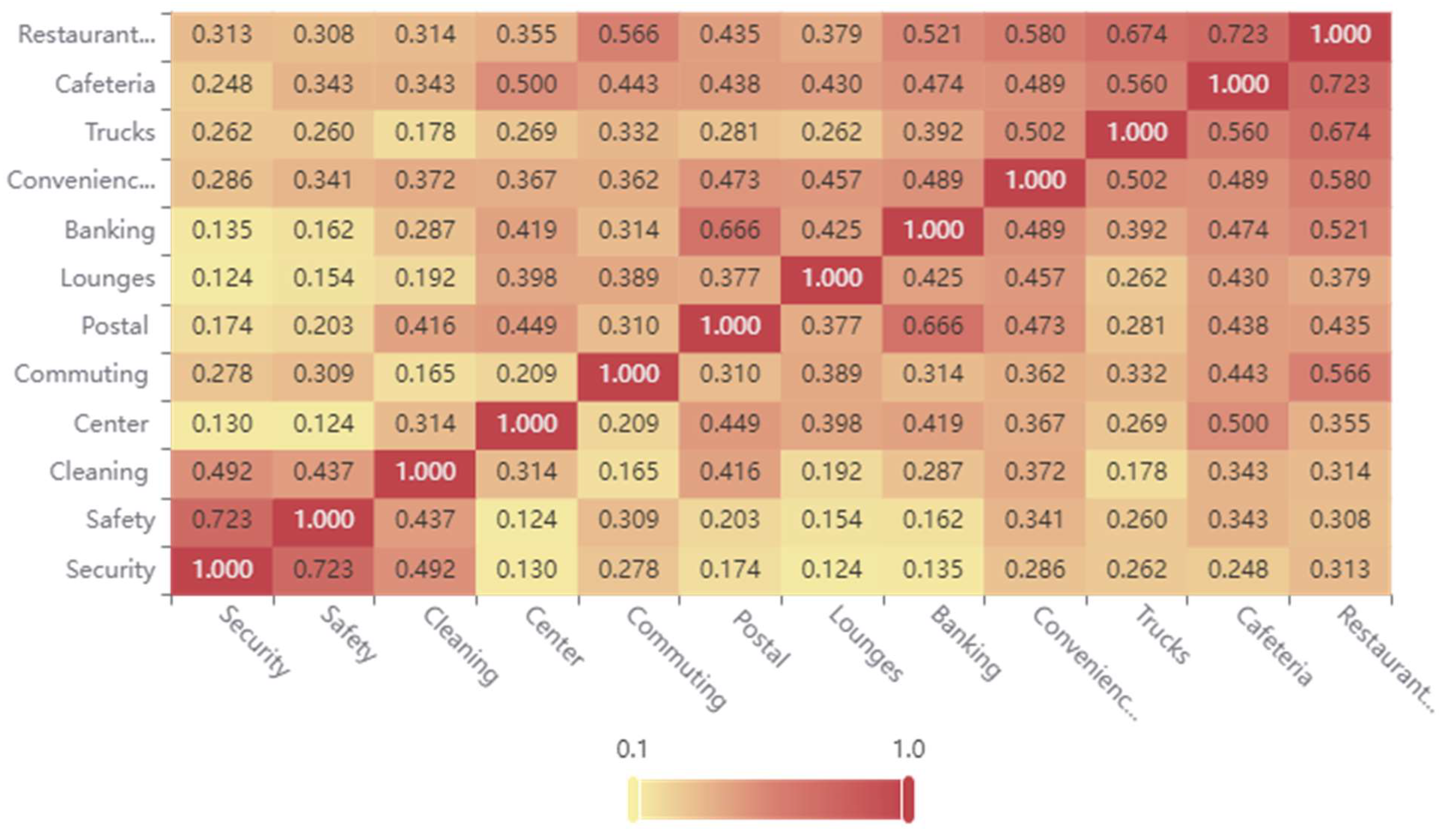
Construct the copula-based bivariate ordinal regression model with all independent variables and each pair of facilities. Note that we select 15 pairs of facilities in terms of correlation coefficient of all pairs.

Step 5:

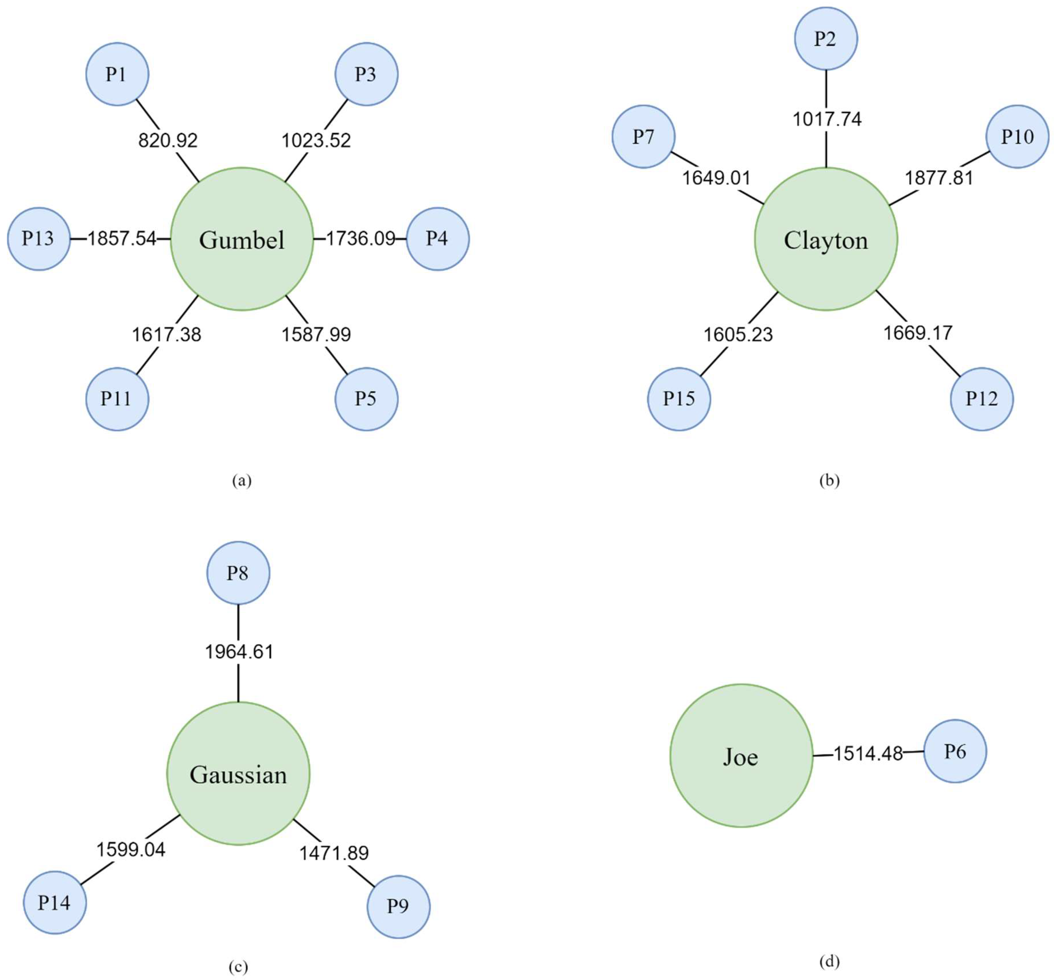
we calculate BIC values of all the copula-based bivariate ordinal regression model and select the best copula family based on BIC for each pair.

4. Empirical Results

Table 2. Estimated results of elastic net regression model.

	Age	Income	Female	Male	Education	Security	Safety	Cleaning	Postal
(Intercept): 1	No	Yes	Yes	Yes	No	Yes	Yes	Yes	Yes
(Intercept): 2	No	Yes	No	No	No	Yes	Yes	Yes	Yes
(Intercept): 3	No	Yes	No	No	No	Yes	Yes	Yes	Yes
(Intercept): 4	No	Yes	No	No	No	No	No	Yes	Yes
(Intercept): 5	No	Yes	No	No	No	No	No	No	No
d11	Yes	Yes	No	No	No	No	No	No	Yes
d12	Yes	Yes	No	No	No	Yes	No	No	No
d13	No	Yes	No	No	No	No	No	No	No
d14	No	No	No	No	No	No	No	No	No
d15	Yes	No	No	No	No	No	No	No	No
FamNo	No	Yes	No	No	No	No	No	No	No
pet	No	Yes	No	No	No	No	No	No	Yes
d22	No	Yes	No	No	No	Yes	No	No	No
d23	Yes	No	No	No	No	Yes	No	No	No
d31	Yes	Yes	No	No	No	No	No	No	No
d32	Yes	No	No	No	No	Yes	No	Yes	No
d33	Yes	Yes	No	No	No	Yes	No	No	Yes
d35	Yes	No	No	No	No	Yes	No	No	No
d36	No	No	No	No	No	No	No	No	No
d37	No	Yes	No	No	No	No	No	No	No
d41	Yes	Yes	No	No	No	Yes	No	No	No
d42	Yes	Yes	No	No	No	Yes	Yes	No	No
d43	Yes	Yes	No	No	No	No	No	No	Yes
d44	Yes	Yes	No	No	No	Yes	No	No	Yes
No. of Yes	12	18	1	1	0	12	4	5	9
	Banking	Convenience	Cafeteria		Restaurants	Trucks	Center	Lounges	Commuting
(Intercept): 1	Yes	Yes	Yes		Yes	Yes	Yes	Yes	Yes
(Intercept): 2	Yes	Yes	Yes		Yes	Yes	Yes	Yes	Yes
(Intercept): 3	Yes	Yes	Yes		Yes	Yes	Yes	Yes	Yes
(Intercept): 4	Yes	Yes	Yes		Yes	Yes	Yes	Yes	Yes
(Intercept): 5	No	No	No		No	No	No	No	No
d11	No	No	Yes		No	No	Yes	No	No
d12	No	No	Yes		No	Yes	No	No	No
d13	No	No	Yes		No	Yes	Yes	No	No
d14	No	No	No		No	No	Yes	No	No
d15	No	No	No		No	No	No	No	No
FamNo	No	No	Yes		No	No	No	No	No
pet	Yes	No	Yes		No	Yes	Yes	No	No
d22	No	No	Yes		No	Yes	Yes	No	Yes
d23	No	No	Yes		No	Yes	Yes	No	No
d31	No	No	Yes		No	Yes	Yes	No	No
d32	Yes	No	Yes		No	Yes	Yes	No	Yes
d33	No	No	No		No	Yes	Yes	No	No
d35	No	No	Yes		No	Yes	Yes	No	No
d36	No	No	Yes		No	Yes	No	Yes	No
d37	No	No	Yes		No	Yes	No	No	No
d41	No	No	Yes		No	Yes	No	Yes	No
d42	No	No	Yes		No	No	No	No	No
d43	No	No	No		No	No	No	No	No
d44	No	No	Yes		No	Yes	Yes	No	No
No. of Yes	6	4	19		4	17	15	6	6

Note: “Yes” means the relevant explanatory variables should be retained in the model, while “No” means the opposite.

displays the results of elastic net regression for variable selection pertaining to the various facility categories examined in this study. Specifically, Table 2 indicates the inclusion or exclusion of explanatory variables in the regression model for each dependent facility variable, based on elastic net regularization. The most striking observation is the substantial divergence in the sets of selected control variables across the different facility categories. For instance, while variables like income and education are retained in the models for nearly all categories, others like gender and organizational tenure are only relevant for certain facilities. This differential selection likely stems from the varied nature of factors influencing each type of facility need. The heterogeneity highlights how employees’ preferences and satisfaction with amenities like safety, restaurants, and lounges are shaped by distinct determinants. Additionally, the “No. of Yes” row, counting the number of explanatory variables selected for each facility, further reinforces this variability. The numbers range widely, from 4 control variables for cleaning to 19 for cafeterias. The breadth of relevant explanatory factors points to the complexity and multi-dimensionality underlying office occupants’ facility priorities. Finally, all core explanatory variables and the selected control variables are placed into the copula-based ordinal regression model.

Table 3. The 15 pairs of the copula-based ordinal regression models.

Facilities	Security	Safety	Cleaning	Postal	Banking	Convenience	Cafeteria	Restaurants	Trucks	Center	Lounges	Commuting	No.
Security	─	P1	P2										2
Safety	P1	─	P3										2
Cleaning	P2	P3	─	P6	P9				P15	P14	P11	P12	8
Postal			P6	─	P4		P13						3
Banking			P9	P4	─						P10		3
Convenience						─	P7	P5					2
Cafeteria				P13		P7	─					P8	3
Restaurants						P5		─					1
Trucks			P15						─				1
Center			P14							─			1
Lounges			P11		P10						─		2
Commuting			P12				P8					─	1

shows the 15 pairs of office facility categories that have been analyzed using the copula-based ordinal regression models. The selection of these pairs is informed by the estimated correlation coefficients and the Bayesian Information Criterion (BIC) values, which serve as a measure for model selection, balancing model fit and complexity. We list pairs such as security and safety (P1), cleaning and postal (P6), and cleaning and banking (P9), among others. The inclusion of these pairs indicates a significant interrelation between the facilities within each pair, as determined by the copula model’s ability to capture the dependency structure between multiple ordinal outcomes. Categories like cleaning, cafeteria, and restaurants emerge as more interconnected with other facilities. For example, cleaning is analyzed with respect to eight other categories. The high degree of associations between certain facilities underlines the complexity of factors shaping workplace amenities. We also obtain similar results in Figure 1. Employees likely perceive facility categories like cleaning and dining as integral to their overall workplace experience and satisfaction.

Table 4. BIC values of copula-based ordinal regression model for 15 pairs.

		Copula Family
Pairs	Abbre.	Clayton	Frank	Joe	Gumbel	Gaussian
Security and Safety	P1	822.1962	823.3149	822.9541	820.9162	822.7544
Security and Cleaning	P2	1017.74	1031.775	1033.059	1021.361	1019.818
Safety and Cleaning	P3	1023.657	1030.305	1029.609	1023.52	1026.674
Postal and Banking	P4	1741.252	1740.99	1753.236	1736.099	1740.712
Convenience and Restaurants	P5	1591.881	1595.228	1598.009	1587.995	1590.507
Cleaning and Postal	P6	1528.687	1518.35	1514.479	1514.516	1515.274
Cafeteria and Convenience	P7	1649.001	1658.086	1667.862	1653.866	1651.385
Cafeteria and Commuting	P8	1965.582	1971.429	1974.571	1966.679	1964.608
Cleaning and Banking	P9	1472.624	1478.095	1479.275	1473.259	1471.899
Banking and Lounges	P10	1877.811	1886.931	1895.877	1883.883	1880.767
Cleaning and Lounges	P11	1623.757	1622.07	1617.803	1617.383	1618.818
Cleaning and Commuting	P12	1669.173	1678.441	1678.929	1674.298	1673.755
Cafeteria and Postal	P13	1859.17	1858.654	1860.15	1857.541	1857.692
Cleaning and center	P14	1599.106	1607.076	1606.375	1601.566	1599.044
Cleaning and Trucks	P15	1605.225	1611.575	1608.974	1607.47	1608.261

Note: the minimum value among five copula families is printed in bold.

presents the Bayesian Information Criterion (BIC) values for the copula-based bivariate ordinal regression models fitted to the 15 identified pairs of office facility categories. Lower BIC values indicate preferred models. Hence, the bold BIC values in Table 4 signify the best fitting copula family for each facility pair, with the lowest BIC.

The five copula families compared are Clayton, Frank, Joe, Gumbel and Gaussian. They differ in their abilities to capture tail dependence and asymmetry in the relationships between variables. Figure 3 visually displays the optimal copula family selected for each of the 15 identified pairs of office facilities, based on the Bayesian Information Criterion values presented in Table 4. Out of the 15 pairs, the Gumbel copula emerges as the best fitting copula for 6 pairs, followed by the Clayton copula for 5 pairs. The Gaussian copula is optimal for three pairs, while the Joe and Frank copulas are preferred for one pair and no pairs, respectively. The predominance of the Gumbel copula has meaningful interpretations. For example, for the facility pair security and safety, labeled P1, the Gumbel copula provides the best fit. The Gumbel copula exhibits upper tail asymmetry, capturing scenarios where high values of one variable strongly predict high values of the other variable. Hence for P1, the selection of the Gumbel copula suggests that occupants with very high satisfaction with security aspects are also likely to be highly satisfied with safety facilities. This positive upper tail dependence has implications on resource allocation to improve user perceptions.

Conversely, for the pair security and cleaning, labeled P2, the Clayton copula emerges as most suitable. Unlike the Gumbel copula, the Clayton copula shows greater lower tail asymmetry. Thus, for P2, the Clayton copula fitting implies that occupants with very low satisfaction levels with security would also tend to have low satisfaction with cleaning facilities. This contrasts with the upper tail dependence seen in P1. The disparity highlights how different copulas, with their unique dependency properties, are appropriate across the various facility pairs.

Table 5. Copula coefficients and Kendall’s tau for 15 pairs.

Pairs	Abbre.	δ	Kendall’s Tau	Z Stat.	Copula Family	Lower Tail	Upper Tail
Security and Safety	P1	4.1938 ***	0.7616	21.9659	Gumbel	0.0000	0.8203
Security and Cleaning	P2	2.2825 ***	0.5619	16.2066	Gumbel	0.0000	0.6452
Safety and Cleaning	P3	1.7079 ***	0.4145	11.9551	Gumbel	0.0000	0.4994
Postal and Banking	P4	1.6458 ***	0.3924	11.3179	Gumbel	0.0000	0.4763
Convenience and Restaurants	P5	1.9025 ***	0.3327	9.5957	Joe	0.0000	0.5604
Cleaning and Postal	P6	0.9713 ***	0.3269	9.4291	Clayton	0.4899	0.0000
Cafeteria and Convenience	P7	0.7623 ***	0.2760	7.9595	Clayton	0.4028	0.0000
Cafeteria and Commuting	P8	0.4058 ***	0.2662	7.6774	Gaussian	0.0000	0.0000
Cleaning and Banking	P9	0.4008 ***	0.2626	7.5755	Gaussian	0.0000	0.0000
Banking and Lounges	P10	0.5899 ***	0.2278	6.5694	Clayton	0.3088	0.0000
Cleaning and Lounges	P11	1.2916 ***	0.2258	6.5122	Gumbel	0.0000	0.2897
Cleaning and Commuting	P12	0.3086 ***	0.1998	5.7642	Gaussian	0.0000	0.0000
Cafeteria and Postal	P13	1.2161 ***	0.1777	5.1249	Gumbel	0.0000	0.2318
Cleaning and Center	P14	0.4302 ***	0.1770	5.1059	Clayton	0.1996	0.0000
Cleaning and Trucks	P15	0.2450 ***	0.1091	3.1475	Clayton	0.0590	0.0000

Notes: *** implies significance at the 1% level.

presents the results of the copula-based ordinal regression models, which are used to analyze the relationship between pairs of office facility preferences. Table 5 provides important statistical insights into the significance of copula coefficients, Kendall’s tau correlations, and tail dependence. First, all copula coefficients are significant at the 1% level, indicating the robustness of the relationships modeled by the copula-based ordinal regression. This significance underscores the reliability of the estimated copula coefficients in capturing the dependencies between different pairs of office facility preferences. Second, the pairs with high Kendall’s tau values, such as “Security and Safety” with a Kendall’s tau of 0.7616, “Security and Cleaning” with a Kendall’s tau 0.5619, indicate a strong positive correlation between the satisfaction levels of the paired facilities. This suggests that as satisfaction with security facilities increases, satisfaction with safety or cleaning facilities also tends to increase. Conversely, pairs with low Kendall’s tau values, such as “Cleaning and Trucks”, with a Kendall’s tau of 0.1091, suggest a weaker positive correlation between the satisfaction levels of the paired facilities. This indicates that satisfaction with cleaning facilities has a weaker association with satisfaction with truck facilities. Third, the upper tail dependences between security and safety and between security and cleaning are 0.82 and 0.65, respectively. This indicates a significant association between extreme satisfaction levels of the paired facilities. This suggests that high satisfaction with security facilities is likely to be associated with high satisfaction with safety and cleaning facilities. Conversely, pairs with zero tail dependence, such as “Cleaning and Banking” and “Cleaning and Commuting” with a Gaussian copula, indicate weaker associations between extreme satisfaction levels of the paired facilities. This implies that extreme satisfaction in one facility may not necessarily be strongly associated with extreme satisfaction in the other.

Table 6. Estimated results of the copula-based ordinal regression models.

	Security	Safety	Cleaning	Postal	Banking	Convenience
age	−0.0025	0.0035	−0.0216 **	−0.0044	−0.0042	−0.0238 **
	(0.0118)	(0.0123)	(0.0106)	(0.0093)	(0.0094)	(0.0098)
male	−0.0724	−0.3755	−0.6883 *	−0.7081 **	0.0673	−0.5479
	(0.3562)	(0.3751)	(0.3740)	(0.3105)	(0.3034)	(0.3485)
female	0.2855	−0.1701	−0.4280	−0.5139 *	0.0900	−0.5699 *
	(0.3476)	(0.3634)	(0.3639)	(0.3011)	(0.2934)	(0.3388)
education	−0.0144	0.0126	−0.0224	−0.0888 *	−0.0376	0.0443
	(0.0558)	(0.0594)	(0.0525)	(0.0463)	(0.0474)	(0.0485)
Income1	0.2885	0.2343	−0.0165	−0.1969	−0.2826	−0.2789
	(0.3129)	(0.3265)	(0.2973)	(0.2620)	(0.2652)	(0.2853)
Income2	−0.0216	−0.3243	0.0326	−0.2903 *	−0.2045	0.1902
	(0.1984)	(0.1983)	(0.1854)	(0.1641)	(0.1645)	(0.1758)
Income3	0.2684	0.3892	0.2876	0.1809	−0.0623	−0.1185
	(0.2654)	(0.2579)	(0.2372)	(0.2015)	(0.2037)	(0.2181)
Income4	−0.3322	−0.2178	−0.4399	0.0416	0.1186	−0.2827
	(0.3162)	(0.3107)	(0.2862)	(0.2473)	(0.2545)	(0.2645)
Income5	0.1387	0.5549 *	0.2722	−0.2215	−0.1965	0.1180
	(0.3063)	(0.3312)	(0.2833)	(0.2489)	(0.2540)	(0.2596)
d11	−0.0347	−0.1612	−0.0226	−0.1251	−0.1334	0.0245
	(0.1480)	(0.1563)	(0.1372)	(0.1170)	(0.1191)	(0.1266)
d12	−0.1728	−0.1976	0.0016	−0.0494	0.0889	−0.0901
	(0.1447)	(0.1487)	(0.1345)	(0.1166)	(0.1179)	(0.1233)
d13	−0.0053	0.2333	−0.0438	0.1774	0.1153	0.0010
	(0.1959)	(0.2106)	(0.1796)	(0.1545)	(0.1599)	(0.1653)
d15	0.1521	0.0159	0.0682	−0.0957	−0.0990	−0.0421
	(0.1651)	(0.1724)	(0.1559)	(0.1329)	(0.1364)	(0.1424)
famno	−0.0036	0.0344	0.0166	0.0228	0.0564	0.0450
	(0.0630)	(0.0662)	(0.0586)	(0.0497)	(0.0511)	(0.0534)
pet	−0.0827	0.2155	−0.1287	−0.2529 *	−0.3192 **	0.1459
	(0.1756)	(0.1881)	(0.1627)	(0.1430)	(0.1457)	(0.1550)
d21	0.1184	−0.0463	0.0004	0.1892	−0.0229	−0.3392
	(0.3835)	(0.3850)	(0.3655)	(0.3199)	(0.3202)	(0.3365)
d22	−0.0124	−0.0450	−0.1617	−0.0329	−0.0366	−0.1429
	(0.1935)	(0.2007)	(0.1780)	(0.1567)	(0.1583)	(0.1697)
d23	−0.2008	0.0161	−0.0828	−0.0526	−0.1514	−0.2862 *
	(0.1850)	(0.1959)	(0.1769)	(0.1543)	(0.1567)	(0.1628)
d32	0.2450	0.3157	0.4501 **	0.1106	0.4839 ***	0.1226
	(0.2060)	(0.2159)	(0.1959)	(0.1679)	(0.1710)	(0.1802)
d33	−0.0254	−0.1094	−0.0331	−0.0101	−0.0150	−0.0695
	(0.1733)	(0.1764)	(0.1621)	(0.1446)	(0.1454)	(0.1533)
d35	0.7851 **	0.7691 **	0.3339	0.0864	0.3559	0.2186
	(0.3307)	(0.3334)	(0.2624)	(0.2218)	(0.2287)	(0.2376)
d37	−0.1132	4.7439	−0.0866	−0.2094	1.0908	0.4116
	(0.8572)	(13,542.28)	(0.9452)	(0.7883)	(0.8365)	(0.8825)
d41	−0.3269	−0.0675	−0.2564	−0.1822	−0.0904	−0.1989
	(0.2198)	(0.2271)	(0.2031)	(0.1783)	(0.1811)	(0.1888)
d42	−0.6001 ***	−0.3856 *	−0.1486	−0.2402	−0.3437 *	−0.2966
	(0.2151)	(0.2175)	(0.2038)	(0.1776)	(0.1785)	(0.1883)
d43	−0.0752	−0.0528	0.0874	−0.3521 *	−0.1296	−0.1870
	(0.2393)	(0.2456)	(0.2297)	(0.1932)	(0.1971)	(0.2048)
d44	0.2600	0.4031	−0.0546	−0.6429 ***	−0.3447	−0.0885
	(0.2969)	(0.3026)	(0.2498)	(0.2180)	(0.2177)	(0.2329)
	Restaurants	Cafeteria	Commuting	Lounges	Center	Trucks
age	−0.0129	0.0012	−0.0167 *	−0.0323 ***	0.0073	−0.0227 **
	(0.0095)	(0.0093)	(0.0092)	(0.0091)	(0.0092)	(0.0093)
male	−0.2916	−0.3075	−0.0681	0.0524	−0.1624	0.2689
	(0.3128)	(0.3112)	(0.3032)	(0.3078)	(0.3097)	(0.3066)
female	−0.3413	−0.2340	0.1017	0.0191	−0.3157	0.2732
	(0.3041)	(0.3002)	(0.2937)	(0.2985)	(0.3008)	(0.2967)
education	0.0334	0.1058 **	0.0083	−0.0290	−0.0445	−0.0201
	(0.0470)	(0.0467)	(0.0462)	(0.0437)	(0.0451)	(0.0459)
Income1	−0.2241	0.0537	0.1198	0.5771 **	0.3745	−0.0940
	(0.2700)	(0.2619)	(0.2591)	(0.2554)	(0.2587)	(0.2633)
Income2	−0.2411	−0.1674	0.0154	−0.3833 **	−0.3833 **	−0.0071
	(0.1668)	(0.1617)	(0.1623)	(0.1601)	(0.1598)	(0.1610)
Income3	0.0218	−0.0368	0.0670	−0.2170	−0.2975	−0.2376
	(0.2068)	(0.2016)	(0.2039)	(0.1989)	(0.2032)	(0.2023)
Income4	0.1138	−0.2244	−0.4030	0.1393	0.1253	0.5372 **
	(0.2553)	(0.2498)	(0.2520)	(0.2489)	(0.2504)	(0.2527)
Income5	−0.0730	0.0823	0.2572	−0.0642	−0.3046	−0.4455 *
	(0.2547)	(0.2507)	(0.2496)	(0.2462)	(0.2472)	(0.2507)
d11	−0.1510	−0.2514 **	−0.0534	0.0147	−0.0787	−0.0349
	(0.1212)	(0.1193)	(0.1177)	(0.1166)	(0.1439)	(0.1179)
d12	−0.0680	−0.1488	0.0828	0.0234	0.0982	−0.3162 ***
	(0.1193)	(0.1175)	(0.1163)	(0.1148)	(0.1580)	(0.1172)
d13	0.1790	0.2534	−0.0466	−0.0477	0.4253 **	0.2950 *
	(0.1622)	(0.1562)	(0.1553)	(0.1544)	(0.1944)	(0.1576)
d14					−0.7428 **
					(0.3751)
d15	−0.0005	−0.0208	−0.1211	−0.0625	0.1692	0.0484
	(0.1385)	(0.1322)	(0.1336)	(0.1320)	(0.1561)	(0.1336)
famno	0.0798	0.1019 **	0.1050 **	0.0362	0.0145	0.0002
	(0.0519)	(0.0502)	(0.0502)	(0.0498)	(0.0507)	(0.0502)
pet	−0.2896 **	−0.1724	0.1056	0.0435	−0.1422	0.0695
	(0.1467)	(0.1444)	(0.1441)	(0.1419)	(0.1438)	(0.1443)
d21	−0.1392	−0.2545	−0.1987	−0.8517 ***	−0.6756 **	0.6621 **
	(0.3305)	(0.3244)	(0.3179)	(0.3180)	(0.3212)	(0.3292)
d22	−0.2944 *	−0.4736 ***	−0.3958 **	−0.2617 *	−0.4472 ***	0.2205
	(0.1621)	(0.1579)	(0.1573)	(0.1564)	(0.1559)	(0.1584)
d23	−0.2298	−0.3667 **	−0.1429	−0.3557 **	−0.3163 **	−0.0120
	(0.1585)	(0.1547)	(0.1540)	(0.1508)	(0.1526)	(0.1535)
d32	0.3682 **	0.3671 **	0.3574 **	−0.0746	0.0494	0.4285 **
	(0.1735)	(0.1737)	(0.1683)	(0.1677)	(0.1667)	(0.1743)
d33	0.0222	0.1216	0.1311	0.3308 **	−0.0322	−0.1520
	(0.1478)	(0.1482)	(0.1445)	(0.1467)	(0.1436)	(0.1500)
d35	0.3165	0.2455	0.4008 *	0.0118	0.3480	0.6090 ***
	(0.2298)	(0.2226)	(0.2216)	(0.2193)	(0.2209)	(0.2269)
d36		0.2666		−0.2263		−0.4222
		(0.2253)		(0.2262)		(0.2400) *
d37	−0.3031	1.1486	−0.0875	0.1704	0.0258	1.0821
	(0.7847)	(0.7966)	(0.7656)	(0.7915)	(0.7689)	(0.7804)
d41	−0.0411	0.2045	0.0243	0.0019	−0.1507	0.3254*
	(0.1820)	(0.1796)	(0.1777)	(0.1760)	(0.1766)	(0.1791)
d42	−0.0498	0.3120 *	−0.0117	−0.1911	−0.1819	−0.1789
	(0.1818)	(0.1789)	(0.1781)	(0.1775)	(0.1773)	(0.1801)
d43	−0.2480	−0.1297	−0.2136	−0.4602 **	−0.0809	−0.0999
	(0.1982)	(0.1927)	(0.1936)	(0.1924)	(0.1937)	(0.1959)
d44	0.1254	−0.1829	−0.2816	−0.3365	−0.5979 ***	−0.0358
	(0.2233)	(0.2159)	(0.2154)	(0.2131)	(0.2162)	(0.2159)

Notes: ***, **, and * implies significance at the 1%, 5%, and 10% levels, respectively. Standard errors are in parenthesis.

presents the estimated results of copula-based ordinal regression models. The demographic variables, age, education, gender, and income, have much different impact on facility preferences. First, age has a significant negative impact on preferences for cleaning, convenience, commuting, lounges, and trucks facilities, while it does not have a significant effect on other facilities. This can be understood through a lens that combines lifestyle changes, shifting priorities, and altered workplace needs with increasing age. Generally, employees‘ lifestyles and priorities undergo a transformation. Older employees, having spent more years in the workforce, may have developed a different set of expectations and requirements from their workplace compared to their younger counterparts. This difference in expectations could manifest in a reduced emphasis on certain amenities. For instance, older employees might not prioritize the convenience of immediate access to office services as highly, perhaps due to a more settled work routine or a different perspective on work-life balance. Similarly, their commuting needs might differ due to more stable living arrangements, reducing the importance they place on commuting facilities. Second, the relationship between education and office facility preferences for postal services and cafeterias exhibits a distinctive pattern: a negative impact on postal services and a positive impact on cafeteria services. Employees with higher levels of education may be more inclined to utilize digital forms of communication, reducing their reliance on traditional postal services. Consequently, this demographic may perceive less value in postal services, leading to the observed negative association. Furthermore, the cafeteria, as a social hub, offers opportunities for interdisciplinary interactions and networking, which are likely to be valued more by individuals with higher educational backgrounds. Third, the lack of significant differences in employee preferences for security, safety, cleaning, postal, banking, and convenience facilities based on enterprise size, as indicated in the research, can be attributed to the universal importance and basic nature of these services in the workplace. However, comparing large enterprises, small enterprises have a negative preference impact on restaurants, cafeterias, and commuting, while their preference impact on lounges and fitness centers is positive. We can infer that smaller enterprises may be more concerned about cost control than larger ones, and thus may be less likely to work in high-end office buildings, which would not be able to provide non-business-critical amenities like restaurants, cafeterias and commuter facilities. On the other hand, small businesses may be more inclined to provide a more intimate and casual work environment, such as providing small break rooms and fitness facilities, which are less costly to them, in order to attract and retain talent.

Table 7. Likelihood ratio tests.

	Male and Female (Gender)	Income
Security + Safety	8.9394 **	14.1841 **
[Safety] + Cleaning	6.0106 **	2.6107
Postal + Banking	6.8695 **	10.0653 **
Convenience + Restaurant	2.1029	15.9595 ***
[Convenience] + Cafeteria	1.3113	4.7499
[Cafeteria] + Commuting	2.0017	2.6286
[Banking] + Lounges	0.0482	9.7991 *
[Cleaning] + Centre	1.538	17.3006 ***
[Cleaning] + Trucks	0.4899	5.2092

Notes: ***, **, and * implies significance at the 1%, 5%, and 10% levels, respectively. [~] indicates no restrictions in the marginal.

presents the results from likelihood ratio tests that assess the overall significance of gender and income on office facility preferences, respectively. This approach was taken in response to the non-significant individual effects of gender and income observed in Table 6. The significance results in Table 7 indicate that gender has a statistically significant impact on the combined preferences for security, safety, and cleaning, as well as postal and banking facilities, with the likelihood ratio test yielding values of 8.9394, 6.0106, and 6.8695, respectively, significant at the 5% level. This suggests that gender differences do play a role in the prioritization of these office facilities. Income, on the other hand, shows a significant influence on the combined preferences for security and safety, postal and banking, and convenience and restaurants, with likelihood ratio values of 14.1841, 10.0653, and 15.9595, respectively, significant at the 5% level. Income is also statistically significant for the fitness center and lounges. Therefore, we can conclude that income levels are a determinant in the preference for most of facilities.

5. Conclusions

This research has provided a novel approach to understanding the priority needs for facilities in office buildings in Thailand. By integrating a copula-based ordinal regression model with machine learning techniques, we have identified key determinants of facility preferences and measured the correlations between them. Our empirical results demonstrate that safety and security are paramount in the minds of office workers, while other amenities like food services and lounges show room for improvement. The study also highlights the significant impact of gender and income on facility preferences, emphasizing the need for tailored facility management.

According to our findings, we suggest that governments should consider safety and security mandates and incentives for new commercial building projects to align developer interests with worker priorities. Also, tax breaks can promote business investments in safety systems and amenities catering to diverse segments of their workforces. Finally, industry guidelines outlining demographic-conscious facility planning strategies can assist managers in creating more inclusive, responsive environments.

Our quantitative analytical approach enables a multifaceted understanding of complex preference interrelationships. However, as the data is confined to Bangkok, extending the geographical scope in future studies can boost generalizability. Additionally, incorporating changing preferences over time and emerging factors like remote work can enrich insights. Exploring sustainability considerations can also contextualize findings in crucial societal goals.

References

1. Price, S.; Pitt, M.; Tucker, M. Implications of a sustainability policy for facilities management organisations. Facilities 2011, 29, 391–410. [Google Scholar] [CrossRef]
2. Grzegorzewska, M.; Kirschke, P. The Impact of Certification Systems for Architectural Solutions in Green Office Buildings in the Perspective of Occupant Well-Being. Buildings 2021, 11, 659. [Google Scholar] [CrossRef]
3. Hassanain, M.A.; Mahroos, M.S. A Preliminary Post-Occupancy Evaluation of the Built-Environment in Office Buildings: A Case Study from Saudi Arabia. Prop. Manag. 2023, 41, 564–581. [Google Scholar] [CrossRef]
4. Leaman, A.; Bordass, B. Are Users More Tolerant of ‘Green’ Buildings? Build. Res. Inf. 2007, 35, 662–673. [Google Scholar] [CrossRef]
5. Gray, T.; Birrell, C. Are Biophilic-Designed Site Office Buildings Linked to Health Benefits and High Performing Occupants? Int. J. Environ. Res. Public Health 2014, 11, 12204–12222. [Google Scholar] [CrossRef] [PubMed]
6. Ornetzeder, M.; Wicher, M.; Suschek-Berger, J. User Satisfaction and Well-being in Energy Efficient Office Buildings: Evidence from Cutting-Edge Projects in Austria. Energy Build. 2016, 118, 18–26. [Google Scholar] [CrossRef]
7. Aswin, K.; Santhosh, T. The smart analysis for workforce and organization management in corporate environment. BOHR Int. J. Adv. Manag. Res. 2023, 2, 25–30. [Google Scholar] [CrossRef]
8. Wang, K.-C.; Almassy, R.; Wei, H.-H.; Shohet, I. Integrated Building Maintenance and Safety Framework: Educational and Public Facilities Case Study. Buildings 2022, 12, 770. [Google Scholar] [CrossRef]
9. Fu, W.C.; Chi, J.Q.; Zhao, X.Y. Research on the design of new office architectural space in post-pandemic era. In Frontiers of Civil Engineering and Disaster Prevention and Control Volume 2: Proceedings of the 3rd International Conference on Civil, Architecture and Disaster Prevention and Control (CADPC 2022), Wuhan, China, 25–27 March 2022; CRC Press: Boca Raton, FL, USA, 2023; p. 149. [Google Scholar]
10. Einola, K.A.; Remes, L.; Dooley, K. How can facilities management benefit from offices becoming more user-centred? Facilities 2024, 42, 17–29. [Google Scholar] [CrossRef]
11. Kofoworola, O.F.; Gheewala, S.H. Environmental Life Cycle Assessment of a Commercial Office Building in Thailand. Int. J. Life Cycle Assess. 2008, 13, 498–511. [Google Scholar] [CrossRef]
12. Ongwandee, M.; Moonrinta, R.; Panyametheekul, S.; Tangbanluekal, C.; Morrison, G. Investigation of Volatile Organic Compounds in Office Buildings in Bangkok, Thailand: Concentrations, Sources, and Occupant Symptoms. Build. Environ. 2011, 46, 1512–1522. [Google Scholar] [CrossRef]
13. Saengsawang, S.; Panichpathom, S. Green Office Building Environmental Perception and Job Satisfaction. SDMIMD J. Manag. 2018, 9, 23–31. [Google Scholar] [CrossRef]
14. Pratiwi, D.O.W.; Haqi, D.N.; Dwicahyo, H.B. Implementation of Occupational Health and Safety Standards for Office Buildings in Universitas Airlangga Rectorate Building. Indones. J. Occup. Saf. Health 2022, 11, 224–238. [Google Scholar] [CrossRef]
15. Surawattanasakul, V.; Sirikul, W.; Sapbamrer, R.; Wangsan, K.; Panumasvivat, J.; Assavanopakun, P.; Muangkaew, S. Respiratory Symptoms and Skin Sick Building Syndrome Among Office Workers at University Hospital, Chiang Mai, Thailand: Associations with Indoor Air Quality. Int. J. Environ. Res. Public Health 2022, 19, 10850. [Google Scholar] [CrossRef] [PubMed]
16. Turpin-Brooks, S.; Viccars, G. The Development of Robust Methods of Post Occupancy Evaluation. Facilities 2006, 24, 177–196. [Google Scholar] [CrossRef]
17. Li, P.; Froese, T.; Brager, G. Post-Occupancy Evaluation: State-of-the-Art Analysis and State-of-the-Practice Review. Build. Environ. 2018, 133, 187–202. [Google Scholar] [CrossRef]
18. Artan, D.; Ergen, E.; Tekce, I.; Yilmaz, N.G. Influence of Office Building Design on Occupant Satisfaction. IOP Conf. Ser. Earth Environ. Sci. 2022, 1101, 062028. [Google Scholar] [CrossRef]
19. Leung, M.; Liang, Q.; Pynoos, J. The Effect of Facilities Management of Common Areas on the Environment Domain of Quality of Life for Older People in Private Buildings. Facilities 2019, 37, 234–250. [Google Scholar] [CrossRef]
20. Göçer, Ö.; Cândido, C.; Thomas, L.; Göçer, K. Differences in Occupants’ Satisfaction and Perceived Productivity in High- and Low-Performance Offices. Buildings 2019, 9, 199. [Google Scholar] [CrossRef]
21. Kim, H.G.; Kim, S.S. Occupants’ Awareness of and Satisfaction with Green Building Technologies in a Certified Office Building. Sustainability 2020, 12, 2109. [Google Scholar] [CrossRef]
22. Zhao, Y.; Yang, Q. A Post-Occupancy Evaluation of Occupant Satisfaction in Green and Conventional Higher Educational Buildings. IOP Conf. Ser. Earth Environ. Sci. 2022, 973, 012010. [Google Scholar] [CrossRef]
23. Lee, Y.S.; Guerin, D.A. Indoor Environmental Quality Related to Occupant Satisfaction and Performance in LEED-Certified Buildings. Indoor Built Environ. 2009, 18, 293–300. [Google Scholar] [CrossRef]
24. Freitas Souza, R.D.; Lima, F.G.; Corrêa, H.L. Multilevel Ordinal Logit Models: A Proportional Odds Application Using Data from Brazilian Higher Education Institutions. Axioms 2024, 13, 47. [Google Scholar] [CrossRef]
25. Agresti, A. Categorical Data Analysis; John Wiley & Sons: Hoboken, NJ, USA, 2013. [Google Scholar]
26. Hernández-Alava, M.; Pudney, S. bicop: A Command for Fitting Bivariate Ordinal Regressions with Residual Dependence Characterized by a Copula Function and Normal Mixture Marginals. Stata J. 2016, 16, 159–184. [Google Scholar] [CrossRef]
27. Suknark, K.; Sirisrisakulchai, J.; Sriboonchitta, S. Modeling Dependence of Health Behaviors Using Copula-Based Bivariate Ordinal Regression. In Causal Inference Econometrics; Springer: Berlin/Heidelberg, Germany, 2016; pp. 295–306. [Google Scholar]
28. Wurm, M.J.; Rathouz, P.J.; Hanlon, B.M. Regularized Ordinal Regression and the ordinalNet R Package. J. Stat. Softw. 2021, 99, 1–42. [Google Scholar] [CrossRef] [PubMed]
29. Meng, C.; Ryan, M.; Rathouz, P.J.; Turner, E.L.; Preisser, J.S.; Li, F. ORTH. Ord: An R Package for Analyzing Correlated Ordinal Outcomes Using Alternating Logistic Regressions with Orthogonalized Residuals. Comput. Methods Programs Biomed. 2023, 237, 107567. [Google Scholar] [CrossRef] [PubMed]
30. Scientific Platform Serving for Statistics Professional. SPSSPRO. (Version 1.0.11) [Online Application Software]. 2021. Available online: https://www.spsspro.com (accessed on 5 January 2024).
31. Amelia, R.; Indahwati, I.; Erfiani, E. The Ordinal Logistic Regression Model with Sampling Weights on Data from the National Socio-Economic Survey. Barekeng J. Ilmu Mat. Dan Terap. 2022, 16, 1355–1364. [Google Scholar] [CrossRef]
32. Trivedi, P.K.; Zimmer, D.M. Copula Modeling: An Introduction for Practitioners. Found. Trends® Econom. 2007, 1, 1–111. [Google Scholar] [CrossRef]
33. Rizopoulos, D.; Moustaki, I. Generalized latent variable models with non-linear effects. Br. J. Math. Stat. Psychol. 2008, 61, 415–438. [Google Scholar] [CrossRef]
34. Sklar, M. Fonctions de Répartition à n Dimensions et Leurs Marges. Ann. L’ISUP 1959, 8, 229–231. [Google Scholar]
35. Rodrigues, G.M.; Ortega, E.M.M.; Vila, R.; Cordeiro, G.M. A New Bivariate Family Based on Archimedean Copulas: Simulation, Regression Model and Application. Symmetry 2023, 15, 1778. [Google Scholar] [CrossRef]
36. Aminullah, S.Z.; Novita, M.; Fithriani, I. Vine Copula Model: Application to Chemical Elements in Water Samples. Proc. Int. Conf. Data Sci. Off. Stat. 2023, 2023, 572–585. [Google Scholar] [CrossRef]
37. Ahrens, A.; Aitken, C.; Schaffer, M.E. Using Machine Learning Methods to Support Causal Inference in Econometrics. In Behavioral Predictive Modeling in Economics; Springer: Berlin/Heidelberg, Germany, 2021; pp. 23–52. [Google Scholar]
Figure 1. Heat map of Spearman’s rho coefficients for dependent variables.
Buildings 14 00735 g001
Figure 2. The flowchart of our methodology.
Buildings 14 00735 g002
Figure 3. The best copula family and the corresponding BIC values for 15 pairs. (a) Gumbel copula; (b) Clayton copula; (c) Gaussian copula; (d) Joe copula.
Buildings 14 00735 g003