Research on the Diffusion Model of Cable Corrosion Factors Based on Optimized BP Neural Network Algorithm

Abstract

Corrosion factors enter the cable via diffusion and penetration from the defect position of the cable or the connection position between the anchoring system and the cable section, seriously affecting the cable’s durability. Exploring the transmission mechanism of corrosion factors in the cable structure is essential to reveal the durability and the long-term performance of the cable structure and to judge the corrosion damage of steel wires in the cable structure. Based on the machine learning (ML) method and the analytical solution of Fick’s second law, the laws between different temperatures, humidity, cable inclinations, cable defect areas, etc., and the diffusion coefficient of corrosion factors and the concentration of surface corrosion factors are obtained, also a spatial diffusion model of corrosion factors is established. According to the research, the optimum simulation result is achieved by employing the optimized back propagation (BP) neural network algorithm, which has a faster convergence speed and better robustness. Although ambient temperature, humidity, and corrosion time all impact the diffusion rate of corrosion factors, the tilt angle of the cable and the size of cable defects are the main factors influencing the diffusion coefficient of corrosion factors and the concentration of surface corrosion factors. The error between the concentration of corrosion factors calculated by the model in this article and the measured values at each spatial point of the cable is controlled within 15%, allowing for the spatial diffusion of corrosion factors to be effectively predicted and evaluated in practical engineering.

1. Introduction

Stay cables, as significant components of cable-stayed bridges, carry and transmit loads, and their service conditions directly impact the safety of bridge operation. The combined impact of load and environment can accelerate the corrosion degradation of cable systems, resulting in failure, jeopardizing the safety of bridge operation, and incurring considerable economic losses and safety mishaps [1,2,3].

Scholars have conducted relevant experimental research to uncover the corrosion mechanism of cables in corrosive settings, delay the corrosion rate of cables, and increase the durability of cables. In terms of cable damage and failure, the cable tension plays an increasingly important role in the cable-stayed bridge system and affects the feasibility of optimizing and updating this type of bridge [4]. Greco et al. [5] conducted a nonlinear analysis of bridge cables based on the characteristic parameters of the bridge structure, taking into account the dynamic amplification effect and failure mechanism of the cables under dynamic loads. Ammendolea et al. [6] reproduced the damage law of cables under the coupling effect of the bridge and dynamic load based on the theory of continuous damage mechanics. Mozos [7,8] analyzed 10 cable-stayed bridges and investigated the effects of cable layout, single and double cable planes, and main beam cross-section on the ultimate failure state of the cables, laying the foundation for the evaluation of the safe service state and long-term performance of the cables. In terms of corrosion fatigue, Yan et al. [9] examined the corrosion of steel wires in service. They discovered that lower anchoring section steel wires were more susceptible to corrosion than higher ones. Stewart et al. [10] conducted tests to investigate the corrosion process of steel wires, and the results revealed that the corrosion form of steel wires is connected to their environment. Through accelerated corrosion testing on parallel steel wires, Rou [11] presented a positive and negative electrode chemical reaction formula for hydrogen evolution and oxygen absorption corrosion. Changqing [12] conducted a corresponding exploration of the law of waste steel wire corrosion based on actual engineering. Betti [13] investigated the corrosion damage mechanism under different environmental corrosion by simulating salt spray corrosion experiments of high-strength galvanized steel wires in acid rain. Furuya et al. [14] conducted atmospheric exposure studies on cable segments in natural environments. The study revealed that humidity and temperature are the primary causes of the deterioration of the cable interior environment. Suzumura [15,16] conducted accelerated corrosion tests on high-strength galvanized steel wires in different environments and comparatively analyzed the effects of temperature, relative humidity, and NaCl solution concentration on corrosion rate. Furthermore, the galvanized layer has variable degrees of effect on corrosion parameters such as corrosion potential and polarization resistance of steel wire [17,18,19,20]. Heying [21] discovered that corroded steel wires’ elongation and fatigue strength dramatically decrease after corrosion, with the decline of elongation occurring primarily in the latter stages of corrosion [22]. Hamilton [23,24] used seawater as the corrosion media in accelerated corrosion studies on defective cable-stayed cables under static tension. On this basis, researchers investigated the damaging effect of corrosion on steel wires under environmental load coupling using experiments and numerical simulations, as well as analyzed the law of mechanical properties degradation and damage evolution of corroded steel wires [25,26,27,28,29]. Similarly, Rosso et al. [30] compared the model with the half-joint in the actual project and analyzed the degradation mechanism of the mechanical and physical properties of the half-joint of the bridge under different corrosion levels by simulating the corrosion development process.

With the development of computer technology, the machine learning (ML) method, as a relatively advanced data processing approach, has become widely applied in the practical engineering of related bridges. Xin et al. [31,32,33] used the machine learning method to identify and process the deformation monitoring data of the bridge more efficiently, and reliably laid the foundation for the early warning of bridge deformation. Kim et al. [34] investigated the diffusion of the Cl⁻ in concrete structures using a neural network model and examined the time-varying law of the Cl⁻ diffusion coefficient utilizing measured data from 30 concrete specimens as input to the database. Gupta [35] used adaptive artificial neural network (ANN), and ANN approaches to model the permeation law of Cl⁻ in concrete structures, considering the effect of environmental temperature on the Cl⁻ permeability coefficient. Yong et al. [36] investigated the shear strength of recycled concrete beams (RAC) based on the ANN and random forest (RF) models. Bukhsh [37] and Pengyong [38] designed a bridge state-level prediction approach based on the ML model to solve bridge degradation influenced by various unpredictable factors, boosting forecast accuracy. Boyu [39] promoted the idea of constructing a decision tree (DT) based on density, which lowered the size of the DT and, to some extent, prevented overfitting. The intelligent assessment model of bridge safety risk created using the ML algorithm solved the problem of insufficient use of previous assessment data [40,41,42]. Shuheng [43] utilized the sparrow search algorithm (SSA) to optimize and alter the initial weights and thresholds of the back propagation (BP) neural network, demonstrating that the SSA has excellent accuracy and can optimize the BP neural network.

The current study mainly focuses on the overall distribution, macroscopic performance, and mechanical changes of cable corrosion. There has been little research on the non-stationary dispersion of internal corrosion factors in cables. The diffusion of corrosion factors and external elements have a complicated nonlinear relationship that is difficult to obtain using one-time conversion or simple linear regression (LR) approaches. Therefore, this article establishes a data-driven model based on the ML method to reveal the effects of cable inclination angle, environmental temperature, humidity, and cable defect size on the concentration and diffusion coefficient of corrosion factors on the cable’s surface. Based on multiple nonlinear regression analysis methods, appropriate empirical formulas are provided and validated, providing a reference for theoretical analysis of the long-term performance of stay cables in practical engineering.

2. Diffusion Mechanism and the Test Method of Corrosion Factors

2.1. Diffusion Mechanism

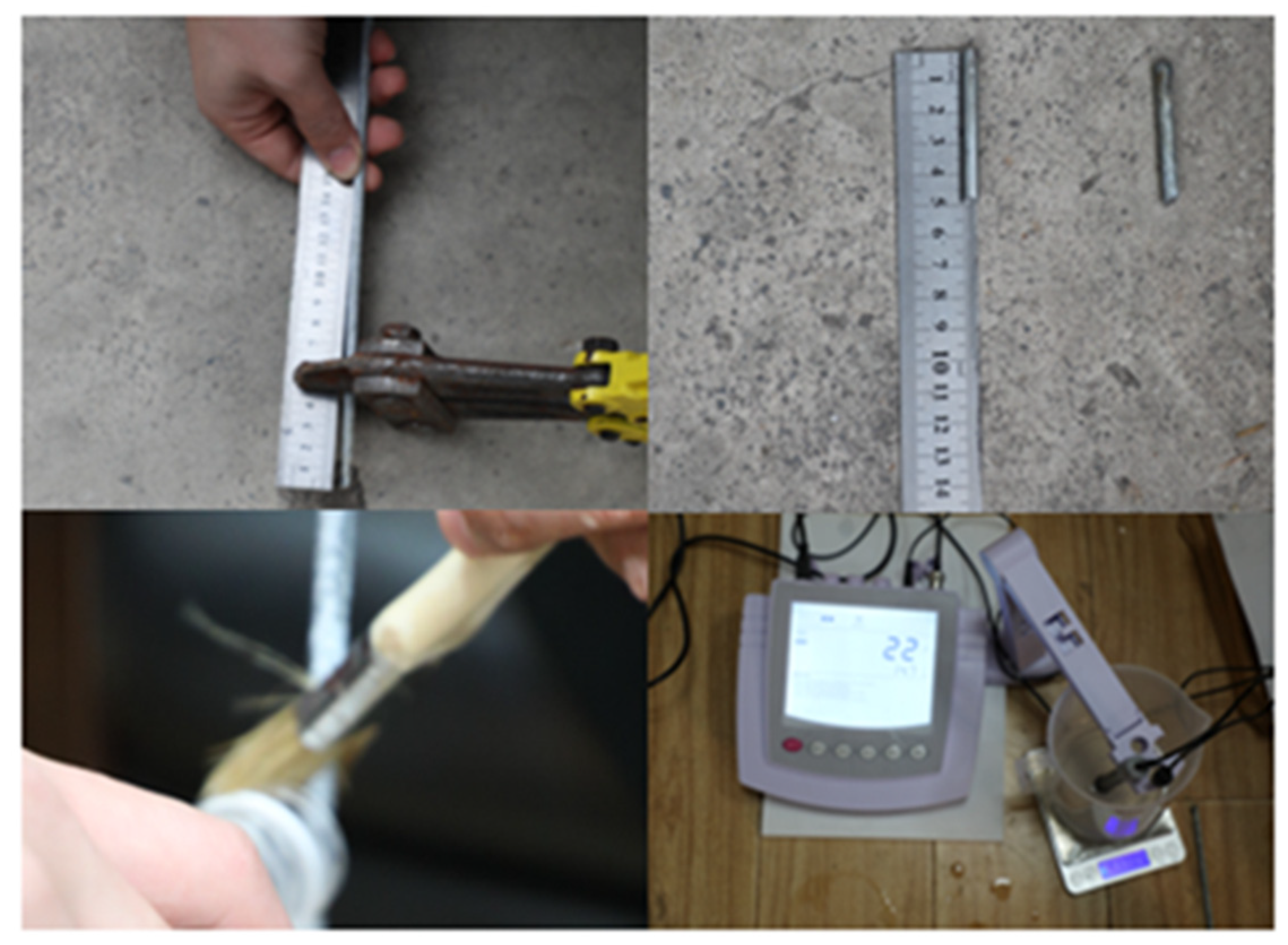
The corrosion factors diffuse from the outside to the interior of the cable due to the impact of the concentration gradient difference of corrosion factors within and outside the cable. The diffusion forms of corrosion factors in the cable can be divided into two types: (1) The corrosion factors diffuse radially along the gap between steel wires until the concentration of corrosion factors reaches saturation in each layer of steel wire on the section. (2) Corrosion factors will diffuse upwards in the longitudinal and circumferential directions of the cable due to the gaps between the layers of steel wires, eventually causing three-dimensional damage to the cable. The diffusion mechanism is shown in Figure 1.

The diffusion mechanism of corrosion factors is mainly described by Fick’s law. Fick’s law is made up of the first and second laws of Fick. Fick’s first law is proposed based on the concentration gradient difference of diffusing substances, which believes that the greater the concentration gradient difference of the diffusing substance, the greater the flow of the substance per unit of time through the unit cross-sectional area perpendicular to the direction of diffusion, proportional to the concentration gradient at the cross-section. However, Fick’s first law is only applicable to the analysis of steady-state diffusion processes, in which each volume element at any moment has an equal quantity of incoming and exiting material and a constant concentration throughout the process. This circumstance is not typical, in actuality. The diffusion of substances will be influenced by both environmental factors and the properties of the materials themselves. The diffusion rate is likely to alter as diffusion time and depth change. Based on Fick’s first law, the second law to describe the non-stationary diffusion of substances was proposed to explain the diffusion law of substances in actual processes more accurately. The law of variation of concentration of corrosion factors with diffusion time and depth was obtained. Fick’s second law can be expressed as the following equation:

$$\frac{\partial C}{\partial t}+\nabla \times \left(-D\times \nabla c\right)=0$$

(1)

where C is the concentration of corrosion factors, D is the diffusion coefficient of corrosion factors, c is the gradient difference of concentration of corrosion factors, and t is the corrosion time.

The more significant the gradient difference in concentration of corrosion factors, the faster the diffusion rate of corrosion factors, which is more likely to cause damage to parallel steel wires in the cable. For spatial diffusion issues, the concentration gradient difference of corrosion factors and the Hamiltonian operator in Equation (1) can be expressed as follows [44].

$$\left.\begin{array}{l}\nabla c=\frac{\partial C}{\partial x}+\frac{\partial C}{\partial y}+\frac{\partial C}{\partial z}\\ \nabla =\frac{\partial }{\partial x}+\frac{\partial }{\partial y}+\frac{\partial }{\partial z}\end{array}\right\}$$

(2)

By substituting Equation (2) into Equation (1), the analytical solution model of Fick’s second law’s error function can be produced, as shown below:

$$C(x,y,z)=C_0+\left(C_S-C_0\right)\left(1-erf\frac{x}{2\sqrt{D\times t}}\times erf\frac{y}{2\sqrt{D\times t}}\times erf\frac{z}{2\sqrt{D\times t}}\right)$$

(3)

where C(x,y,z) represents the concentration at any spatial point within the component, C_s is the concentration of corrosion factors on the element’s surface, C₀ is the concentration of corrosion factors within the structure, and erf is the error function.

The calculation method is shown the following equation:

$$erf\left(x\right)=\frac{2}{\sqrt{\pi }}\times {\displaystyle {\int }_0^z\exp \left({\beta }^2\right)}d\beta$$

(4)

The concentration of initial corrosion factors within the structure is relatively low in general. The effect of the concentration of corrosion factors within the structure on the predicted results is neglected to make the solution easier. Equation (3) is further simplified to obtain the following equation:

$$C(x,y,z)=C_S\times \left(1-erf\frac{x}{2\sqrt{D\times t}}\times erf\frac{y}{2\sqrt{D\times t}}\times erf\frac{z}{2\sqrt{D\times t}}\right)$$

(5)

The key to constructing a spatial diffusion model of corrosion factors, according to Equation (5), is getting the concentration and the diffusion coefficient of corrosion factors on the surface of the cable. The concentration and the diffusion coefficient of corrosion factors on the surface of the cable can be calculated using the procedures below.

The initial defect size of a square cable is shown as an example for demonstration. Create a three-dimensional coordinate system using the cable’s defect position as the center point, then characterize the cable’s damage range. Any point within the damage range can be represented as follows. Define the distance from the coordinate origin at the center position of different sampling points as R_i, as shown in Figure 2. The concentration of corrosion factors at each site is measured using electrochemical measuring equipment. After completing the test of the concentration of corrosion factors at each location of each working condition, the concentration and the diffusion coefficient of corrosion factors on the surface of the cable under various operational circumstances can be obtained by substituting results into Equation (5).

The following are the specific procedures for building the spatial diffusion model of corrosion factors using the ML method: (1) Using the testing procedures mentioned above, determine the concentration of corrosion factors at each location in the cable space along the path above. (2) Using ambient temperature, humidity, cable inclination angle, and cable defect area as input variables, the prediction model for diffusion coefficient and concentration of surface corrosion factors is created based on the ML approach. (3) According to Fick’s second law, the spatial diffusion model of corrosion factors is established by comprehensively considering the influence of environmental and material factors on the diffusion rate of corrosion factors. (4) Combine the results of the salt spray corrosion test and the prototype cable corrosion test to verify the accuracy of the prediction model.

2.2. Test Method

Due to the influence of the gradient difference of the concentration of corrosion factors inside and outside the cable, the corrosion factors diffuse from the outside to the inside. The diffusion forms of corrosion factors in the cable can be divided into two types: (1) The corrosion factors diffuse along the steel wire and the gap between the steel wires in the radial direction until the concentration of corrosion factors in each layer of the steel wire on this section reaches saturation. (2) Due to the gap between the layers of steel wires, corrosion factors will spread upward along the longitudinal and ring of the cable, resulting in three-dimensional damage to the cable. In order to clarify the diffusion law of corrosion factors in the cable, the concentration of corrosion factors on the surface of each layer of steel wire in the cable was measured by the BION-1881 chemical analyzer under different periods, defect areas, ambient temperature, and humidity. The test procedure is as follows: Firstly, the coordinate system is established with the cable defect position as the origin. Secondly, after the cable was corroded for a corresponding time, it was dissected and cut into sections of 5 cm, and its spatial position in the cable was sorted out and recorded, respectively. Finally, an electrochemical analyzer was used to measure the concentration of corrosion factors on the surface of each cut steel wire. The test procedure of the concentration of corrosion factors is as follows: (1) Each layer of corroded steel wire is processed and cut into a 5 cm section. After the processing is completed, it is numbered; (2) Wash the cut steel wire with water and repeatedly brush it with a brush to completely dissolve the corrosion factors on the surface of the steel wire in water; (3) Completely immerse one electrode rod of the electrochemical analyzer into a beaker, test the concentration of corrosion factors in the water, and take readings after stabilization to obtain the concentration of corrosion factors on the surface of the corroded steel wire. The testing process of corrosion factor concentration is shown in Figure 3. According to the test methods above, the different distribution laws of corrosion factors along the cable in radial, circumferential, and axial directions and the distribution forms of corrosion factors in three directions can be obtained, respectively.

3. Optimization of BP Neural Network Model

3.1. Data-Driven Model

The Scikit-learn software tool package is used to create five data-driven models: LR, RF, ridge regression (RR), DT, and BP neural network. The cross-validation analysis approach is used to verify the model’s accuracy to acquire the best output results. A total of 60% of the data samples (154 total) were categorized as training subsets and 40% as testing subsets (102 total) using random functions to select the training and testing sets. The following are the specific steps: To begin, split the data into groups and number them using a random function. The training and testing sets are then chosen at random. Finally, statistical performance indicators such as the decisive correlation coefficient (R²), root mean square error (RMSE), and relative root mean square error (MAE) were used to evaluate the model’s computational accuracy. R² shows the degree of fitting of the proposed model to the experimental data. R² lies between 0 and 1, and the closer its value is to the upper limit, the better the model’s fit to the experimental data. Otherwise, the worse. RMSE, commonly known as the cost function, plays a positive role in the learning process of ML algorithms. The more significant the RMSE and MAE values, the worse the model’s fitting effect on the experimental data and the lower the model’s accuracy.

Table 1. Calculation results of each data-driven model.

Mechanical Algorithm Model	R2	RMSE	MAE
BP neural network model	0.868	0.845	0.327
DT model	0.748	1.279	0.523
RF model	0.834	0.924	0.375
LR model	0.638	1.338	0.813
RR model	0.764	1.132	0.601

displays the test and verification results of various models.

As shown in Table 1, the BP neural network model has the highest R² value (0.868) from the training set, while the MAE (0.845) and RMSE (0.327) values are the lowest, indicating that the BP neural network model is most appropriate for simulating the diffusion coefficient of corrosion factors and concentration of surface corrosion factors. Similarly, the RF model’s R², RMSE, and MAE values for the testing set are 0.834, 0.924, and 0.375, respectively. The results indicate a significant correlation between the measured and predicted diffusion coefficient values of corrosion factors and the concentration of surface corrosion factors. The LR model performs the poorest, with the lowest R² (0.638) and the highest MAE (0.813). The simulation results of the diffusion coefficient of corrosion factors and the concentration of surface corrosion factors using the BP neural network are better, with the highest R² and the lowest MAE and RMSE values, as shown by the analysis findings above. The drawbacks of the BP neural network model include that it is prone to collapsing into local minima and has poor stability, which slows down the convergence speed and ultimately leads to a drop in model accuracy. As a result, updating the BP neural network model is required to increase its accuracy.

3.2. Algorithm Optimization Based on Sparrow Search Algorithm

3.2.1. Sparrow Search Algorithm

Introducing the SSA with stronger search ability and faster convergence speed to update the BP neural network to improve the accuracy of the model. The SSA is a swarm intelligence optimization algorithm that is based on the foraging and anti-predation behavior of the sparrow. The sparrow with the highest fitness is prioritized in the SSA. They are separated into discoverers and joiners during the foraging process of sparrows. Discoverers are responsible for discovering food in the population and offering foraging places and instructions for the entire sparrow population, whereas joiners rely on discoverers for food. Sparrows can usually forage as discoverers and joiners to obtain food. Individuals in the population monitor the behavior of others in the community, and attackers in this population will fight for food supplies with high-intake peers to raise their predation rate. Furthermore, when the sparrow population detects a threat, it will engage in anti-predatory behavior. During each iteration, the description of the discoverer’s location update is shown in the following equation [43]:

$${X_{i,j}}^{q+1}=\left\{\begin{array}{l}{X_{i,j}}^q\exp \left(\frac{-i}{\alpha \times ite{r}_{\max }}\right),if\hspace{1em}{R}_2\le ST\\ {X_{i,j}}^q+Q\times L,if\hspace{1em}{R}_2>ST\end{array}\right.$$

(6)

where q is the current number of iterations, iter_max is the largest iteration algebra, X_ij is the position information of the i-th sparrow in the j-th dimension, α is the random number(α ∈ (0, 1]), R₂ is the warning value (R₂ ∈ [0, 1]), ST is the safety value (ST ∈ [0.5, 1]), Q is the random number subject to normal distribution, and L is a matrix of 1 × d, where each element within the matrix is all 1.

When R₂ < ST, it indicates that there are no predators in the foraging environment, allowing for the discoverers to conduct lengthy search activities. If R₂ ≥ ST, it means that some sparrows in the population have detected predators and alerted other sparrows. At this time, the sparrows must fly immediately to other safe areas for feeding. The description of the joiner’s location update is shown in the following equation:

$${X_{i,j}}^{q+1}=\left\{\begin{array}{l}{X_{best}}^q+\beta \times \left|{X_{i,j}}^q-\left.{X_{best}}^q\right|,\right.if\hspace{1em}{f}_i>f_g\\ {X_{i,j}}^{q+1}+K\times \left(\frac{{X_{i,j}}^q-{X_{worst}}^q}{\left(f_i-f_w\right)+\epsilon }\right),if\hspace{0.17em}\begin{array}{c}{f}_i=f_g\end{array}\end{array}\right.$$

(7)

where X_best is the optimal position occupied by the discoverer; X_worst is the current global position; β is the control parameter of step size, which follows the normal distribution random number with the mean of 0 and variance of 1; K ∈ [−1, 1] represents the random number; f_i is the fitness value of current sparrow individuals; f_g is the fitness value of the sparrow in the current global optimal position; f_w is the fitness value of the sparrow in the current global worst position; and ε is a constant.

Among these, f_i > f_g indicates that sparrows are on the periphery of the population and highly vulnerable to predators. When f_i = f, it demonstrates that sparrows in the middle of the population know the danger and should approach other sparrows to reduce the predation risk. K controls the direction of the sparrow’s movement and step size.

3.2.2. Optimization of BP Neural Network Algorithm

During the calculation process, the selection of the number of neurons in the hidden layer significantly impacts the model’s calculation accuracy and speed. The more neurons in the hidden layer, the higher the model’s accuracy, but the slower the computation speed. On the contrary, the smaller the number of neurons, the lower the computational accuracy of the model, but the faster the model operates. As a result, it is critical to reasonably determine the number of neurons in the hidden layer, which not only preserves a certain accuracy in the model but also increases its computational speed. According to the relevant literature [32], the number of neurons in the model can be calculated using the following formula:

$$Q=\sqrt{M+N}+A$$

(8)

where Q is the number of neurons in the hidden layer, M is the number of neurons in the input layer, N is the number of neurons in the output layer, and A is an integer between 1 and 10.

Considering the influence of overfitting and underfitting, after repeated debugging, Q is 10, and the test accuracy of the model is the highest. The calculation process of the entire model is shown in Figure 4.

Figure 5 and Figure 6 demonstrate the prediction results of the SSA-BP neural network and the BP neural network. Figure 7 and Figure 8 show that the SSA-BP model has a high R² (0.93) and the lowest RMSE (0.0378), which indicates that the updated model can accurately forecast the concentration of surface corrosion factors and the diffusion coefficient of corrosion factors. In addition, BP requires 13 iterations to achieve convergence, whereas the SSA-BP model only requires 9 iterations, indicating a significant improvement in the convergence speed of the SSA-BP model. The model was trained and simulated 20 times to compare the robustness of the SSA-BP model with the BP model, and the results are shown in Figure 9. The coefficient of variation of the SSA-BP model was found to be between 5% and 18%, whereas the coefficient of variation of the BP model was between 7% and 35%.

4. Analysis of Parameter Sensitivity

The SSA-BP neural network model was used to calculate the weights between the input and hidden layer to analyze the impact of various parameters on the diffusion coefficient D of corrosion factors and the concentration Cs of surface corrosion factors. The results are shown in

Table 2. Results of connection weights for the input and hidden layer.

Hidden Layer	Defect Size	Dip Angle	Temperature	Humidity	Corrosion Time	Deviation
B1	−0.06	−0.14	−0.38	−0.15	0.12	0.05
B2	−0.35	0.92	0.27	0.31	0.87	0.08
B3	−0.72	−0.23	−0.01	−0.34	−0.15	−0.65
B4	0.25	0.14	0.52	−0.22	−0.05	−0.53
B5	0.52	−0.25	0.12	0.64	−0.05	−0.27
B6	−0.23	0.08	0.38	−0.59	0.07	0.42
B7	−0.36	0.17	−0.27	−0.19	−0.34	0.28
B8	0.54	−0.09	−0.32	0.65	−0.58	−0.47
B9	0.47	−0.51	−0.33	−1.04	0.85	−0.02
B10	−0.72	0.23	−0.47	0.58	0.09	−0.41

and

Table 3. Weight values of the hidden and output layer.

B1	B2	B3	B4	B5	B6	B7	B8	B9	B10	Bias
−0.53	0.41	0.36	0.54	−0.47	−0.38	−1.22	1.08	0.17	0.41	0.62

, respectively.

The Garson formula was used to calculate the significant impacts of input parameters on the transfer coefficient of corrosion factors and the concentration of surface corrosion factors, as indicated in the following equation:

$$Z_{ik}=\frac{{\displaystyle \sum _{j=1}^L\left(\frac{w_{ij}}{{\displaystyle \sum _{r=1}^N{w}_{rj}}}{v}_{jk}\right)}}{{\displaystyle \sum _{i=1}^N\left({\displaystyle \sum _{j=1}^L\left(\frac{w_{ij}}{{\displaystyle \sum _{r=1}^N{w}_{rj}}}{v}_{jk}\right)}\right)}}$$

(9)

where w_rj is the connection weight value between the input neuron and the hidden layer neuron j, and v_jk is the connection weight value between the hidden layer neuron j and the output neuron K.

The impact of input parameters on the concentration of surface corrosion factors and diffusion coefficient of corrosion factors can be obtained using the steps above based on the connection weights value and biases between the input, hidden, and output layers. The results are shown in Figure 10.

Figure 10 depicts the impact of various parameters on the concentration of surface corrosion factors and the transfer coefficient of corrosion factors. The results demonstrate that the dip angle and the defect area of the cable have the most significant effect on both, with weight values all greater than 0.25. Although environmental temperature, humidity, and corrosion time all impact the diffusion rate of corrosion factors, their weight values are all within 0.2. According to the results of the weight analysis of the SSA-BP neural network model, the concentration of surface corrosion factors and diffusion coefficient of corrosion factors of the cable above the defect location (A1 segment cable) and the cable below the defect location (B1 segment cable) were fitted using the tilt angle of cables by the distinguishing criterion, and were based on multiple nonlinear regression criteria. The fitting equation for the concentration of surface corrosion factors and the diffusion coefficient of corrosion factors on the A1 segment cable is shown in the following equation:

$$\left.\begin{array}{l}{C}_s=\alpha ·{\left(t\right)}^{A_1}·{\left(h\right)}^{A_2}·{\left(T_1\right)}^{A_3}{\left(W\right)}^{A_4}·{\left(\cos \theta \right)}^{A_5}+H\\ D=\left[\beta ·{\left(t\right)}^{B_1}·{\left(h\right)}^{B_2}·{\left(T_1\right)}^{B_3}{\left(W\right)}^{B_4}·{\left(\cos \theta \right)}^{B_5}+Q\right]\times {10}^{-10}\end{array}\right\}$$

(10)

Referring to Equation (10), according to the difference between the concentration of surface corrosion factors and the diffusion coefficient of corrosion factors on the A1 and B1 cable sections, the concentration of surface corrosion factors and the diffusion coefficient of corrosion factors on the B1 cable section can be expressed as the following equation:

$$\left.\begin{array}{l}{C}_s={\eta }_1\left[\alpha ·{\left(t\right)}^{A_1}·{\left(h\right)}^{A_2}·{\left(T_1\right)}^{A_3}{\left(W\right)}^{A_4}·{\left(\cos \theta \right)}^{A_5}+H\right]\\ D=\eta \left[\beta ·{\left(t\right)}^{B_1}·{\left(h\right)}^{B_2}·{\left(T_1\right)}^{B_3}{\left(W\right)}^{B_4}·{\left(\cos \theta \right)}^{B_5}+Q\right]\times {10}^{-10}\end{array}\right\}$$

(11)

where t is the corrosion time of the cable, h is the relative humidity of the environment, T₁ is the ambient temperature, W is the defect size area, θ is the dip angle of the cable, and A₁–A₅, B₁–B₅, H and Q are undetermined parameters.

MATLAB software programming was used to calculate Equation (10) and bring the known parameters into Equation (10) based on the nonlinear regression function to calculate the concentration of surface corrosion factors and diffusion coefficient of corrosion factors on the cable under different working conditions. The expression of the concentration of surface corrosion factors and the diffusion coefficient of corrosion factors on the A1 segment cable is as follows:

$$\left.\begin{array}{l}{C}_s=0.387·{\left(t\right)}^{0.32}·{\left(h\right)}^{0.08}·{\left(T_1\right)}^{0.12}{\left(W\right)}^{0.52}·{\left(\cos \theta \right)}^{0.43}+0.216\\ D=\left[11.42·{\left(t\right)}^{0.23}·{\left(h\right)}^{0.05}·{\left(T_1\right)}^{0.11}{\left(W\right)}^{0.54}·{\left(\cos \theta \right)}^{0.41}+1.231\right]\times {10}^{-10}\end{array}\right\}$$

(12)

The diffusion rate of corrosion factors differs between the A1 and B1 segment cables due to the inclination of the cable. The diffusion rate is faster in the B1 section of the cable but slower in the A1 section. According to Equation (12), the expression of the concentration of surface corrosion factors and the diffusion coefficient of corrosion factors on the B1 segment cable is as follows:

$$\left.\begin{array}{l}{C}_s={\eta }_1\left[0.387·{\left(t\right)}^{0.32}·{\left(h\right)}^{0.08}·{\left(T_1\right)}^{0.12}{\left(W\right)}^{0.52}·{\left(\cos \theta \right)}^{0.43}+0.216\right]\\ D=\eta \left[11.42·{\left(t\right)}^{0.23}·{\left(h\right)}^{0.05}·{\left(T_1\right)}^{0.11}{\left(W\right)}^{0.54}·{\left(\cos \theta \right)}^{0.41}+1.231\right]\times {10}^{-10}\end{array}\right\}$$

(13)

The values of η₁ and η under different tilt angles based on the differences in the concentrations of corrosion factors between different layers inside the A1 and B1 cable segments are shown in

Table 4. The range of values of η₁ and η under different tilt angles.

Tilt Angle	η1	η
0	1.02	1.01
30	0.92	1.12
45	0.85	1.18
60	0.72	1.26

.

Table 4 shows that when the inclination of the cable increases, the concentration of surface corrosion factors on the B1 cable section gradually decreases compared to the A1 cable section. However, the diffusion coefficient of corrosion factors follows the reverse law, with the diffusion coefficient of corrosion factors on the B1 cable segment being significantly greater than that on the A1 cable section, which indicates that the diffusion rate of corrosion factors downward along the cable’s inclination angle is more significant than that upward along the cable’s inclination angle. This phenomenon is caused by the following: as the cable’s inclination increases, substances such as water, corrosion factors, and oxygen travel lower along the cable, and the corrosion factors continually penetrate from the surface to the interior. As a result, the concentration of surface corrosion factors in section B1 is low, and the diffusion coefficient of corrosion factors is large. The gravity effect will obstruct the upward diffusion of corrosion factors and other substances along the A1 cable segment, resulting in the aggregation of corrosion factors on the cable surface and a decrease in the diffusion coefficient of corrosion factors.

The above depicts the process of solving the concentration of surface corrosion factors and diffusion coefficient of corrosion factors on square-hole defect cable. The diffusion form of corrosion factors in the annular hole cable is studied using the analysis method described above. The spatial diffusion model of corrosion factors in the annular hole defect cable is built to obtain the expression of the concentration of surface corrosion factors and the diffusion coefficient of corrosion factors. It can still be separated into two segments for convenience of representation: the C1 segment above the defect location and the D1 segment below the defect location. The expression is as follows.

(1)

The expression of concentration of surface corrosion factors and diffusion coefficient of corrosion factors in the C1 cable segment:

$$\left.\begin{array}{l}{C}_s=0.393·{\left(t\right)}^{0.24}·{\left(h\right)}^{0.12}·{\left(T_1\right)}^{0.16}{\left(W\right)}^{0.57}·{\left(\cos \theta \right)}^{0.46}+0.413\\ D=\left[13.32·{\left(t\right)}^{0.26}·{\left(h\right)}^{0.06}·{\left(T_1\right)}^{0.13}{\left(W\right)}^{0.63}·{\left(\cos \theta \right)}^{0.47}+1.572\right]\times {10}^{-10}\end{array}\right\}$$

(14)

According to the expression method of the concentration of surface corrosion factors and diffusion coefficient of corrosion factors on the C1 cable section, the concentration of surface corrosion factors and diffusion coefficient of corrosion factors on the D1 cable section can be expressed as follows.

$$\left.\begin{array}{l}{C}_s={\eta }_2\left[0.393·{\left(t\right)}^{0.24}·{\left(h\right)}^{0.12}·{\left(T_1\right)}^{0.16}{\left(W\right)}^{0.57}·{\left(\cos \theta \right)}^{0.46}+0.413\right]\\ D={\eta }_3\left[13.32·{\left(t\right)}^{0.26}·{\left(h\right)}^{0.06}·{\left(T_1\right)}^{0.13}{\left(W\right)}^{0.63}·{\left(\cos \theta \right)}^{0.47}+1.572\right]\times {10}^{-10}\end{array}\right\}$$

(15)

Table 5. The range of values of η₂ and η₃ under different tilt angles.

Tilt Angle	η2	η3
0	1.04	1.02
30	0.89	1.17
45	0.81	1.22
60	0.68	1.35

shows the values of η₂ and η₃ at different tilt angles. The amplification coefficients of the concentration of surface corrosion factors and diffusion coefficients of corrosion factors on the D1 segment cable under tilt angles are shown in Table 5. Compared with the results shown in Table 4, the tilt angle has a more significant impact on the concentration of surface corrosion factors and diffusion coefficient of corrosion factors on the ring defect cable.

5. Spatial Diffusion Model of Corrosion Factors

Based on the analysis results above, the spatial diffusion model of corrosion factors in the cable can be established under various tilt angles, temperatures, humidity, corrosion periods, and defect areas, divided into upper and lower cable sections for display. Firstly, the spatial diffusion model of corrosion factors in the square hole defective cable is exhibited. The results are shown below.

(1)

The spatial diffusion model of corrosion factors in the A1 cable segment.

$$\left.\begin{array}{l}{C}_s=0.387·{\left(t\right)}^{0.32}·{\left(h\right)}^{0.08}·{\left(T_1\right)}^{0.12}{\left(W\right)}^{0.52}·{\left(\cos \theta \right)}^{0.43}+0.216\\ D=\left[11.42·{\left(t\right)}^{0.23}·{\left(h\right)}^{0.05}·{\left(T_1\right)}^{0.11}{\left(W\right)}^{0.54}·{\left(\cos \theta \right)}^{0.41}+1.231\right]\times {10}^{-10}\\ C(x,y,z)=C_S\times \left(1-erf\frac{x}{2\sqrt{D\times t}}\times erf\frac{y}{2\sqrt{D\times t}}\times erf\frac{z}{2\sqrt{D\times t}}\right)\end{array}\right\}$$

(16)

(2)

The spatial diffusion model of corrosion factors in the B1 cable segment.

$$\left.\begin{array}{l}{C}_s={\eta }_1\left[0.387·{\left(t\right)}^{0.32}·{\left(h\right)}^{0.08}·{\left(T_1\right)}^{0.12}{\left(W\right)}^{0.52}·{\left(\cos \theta \right)}^{0.43}+0.216\right]\\ D=\eta \left[11.42·{\left(t\right)}^{0.23}·{\left(h\right)}^{0.05}·{\left(T_1\right)}^{0.11}{\left(W\right)}^{0.54}·{\left(\cos \theta \right)}^{0.41}+1.231\right]\times {10}^{-10}\\ C(x,y,z)=C_S\times \left(1-erf\frac{x}{2\sqrt{D\times t}}\times erf\frac{y}{2\sqrt{D\times t}}\times erf\frac{z}{2\sqrt{D\times t}}\right)\end{array}\right\}$$

(17)

Among them, the values of η₁ and η under different tilt angles are shown in Table 5. The spatial diffusion model of corrosion factors within the annular defect cable can be depicted as follows using the approach described above.

(1)

The spatial diffusion model of corrosion factors in the C1 cable segment.

$$\left.\begin{array}{l}{C}_s=0.393·{\left(t\right)}^{0.24}·{\left(h\right)}^{0.12}·{\left(T_1\right)}^{0.16}{\left(W\right)}^{0.57}·{\left(\cos \theta \right)}^{0.46}+0.413\\ D=\left[13.32·{\left(t\right)}^{0.26}·{\left(h\right)}^{0.06}·{\left(T_1\right)}^{0.13}{\left(W\right)}^{0.63}·{\left(\cos \theta \right)}^{0.47}+1.572\right]\times {10}^{-10}\\ C(x,y,z)=C_S\times \left(1-erf\frac{x}{2\sqrt{D\times t}}\times erf\frac{y}{2\sqrt{D\times t}}\times erf\frac{z}{2\sqrt{D\times t}}\right)\end{array}\right\}$$

(18)

(2)

The spatial diffusion model of corrosion factors in the D1 cable segment.

$$\left.\begin{array}{l}{C}_s={\eta }_2\left[0.393·{\left(t\right)}^{0.24}·{\left(h\right)}^{0.12}·{\left(T_1\right)}^{0.16}{\left(W\right)}^{0.57}·{\left(\cos \theta \right)}^{0.46}+0.413\right]\\ D={\eta }_3\left[13.32·{\left(t\right)}^{0.26}·{\left(h\right)}^{0.06}·{\left(T_1\right)}^{0.13}{\left(W\right)}^{0.63}·{\left(\cos \theta \right)}^{0.47}+1.572\right]\times {10}^{-10}\\ C(x,y,z)=C_S\times \left(1-erf\frac{x}{2\sqrt{D\times t}}\times erf\frac{y}{2\sqrt{D\times t}}\times erf\frac{z}{2\sqrt{D\times t}}\right)\end{array}\right\}$$

(19)

Among them, Table 5 shows the values of η₂ and η₃ under various tilt angles. The concentration of corrosion factors at each spatial position of the cable was calculated using this model to verify the accuracy of the model above. The calculated results were compared with the measured results, as shown in Figure 11, Figure 12, Figure 13 and Figure 14. The findings demonstrate that the prediction results of the model are lower than the experimental test results, and the relative error between the two is within 15%, illustrating that the prediction model proposed in this article has a certain accuracy.

6. Conclusions

The spatial diffusion model of corrosion factors was built using the ML method based on the test results of concentrations of corrosion factors at various positions in the space of the cable system and Fick’s second law. The relevant empirical formulae were presented, and the accuracy of the theoretical model was verified using multiple nonlinear regression analysis methods, taking into account the effect of various parameters on the diffusion coefficient of corrosion factors and the concentration of surface corrosion factors. The specific conclusions are as follows:

(1)

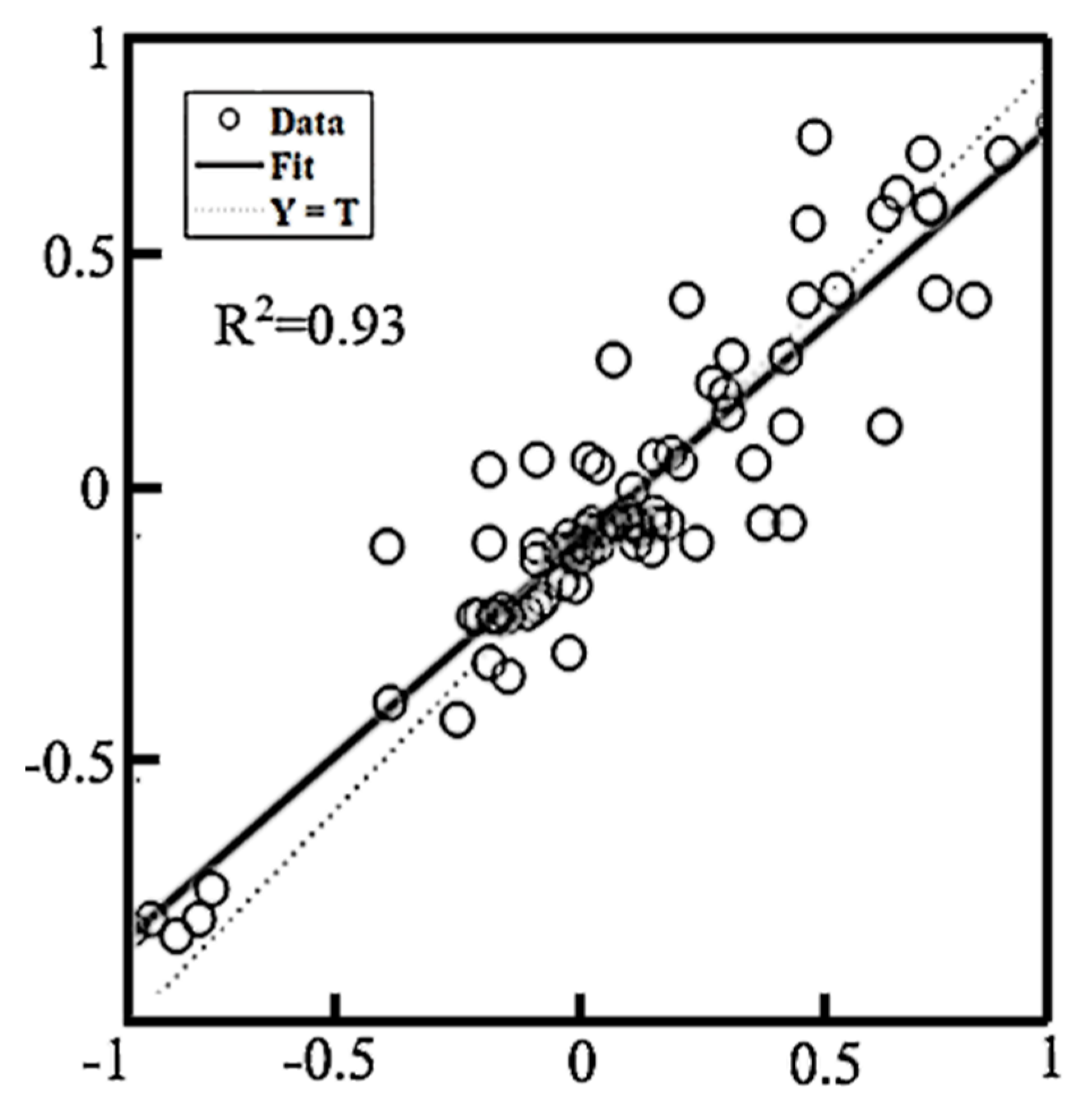
Five ML algorithms were used to investigate the impacts of environmental temperature, humidity, cable inclination angle, and cable defect size on the diffusion coefficient of corrosion factors and the concentration of surface corrosion factors. According to the simulation findings, the optimized BP neural network method has the best simulation effect, with fast convergence speed and good robustness.

(2)

The inclination angle and the defect size of the cable are the primary parameters influencing the diffusion coefficient of corrosion factors and the concentration of surface corrosion factors—their weight values are all above 0.25. Although environmental temperature, humidity, and corrosion time all affect the diffusion rate of corrosion factors, they are more limited, and their weight values are all within 0.2.

(3)

Due to the increase in the inclination of the cable, substances such as water, corrosion factors, and oxygen will move downwards along the cable, and corrosion factors will continually penetrate from the surface to the interior of the cable. The concentration of surface corrosion factors on the cable above the defect is low, and the diffusion coefficient of corrosion factors is high. The gravity effect will impede the upward diffusion of corrosion factors and other substances along the cable, resulting in the aggregation of corrosion factors on the surface of the cable below the defect and a drop in the diffusion coefficient of corrosion factors.

(4)

The cross-sectional loss or corrosion weight loss of the steel wire inside the cable mainly occurs where corrosion factors gather. The area with the highest concentration of corrosion factors is the area where corrosion occurs most severely. The diffusion path of corrosion factors is the area where corrosion is most likely to occur during the service process of the cable. Studying the diffusion trend of corrosion factors can provide guidance for the corrosion protection of steel wires in different parts. The concentration of corrosion factors at each spatial position of the cable was calculated using the model in this article. The predicted results of the spatial diffusion model of cable were lower than the measured results of the experiment, with a relative error of 15%, showing a good level of agreement, which can effectively forecast and assess the spatial diffusion status of cable’s corrosion factors in practical engineering.

References

1. Liu, Z.; Guo, T.; Huang, L.; Pan, Z. Fatigue life evaluation on short suspenders of long-span suspension bridge with central clamps. J. Bridge Eng. 2017, 22, 04017074. [Google Scholar] [CrossRef]
2. Morcous, G.; Lounis, Z.; Cho, Y. An integrated system for bridge management using probabilistic and mechanistic deterioration models: Application to bridge decks. KSCE J. Civ. Eng. 2010, 14, 527–537. [Google Scholar] [CrossRef]
3. Zheng, G.; Tang, W.; Wang, P. Bridge Cable Structures; China Communications Press: Beijing, China, 2015. [Google Scholar]
4. Aloisio, A.; Pasca, D.P.; Rosso, M.M.; Briseghella, B. Role of cable forces in the model updating of cable-stayed bridges. J. Bridge Eng. 2023, 28, 05023002. [Google Scholar] [CrossRef]
5. Greco, F.; Lonetti, P.; Pascuzzo, A. Dynamic Analysis of Cable-Stayed Bridges Affected by Accidental Failure Mechanisms under Moving Loads. Math. Probl. Eng. 2013, 2013, 302706. [Google Scholar] [CrossRef] [Green Version]
6. Ammendolea, D.; Bruno, D.; Greco, F.; Lonetti, P.; Pascuzzo, A. An investigation on the structural integrity of network arch bridges subjected to cable loss under the action of moving loads. Procedia Struct. Integr. 2020, 25, 305–315. [Google Scholar] [CrossRef]
7. Mozos, C.M.; Aparicio, A.C. Parametric study on the dynamic response of cable stayed bridges to the sudden failure of a stay, Part I: Bending moment acting on the deck. Eng. Struct. 2010, 32, 3288–3300. [Google Scholar] [CrossRef]
8. Mozos, C.M.; Aparicio, A.C. Parametric study on the dynamic response of cable stayed bridges to the sudden failure of a stay, Part II: Bending moment acting on the pylons and stress on the stays. Eng. Struct. 2010, 32, 3301–3312. [Google Scholar] [CrossRef]
9. Qiao, Y.; Miao, C.; Sun, C. Evaluation of corrosion fatigue life for corroded wire for cable-supported bridge. J. Civ. Environ. Eng. 2017, 39, 115–121. [Google Scholar]
10. Stewart, M.G.; Al-Harthy, A. Pitting corrosion and structural reliability of corroding RC structures: Experimental data and probabilistic analysis. Reliab. Eng. Syst. Saf. 2006, 93, 373–382. [Google Scholar] [CrossRef]
11. Li, R.; Miao, C.; Wei, T. Experimental study on corrosion behavior of galvanized steel wires under stress. Corros. Eng. Sci. Technol. 2020, 55, 622–633. [Google Scholar] [CrossRef]
12. Miao, C.; Yu, J.; Mei, M. Distribution law of corrosion pits on steel suspension wires for a tied arch bridge. Anti-Corros. Methods Mater. 2016, 63, 166–170. [Google Scholar] [CrossRef]
13. Betti, R.; West, A.C.; Vermaas, G.; Cao, Y. Corrosion and embrittlement in high-strength wires of suspension bridge cables. J. Bridge Eng. 2005, 10, 151–162. [Google Scholar] [CrossRef]
14. Furuya, K.; Kitagawa, M.; Nakamura, S.I.; Suzumura, K. Corrosion mechanism and protection methods for suspension bridge cables. Struct. Eng. Int. 2000, 10, 189–193. [Google Scholar] [CrossRef]
15. Suzumura, K.; Nakamura, S.I. Environmental factors affecting corrosion of galvanized steel wires. J. Mater. Civ. Eng. 2004, 16, 1–7. [Google Scholar] [CrossRef]
16. Nakamura, S.I.; Suzumura, K. Hydrogen embrittlement and corrosion fatigue of corroded bridge wires. J. Constr. Steel Res. 2008, 65, 269–277. [Google Scholar] [CrossRef]
17. Sloane, M.J.D.; Betti, R.; Marconi, G.; Hong, A.L.; Khazem, D. Experimental analysis of a nondestructive corrosion monitoring system for main cables of suspension bridges. J. Bridge Eng. 2013, 18, 653–662. [Google Scholar] [CrossRef]
18. Zin, I.M.; Howard, R.L.; Badger, S.J.; Scantlebury, J.D.; Lyon, S.B. The mode of action of chromate inhibitor in epoxy primer on galvanized steel. Prog. Org. Coat. 1998, 33, 203–210. [Google Scholar] [CrossRef]
19. Yao, G.; Yang, S.; Zhang, J.; Leng, Y. Analysis of corrosion-fatigue damage and fracture mechanism of in-service bridge cables/hangers. Adv. Civ. Eng. 2021, 2021, 6633706. [Google Scholar]
20. Yang, S.; Yao, G.; Zhang, J.; Shi, K. The corrosion fatigue characteristic of steel strand experiencing an artificial accelerated salt fog aging. Mater. Rep. 2018, 32, 1988–1993. [Google Scholar]
21. Qin, H.; Shen, Q.; Ou, J.; Zhu, W. Long-term monitoring reliability and life prediction of fiber bragg grating-based self-sensing steel strands. Adv. Civ. Eng. 2020, 2020, 7687039. [Google Scholar] [CrossRef]
22. Furuya, T.; Kawafuku, J.; Satoh, H.; Shimogori, K.; Aoshima, A.; Takeda, S. A corrosion testing method for titanium in nitric acid environments. ISIJ Int. 1991, 31, 189–193. [Google Scholar] [CrossRef]
23. Hamilton, H.R., III. Bridge stay cable corrosion protection. I: Grout injection and load testing. J. Bridge Eng. 1998, 3, 64–71. [Google Scholar] [CrossRef]
24. Hamilton, H.R., III; Breen, J.E.; Frank, K.H. Bridge stay cable corrosion protection. II: Accelerated corrosion tests. J. Bridge Eng. 1998, 3, 72–81. [Google Scholar] [CrossRef]
25. Matsumoto, M.; Yagi, T.; Shigemura, Y.; Tsushima, D. Vortex-induced cable vibration of cable-stayed bridges at high reduced wind velocity. J. Wind. Eng. Ind. Aerodyn. 2001, 89, 633–647. [Google Scholar] [CrossRef]
26. Wu, Z.; Ding, Z.; Sun, C.; Zhang, L. Finite element analysis of section stress and failure mode of steel strand. China Sci. 2018, 13, 2623–2628. [Google Scholar]
27. Wang, X.; Wang, J.; Jin, M.; Yang, C. Analysis of coupling injury caused by corrosion and fatigue of fable stayed cables. J. Taiyuan Univ. Sci. Technol. 2019, 40, 472–476. [Google Scholar]
28. Yang, S.; Zhang, J.; Yao, G. Analysis on corrosion-fatigue damage and fracture mechanism of cables /hangers in service bridges. J. Highw. Transp. Res. Dev. 2019, 36, 80–86. [Google Scholar]
29. Guo, Z.; Li, L.; Yao, G. Corrosion behavior analysis of wire-steel in cables and its prediction under combined effect of cycling loading and eroded environment. J. Chongqing Univ. 2018, 41, 48–57. [Google Scholar]
30. Rosso, M.M.; Asso, R.; Aloisio, A.; Di, B.M.; Cucuzza, R.; Greco, R. Corrosion effects on the capacity and ductility of concrete half-joint bridges. Constr. Build. Mater. 2022, 360, 129555. [Google Scholar] [CrossRef]
31. Li, S.; Xin, J.; Jiang, Y.; Wang, C.; Zhou, J.; Yang, X. Temperature-induced deflection separation based on bridge deflection data using the TVFEMD-PE-KLD method. J. Civ. Struct. Health Monit. 2023, 13, 781–797. [Google Scholar] [CrossRef]
32. Xin, J.; Jiang, Y.; Zhou, J.; Peng, L.; Liu, S.; Tang, Q. Bridge deformation prediction based on SHM data using improved VMD and conditional KDE. Eng. Struct. 2022, 261, 114285. [Google Scholar] [CrossRef]
33. Xin, J.; Zhou, C.; Jiang, Y.; Tang, Q.; Yang, X.; Zhou, J. A signal recovery method for bridge monitoring system using TVFEMD and encoder-decoder aided LSTM. Measurement 2023, 214, 112797. [Google Scholar] [CrossRef]
34. Kim, D.S.; Lee, H.S.; Lee, S.M.; Wang, X.Y. A study on the evaluation of probabilistic durability life for RC structures deteriorated by chloride ion. Key Eng. Mater. 2007, 76, 417–420. [Google Scholar] [CrossRef]
35. Gupta, T.; Patel, K.A.; Siddique, S.; Sharma, R.K.; Chaudhary, S. Prediction of mechanical properties of rubberized concrete exposed to elevated temperature using ANN. Measurement 2019, 147, 106870. [Google Scholar] [CrossRef]
36. Yu, Y.; Zhao, X.; Xu, J.; Wang, S.; Xie, T. Evaluation of shear capacity of steel fiber reinforced concrete beams without stirrups using artificial intelligence models. Materials 2022, 15, 2407. [Google Scholar] [CrossRef]
37. Bukhsh, Z.A.; Stipanovic, I.; Saeed, A.; Doree, A.G. Maintenance intervention predictions using entity-embedding neural networks. Autom. Constr. 2020, 116, 103202. [Google Scholar] [CrossRef]
38. Miao, P. Prediction-based maintenance of existing bridges using neural network and sensitivity analysis. Adv. Civ. Eng. 2021, 2021, 4598337. [Google Scholar] [CrossRef]
39. Cao, B. An Improved Decision Tree Algorithm Based on Density. Master’s Thesis, Dalian University of Technology, Dalian, China, 2016. [Google Scholar]
40. Qiao, P.; Liang, Z.; Xu, K.; Zhong, C.; Qin, F. Evaluation of technical condition of medium and small span bridge based on machine learning. J. Chang. Univ. (Nat. Sci. Ed.) 2021, 41, 39–52. [Google Scholar]
41. Wu, D.; Liu, L.; Miao, R. Neural network method in bridge condition assessment by B-TBU model. J. Jiangsu Univ. (Nat. Sci. Ed.) 2017, 38, 466–471. [Google Scholar]
42. Li, Y.; Zou, Z.; Xu, L.; Wang, Y. Risk assessment study of decision tree analysis technology during bridge construction. J. China Foreign Highw. 2019, 39, 297–302. [Google Scholar]
43. Yang, S. Research on maximum power point tracking of photovoltaic system based on sparrow search algorithm to optimize BP neural network. Sci. Technol. Innov. 2022, 16, 62–63, 66. [Google Scholar]
44. Ju, X.; Wu, L.; Liu, M.; Zhang, H.; Li, T. Service life prediction for reinforced concrete wharf considering the influence of chloride erosion dimension. Mater. Rep. 2021, 35, 24075–24080, 24087. [Google Scholar]
Figure 1. Transfer form of corrosion factors in the cable: (a) radial transmission; (b) circular and axial transmission.
Buildings 13 01485 g001
Figure 2. Schematic diagram of sampling points for corrosion factors.
Buildings 13 01485 g002
Figure 3. Testing process of corrosion factor concentration.
Buildings 13 01485 g003
Figure 4. Process of the SSA-BP model.
Buildings 13 01485 g004
Figure 5. Prediction results of the SSA-BP model.
Buildings 13 01485 g005
Figure 6. Prediction results of the BP model.
Buildings 13 01485 g006
Figure 7. Convergence process of the BP model.
Buildings 13 01485 g007
Figure 8. Convergence process of the SSA-BP model.
Buildings 13 01485 g008
Figure 9. Analysis results of robustness of the SSA-BP and BP model.
Buildings 13 01485 g009
Figure 10. Weight analysis results of each input parameter on the corrosion factor of cable. (a) Concentration of surface corrosion factors; (b) Transfer coefficient of corrosion factors.
Buildings 13 01485 g010
Figure 11. Comparison results of the A1 segment cable (defect size is 2 cm × 2 cm): (a) tilt angle 30°; (b) tilt angle 45°.
Buildings 13 01485 g011
Figure 12. Comparison results of the B1 segment cable (defect size is 2 cm × 2 cm): (a) tilt angle 30°; (b) tilt angle 45°.
Buildings 13 01485 g012
Figure 13. Comparison results of the C1 segment cable (defect size width is 3 cm): (a) tilt angle 0°; (b) tilt angle 30°.
Buildings 13 01485 g013
Figure 14. Comparison results of the D1 segment cable (defect size width is 3 cm): (a) tilt angle 0°; (b) tilt angle 30°.
Buildings 13 01485 g014