Theoretical and Numerical Examination of a Novel Method for Identifying Bridge Moving Force Using an Instrumented Vehicle

Abstract

This study presents a novel and highly efficient technique to identify moving forces by utilising the acceleration response of an instrumented moving vehicle. The complex task of determining moving forces is transformed into one of solving linear equations, made easier through the Newmark-β method. To overcome the ill-conditioned problem and improve the recognition accuracy, Tikhonov regularisation is employed. Uniquely, this approach necessitates the placement sensors on the vehicle alone to record the responses of the vehicle–bridge coupled system as it traverses the bridge. Once the coupled responses are acquired, the moving force is quickly identified using the proposed method. The reliability of this method is numerically verified using a case study of a single degree-of-freedom vehicle crossing a simply supported beam. The performance of the proposed method is further demonstrated by examining several typical external factors. The results indicate that the method presents a high recognition accuracy, demonstrating good robustness and reliability even amidst substantial environmental noise interference. This proposed method offers a new perspective for identifying the moving force of small- to medium-span bridges.

1. Introduction

The installation of structural health monitoring systems (SHMSs) has emerged as an effective approach with which to gauge bridge responses, detect potential damage, and evaluate the overall condition of bridges [1,2]. To date, numerous SHMSs comprising a multitude of sensors have been set up on a range of modern bridges, notably the Qingma bridge and the Hong Kong–Zhuhai–Macao bridge [1]. Such systems accumulate extensive data during the operational phase of these structures. The data amassed are analysed using various data-driven assessment algorithms, including machine learning, deep learning, and other intelligence approaches, which are proposed based on the dataset recorded via the SHMS [3]. These data-driven algorithms aid in the extraction of crucial features’ parameters to evaluate the health condition of bridges. Despite the SHMS’s capability in detecting anomalies in loading and responses, offering real-time information for timely safety assessments after disasters and extreme events, its application is largely limited to long-span or keynote bridges. This limitation is due to the high costs associated with its instalment and maintenance. Additionally, anomalies within the data are inevitable due to potential sensor faults, transmission failures, and the aging of sensor components [4,5,6]. These challenges necessitate manual inspection as the primary method for monitoring the health status of small- to medium-span bridges.

Moving force identification (MFI) plays a crucial role in the health state monitoring of bridges and can provide valuable references for bridges’ management and maintenance during their service period [7,8,9]. Given recent reports of bridge collapse accidents due to overload, it is crucial for bridge managers to have timely knowledge of moving forces as vehicles cross bridges. While an installed bridge weigh-in-motion device can directly measure moving forces, these devices need to be installed during the bridge construction stage, and their functionality can be affected by the pavement status [10,11]. Moreover, the installation and maintenance of such devices are generally expensive, making it impractical to deploy these devices on every bridge, especially considering the large quantity of small- and medium-span bridges.

To this end, there has been growing interest in the MFI technique over the past few decades. This technique identifies moving forces using bridge responses captured by installing sensors such as strain gauges, displacement sensors, and accelerometers [12,13,14,15,16,17,18,19,20,21]. Law and Chan proposed a time domain method to identify moving loads by combining the use of bending moments and acceleration responses [12], while Zhu and Law developed a time domain method for a multi-span continuous bridge using strain and displacement measurements [13]. Liu et al. proposed a load identification method utilising a new global kernel function matrix to reduce ill-posedness and improve the identification accuracy under the displacement response [14,15]. The literature [16] also shows that the identification of the moving load can be determined with the bending moment and accelerations. A notable contribution was made by Yu and Chan, who proposed a frequency–time domain method for identifying moving vehicle axle loads, relying on the bending moment responses [17]. Lage et al. also proposed a method using a concept of response transmissibility based on measuring the displacement. Their methods include two steps: initially identifying the number of forces and their respective locations, followed by reconstructing the load vector [18]. Aucejo and De proposed a space–force multiplicative regularisation method to avoid the preliminary definition of any regularisation parameter [19]. He et al. developed a frequency domain method for load bounds’ identification in uncertain structures [20]. These studies showcase the major identification techniques categorized into two primary methods: time domain [12,13,14,15,16] and frequency domain methods [17,18,19,20,21].

For the time domain method, the motion equation is initially transformed into a second-order differential equation in modal coordinates, corresponding to the structural response and load. Subsequently, the differential equation is decoupled via the convolution integral within the time domain [12,13,14,15,16]. By contrast, the frequency domain method starts by transforming the time domain motion equation into its frequency domain counterpart using Fourier transformation. The subsequent stage involves solving the equation in the frequency domain. The dynamic spectrum is determined based on the relationship between the transfer function matrix and the system response spectrum [17,18,19,20,21].

However, owing to unknown initial conditions and state variables, the MFI presents a typical ill-posed problem, indicating that the inverse identification problems may not have unique solutions [22]. The discrete MFI equations are ill-conditioned, and the identified results are sensitive to external environmental noise. To overcome the ill-posed problem, effective techniques, including regularisation techniques, have been adopted [23]. For instance, Chen and Chan proposed various methods, such as the truncated generalized singular value decomposition method (TGSVD), piecewise polynomial truncated singular value decomposition (PP-TSVD) method, modified preconditioned conjugate gradient (M-PCG) method, and preconditioned least square QR factorization method, to solve the ill-posed problems in identifying the moving force from the response of the bridge deck [24,25,26,27].

In further research, Chen et al. compared these four methods to evaluate their overall performance through numerical simulations and laboratory verification [28]. Recently, Chen proposed a modified truncated singular value decomposition (MTSVD) method for moving force identification, aiming to overcome the ill-posed problems, and a comparative study was conducted with its conventional counterparts: the SVD and TSVD methods [29]. Pan and his co-authors proposed MFI methods to address the ill-posed problem [30,31,32,33]. In 2018, Pan et al. proposed a hybrid moving force identification method based on weighted L1-norm regularisation and redundant concatenated dictionary [30]. The dictionary, including trigonometric functions and rectangular functions, serves to match the principal features of unknown moving forces, while the weighted L1-norm regularisation method forms the MFI equation. Later, Pan et al. introduced a matrix regularisation-based method for solving large-scale inverse problems for force identification. Moreover, they proposed a constrained sparse regularisation-based method, taking into account unknown moving forces and initial conditions [31,32]. Recently, Pan et al. devised an equivalent load-based method for identifying the gross weight of a vehicle moving on a beam-like bridge [33]. Zhou et al. proposed an integral time domain method, effectively eliminating errors generated in the discrete unit impulse response function [34]. Zhang et al. proposed a fresh MFI method based on learning dictionary with double sparsity to a fixed dictionary for expressing moving forces with sufficient sparsity. The sparse K-singular value decomposition (K-SVD) algorithm was employed to realize the learning process [35]. He et al. developed a time domain MFI method that considered the uncertainty in the finite element model and verified the effectiveness and superiority of the method using numerical and experimental examples [36].

The aforementioned literature establishes that the proposed MFI methods can be transformed into a problem of solving linear equations, applicable to both time domain and frequency domain methods [24,25,26,27,30,31,32,33]. The Newmark-β method, valued for its stability, has been widely applied to forward structural dynamic problems [37]. In recent years, this method has been applied to the solution of inverse problems. For instance, Liu et al. firstly proposed a Newmark-based method to identify dynamic loads, demonstrating smaller cumulative errors and a superior recognition accuracy compared to the traditional state-space method [38]. Jiang et al. developed an inverse Newmark-based algorithm for estimating pavement roughness and proposed a dynamic load identification method for continuous systems based on the Newmark-β method [39,40]. Pourzeynali et al. introduced a moving load identification method based on the Newmark-β method and generalized Tikhonov regularisation method and verified the feasibility by numerical and experimental studies [41].

A review of the existing studies reveals that the majority of sensors are typically arranged in critical sections of the bridge to capture the bridge dynamic responses [24,25,26,27,30,31,32,33,37,38,39,40,41]. However, traditional identification methods exhibit lower efficiency in the actual bridge process, making it challenging to swiftly identify moving loads for numerous small- and medium- span bridges [42,43,44]. To address this issue, the vehicle scanning method (VSM) proposed by Yang has recently gained widespread attention [45,46,47]. The method necessitates the placement of sensors in a movable detection vehicle which traverses the bridge under testing, thus capturing vibration data to identify modal parameters indicative of the bridge’s health status, such as the frequency, damping, and mode [46]. Otherwise, there are no related studies identifying the moving contact force using VSM. In this context, this study aims to propose a new MFI method inspired by the core idea of the VSM, with sensors installed on the moving vehicle rather than the bridge. Section 2 of this paper introduces the theoretical background of the method. The use of Tikhonov regularisation to address the ill-posed problem is discussed in Section 3. The finite element method for vehicle–bridge interaction analysis and a detailed identification procedure for the proposed method are outlined in Section 4 and Section 5. Section 6 describes the employment of a single degree-of-freedom (Dof) vehicle crossing a simply supported bridge to verify the accuracy of the algorithm. Section 7 presents a parametric analysis of several typical external factors, while Section 8 concludes the study.

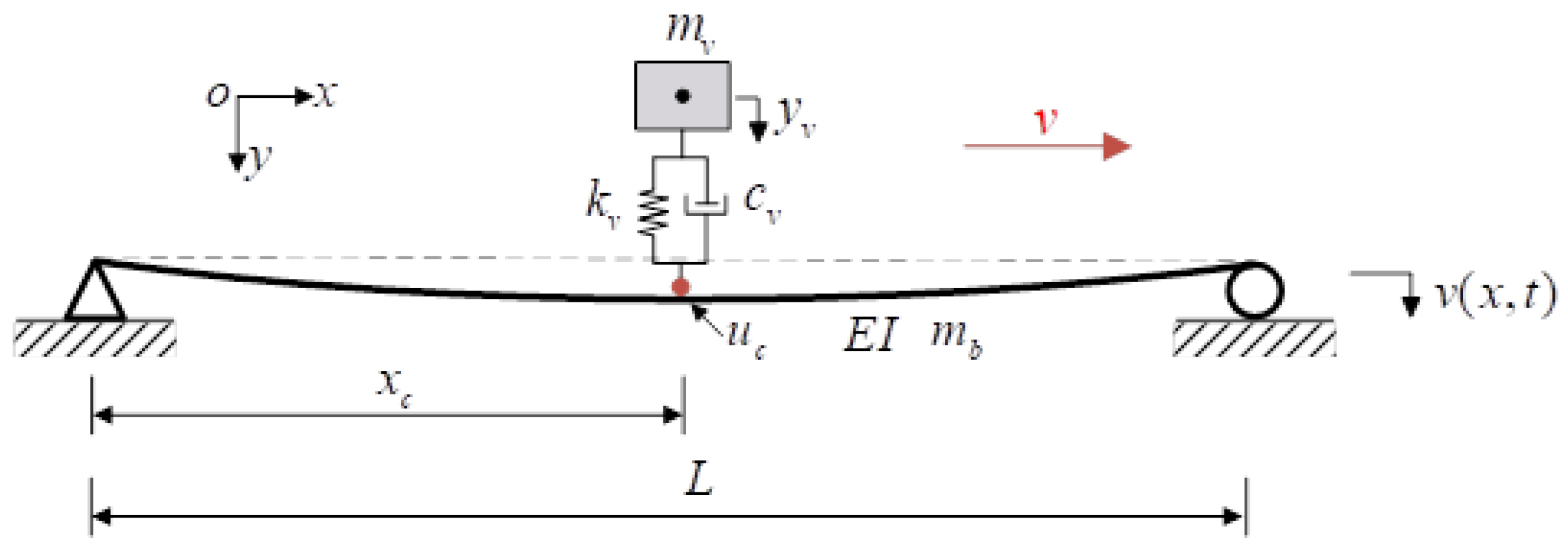
2. Theoretical Background of the Problem

The vehicle model is simplified to a single DOF moving mass with a support spring to better clarify the moving load force identification method proposed in this study. The bridge is set according to simple support boundary conditions. The mechanical model of the vehicle moving over the bridge is shown in Figure 1. The vehicle runs at a constant speed of $v$. As depicted in Figure 1, $EI$ represents bridge bending stiffness, $m_b$ represents unit length weight, L represents bridge span, $v\left(x,t\right)$ represents bridge vertical displacement, and $u_c$ represents contact displacement at the current time step; for the vehicle model, $m_v$ represents vehicle mass, $c_v$ represents the vehicle damping coefficient, and $k_v$ represents the vehicle stiffness coefficient.

Based on Dalembert’s principle, the vehicle dynamics equation can be expressed as:

$$m_v{\ddot{y}}_v\left(t\right)+c_v{\dot{y}}_v(t)+k_v{y}_v(t)=P(t)$$

(1)

where $P\left(t\right)$ is the contact force between the vehicle and bridge; and ${\ddot{y}}_v$(t), ${\dot{y}}_v\left(t\right)$, and $y_v$(t) are the acceleration, velocity, and displacement of the vehicle, respectively.

Based on the Newmark algorithm, the interrelationship between the dynamic responses of moment $t_i$ and moment $t_{i+1}$ can be established as:

$${\dot{y}}_v^{i+1}={\dot{y}}_v^i+\left(1-\gamma \right)\Delta t{\ddot{y}}_v^i+\gamma \Delta t{\ddot{y}}_v^{i+1}$$

(2)

$$y_v^{i+1}=y_v^i+\Delta t{\dot{y}}_v^i+\left(\frac{1}{2}-\beta \right)\Delta t^2{\ddot{y}}_v^i+\beta \Delta t^2{\ddot{y}}_v^{i+1}$$

(3)

where $\gamma =0.5$, $\beta =0.25$; and the superscript “i” and “i + 1” denote the vehicle response at the $t_i$ and $t_{i+1}$ moments, respectively. For simplicity, the same, simplified notations will be adopted in the following equations.

By rewriting Equation (3), the acceleration at the $t_{i+1}$ moment can be obtained as:

$${\ddot{y}}_v^{i+1}=\frac{1}{\beta \Delta t^2}\left(y_v^{i+1}-y_v^i\right)-\frac{1}{\beta \Delta t}{\dot{y}}_v^i-\left(\frac{1}{2\beta }-1\right){\ddot{y}}_v^i$$

(4)

Substituting Equation (4) into Equation (2) yields the velocity response at the $t_{i+1}$ moment, illustrated as:

$${\dot{y}}_v^{i+1}=\frac{\gamma }{\beta \Delta t}\left(y_v^{i+1}-y_v^i\right)+\left(1-\frac{\gamma }{\beta }\right){\dot{y}}_v^i+\left(1-\frac{\gamma }{2\beta }\right)\Delta t{\ddot{y}}_v^i$$

(5)

At the $t_{i+1}$ moment, the vehicle’s motion equation can be expressed as:

$$m_v{\ddot{y}}_v^{i+1}+c_v{\dot{y}}_v^{i+1}+k_v{y}_v^{i+1}=P(t_{i+1})$$

(6)

Subsequently, by substituting Equations (4) and (5) into Equation (6) and merging the similar items, Equation (6) can be simplified as:

$$\widehat{K}{y}_v^{i+1}={\widehat{P}}_{i+1}$$

(7)

where $\widehat{K}$ and ${\widehat{P}}_{i+1}$ represent the equivalent stiffness and external load, respectively, as illustrated:

$$\widehat{K}=k_v+\frac{1}{\beta \Delta t^2}{m}_v+\frac{\gamma }{\beta \Delta t}{c}_v$$

(8)

$$\begin{array}{l}{\widehat{P}}_{i+1}=P(t_{i+1})+\left[\frac{1}{\beta \Delta t^2}{m}_v+\frac{\gamma }{\beta \Delta t}{c}_v\right]y_v^i+\left[\frac{1}{\beta \Delta t}{m}_v+\left(\frac{\gamma }{\beta }-1\right)c_v\right]{\dot{y}}_v^i\\ +\left[\left(\frac{1}{2\beta }-1\right)m_v+\frac{\Delta t}{2}\left(\frac{\gamma }{\beta }-1\right)c_v\right]{\ddot{y}}_v^i\end{array}$$

(9)

For Equation (7), the displacement response $y_v^{i+1}$ at the end of the time step can be obtained as:

$$y_v^{i+1}=A_{0}P(t_{i+1})+A_d{y}_v^i+A_v{\dot{y}}_v^i+A_a{\ddot{y}}_v^i$$

(10)

with

$$A_0={\widehat{K}}^{-1},$$

(11a)

$$A_d={\widehat{K}}^{-1}\left[\frac{1}{\beta \Delta t^2}{m}_v+\frac{\gamma }{\beta \Delta t}{c}_v\right],$$

(11b)

$$A_v={\widehat{K}}^{-1}\left[\frac{1}{\beta \Delta t}{m}_v+\left(\frac{\gamma }{\beta }-1\right)c_v\right],$$

(11c)

$$A_a={\widehat{K}}^{-1}\left[\left(\frac{1}{2\beta }-1\right)m_v+\frac{\Delta t}{2}\left(\frac{\gamma }{\beta }-1\right)c_v\right]$$

(11d)

After obtaining the displacement response $y_v^{i+1}$, the velocity response ${\dot{y}}_v^{i+1}$ at this moment can easily be calculated using Equation (5). Additionally, the constant coefficients matrices in Equation (5) are converted into unit ones in terms of $I={\widehat{K}}^{-1}\widehat{K}$. After combining the same terms, Equation (5) can be unified into an expression similar to Equation (10), expressed as:

$${\ddot{y}}_v^{i+1}=B_{0}P(t_{i+1})+B_d{y}_v^i+B_v{\dot{y}}_v^i+B_a{\ddot{y}}_v^i$$

(12)

with

$$B_0=\frac{\gamma }{\beta \Delta t}{\widehat{K}}^{-1},$$

(13a)

$$B_d=-\frac{\gamma }{\beta \Delta t}{\widehat{K}}^{-1}K,$$

(13b)

$$B_v=\frac{\gamma }{\beta \Delta t}{\widehat{K}}^{-1}\left[\left(\frac{\beta \Delta t}{\gamma }-\Delta t\right)k_v+\frac{1}{\gamma \Delta t}{m}_v\right],$$

(13c)

$$B_a=\frac{\gamma }{\beta \Delta t}{\widehat{K}}^{-1}\left[\left(\frac{\beta \Delta t^2}{\gamma }-\frac{\Delta t^2}{2}\right)k_v+\left(\frac{1}{\gamma }-1\right)m_v\right]$$

(13d)

Similarly, the acceleration response ${\ddot{y}}_v^{i+1}$ can be simplified to the following expression by substituting Equation (10) into Equation (4), expressed as:

$${\ddot{y}}_v^{i+1}=C_{0}P(t_{i+1})+C_d{y}_v^i+C_v{\dot{y}}_v^i+C_a{\ddot{y}}_v^i$$

(14)

with

$$C_0=\frac{1}{\beta \Delta t^2}{\widehat{K}}^{-1},$$

(15a)

$$C_d=-\frac{1}{\beta \Delta t^2}{\widehat{K}}^{-1}K,$$

(15b)

$$C_v=-\frac{1}{\beta \Delta t^2}{\widehat{K}}^{-1}\left(c_v+\Delta t{k}_v\right),$$

(15c)

$$C_a=\frac{1}{\beta \Delta t^2}{\widehat{K}}^{-1}\left[\left(\gamma -1\right)\Delta t{c}_v-\beta \Delta t^2\left(\frac{1}{2\beta }-1\right)k_v\right]$$

(15d)

Combing Equations (10), (12) and (14), one yields:

$$\left[\begin{array}{c}{y}_v^{i+1}\\ {\dot{y}}_v^{i+1}\\ {\ddot{y}}_v^{i+1}\end{array}\right]=\left[\begin{array}{c}{A}_0\\ B_0\\ C_0\end{array}\right]P(t_{i+1})+\left[\begin{array}{ccc}{A}_d& A_v& A_a\\ B_d& B_v& B_a\\ C_d& C_v& C_a\end{array}\right]\left[\begin{array}{c}{y}_v^i\\ {\dot{y}}_v^i\\ {\ddot{y}}_v^i\end{array}\right]$$

(16)

Equation (16) clearly indicates that a recursion formula for the vehicle’s response between the $t_i$ and $t_{i+1}$ moments is established. On this basis, the displacement, velocity, and acceleration responses of the vehicle at the $t_i$ moment are written using the above recursion formula as:

$$\left[\begin{array}{c}{y}_v^i\\ {\dot{y}}_v^i\\ {\ddot{y}}_v^i\end{array}\right]={\displaystyle \sum _{j=0}^{i-1}{\left[\begin{array}{ccc}{A}_d& A_v& A_a\\ B_d& B_v& B_a\\ C_d& C_v& C_a\end{array}\right]}^j}\left[\begin{array}{c}{A}_0\\ B_0\\ C_0\end{array}\right]P_i+{\left[\begin{array}{ccc}{A}_d& A_v& A_a\\ B_d& B_v& B_a\\ C_d& C_v& C_a\end{array}\right]}^i\left[\begin{array}{c}{y}_v^0\\ {\dot{y}}_v^0\\ {\ddot{y}}_v^0\end{array}\right]$$

(17)

where $y_v^0$, ${\dot{y}}_v^0$, and ${\ddot{y}}_v^0$ are the initial displacement, velocity, and acceleration responses, respectively.

In the context of this study, the acceleration transducers are installed on the test vehicle. The vehicle’s acceleration response is recorded first, followed by the application of the proposed algorithm to retrieve the moving loads through the recorded data. Supposing the output response of the test vehicle is represented by vector $\mathbf{y}\left(t\right)\in {\mathbf{R}}^{m\times 1}$, and $m$ is the number of measured responses,

$$Y=R_a{\ddot{y}}_v^{}+R_v{\dot{y}}_v^{}+R_{d}y=\left[\begin{array}{ccc}{R}_d& & \\ & R_v& \\ & & R_a\end{array}\right]\left[\begin{array}{c}{y}_v\\ {\dot{y}}_v^{}\\ {\ddot{y}}_v^{}\end{array}\right]=R\left[\begin{array}{c}{y}_v\\ {\dot{y}}_v^{}\\ {\ddot{y}}_v^{}\end{array}\right]$$

(18)

where $\mathbf{R}=diag\left[\begin{array}{ccc}{R}_d& R_v& R_a\end{array}\right]$. Given the installation of a single acceleration transducer on the test vehicle, $R_a=1$, $R_d=R_v=0$.

Substituting Equation (17) into Equation (18), one yields the following equation:

$$Y\left(t_i\right)={\displaystyle \sum _{j=0}^{i-1}\mathbf{R}{\left[\begin{array}{ccc}{A}_d& A_v& A_a\\ B_d& B_v& B_a\\ C_d& C_v& C_a\end{array}\right]}^j}\left[\begin{array}{c}{A}_0\\ B_0\\ C_0\end{array}\right]P_i+\mathbf{R}{\left[\begin{array}{ccc}{A}_d& A_v& A_a\\ B_d& B_v& B_a\\ C_d& C_v& C_a\end{array}\right]}^i\left[\begin{array}{c}{y}_v^0\\ {\dot{y}}_v^0\\ {\ddot{y}}_v^0\end{array}\right]$$

(19)

Assuming the null initial conditions, i.e., $y_v^0={\dot{y}}_v^0={\ddot{y}}_v^0=0$, a new matrix ${\mathbf{H}}_k$ is defined as:

$${\mathbf{H}}_k=\mathbf{R}{\left[\begin{array}{ccc}{A}_d& A_v& A_a\\ B_d& B_v& B_a\\ C_d& C_v& C_a\end{array}\right]}^k\left[\begin{array}{c}{A}_0\\ B_0\\ C_0\end{array}\right]$$

(20)

Using the matrix ${\mathbf{H}}_k$, Equation (19) can be written in matrix convolution form within the time interval [$t_1$ $t_n$], expressed as:

$$\mathbf{Y}={\mathbf{H}}_L\mathbf{P}$$

(21)

where

$$\mathbf{Y}=\left\{\begin{array}{c}\mathbf{y}\left(t_1\right)\\ \mathbf{y}\left(t_2\right)\\ \dots \\ \mathbf{y}\left(t_n\right)\end{array}\right\},$$

(22a)

$${\mathbf{H}}_L=\left[\begin{array}{cccc}{\mathbf{H}}_0& 0& \dots & 0\\ {\mathbf{H}}_1& {\mathbf{H}}_0& \dots & 0\\ \dots & \dots & \dots & \dots \\ {\mathbf{H}}_{n-1}& {\mathbf{H}}_{n-2}& \dots & {\mathbf{H}}_0\end{array}\right],$$

(22b)

$$\mathbf{P}=\left\{\begin{array}{c}\mathbf{P}\left(t_1\right)\\ \mathbf{P}\left(t_2\right)\\ \dots \\ \mathbf{P}\left(t_n\right)\end{array}\right\}$$

(22c)

Equation (21) can be directly solved to acquire the load vector $\mathbf{P}$ as:

$$\mathbf{P}={\left({\mathbf{H}}_L^T{\mathbf{H}}_L\right)}^{-1}{\mathbf{H}}_L^T\mathbf{Y}$$

(23)

Given that the linear correlation between the columns of matrix ${\mathbf{H}}_L$ is large, the determinant of ${\mathbf{H}}_L^T{\mathbf{H}}_L$ is close to zero, implying that the direct solution for Equation (23) becomes an unsettled problem. In other words, the load vector cannot be calculated using Equation (23). To overcome this obstacle, the Tikhonov regularisation approach is utilised in the subsequent section.

3. Tikhonov Regularisation

In practice, the equation used for identifying a moving load often manifests ill-posedness due to the coefficient matrix. The ill-posedness problem is exhibited as a loss of rank and the presence of pathology; thus, the paramount task lies in solving these issues for the force identification. When data collected at a high sampling frequency from measurement points exceed the number of moving loads, the problem of rank loss no longer exists. Consequently, the critical aspect for identifying the moving load centres on solving the pathological problem. To this end, this study employs Tikhonov regularisation to solve the instability encountered during the process of moving load identification.

As depicted in Equation (23), the solution for identifying the moving load is $\mathbf{P}={\left({\mathbf{H}}_L^T{\mathbf{H}}_L\right)}^{-1}{\mathbf{H}}_L^T\mathbf{Y}$. Nevertheless, the inversion process for ${\mathbf{H}}_L^T{\mathbf{H}}_L$ could become unstable due to the significant impacts of the numerous coefficient conditions and external noise in the measured data. As a result of such instabilities, the solution of the load vector $\mathbf{P}$ deviates greatly from the actual vehicle axle load. In addressing the pathological problem, the Tikhonov regularisation method applies a weak smoothness constraint and selects the approximate solutions of the equation. The actual process for Tikhonov regularisation thus involves solving the minimum value of the following equation:

$$min=\left\{{\Vert {\mathbf{H}}_L\mathbf{P}-\mathbf{Y}\Vert }_2+{\lambda }^2{\Vert \mathbf{P}\Vert }_2\right\} (\lambda \ge 0)$$

(24)

where ${\Vert ·\Vert }_2$ signifies the two-dimensional norm of the vector, and $\lambda$ signifies a regularisation parameter. From Equation (24), it can be observed that the Tikhonov regularisation method actually serves to find the minimum of the residual two-dimensional norm ${\Vert {\mathbf{H}}_L\mathbf{P}-\mathbf{Y}\Vert }_2$ and the two-dimensional norm of the solution.

The L-curve principle is employed to obtain the optimal solution and to identify the optimal regular parameter $\lambda$. As a raph-based parameter selection method, the L-curve principle involves plotting two quantities, the solution norm $\log {\Vert {\mathbf{P}}_{\lambda }\Vert }_2$ (y axis) and the residual norm $\log {\Vert {\mathbf{H}}_L{\mathbf{P}}_{\lambda }-\mathbf{Y}\Vert }_2$ (x axis), on the logarithmic coordinate scale to find the equilibrium point, illustrated in Figure 2. At the corner point of the L-curve, both the solution norm and the residual norm are maintained in a balanced dynamic equilibrium, indicating that the point represents the optimal regularisation parameter value.

4. Finite Element Method for Vehicle–Bridge Interaction Analysis

A vehicle–bridge interaction (VBI) element with road surface roughness r was used, illustrated in Figure 3. The test vehicle is modelled as a sprung mass $m_v$ supported by a spring of stiffness $k_v$ and a dashpot of damping coefficient $c_v$. The coordinate $x_c$ represents the position of the contact point in the element local coordinate. The equation of motion for the VBI element can be expressed as:

$$\begin{array}{l}\left[\begin{array}{cc}{m}_v& 0\\ 0& \left[m_b\right]\end{array}\right]\left\{\begin{array}{c}{\ddot{y}}_v\\ \left\{{\ddot{u}}_b\right\}\end{array}\right\}+\left[\begin{array}{cc}{c}_v& -c_v{\left\{N\right\}}_c^T\\ -c_v{\left\{N\right\}}_c& \left[c_b\right]+c_v{\left\{N\right\}}_c{\left\{N\right\}}_c^T\end{array}\right]\left\{\begin{array}{c}{\dot{y}}_v\\ \left\{{\dot{u}}_b\right\}\end{array}\right\}\\ +\left[\begin{array}{cc}{k}_v& -k_v{\left\{N\right\}}_c^T-v{c}_v{\left\{N^{\prime }\right\}}_c^T\\ -k_v{\left\{N\right\}}_c& \left[k_b\right]+v{c}_v{\left\{N\right\}}_c{\left\{N^{\prime }\right\}}_c^T+k_v{\left\{N\right\}}_c{\left\{N\right\}}_c^T\end{array}\right]\left\{\begin{array}{c}{y}_v\\ \left\{u_b\right\}\end{array}\right\}=\left\{\begin{array}{c}{c}_{v}v{r}_c^{\prime }+k_v{r}_c\\ -\left(c_{v}v{r}_c^{\prime }+k_v{r}_c+m_{v}g\right){\left\{N\right\}}_c\end{array}\right\}\end{array}$$

(25)

where $y_v$ and $\left\{u_b\right\}$ represent the displacement of the vehicle and that of the bridge element, respectively, and a dot represents the derivative with respect to time t; $\left[m_b\right]$, $\left[c_b\right]$, and $\left[k_b\right]$ denote the mass, damping, and stiffness matrices of the bridge element, respectively; $r_c$ represents the road surface roughness at the contact point $x_c$; and ${\left\{N\right\}}_c$ represents the cubic Hermitian function evaluated at the contact point $x_c$, whose detailed expression is based on the literature.

The global equation of motion for the entire bridge system is formulated by assembling all the bridge elements (with and without the vehicle) and imposing the boundary conditions, i.e., zero vertical displacement and moments, at the two ends. Subsequently, the Newmark-$\beta$ method, with $\beta$ = 0.25 and $\gamma$ = 0.5, is adopted for the response to the coupled dynamic equation.

5. Identifying Procedures for the Proposed Method

The proposed identification method primarily includes the following three steps:

Step 1: The motion equation of the vehicle–bridge coupling system under a moving test vehicle is established. The vehicle’s displacement, velocity, and acceleration responses are obtained via numerical calculation.

Step 2: $A_i$, $B_i$, and $C_i$ (i = 0, d, v, and a) are calculated based on the properties of the test vehicle. According to the sensor type and its layout position on the vehicle, the matrix is determined, and the vector $\mathbf{Y}$ and matrix ${\mathbf{H}}_k$ are calculated using the vehicle response obtained in Step 1.

Step 3: Substituting the vector $\mathbf{Y}$ and matrix ${\mathbf{H}}_k$ obtained in Step 2 into Equation (23) and using the Tikhonov regularisation method to solve the ill-conditioned problem, the moving force as the test vehicle traverses on the bridge can finally be identified.

6. Numerical Verifications

In order to authenticate the reliability of the proposed method, a numerical verification is conducted within this section. This is achieved by employing the identification procedure delineated in Section 5. The contact response, obtained through numerical calculation, is taken as the real value, whereas the contact response identified in reverse is taken as the predicted one. The accuracy of the proposed method is verified by comparing these two values. The properties of the vehicle and bridge are listed in

Table 1. Properties of the vehicle and bridge.

Vehicle
Mass	$m_v$	kg	1200
Spring stiffness	$k_v$	N/m	5.0 × 104
Bridge
Young’s modulus	$E$	N/m2	2.75 × 1010
Moment of inertia	$I$	m4	0.20
Mass per unit length	$m$	kg/m	2400
Length	$L$	m	30

. The vehicle traverses the bridge at a constant speed of 10 m/s. A random road roughness sample with Grade A is generated based on the ISO 8606 specification, with the simulated road roughness sample illustrated in Figure 4. It is assumed that the vehicle maintains a zero initial state, with a step size of 0.001 s adopted for the numerical calculation. Employing the vehicle and bridge parameters as listed in Table 1, the vehicle acceleration response is demonstrated in Figure 5.

To evaluate the predicted accuracy of the proposed method, the root mean square error (RMSE) between the predicted value and the real one is used herein, calculated as:

$$\mathrm{RMSE}\left(y,\widehat{y}\right)=\sqrt{\frac{1}{n}{\displaystyle \sum _{i=1}^n{\left(y_i-{\widehat{y}}_i\right)}^2}}$$

(26)

where $y_i$ and ${\widehat{y}}_i$ denote the predicted and real contact forces at time step i, respectively, and n stands for the total number of time steps. As derived from the definition of the RMSE, the value is smaller, while the predicted accuracy is higher for the proposed method.

Figure 6 presents a comparison of the moving load identification results between the real and predicted values. It can be observed from the figure that the results for the predicated moving load align well with the real ones, despite the influence of road roughness. The RMSE value is 0.1379, being close to null for the case considered, implying that the proposed method has a high accuracy in identifying the moving contact force. Given the aforementioned comparison results, the reliability of the proposed method is verified.

Furthermore, the conventional time domain method (CTM) is utilised to further validate the feasibility of the proposed method. Differing from the method presented here, the CTM involves installing sensors on the bridge to record the bridge acceleration responses as the vehicle passes over it. Two different sensor deployments are considered for the CTM, referred to as Case 1 and Case 2. The specific deployments for both cases are listed in

Table 2. Simulation cases for the conventional time domain (CTM) method.

No. Case	Locations for the Sensors	Quantity Sensors
Case 1	1/4 span, 1/2 span, and 3/4 span	Three
Case 2	1/6 span, 1/3 span, 1/2 span, 2/3 span, and 5/6 span	Five

.

Figure 7 depicts the comparison results of the moving contact force for various identified methods. It can be observed that the contact force identified using the proposed method coincides closely with Case 2 using the CTM and the real values, whereas a distinct disparity is observed with the prediction result of Case 1. In comparison with the CTM, the proposed method utilises fewer sensors to obtain the moving contact force with high precision. However, a greater number of sensors must be adopted to ensure the identification accuracy of the CTM. Consequently, the comparison results further validate the accuracy and advantages of the proposed method.

7. Parametric Analyses of Various Influencing Factors

The accuracy of the proposed method was verified in the preceding section. This section further studies the robustness of the method, performing a sensitivity analysis of various external factors, i.e., road roughness, running speed, and noise level, that may affect the recognition accuracy.

7.1. Effect of Road Roughness

Using the simulation method outlined in the ISO 8606 specification, random road roughness samples for Grades B and C were generated, as illustrated in Figure 8. It becomes evident that pavement classes B and C possess greater amplitudes and higher frequencies in comparison to Class A. Figure 9 showcases a comparison of the moving force identification results at various pavement roughness levels. It can be observed that the vehicle–bridge contact force gradually rises with the increasing road surface grade. Notwithstanding the heightened roughness of classes B and C, the moving load identification employing the proposed method remains consistent with the real one. The RMSE values for Grades B and C stand at 0.1380 and 0.1384, respectively. Comparatively, the identified accuracy for these cases is slightly reduced compared to the result for Grade A, as depicted in Section 6, yet continues to present high precision. Consequently, the proposed method exhibits minimal susceptibility to road roughness in identifying the moving load. Furthermore, higher pavement grades lead to a more significant acceleration response, favouring the identification of the moving contact force.

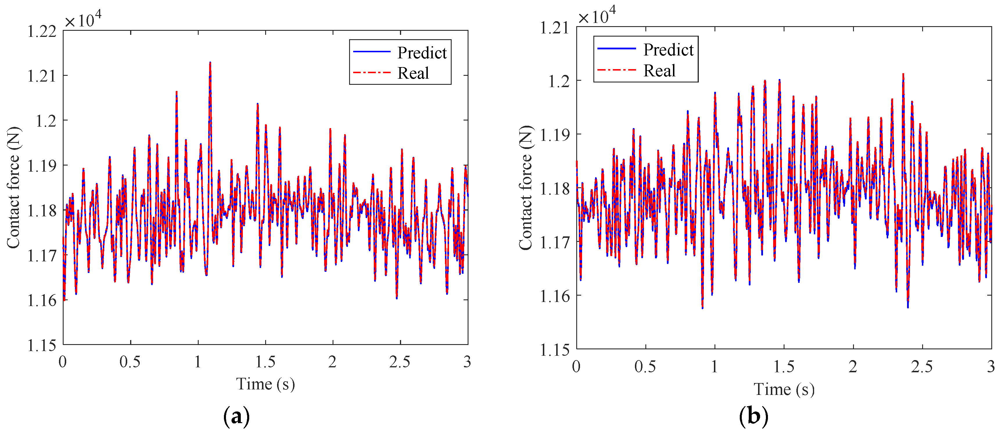
7.2. Effect of Running Speed

The efficiency of identification using the proposed method is directly determined by the vehicle running speed in real-world projects. Therefore, this section considers two speeds, namely, v = 5 and 15 m/s. The pavement grade adheres to Class C, and the other parameters align with those used in Section 3. Figure 10 compares the contact force identification results at different vehicle operating speeds. It can be observed that the contact force rises with the increasing vehicle speed. The moving force remains well identified at different vehicle running speeds using the proposed method, implying that the running speed of the vehicle exerts little effect on it. From the perspective of identification accuracy, the RMSE values for the running speeds of 5 and 15 m/s are 0.0687 and 0.2087, respectively. The results indicate that the identified precision may undergo limited reductions, while the proposed method can maintain a high precision even at a rapid running speed. To ensure the test precision and efficiency, however, an intermediate speed is recommended for field applications employing the proposed method. The primary reason for this lies in the fact that a smaller volume of data, obtained at the same sampling frequency for a limited length of the bridge, will result in an inferior identification accuracy. Thus, for the case under consideration, a test speed of 10 m/s will be optimal.

7.3. Effect of the Environmental Noise Level

In practice, measured data inevitably incur contamination from environmental noise. To investigate the feasibility of the proposed method, four environmental noise levels of 2%, 5%, 10%, and 20% are applied to the measured data. The expression is defined as:

$${\ddot{y}}_{vp}={\ddot{y}}_v+E_p{N}_s{\sigma }_{{\ddot{y}}_v}$$

(27)

where ${\ddot{y}}_v$ denotes the original vehicle acceleration response. $E_p$ denotes the noise level. $N_s$ and ${\sigma }_{{\ddot{y}}_v}$ represent the mean and standard deviation of the vehicle’s acceleration response.

Figure 11 demonstrates a comparison of the moving force identification results at varying environmental noise levels. The RMSE values for $E_p$ = 2%, 5%, 10%, and 20% stand at 3.1940, 4.9653, 14.5237, and 36.3568, respectively. It can be seen that the recognition results are worse than those without noise, but the recognition accuracy is generally maintained at a higher level. Even at a 20% environmental noise level, the recognition results remain highly accurate. Therefore, the proposed method for identifying moving contact force presents a certain robustness to environmental noise. However, it is suggested that the environmental noise level should be controlled within 10% to ensure test precision when applying the proposed method in field tests.

8. Conclusions

In this study, we introduced a novel method for moving load identification on bridges, using a vehicle–bridge coupled vibration theory and the Newmark-$\beta$ algorithm. This approach requires sensor arrangement solely on the vehicle, recording its responses as it traverses the bridge. Based on the obtained responses, the moving force can be swiftly identified via the proposed method. Tikhonov regularisation is employed to overcome the ill-conditioned nature of the inverse problem so as to enhance the recognition accuracy. A single DoF vehicle traversing a simply supported beam is used as an example to numerically verify the proposed method’s reliability by comparing the predicted values with the real ones. Additionally, we examined several typical external factors to discuss the robustness of the proposed method. Based on the theoretical derivations and the data adopted in our analysis, the following conclusions were drawn:

(1)

Unlike the existing identification methods, our approach does not necessitate the installation of sensors on the bridge. Instead, the moving contact force can be identified readily through sensors installed on the moving vehicle. This provides a new idea for moving load identification on small- and medium-span bridges.

(2)

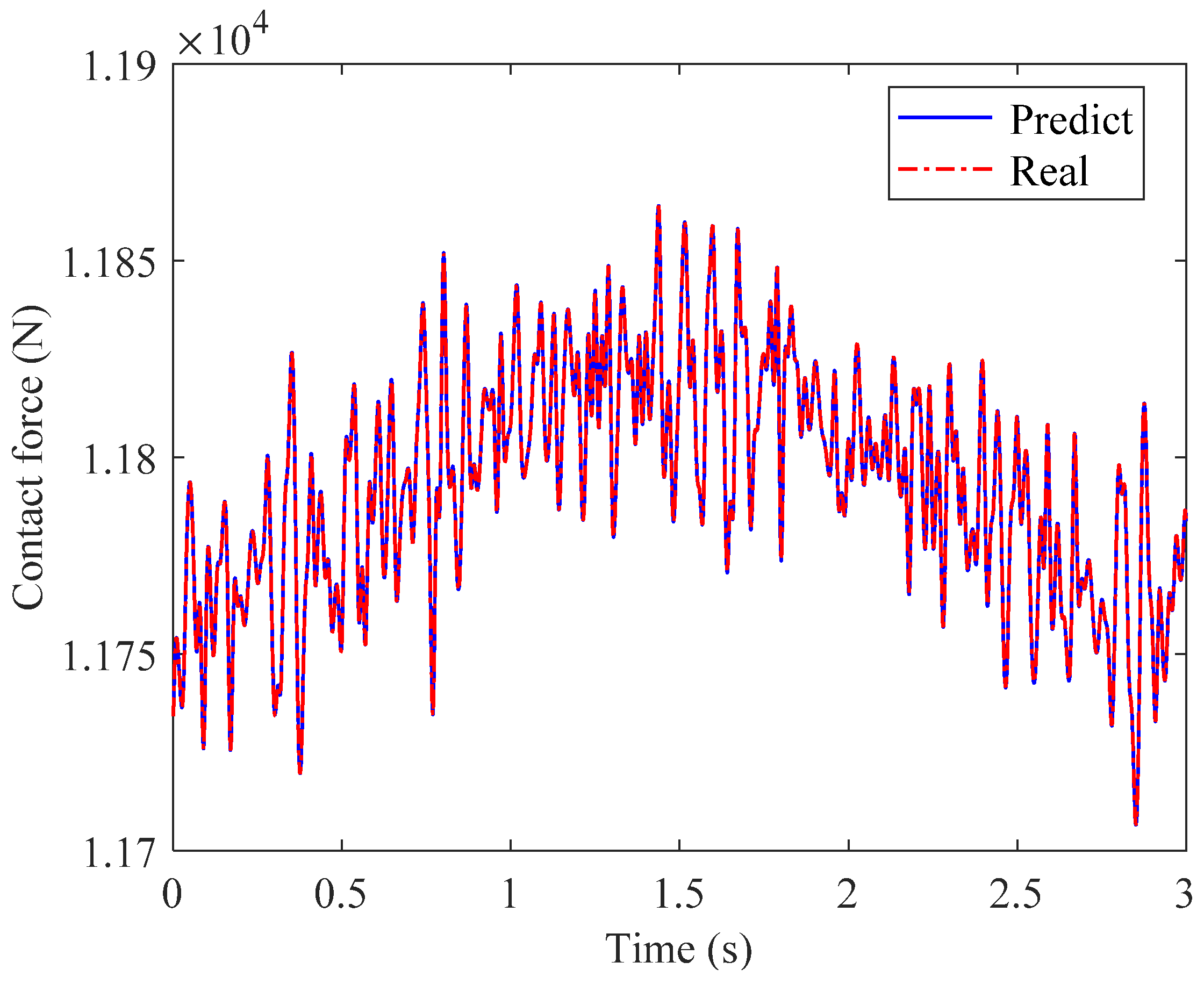
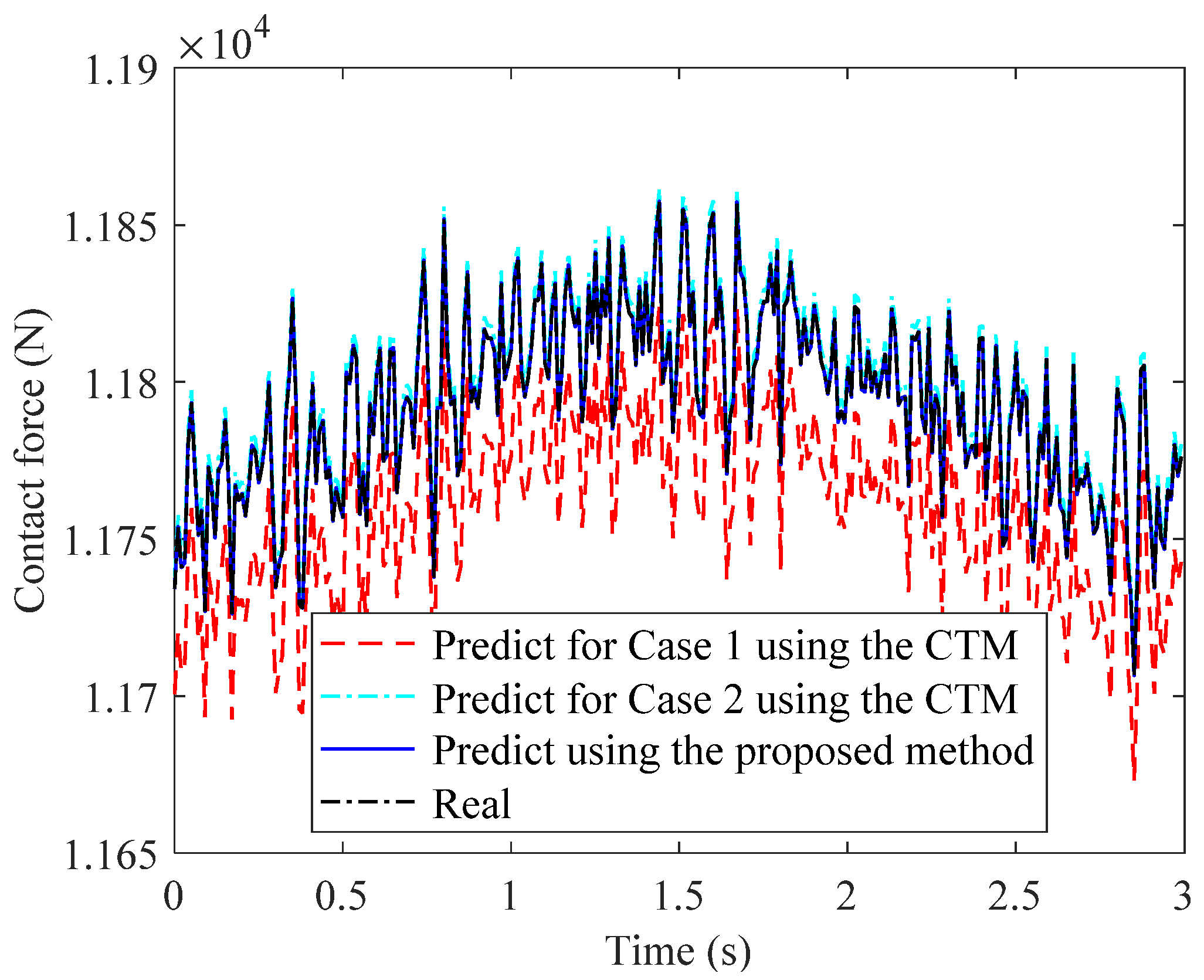
The proposed method demonstrates high precision in identifying the moving contact force by comparing with the real values and those identified using the CTM method.

(3)

The moving load can be effectively identified even under conditions of poor road roughness in Class C.

(4)

The effect of moving speed is limited for the proposed method; however, an intermediate speed of 10 m/s is recommended for field testing.

(5)

Environmental noise can affect the identification accuracy to an acceptable extent. Control of the environment noise level within 10% for the proposed method is recommended in actual applications.

Though the proposed method is based on a single-DOF vehicle model moving over a simply supported bridge, it is adaptable to multi-DOF vehicle models and other bridge types, i.e., elastic, clamped, fixed, and general support boundary conditions. Consequently, our future studies will focus on identifying the moving force using multi-DOF vehicle models and conduct further experimental validations of the proposed method’ accuracy.

References

1. He, X.H.; Shi, K.; Wu, T. An integrated structural health monitoring system for the Xijiang high-speed railway arch bridge. Smart Struct. Syst. 2018, 21, 611–621. [Google Scholar]
2. He, Z.; Li, W.; Salehi, H.; Zhang, H.; Zhou, H.; Jiao, P. Integrated structural health monitoring in bridge engineering. Autom. Constr. 2022, 136, 104168. [Google Scholar] [CrossRef]
3. Tian, Y.; Chen, C.; Sagoe-Crentsil, K.; Zhang, J.; Duan, W. Intelligent robotic systems for structural health monitoring: Applications and future trends. Autom. Constr. 2022, 139, 104273. [Google Scholar] [CrossRef]
4. Niu, J.; Li, Z.; Zhuo, Y.; Di, H.; Wei, J.; Wang, X.; Guo, Y.; Li, S. Robust correlation mapping of train-induced stresses for high-speed railway bridge using convolutional denoising autoencoder. Struct. Health Monit. 2023, 22, 832–845. [Google Scholar] [CrossRef]
5. Lei, X.; Xia, Y.; Wang, A.; Jian, X.; Zhong, H.; Sun, L. Mutual information based anomaly detection of monitoring data with attention mechanism and residual learning. Mech. Syst. Signal Process. 2023, 182, 109607. [Google Scholar] [CrossRef]
6. Tang, Z.; Chen, Z.; Bao, Y.; Li, H. Convolutional neural network-based data anomaly detection method using multiple information for structural health monitoring. Struct. Control Health Monit. 2019, 26, e2296. [Google Scholar] [CrossRef] [Green Version]
7. Ouyang, H. Moving-load dynamic problems: A tutorial (with a brief overview). Mech. Syst. Signal Process. 2011, 25, 2039–2060. [Google Scholar] [CrossRef]
8. Zhu, X.Q.; Law, S.S. Recent developments in inverse problems of vehicle–bridge interaction dynamics. J. Civ. Struct. Health Monit. 2016, 6, 107–128. [Google Scholar] [CrossRef]
9. Liu, R.; Dobriban, E.; Hou, Z.; Qian, K. Dynamic load identification for mechanical systems: A review. Arch. Comput. Methods Eng. 2022, 29, 831–863. [Google Scholar] [CrossRef]
10. Yu, Y.; Cai, C.S.; Deng, L. State-of-the-art review on bridge weigh-in-motion technology. Adv. Struct. Eng. 2016, 19, 1514–1530. [Google Scholar] [CrossRef]
11. Paul, D.; Roy, K. Application of bridge weigh-in-motion system in bridge health monitoring: A state-of-the-art review. Struct. Health Monit. 2023, 14759217231154431. [Google Scholar] [CrossRef]
12. Law, S.S.; Chan, T.H.; Zeng, Q.H. Moving force identification: A time domain method. J. Sound Vib. 1997, 201, 1–22. [Google Scholar] [CrossRef]
13. Zhu, X.Q.; Law, S.S. Moving forces identification on a multi-span continuous bridge. J. Sound Vib. 1999, 228, 377–396. [Google Scholar] [CrossRef]
14. Liu, J.; Meng, X.; Jiang, C.; Han, X.; Zhang, D. Time-domain Galerkin method for dynamic load identification. Int. J. Numer. Methods Eng. 2016, 105, 620–640. [Google Scholar] [CrossRef]
15. Liu, J.; Meng, X.; Zhang, D.; Jiang, C.; Han, X. An efficient method to reduce ill-posedness for structural dynamic load identification. Mech. Syst. Signal Process. 2017, 95, 273–285. [Google Scholar] [CrossRef]
16. Chen, Z.; Qin, L.; Chan, T.H.; Yu, L. A novel preconditioned range restricted GMRES algorithm for moving force identification and its experimental validation. Mech. Syst. Signal Process. 2021, 155, 107635. [Google Scholar] [CrossRef]
17. Yu, L.; Chan, T.H. Moving force identification based on the frequency–time domain method. J. Sound Vib. 2003, 261, 329–349. [Google Scholar] [CrossRef]
18. Lage, Y.E.; Maia, N.M.M.; Neves, M.M.; Ribeiro, A.M.R. Force identification using the concept of displacement transmissibility. J. Sound Vib. 2013, 332, 1674–1686. [Google Scholar] [CrossRef]
19. Aucejo, M.; De Smet, O. A space-frequency multiplicative regularization for force reconstruction problems. Mech. Syst. Signal Process. 2018, 104, 1–18. [Google Scholar] [CrossRef] [Green Version]
20. He, Z.C.; Lin, X.Y.; Li, E. A novel method for load bounds identification for uncertain structures in frequency domain. Int. J. Comput. Methods 2018, 15, 1850051. [Google Scholar] [CrossRef]
21. Yan, W.J.; Yuen, K.V. A new probabilistic frequency-domain approach for influence line extraction from static transmissibility measurements under unknown moving loads. Eng. Struct. 2020, 216, 110625. [Google Scholar] [CrossRef]
22. Sanchez, J.; Benaroya, H. Review of force reconstruction techniques. J. Sound Vib. 2014, 333, 2999–3018. [Google Scholar] [CrossRef]
23. Tran, H.; Inoue, H. Development of wavelet deconvolution technique for impact force reconstruction: Application to reconstruction of impact force acting on a load-cell. Int. J. Impact Eng. 2018, 122, 137–147. [Google Scholar] [CrossRef]
24. Chen, Z.; Chan, T.H. A truncated generalized singular value decomposition algorithm for moving force identification with ill-posed problems. J. Sound Vib. 2017, 401, 297–310. [Google Scholar] [CrossRef]
25. Chen, Z.; Chan, T.H.; Nguyen, A. Moving force identification based on modified preconditioned conjugate gradient method. J. Sound Vib. 2018, 423, 100–117. [Google Scholar] [CrossRef]
26. Chen, Z.; Chan, T.H.; Nguyen, A.; Yu, L. Identification of vehicle axle loads from bridge responses using preconditioned least square QR-factorization algorithm. Mech. Syst. Signal Process. 2019, 128, 479–496. [Google Scholar] [CrossRef] [Green Version]
27. Chen, Z.; Qin, L.; Zhao, S.; Chan, T.H.; Nguyen, A. Toward efficacy of piecewise polynomial truncated singular value decomposition algorithm in moving force identification. Adv. Struct. Eng. 2019, 22, 2687–2698. [Google Scholar] [CrossRef]
28. Chen, Z.; Chan, T.H.; Yu, L. Comparison of regularization methods for moving force identification with ill-posed problems. J. Sound Vib. 2020, 478, 115349. [Google Scholar] [CrossRef]
29. Chen, Z.; Deng, L.; Kong, X. Modified truncated singular value decomposition method for moving force identification. Adv. Struct. Eng. 2022, 25, 2609–2623. [Google Scholar] [CrossRef]
30. Pan, C.D.; Yu, L.; Liu, H.L.; Chen, Z.P.; Luo, W.F. Moving force identification based on redundant concatenated dictionary and weighted l1-norm regularization. Mech. Syst. Signal Process. 2018, 98, 32–49. [Google Scholar] [CrossRef]
31. Pan, C.; Ye, X.; Zhou, J.; Sun, Z. Matrix regularization-based method for large-scale inverse problem of force identification. Mech. Syst. Signal Process. 2020, 140, 106698. [Google Scholar] [CrossRef]
32. Pan, C.; Huang, Z.; You, J.; Li, Y.; Yang, L. Moving force identification based on sparse regularization combined with moving average constraint. J. Sound Vib. 2021, 515, 116496. [Google Scholar] [CrossRef]
33. Chudong, P.; Liwen, Z.; Xijun, Y.; Zhuo, S. Vehicle weight identification based on equivalent loads reconstructed from responses of beam-like bridge. J. Sound Vib. 2022, 534, 117072. [Google Scholar] [CrossRef]
34. Zhou, H.C.; Li, H.N.; Yang, D.H.; Yi, T.H. Moving force identification of simply supported bridges through the integral time domain method. J. Sound Vib. 2022, 534, 117046. [Google Scholar] [CrossRef]
35. Zhang, Z.H.; He, W.Y.; Ren, W.X. Moving force identification based on learning dictionary with double sparsity. Mech. Syst. Signal Process. 2022, 170, 108811. [Google Scholar] [CrossRef]
36. He, W.Y.; Li, Y.L.; Yi, J.X.; Ren, W.X. Time-domain identification of moving load on beam type bridges considering interval uncertainty in finite element model. Mech. Syst. Signal Process. 2023, 191, 110168. [Google Scholar] [CrossRef]
37. Newmark, N.M. A method of computation for structural dynamics. J. Eng. Mech. Div. 1959, 85, 67–94. [Google Scholar] [CrossRef]
38. Liu, K.; Law, S.S.; Zhu, X.Q.; Xia, Y. Explicit form of an implicit method for inverse force identification. J. Sound Vib. 2014, 333, 730–744. [Google Scholar] [CrossRef]
39. Jiang, J.; Seaid, M.; Mohamed, M.S.; Li, H. Inverse algorithm for real-time road roughness estimation for autonomous vehicles. Arch. Appl. Mech. 2020, 90, 1333–1348. [Google Scholar] [CrossRef]
40. Jiang, J.; Ding, M.; Li, J. A novel time-domain dynamic load identification numerical algorithm for continuous systems. Mech. Syst. Signal Process. 2021, 160, 107881. [Google Scholar] [CrossRef]
41. Pourzeynali, S.; Zhu, X.; Ghari Zadeh, A.; Rashidi, M.; Samali, B. Comprehensive study of moving load identification on bridge structures using the explicit form of Newmark-β method: Numerical and experimental studies. Remote Sens. 2021, 13, 2291. [Google Scholar] [CrossRef]
42. Xin, J.; Jiang, Y.; Zhou, J.; Peng, L.; Liu, S.; Tang, Q. Bridge deformation prediction based on SHM data using improved VMD and conditional KDE. Eng. Struct. 2022, 261, 114285. [Google Scholar] [CrossRef]
43. Jiang, Y.; Hui, Y.; Wang, Y.; Peng, L.; Huang, G.; Liu, S. A novel eigenvalue-based iterative simulation method for multi-dimensional homogeneous non-Gaussian stochastic vector fields. Struct. Saf. 2023, 100, 102290. [Google Scholar] [CrossRef]
44. Li, S.; Xin, J.; Jiang, Y.; Wang, C.; Zhou, J.; Yang, X. Temperature-induced deflection separation based on bridge deflection data using the TVFEMD-PE-KLD method. J. Civ. Struct. Health Monit. 2023, 13, 781–797. [Google Scholar] [CrossRef]
45. Yang, Y.B.; Lin, C.W.; Yau, J.D. Extracting bridge frequencies from the dynamic response of a passing vehicle. J. Sound Vib. 2004, 272, 471–493. [Google Scholar] [CrossRef]
46. Yang, Y.B.; Yang, J.P.; Wu, Y.; Zhang, B. Vehicle Scanning Method for Bridges; John Wiley & Sons: Hoboken, NJ, USA, 2019. [Google Scholar]
47. Yang, Y.B.; Wang, Z.L.; Shi, K.; Xu, H.; Wu, Y.T. State-of-the-art of vehicle-based methods for detecting various properties of highway bridges and railway tracks. Int. J. Struct. Stab. Dyn. 2020, 20, 2041004. [Google Scholar] [CrossRef]
Figure 1. Mechanical model of the vehicle–bridge system.
Buildings 13 01481 g001
Figure 2. L-curve.
Buildings 13 01481 g002
Figure 3. VBI element.
Buildings 13 01481 g003
Figure 4. Random road roughness sample.
Buildings 13 01481 g004
Figure 5. Acceleration response of the test vehicle.
Buildings 13 01481 g005
Figure 6. Comparison results of the contact force for the vehicle–bridge system.
Buildings 13 01481 g006
Figure 7. Comparison results of the contact force for various identified methods.
Buildings 13 01481 g007
Figure 8. Road roughness samples for various class levels.
Buildings 13 01481 g008
Figure 9. Comparison results of contact force for the vehicle–bridge system at various class levels: (a) Class B. (b) Class C.
Buildings 13 01481 g009
Figure 10. Comparison results of the contact force for the vehicle–bridge system at various running speeds: (a) 5 m/s. (b) 15 m/s.
Buildings 13 01481 g010
Figure 11. Comparison results of contact force for the vehicle–bridge system under various environmental noise levels: (a) E p = 2 % . (b) E p = 5 % . (c) E p = 10 % . (d) E p = 20 % .
Buildings 13 01481 g011aBuildings 13 01481 g011b