Comparison of the Stability and Accuracy of Deterministic Project Cost Prediction Methods in Earned Value Management

Abstract

Completing a project on time and on budget are essential factors for the success of any project. One technique that allows predicting the final cost of a project is earned value management (EVM). In this technique, different mathematical methods for predicting the final project cost have been proposed over the last 30 years. These formulas make use of activities’ actual costs and durations as the project progresses. EVM is a technique widely used by many project management professionals. However, very few studies have compared the stability and accuracy of the multiple existing methods for predicting the final cost of the project (commonly abbreviated as estimated cost at completion, EAC). This study compares the stability and accuracy of 30 deterministic cost prediction methods (EAC) in EVM. For this purpose, a representative database of 4100 simulated projects of various topological structures is used. Our results suggest that the methods with the simplest mathematical configurations achieve better stability and accuracy performance. Knowing which EVM methods are the most stable and accurate for predicting the final cost of the project will help project practitioners choose the most reliable cost prediction techniques when they are managing their own projects in real contexts.

1. Introduction

Completing a construction project within the expected timeframe and cost are critical aspects for project professionals [1,2]. In contrast, a project finished after the deadline will surely negatively affect both the final costs and the interests of the sponsor [3,4,5].

Costing and budgeting of construction projects nowadays are developed following different methodologies and approaches (e.g., life-cycle costing, according to the ISO 15,686 standard [6], or BIM-based design, to cite just a couple) [7,8]. Still, a significant proportion of the project budget is incurred during the construction stage [9]. This calls for particular techniques that help project managers monitor and control potential cost deviations [10].

A simple and widely used technique to monitor and control the progress of projects is earned value management (EVM) [11,12,13,14,15]. EVM allows measuring the performance of construction projects in both time and cost dimensions during the construction stage. This means that EVM allows a project manager to know how much (or how little) money and time we are spending to carry out the project at predefined time intervals (generally every month). This allows taking action if the project deviates from the activities’ baseline costs and durations.

An interesting outcome of applying EVM is forecasting the final project duration and construction cost of any type of project [16,17,18]. Namely, EVM allows knowing the performance of a project from the information of the current progress and the costs of the finished and in-progress activities through three simple metrics: the planned value (PV), the earned value (EV), and the actual cost (AC).

PV refers to the value (money) that was planned to be earned (spent) up to a particular control period or actual time (AT). EV is the value that has actually been earned (the progress we have made, measured in money terms) up to AT. AC is the actual cost incurred for all the work performed up to AT [19,20]. The ratio of the EV and PV is used to calculate the schedule performance index (SPI). Furthermore, the cost performance index (CPI) is obtained as the ratio of the EV to the AC. A performance index equal to 1 indicates that the project is progressing as planned (SPI = 1) or as budgeted (CPI = 1). If the performance index is less than 1, the project is behind schedule or over budget. In contrast, if the index is greater than 1, the project is being executed with a shorter term or a lower budget than planned [21].

EVM was created to measure the performance of the U.S. Department of Defense (DoD) in the 1960s [22,23,24]. With the passage of time, different extensions have been proposed to improve the accuracy of the predictions of the final cost and project time (e.g., [25,26,27,28,29,30]). However, studies that measure the stability of cost prediction methods (EACs) are very limited [3]. In addition, these previous studies have focused their attention on measuring only the stability or accuracy of the CPI, leaving aside its combination with other indices and ignoring the multiple cost prediction extensions proposed more recently [3,13,31]. Finally, the databases used to compare the accuracy and/or stability of the cost prediction methods have been frequently questioned by many researchers due to their small size and, consequently, possibly low representativeness [32,33].

Before continuing, the term accuracy in this study refers to the ability of any EAC method to forecast the final cost of the project and that its estimate does not deviate much from the final value that it intends to predict. In addition, the stability of an EAC method is achieved when its estimates are consistent and subject to reduced volatility as the project progresses, which translates into a high correspondence, even from the early stages of execution, between the deviations of the actual cost and the expected final cost of the project [19]. Clearly, both aspects (accuracy and stability) are related concepts, but they require different tools to be measured.

The objective of this study is to compare the stability and accuracy of 30 deterministic cost prediction methods (EACs) in the EVM technique. These methods are all those published in the last 30 years under this technique. We focus on deterministic methods because they are the most frequently used by practitioners and cited in the literature. and also because, in the vast majority of cases, it is possible to calculate them manually or through a simple spreadsheet. Such simple methods are not applicable to other EVM extensions that use more complex and/or computationally more expensive techniques, such as probabilistic or stochastic techniques. The latter may achieve a somewhat higher degree of accuracy, yet they require advanced mathematical knowledge that most practitioners have not been trained for.

The database to compare the 30 EAC methods will consist of 4100 artificial projects of various topologies. The term topology here refers to the characteristics of the networks’ schedules, that is, to the various configurations and distribution of successor and predecessor activities’ precedence relationships [34]. We will thus minimize the possibility of ending up with a reduced database of projects with doubtful representativeness.

The stability of the EAC methods will be measured using the Pearson, Spearman, and Kendall correlation coefficients. The accuracy of the methods will be calculated with the mean percentage errors (MPEs), the mean squared errors (MSEs), and the mean absolute percentage errors (MAPEs). Both stability and accuracy will be measured at tracking intervals of 10% with respect to the real duration of each project, which will allow a better understanding of how the accuracy and stability of the EAC methods evolve as the project progresses.

The results of this study will help project professionals recognize the most stable and accurate EVM-related cost prediction methods. It will also allow anticipating at which point in time the EAC methods become more reliable. With this information, project professionals will be able to make better preventive or corrective decisions when their projects present significant cost deviations.

The structure of this document is as follows. The Literature Review section will identify the deterministic EAC methods proposed in recent years in EVM. Subsequently, the Research Methods section will describe the database used and the experiments with the 4100 artificial projects. The measured values of stability and accuracy of the EAC methods are shown in the Results section. In the Discussion section, we will discuss how the results of this study can contribute to making better decisions according to progress of the project. Additionally, in this section, the main limitations of this study and future lines of research will be discussed. Finally, the Conclusions section summarizes the main contributions of this study.

2. Literature Review

The mathematical configuration of most deterministic cost prediction methods (EACs) in EVM is as follows: $EAC=AC+\left(BAC-EV\right)/PF$. In this expression, AC is the actual cost of all activities performed up to the actual control period; BAC (budget at completion) is the total planned budget of the project; EV is the budgeted value of the work performed, that is, the accumulated earned value up to the AT [35]; and the performance factor (PF) is used to describe the project’s performance. The PF values can be 1 or that of other indicators, such as the CPI, SPI, SPI(t), or the schedule cost index (SCI) and SCI(t), at the actual time AT. If PF = 1, it is expected that the remaining work of the project will be carried out as planned in terms of cost. If PF = CPI, the future work of the project is anticipated to follow the actual cost trend. If PF = SPI or SPI(t), the remaining work will be executed according to the actual trend in terms of deadlines. If PF = SCI or SCI(t), it is expected that the future performance follows the geometric mean of the performance in time and cost of the project measured with the CPI and SPI or with the CPI and SPI(t), respectively [36].

Table 1. EAC cost prediction methods in EVM.

ID	Method	EAC	Mathematical Expression	Description
1	EVM	PV1	EACPV1 = AC + (BAC − EV)	Methods 1–5 [37] assume that PF = 1, CPI, SPI, SCI and a weighted average of time and cost. This study has assumed that α = 0.8 and β = 0.2, as for cost prediction it is necessary that the cost performance factor (CPI) significantly outweighs the time performance factor (SPI).
2	EVM	PV2	EACPV2 = AC + (BAC − EV)/CPI
3	EVM	PV3	EACPV3 = AC + (BAC − EV)/SPI
4	EVM	PV4	EACPV4 = AC + (BAC − EV)/SCI
5	EVM	PV5	EACPV5 = AC + (BAC − EV)/(α CPI+β SPI)
6	EVM	ES1	EACES1 = AC + (BAC − EV)/SPI(t)	Methods 6–8 [26] accept that PF = SPI(t), SCI(t) and a weighted average of time and cost. Method 8 also assumes that α = 0.8 and β = 0.2
7	EVM	ES2	EACES2 = AC + (BAC − EV)/SCI(t)
8	EVM	ES3	EACES3 = AC + (BAC − EV)/α CPI+β SPI(t)
9	EVM	SP1	EACSP1 = BAC/SCI	Method 9 [25] considers the actual performance of the project in terms of progress (duration) and costs (this, as SCI = SPI·CPI)
10	ESM	ESM1	EACESM1 = AC + (BAC − EV(e))	Methods 10–19 [28] are the counterparts of Methods 1–8. Methods 20 and 21 assume that PF = Tt,SPI(t)(e) and Tt,EV(e)/Tt,AC, respectively. Both methods use the exponential smoothing technique to determine the PF value. Method 20 [38] considers that γ = 0.25. Additionally, Method 21 [29] assumes that δ = 0.05.
11	ESM	ESM2	EACESM2 = AC + (BAC − EV(e))/CPI(e)
12	ESM	ESM3	EACESM3 = AC + (BAC − EV(e))/SPI(e)
13	ESM	ESM4	EACESM4 = AC + (BAC − EV(e))/SCI(e)
14	ESM	ESM5	EACESM5 = AC + (BAC − EV(e))/SPI(t)(e)
15	ESM	ESM6	EACESM6 = AC + (BAC − EV(e))/SCI(t)(e)
16	ESM	ESM7	EACESM7 = AC + (BAC − EV(e))/αCPI+βSPI(e)
17	ESM	ESM8	EACESM8 = AC + (BAC − EV(e))/α CPI+β SPI(t)(e)
18	ESM	ESM9	EACESM9 = AC + (BAC − EV(e))/αCPI(e)+βSPI(e)
19	ESM	ESM10	EACESM10 = AC + (BAC − EV(e))/αCPI(e)+βSPI(t)(e)
20	ESM	ESM11	EACESM11 = AC + (BAC − EV(e))/Tt,SPI(t)(e)
21	ESM	ESM12	EACESM12 = AC + (BAC − EV(e))/Tt,EV(e)/Tt,AC
22	XSM	XSM1	EACXSM1 = AC + (BAC − EV)/Tt,SPI(t)	Methods 22 and 23 [38] assume that PF = Tt,SPI(t) and Tt,EDI, respectively. Method 24 [29] considers PF = Tt,EV/Tt,AC.
23	XSM	XSM2	EACXSM2 = AC + (BAC − EV)/Tt,EDI
24	XSM	XSM3	EACXSM3 = AC + (BAC − EV)/Tt,EV/Tt,AC
25	ES min	ES1	EACESmin ES1 = AC + (BAC − EV)/SPI(t)ESmin	Methods 25–30 [30] are the counterparts of Methods 6–8. Methods 27 and 30 also consider α = 0.8 and β = 0.2.
26	ES min	ES2	EACESmin ES2 = AC + (BAC − EV)/SCI(t)ESmin
27	ES min	ES3	EACESmin ES3 = AC + (BAC − EV)/α CPI+β SPI(t)ESmin
28	ES max	ES1	EACESmax ES1 = AC + (BAC − EV)/SPI(t)ESmax
29	ES max	ES2	EACESmax ES2 = AC + (BAC − EV)/SCI(t)ESmax
30	ES max	ES3	EACESmax ES3 = AC + (BAC − EV)/α CPI+β SPI(t)ESmax

presents the EAC methods proposed by various researchers during the last 30 years. Each EAC method includes a numerical identification (ID), a reference regarding the main metric used by each method (second column), the detailed mathematical expression, and a brief description of the methods together with their authorship. For the advanced reader, more details on the calculation of each metric implemented by the 30 EAC methods can be found in the Supplementary Materials of Barrientos-Orellana et al. [14].

As noted above, the main differences between the 30 EAC methods are based on the choice of one or more PFs. In summary, methods 1–5 proposed by Christensen [37] assign PF values according to the cost and time performance of the project. Methods 6–8 proposed by Lipke [26] assign PF values as a function of the earned schedule (ES). Method 9 presented by Anbari [25] uses the actual and projected costs of the project. Methods 10–21 formulated by Lipke [28] replace traditional metrics for the effective earned value (EVe). Methods 22 and 23, proposed by Khamooshi and Abdi [38], and Method 24, proposed by Batselier and Vanhoucke [29], apply simple exponential smoothing (SES) and linear exponential smoothing (LES) techniques. Methods 25–30, proposed by Ballesteros-Pérez et al. [30], replace the ES metric by the ESmin and ESmax metrics. Specifically, ESmin measures the progress of the most delayed path of the project up to the AT tracking period. ESmax, on the other hand, measures the progress of the most advanced path of the project up to AT. These 30 cost prediction methods will be compared in the following sections of this study.

Next,

Table 2. Summary of previous comparative studies of EAC methods.

Study	Accuracy			Stability 2	NO. Projects		EAC methods
	MAPE	MPE	MSE		Artificial	Real	Compared	Top Performers
Payne [39]	-	-	-	✓	-	26	2	-
Christensen and Heise [40]	-	-	-	✓	-	400	2	-
Zwikael et al. [41]	✓	-	✓	✓	-	12	1, 4 and 9	9
Christensen and Templin [42]	-	-	-	✓	-	240	2	-
Henderson and Zwikael [32]	-	-	-	✓	-	45	2 and 6	2
Petter et al. [33]	-	-	-	✓	-	209	2 and 6	-
Wauters and Vanhoucke [3]	✓	-	-	Ad hoc 1	90	2	1–8	1 and 2
Batselier and Vanhoucke [43]	✓	-	-	-	-	51	1–8	1
De Koning and Vanhoucke [44]	-	-	-	✓	-	9	2 and 6	-
Batselier and Vanhoucke [29]	✓	-	-	-	-	23	1 and 2	2
Khafri et al. [45]	-	-	-	✓	-	35	2	-
Kim et al. [46]	-	-	-	✓	-	451	2 and 4	-
This study	✓	✓	✓	R,ρ,τ	4100	-	1–30	1, 8, 10 and 30

¹ A mean lags indicator was used that compares the prediction of the method between two consecutive AT periods. ² The three stability parameters used in this study (R, ρ, τ) are described later in Section 3.2.

presents a brief summary of previous research that compared the stability and/or accuracy of EAC methods in EVM. This table summarizes the scope and the methods compared (in terms of the amount and type of comparison metrics used). The following two subsections describe the limitations of these previous studies in more detail.

2.1. Limitations of Previous Research on the Stability of EAC Methods

Of the studies identified in Table 2, most have only compared the stability of Method 2. The first study, conducted by Payne [39], defined that a method is stable if it does not vary by more than 10% once the project is 50% complete. Subsequently, Christensen and Heise [40] concluded that the stability of Method 2 was maintained within a range of 10%. However, this threshold was only achieved once the project had reached 20% progress. A decade later, Christensen and Templin [42] used a different database from a previous study and confirmed that Method 2 was stable after 20% of project execution. However, these results have not been empirically endorsed by other subsequent researchers, as will be seen below. Most likely, part of the differences could be due to the type and number of projects used for their comparisons (which came entirely from the U.S. DoD in the case of the first studies).

On the other hand, other studies compared the stability of Methods 2 and 6. For example, Henderson and Zwikael [32] noted that Method 2 is more stable than Method 6 once the project exceeds 20% execution. That study was the first to use a database composed of projects from different industrial sectors. Again using only DoD projects, Peter et al. [33] also measured the stability of Methods 2 and 6 and concluded that Method 2 managed to stabilize (approximately) only when the projects progressed between 35 and 55%. Method 6, according to these authors, stabilized after 60% of the execution of the project.

Shortly after, De Koning and Vanhoucke [44] established, with a first set of artificial projects, that the stability of Method 2 was achieved after 38% project execution. Method 6, on the other hand, stabilized after 44% execution. The study measured projects of various topological structures but with a rather small database. Additionally, that study only analyzed the stability of two methods, leaving aside many other EVM extensions that, in our case, have also achieved high performance.

Subsequently, Khafri et al. [45] conducted an empirical study with 35 construction projects and concluded that the point of stability of Method 2 was only achieved after 80% of project execution. The results from Khrafri et al. [45] were similar to those of Kim et al. [46], who also focused on the stability of Methods 2 and 4. The main conclusions of the latter were that these methods were only stable once the project was 70–75% complete. However, an important limitation of the study by Kim et al. [46] was that the projects analyzed also belonged exclusively to the DoD.

In conclusion, it can be observed that the results and statements made regarding the stability of the cost prediction methods lacked consistency and were subject to some subjective assessments. In this piece of research, we will resort to some standard measures of stability that will also promote reproducibility of our results.

2.2. Limitations of Previous Research on the Accuracy of EAC Methods

The first study that compared both the accuracy and the stability of the EAC methods was developed by Zwikael et al. [41]. The authors measured the accuracy of Methods 1, 4 and 9 using MSE, MAPE, and the mean absolute deviation (MAD). The MAD refers to the absolute mean value of the difference between the predicted value and the actual value. Method 9 obtained the most accurate results. On the other hand, the stability of Method 9 was calculated only by linear regression analysis. Method 9 remained stable after 60% of project progress. However, the point of stability of the prediction methods was visually determined somewhat subjectively.

Wauters and Vanhoucke [3] also compared and contrasted both the accuracy and the stability of Methods 1–8 in 90 artificial projects and two real projects with different topological structures. Stability was measured with an ad hoc estimator (mean lags indicator). Method 1 stood out as the most stable, while Method 2 stood out as the most accurate. In this case, however, the accuracy of the methods was measured only with MAPE.

In the same year (2015), Batselier and Vanhoucke [43] evaluated the accuracy of Methods 1–8 in a database consisting of 51 real projects. The authors concluded that Methods 1, 2, and 8 were the most accurate. Again, the accuracy of the methods was measured only with MAPE.

Two years later (2017), Batselier and Vanhoucke [29] compared the exponential smoothing-based method (XSM) with Methods 1 and 2. The results of the study indicated that XSM has the potential to produce more accurate and stable predictions compared to Method 2. However, once again, the accuracy of the methods was determined only by MAPE.

It is therefore evident that the majority of previous studies have used MAPE for calculating the accuracy of the EAC methods and that they have also compared a quite small number of EAC methods. Both limitations are addressed in the present study.

3. Research Methods

This section describes the methods used to measure the stability and accuracy of deterministic cost prediction methods (EACs). First, we will describe the characteristics of artificial projects. Second, we will describe the correlation coefficients that will compare the stability of the methods. Third, we will explain the different error estimators that will measure the accuracy of the methods.

3.1. Database

This study uses a database composed of 4100 artificial projects. Each of these projects consists of a network of node activities with different precedence relationships. Each project consists of 30 activities and two dummy activities. The latter, with zero duration and cost, just signal the beginning and end of each project.

The database was created by a random network generator called RanGen2. RanGen2 implements a robust algorithm proposed by Demeulemeester et al. [47], which was later perfected by Vanhoucke [34]. The complete database is subdivided into nine sub-datasets of relatively homogeneous topological indicator values (e.g., SP, AD, LA, TF) and is available at https://www.projectmanagement.ugent.be/evms.html (accessed on 25 March 2022). These same 4100 artificial projects have been used and validated in different comparative EVM studies [3,30,48,49].

To generate random values (simulated) of the duration and costs of the activities of the 4100 projects, the lognormal distribution was used. This distribution was used because previous studies indicate that the distribution of the durations and costs of the activities of real projects are quite similar to this type of distribution [50]. Additionally, the costs of the activities were partially correlated with their times since many activities usually have fixed and variable costs. Specifically, this study assumed that the duration–cost correlation of each activity varies according to a uniform distribution between 0.25 (very little time–cost correlation) and 0.75 (high time–cost correlation). These ranges of values also coincide with the range of usual values observed in real construction projects [51]. Finally, the activities in the 4100 projects were scheduled to start as soon as possible (ASAP).

3.2. Measurement of the Stability of EAC Methods

The stability of the EAC methods is calculated using the Pearson (R), Spearman (ρ), and Kendall (τ) correlation coefficients at 10% AT tracking intervals with respect to its real duration [AT = 0%, 10%, 20%…90%, 100% with respect to real duration of the project (%RD)]. The actual cost of each project was calculated in each instance once the artificially generated cost values of each of its 30 activities were added up.

The Pearson linear correlation R aims to indicate how associated the estimates of the EAC methods are in each AT tracking period with the actual total cost of the project (RC). With values of the correlation coefficient R close to 1 (100%), it is expected that the EAC estimates are linearly proportional to the RC values (in each interval of the project progress). The Pearson correlation index R is calculated as follows:

$$R_{AT}=\frac{1}{M}{\displaystyle \sum }_{m=1}^M\left\{\frac{{{\displaystyle \sum }}_{k=1}^K\left(\mathrm{EAC}{)}_{AT}-\overline{{(\mathrm{EAC})}_{AT}}\right)\left({\mathrm{RC}}_{mk}-\overline{{\mathrm{RC}}_{mk}}\right)}{\sqrt{{{\displaystyle \sum }}_{k=1}^K{\left(\mathrm{EAC}{)}_{AT}-\overline{{\mathrm{EAC}}_{AT}}\right)}^2}\sqrt{{{\displaystyle \sum }}_{k=1}^K{\left({\mathrm{RC}}_{mk}-\overline{{\mathrm{RC}}_{mk}}\right)}^2}}\right\}$$

(1)

where $\overline{{\mathrm{EAC}}_{AT}}$ represents the average of the EAC estimates during the AT tracking period in all the simulations performed for each project. In this study, each project is simulated 100 times, that is, K = 100 for m = 1, 2…4100 projects. $\overline{{\mathrm{RC}}_{mk}}$ represents the average of the RC values of project m in the K simulations.

The second correlation coefficient used is the Spearman rank ρ. Its objective is to detect possible nonlinear relationships between the EAC estimates and the RC values. This coefficient is calculated in each AT tracking period (AT = 0%, 10%, 20%… 90%, 100% with respect to % RD) as:

$${\rho }_{AT}=\frac{1}{M}{\displaystyle \sum }_{m=1}^M\left\{1-\left(\frac{6{{\displaystyle \sum }}_{k=1}^K{d}_{mk}{}^2}{K\left(K^2-1\right)}\right)\right\}$$

(2)

where d_mk is the difference between the order classification values of EAC_AT and RC_mk for project m, and the K = 100 simulation runs in a given tracking period AT, that is $d_{mk}\equiv rank\left(\right(\mathrm{EAC}{)}_{AT}^k)-rank\left({\mathrm{RC}}_{mk}\right)$ for k = 1,2... K.

This study also uses Kendall’s rank correlation coefficient τ. This coefficient aims to measure the degree of correspondence of the order between different outputs of two variables. The calculations involved in the Kendall coefficient τ are quadratically proportional to the number of simulations of each project, that is, K². In this study, K² = 10,000, which already makes the calculations extremely time consuming for the 4100 projects, 30 EAC methods, and 10 tracking periods. For this reason, the number of simulations for each of the 4100 projects was limited to K = 100. The Kendall coefficient formula τ in each AT tracking period is:

$${\tau }_{AT}=\frac{1}{M}{\displaystyle \sum }_{m=1}^M\left\{\frac{4P_m}{K\left(K-1\right)}-1\right\}$$

(3)

where P_m represents the number of concordant pairs between the EAC estimates and the RC values for each project m, that is:

$$P_m={\displaystyle \sum }_{k=1}^{K-1}{\displaystyle \sum }_{\ell =k+1}^{K}1\left\{\left({\left(\mathrm{EAC}\right)}_{AT}^{\ell }-{\left(\mathrm{EAC}\right)}_{AT}^k\right)\left({\mathrm{RC}}_{mk}^{\ell }-{\mathrm{RC}}_{mk}^k\right)>0\right\}$$

(4)

where 1 (·) is a binary operator that is equal to 1 when the condition is met and 0 when it is not.

The values of the Pearson, Spearman, and Kendall correlation coefficients vary between −1 and +1, but we are mainly interested in the interval (0, +1). A value close to “0” implies that the EAC method is unstable, which means there is a low correspondence (high volatility) between the EAC predictions and the real cost of each project, while a value close to 1 indicates that there is high correspondence and stability.

Finally, this study uses these three coefficients with the intention of measuring stability under three very different perspectives. Expression 1 allows us to measure the differences in linear proportionality between EAC and RC. Expression 2 allows for a quadratic measurement of the position differences between each of the K = 100 EAC estimates and their corresponding RC. Expression 3 also measures difference positions, but it does so linearly and considers the relative order of the estimates that remain between each EAC estimate and its corresponding RC value. Therefore, it is expected that the use of these three correlation coefficients will allow a very complete analysis of the stability of the cost prediction methods in EVM.

3.3. Measuring the Accuracy of the EAC Methods

The accuracy of the EAC methods is measured with MSE, MPE, and MAPE. These three error metrics allow us to know, with greater accuracy, the estimates of the cost of the EAC methods in each tracking period with respect to the real cost of the project [3,52,53]. All of these metrics are also measured at 10% AT project progress tracking intervals. The MSE and MAPE values vary from 0 to + infinity. However, for the case of the MPE, the values can vary between −infinity and +infinity. Yet, for the three error metrics, a value close to “0” indicates that the method is more accurate (deviations or minimal errors). Next, the use of each error metric is described in greater detail.

The MSE allows the detection of quadratic deviations of the cost estimates of the EAC methods in each tracking period (AT) with respect to the actual total cost of the project (RC_mk). Specifically, the estimated cost at completion at each progress interval AT of the project is called the EAC_AT and is calculated for each of the 30 prediction methods compared. RC_mk is equivalent to the real cost of the artificially generated project as the sum of the costs of the project activities for project m (m = 1, 2… M projects) and simulation k (k = 1, 2… K iterations for each of the m projects). As indicated above, in our research, we assumed M = 4100 projects, K = 100 iterations, and AT = 10%, 20%...100% of the real duration (RD_mk) of the project. The formulation of the MSE is as follows:

$${\mathrm{MSE}}_{AT}=\frac{1}{M}{\displaystyle \sum }_{m=1}^M\left\{\frac{1}{K}{\displaystyle \sum }_{k=1}^K\frac{{\left({\mathrm{EAC}}_{AT}-{\mathrm{RC}}_{mk}\right)}^2}{{\left({\mathrm{RC}}_{mk}\right)}^2}\right\}$$

(5)

When measuring mean squared deviations instead of the absolute errors, the MSE grows faster when significant deviations appear. These high values are easier to perceive even when they are averaged between the many values of k and m, as is our case, due to the high number of projects and simulations. Such easier perception is a good reason to use this metric, in addition to the MAPE, to measure the accuracy of the EAC methods.

On the other hand, the MPE determines the accuracy of the analyzed method, taking into account the forecasted real cost and the estimated value of the project up to AT. In our study, most of the MPE values are positive, which indicates that the EAC methods overestimate the real cost of the project most of the time. However, especially in some initial stages of the project and for some methods, negative MPE values indicate that these methods also underestimate the total cost. The formulation of the MPE is as follows:

$${\mathrm{MPE}}_{AT}=\frac{1}{M}{\displaystyle \sum }_{m=1}^M\left\{\frac{1}{K}{\displaystyle \sum }_{k=1}^K\frac{{\mathrm{EAC}}_{AT}-{\mathrm{RC}}_{mk}}{{\mathrm{RC}}_{mk}}\right\}$$

(6)

Finally, the MAPE is similar to the MPE, but it measures the percentage differences in absolute value. As a disadvantage, MAPEs cannot detect whether a method overestimates or underestimates the total cost of the project. However, as an advantage, MAPEs do not cancel each other out; that is, underestimations and overestimates of the same order of magnitude do not lead us believe that the method is perfectly accurate “on average”. The MAPE formula is as follows, having previously explained all its variables:

$${\mathrm{MAPE}}_{AT}=\frac{1}{M}{\displaystyle \sum }_{m=1}^M\left\{\frac{1}{K}{\displaystyle \sum }_{k=1}^K\frac{\left|{\mathrm{EAC}}_{AT}-{\mathrm{RC}}_{mk} \right|}{{\mathrm{RC}}_{mk}}\right\}$$

(7)

4. Results

The stability and accuracy results of the 30 EAC methods obtained in the 4100 artificial projects are presented in Figure 1 (stability) and Figure 2 (accuracy). Both stability and accuracy were measured at tracking intervals of 10% progress (AT = 10%, 20%...100%) of the real duration (RD) of the project. Later, Figure 3 summarizes the results of the 30 EAC methods and identifies the best. Access to all calculations and detailed results can also be found as Supplementary Materials in this paper.

4.1. Stability of the EAC Methods

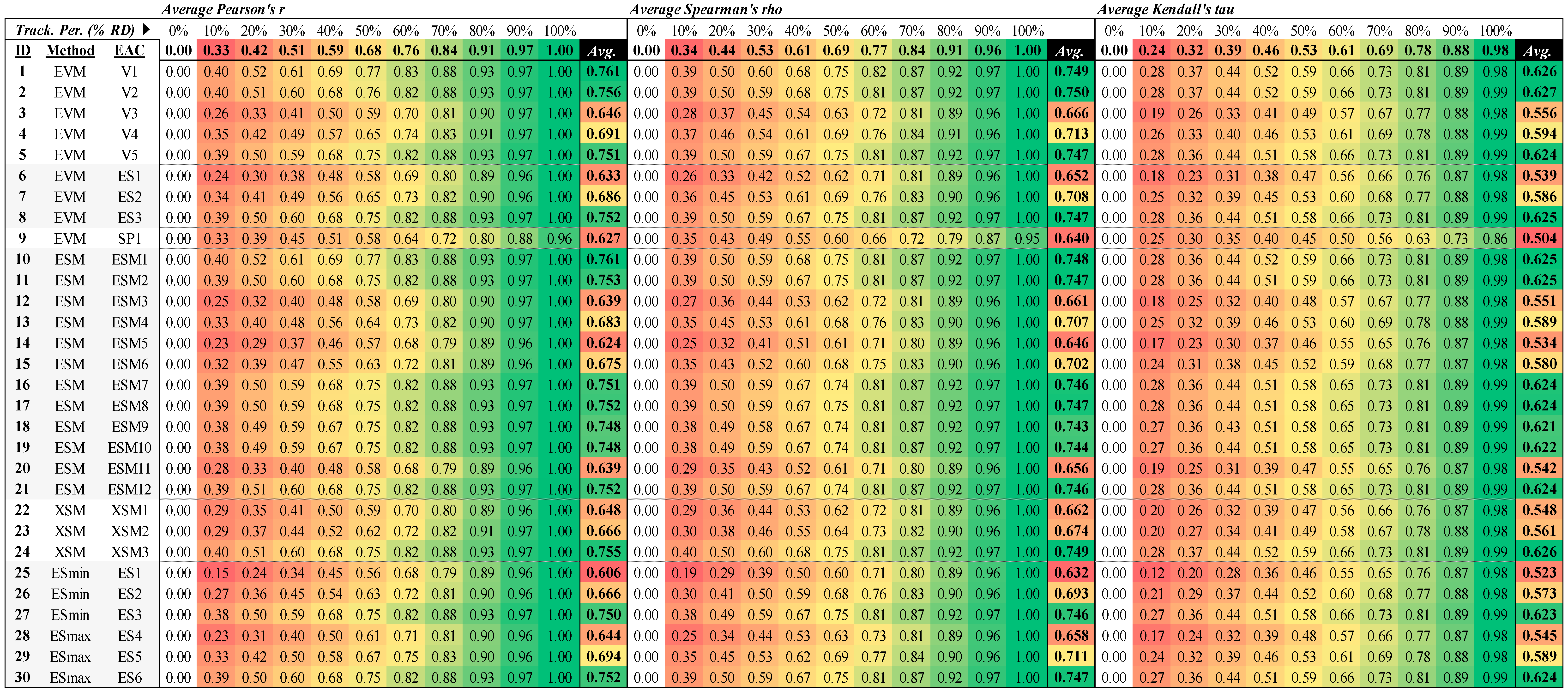
The average stability results (Figure 1) obtained with the three correlation indices are quite consistent with each other, although the values obtained with the Kendall correlation index (τ) are slightly lower than those of the other two correlation coefficients. As described above, the Pearson, Spearman and Kendall correlation values can range between 0 and 1. A value close to “0” implies that the EAC method is unstable (greater volatility of the predictions). A value close to “1” indicates that the method is highly stable (lower volatility).

It is evident that high stability values for the EAC methods are only achieved in the final stage of the project. This result coincides with some recent studies that also compared the stability of EAC methods [45,46]. Considering arbitrarily a correlation value of 80% as the level of correlation from which the correlations are moderately strong, the stability using the methods as determined by the Pearson and Spearman correlation indices would be achieved once approximately 70% of the project has been completed (AT ≥ 70% RD). According to the Kendall correlation index, this threshold of 80% would be achieved somewhat later (AT ≥ 80% RD).

The best methods according to the Pearson correlation index (R) are Methods 1, 2, 8, 10, 11, 21, 24, and 30. In particular, Methods 1, 2, and 10 yield the best results.

The best methods according to the Spearman correlation coefficient (ρ) are Methods 1, 2, 8, 10, 11, 17, 24, and 30. In this case, Methods 1, 2, 10, and 24 are the best.

Finally, the best methods according to the Kendall correlation coefficient (τ) are Methods 1, 2, 5, 8, 10, 11, 24, and 30. Among them, Methods 1, 2, and 24 are the best.

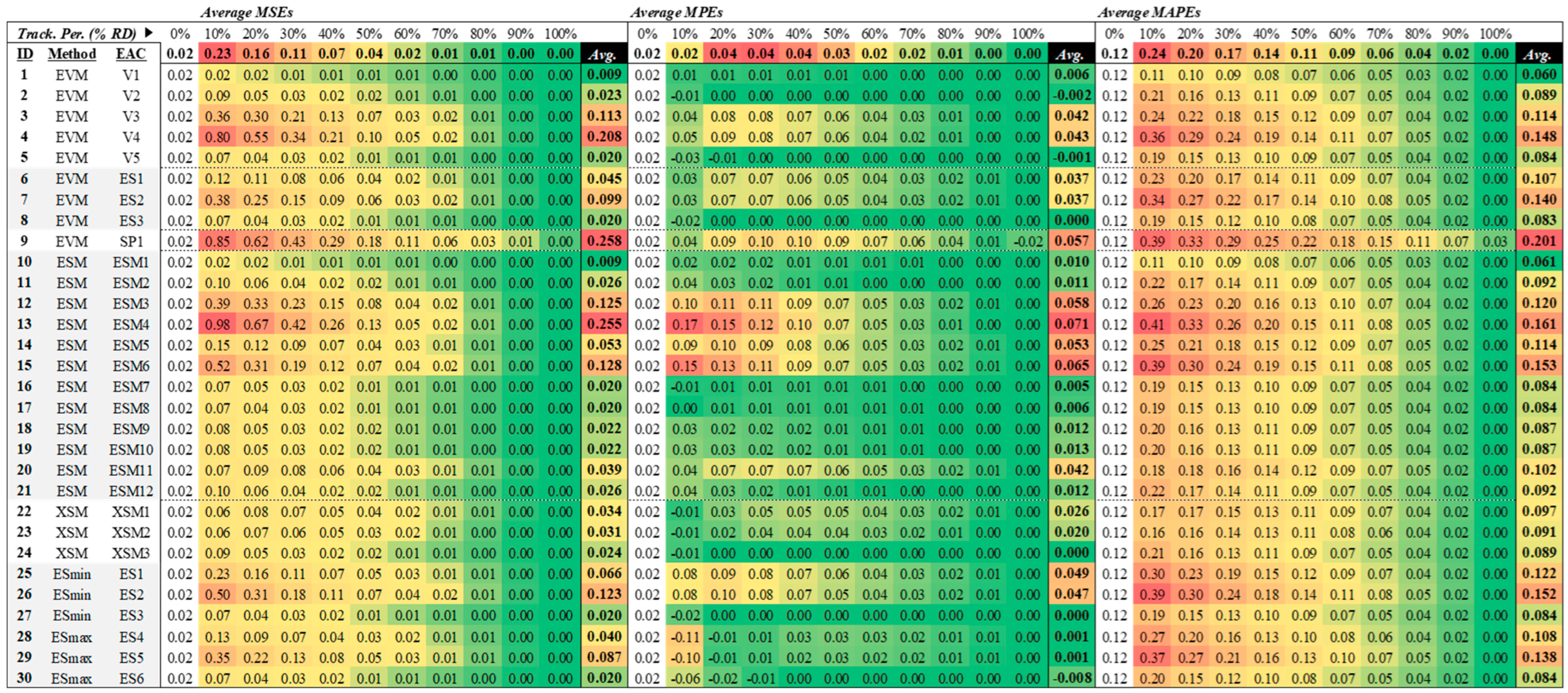
4.2. Accuracy of the EAC Methods

Figure 2 shows the accuracy results of the EAC methods as indicated by the MSE, MPE, and MAPE. As indicated above, a value close to “0” indicates that the method is more accurate (it presents fewer errors when estimating the actual total cost of the project).

Unlike previous studies that highlighted Methods 1, 2, and 9 as the most accurate [3,29,41,43], in our study, we did not obtain the same results. Specifically, according to our analyses, Methods 1, 5, 8, 10, 16, 17, 27, and 30 are the most accurate.

In terms of the accuracy achieved by the EAC methods as a function of the degree of project progress, it is easy to observe that, according to the MSE values, a sufficiently high accuracy is only reached once the project has been half completed (AT ≥ 50% RD). In the last quarter of project execution (AT ≥ 75% RD), the accuracy values are already quite high.

With respect to the results obtained with the MPE values, it is curious to observe that many EAC methods manage to be quite accurate even from the initial stages of project execution. However, it is also observed that many EAC methods tend to underestimate (error metrics with a negative sign) project cost in these initial stages. In contrast, in more advanced stages of the project, the same metrics indicate an overestimation of the project cost (metrics with positive values).

Finally, the results obtained with the MAPE values do not differ much from those obtained with the MSE. That is, in general, at between 50% and 75% of project execution, the percentage errors decrease from 10% to approximately 5%.

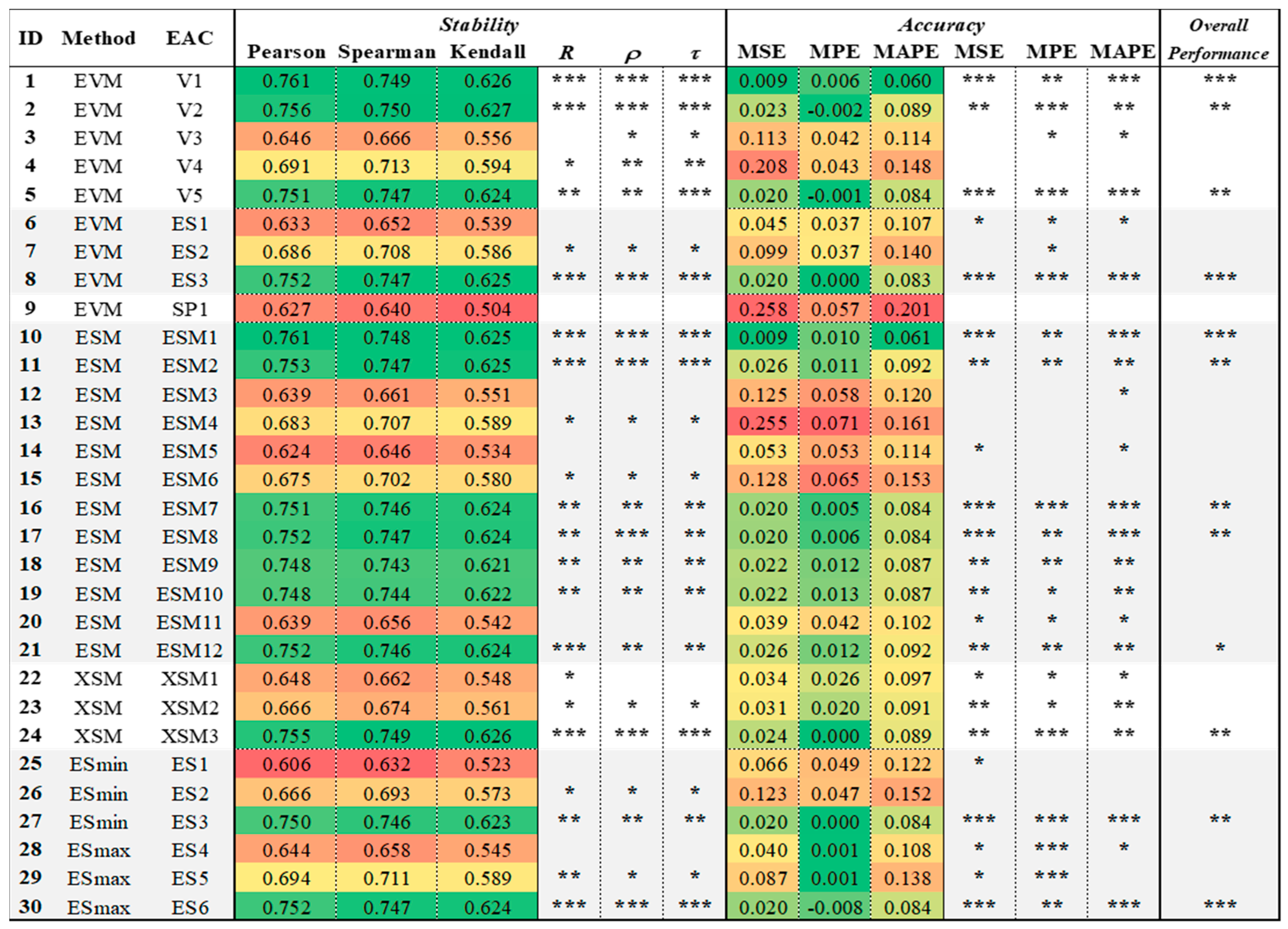
4.3. Summary of Results

The EAC methods with the best results are identified in Figure 3. However, the stability and accuracy results for each of the indicators are found at different scales. It is therefore impossible to directly compare the stability results with the accuracy results. Therefore, we have transformed all the results to a qualitative scale by ordering them from best to worst performance in each of the six metrics used. In this way, the 30 cost prediction methods have been classified into four quartiles, with the position of the quartile indicated using asterisks (“*”). Those prediction methods with “***” are in the first top performing quartile (top eight methods), those with “**” are in the second quartile, those with a “***” are in the third quartile, and those methods without any asterisk are in the fourth quartile. Therefore, more asterisks indicate that the method is better compared to others in terms of its stability or accuracy.

Figure 3 reveals some unexpected results in relation to previous studies. The best four deterministic EAC methods, in terms of both stability and accuracy, are Methods 1, 8, 10, and 30. Methods 1, 8, and 30 adopt the configuration $EAC=AC+\left(BAC-EV\right)/PF$. Method 10 adopts the configuration $EAC=AC+\left(BAC-EV\left(e\right)\right)/PF$. Additionally, Methods 1 and 10 consider a performance factor PF = 1, while Methods 8 and 30 use weighted means to calculate the PF. Specifically, $PF=\alpha CPI+\beta SPI\left(t\right)$ is used in Method 8, and $PF=\alpha CPI+\beta SPI{\left(t\right)}_{ESmax}$ is used in Method 30. Finally, it should be noted that the overall results of Method 1 seem to be slightly higher than those of the others (Methods 8, 10, and 30 included). Therefore, although perhaps only marginally, the simplest formula for estimating the final cost of the project is, paradoxically, the most accurate and stable among all those compared.

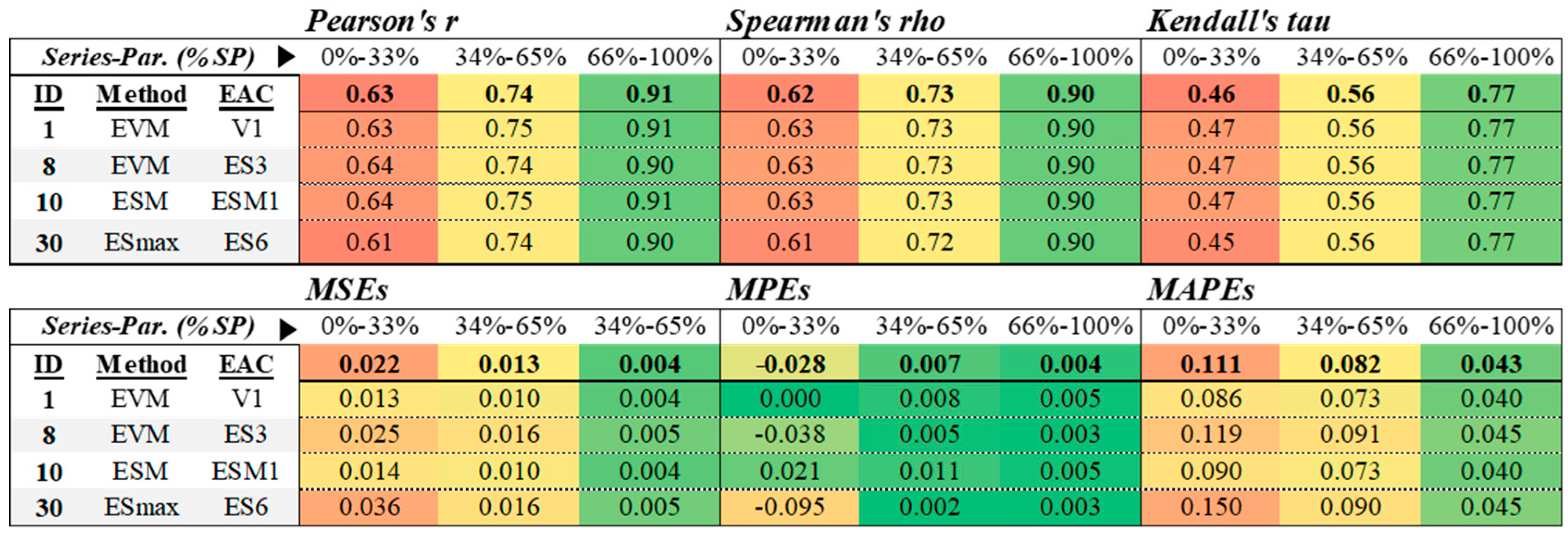
4.4. Consideration of the Project Network Topology

To better discriminate the performance of the best methods in terms of stability and accuracy (Methods 1, 8, 10, and 30), we analyzed their different performances from the perspective of the topological structure of the projects. For this analysis, we calculated the value of the series–parallel (SP) indicator of the 4100 projects used in our analysis. The SP indicator measures the closeness of the structure of a project to a network whose activities are related totally in series (SP = 1) or totally in parallel (SP = 0). In construction projects, the values of the SP indicator usually oscillate between the two extremes, that is, between 0 and 1. As a result, the stability and accuracy of EAC Methods 1, 8, 10, and 30, according to the topological structure of the project, are presented in Figure 4.

Quick inspection of the results of Figure 4 reveals that, both in terms of stability and accuracy, the four cost prediction methods (1, 8, 10, and 30) are much better for projects whose topological structure is closer to that of a series project (% SP values between 66% and 100%) than a project with many parallel paths (% SP between 0% and 33%). This finding agrees with previous results obtained in comparative methods for forecasting project duration [36].

However, although the four methods obtain similar results in terms of their stability (upper half of Figure 4), their accuracy is lower (bottom half of Figure 4). Specifically, Methods 1 and 10 are slightly better than Methods 8 and 30 in terms of their MSE and MAPE values. There is no clear winner in terms of the MPE (some are better than the others as a function of the interval of % SP analyzed). However, Method 1 is still marginally superior to Method 10.

Therefore, according to our analysis, Method 1 stands out as the most accurate and stable as a whole. Because it is also the simplest to calculate, Method 1 seems to be the obvious choice for any project manager who uses EVM and wants to estimate the final cost of the project.

5. Discussion

Only a few previous studies have measured the stability and accuracy of project cost prediction methods using the EVM technique. On the one hand, most studies that measured stability concluded that Method 2 was the most stable from the early stages (approximately AT ≥ 20%, which is the same, i.e., one-fifth of project progress) (e.g., [32,39,42]). However, other studies determined that the stability of the cost prediction methods was not reached before 55%, or even 75%, of project progress [33,44].

The results of our study seem to be more in line with these latter statements. Specifically, in our experiments, we have determined that the EAC methods tend to be much more stable only when the project exceeds approximately 70% of completion. This delayed stability was also reported by other researchers, such as Khrafri et al. [45] and Kim et al. [46]. However, the majority of these researchers considered an EAC method “stable” when its variation was simply less than ±10% of the final value (real cost of the project). In our study, the Pearson, Spearman, and Kendall correlation indices were used to measure stability. The use of these indices provides more representative results and is not subject to any arbitrary threshold (such as the 10% chosen by many researchers). Among the most stable methods, Methods 1, 2, 10, and 24 stood out.

On the other hand, the measurement of the accuracy of an EAC method has been performed by means of three types of errors (MSE, MPE, and MAPE). The results obtained show that the accuracy of the EAC methods is quite high, with the following caveats:

• The accuracy is high when measured from the middle of the project (AT ≥ 50% RD) if the deviations are measured with squared errors (MSE);
• The accuracy is high when measured from early stages (AT ≥ 30% RD) if the deviations are measured with percentage errors (MPE); or
• The accuracy is high when measured late into the project (AT ≥ 80% RD) if the deviations are measured with absolute percentage errors (MAPE).

Based on these apparently disparate results, the following conclusions can be drawn. Apparently, MPE errors become “canceled out” in early and late stages, leading to the belief that EAC methods are more accurate “on average” than they actually are. However, MPE results allow us to know that the EAC methods tend to underestimate the cost of the project in the early stages of the project and that they subsequently tend to overestimate this same final cost.

Additionally, from MSE results, it seems evident that large estimation errors disappear from approximately the middle of the project. Finally, the best estimates will only be obtained in the final fifth of the project (according to the MAPE values). These interpretations of accuracy were not possible in previous comparative studies, since they only used one error metric: the MAPE (e.g., [3,29,41,43]).

Finally, in general terms, monitoring and controlling projects with EAC Methods 1, 8, 10, and 30 should allow project professionals to know the expected cost at the end of the project with greater accuracy and stability. This accuracy and stability will be adequate from the middle of the project but much better in its final stretch (final fifth). With a better estimate of the final cost of the project, project managers will be able to make better decisions regarding the possible reallocation of their work resources. It will also allow them to better understand the budgetary impact of possible time/cost trade-offs in their activities to recover possible delays accumulated during the project.

In terms of the limitations of the present study, 30 EAC methods have been compared using a database of 4100 artificial projects with different topological structures. However, there remains a lack of access to a wide and varied database of real projects to make comparisons. Nevertheless, it is important to note that only with artificial projects is it possible to calculate the stability of EAC methods, because calculating the stability involves simulating possible executions of the same project, which is not possible in real projects that are executed only once. In any case, for future research, it is still necessary to compare the EAC methods in a set of large-scale real projects (hundreds) having topologically varied characteristics. Clearly, this comparison has not been performed, given the difficulty of obtaining such a database.

A last note concerns what would happen when a project applying the cost prediction methods compared here was performed in a market scenario very different to the one that was envisaged during the design stage. Market conditions generally vary over time, but there are also some crisis periods (e.g., high inflation or deflation periods, pandemic confinements, etc.). EVM is a technique that allows correcting the activities’ baseline costs, if necessary. Hence, under scenarios of high price variability, it is not expected that the accuracy and stability results reported in this paper will vary, at least not their performance ranking order.

6. Conclusions

Forecasting the final cost and duration of a project, even approximately, during project execution is essential knowledge for many project management professionals. Such knowledge is more important when there is a high probability of delays and/or cost overruns or when poor performance could negatively affect customer relationships. Having simple techniques to make these predictions is also very useful, especially for project managers without advanced mathematical knowledge.

EVM is a simple technique that allows the final cost and duration of a project to be estimated. By taking advantage of information on project progress in terms of the duration and costs of its activities, EVM can improve the accuracy of its estimates as the project progresses. For this reason, EVM has generated much interest among researchers and project management professionals.

Since EVM was proposed in the 1960s, different extensions of this technique have been proposed to predict the final cost of the project. These extensions, called EACs, started out using mainly the CPI. However, today, EACs adopt other indices whose advantages in terms of accuracy and stability had not yet been exhaustively compared. Additionally, the majority of previous comparisons used a very small number of real projects and/or projects of doubtful representativeness.

To overcome some of these limitations, this study compared the stability and accuracy of 30 deterministic EAC cost prediction methods with a database of 4100 artificial projects whose execution was simulated 100 times each. The stability of the methods was calculated using the Pearson, Spearman, and Kendall correlation coefficients. The accuracy was measured using MPE, MSE, and MAPE. This variety of correlation indices and error metrics has allowed us to better understand how stable and accurate the different EAC methods are and from what point their predictions are sufficiently reliable.

The results of our study differ, in some cases and reinforce, in others, those of several previous studies. Specifically, our results indicate that the cost prediction methods in EVM become quite reliable between 50% and 80% of project execution. The EAC methods that achieve the best results in stability and accuracy are Methods 1, 8, 10, and 30, with Method 1 being marginally superior to the other three. The formulations of these methods follow a fairly simple mathematical structure. Specifically, the expression of Method 1 is $EAC=AC+BAC-EV$, where AC is the actual cost incurred to date in the execution of the project, BAC is the budgeted total cost of the project, and EV is the earned value cumulated by the project to date.

Comparing the stability and accuracy of the EAC methods will allow project professionals to, first, know which methods are the most reliable in terms of predicting the final cost of their projects; second, make better preventive decisions that allow resources to be redistributed more efficiently among those activities that add value; third, make better corrective decisions throughout the project life cycle to reduce the total actual costs of the activities in progress or to be executed; and fourth, develop a consistent calculation framework that also allows comparison with other EAC extensions proposed in the future.