Performance of Six Metaheuristic Algorithms for Multi-Objective Optimization of Nonlinear Inelastic Steel Trusses

Abstract

This paper presents a multi-objective optimization of steel trusses using direct analysis. The total weight and the inter-story drift or displacements of the structure were two conflict objectives, while the constraints relating to strength and serviceability load combinations were evaluated using nonlinear inelastic and nonlinear elastic analyses, respectively. Six common metaheuristic algorithms such as nondominated sorting genetic algorithm-II (NSGA-II), NSGA-III, generalized differential evolution (GDE3), PSO-based MOO using crowding, mutation, and ε-dominance (OMOPSO), improving the strength Pareto evolutionary algorithm (SPEA2), and multi-objective evolutionary algorithm based on decomposition (MOEA/D) were applied to solve the developed MOO problem. Four truss structures were studied including a planar 10-bar truss, a spatial 72-bar truss, a planar 47-bar powerline truss, and a planar 113-bar truss bridge. The numerical results showed a nonlinear relationship and inverse proportion between the two objectives. Furthermore, all six algorithms were efficient at finding feasible optimal solutions. No algorithm outperformed the others, but NSGA-II and MOEA/D seemed to be better at both searching Pareto and anchor points. MOEA/D was also more stable and yields a better solution spread. OMOPSO was also good at solution spread, but its stability was worse than MOEA/D. NSGA-III was less efficient at finding anchor points, although it can effectively search for Pareto points.

1. Introduction

Steel truss structures with lightweight properties, efficient use of materials, and various shapes have been widely used in civil and industrial works. Due to the nonlinear inelastic behavior of steel structures, steel trusses should be designed by using nonlinear inelastic analyses, which have recently been accepted by major standards such as Eurocode [1] and AISC LRFD [2]. In nonlinear inelastic analyses, the boring and complicated separate check of every structural member in member-based analysis methods has simply been replaced by using the ultimate load-carrying capacity of the whole structure. Furthermore, the nonlinear inelastic behavior, failure mode, overall buckling, and member interaction of the whole system were directly assessed. Some highlight studies regarding this topic can be reviewed in [3,4,5], among others.

To improve the quality of the truss design solutions, optimization approaches have been studied extensively for more than three decades. The most common problem is single-objective optimization (SOO), where only one objective function is considered under several constraints to ensure normal working conditions (for example, [6,7,8]). The objective function is often chosen as the minimization of the total weight/cost of the whole structure with continuous or discrete design variables. Due to the several nonlinear aspects such as complicated search spaces, non-convex feasible regions, structural nonlinear behaviors, etc., metaheuristic algorithms have been widely used that can better find global optimal solutions [9,10,11,12]. A common characteristic of metaheuristics algorithms is that they provide good optimum results but not optimal solutions, and spend abundant structural analyses to evaluate the constraints. Computation efforts of structural optimization using nonlinear analysis become too excessive since nonlinear analysis is much slower than linear analysis. In light of this, the number of studies on truss optimization using nonlinear inelastic analysis is still small. Some of the prominent studies are in [13,14,15,16,17].

It should be noted that the actual design works often have more than one objective function to satisfy several requirements both in terms of the cost and technical aspects. Normally, such a problem can simply be solved by converting them into an SOO using weighted methods or by considering the considered objective functions as constraints. However, weighted methods are not effective in some cases, especially when the objectives are conflicted and a trade-off among the objectives is required. For example, the cost minimization objective often conflicts with the maximization of structural safety and serviceability objectives. In addition, the methods considering objective functions as constraints, namely, letting them receive specific values, can find only one optimal solution for each optimization run. Therefore, these approaches may require excessive computational efforts to find the realistically optimal solution set of a multi-objective optimization (MOO) problem. As a consequence, aside from SOO, MOO, which simultaneously considers two or more objective functions, has attracted significant interest from researchers. Unlike SOO, where only one optimal solution is found, MOO, in principle, provides a group of solutions, called Pareto optimal solutions or non-dominated solutions. Therefore, the main goal of the MOO is to search for as many non-dominated solutions as possible. Mahrach et al. [18] presented a comparison between single and multi-objective evolutionary algorithms to solve the Knapsack Problem and the Travelling Salesman Problem. The results prove that the direct application of a multi-objective solver to a MOO problem is much better than transforming the MOO problem into an SOO one. In light of this, many multi-objective optimization algorithms based on evolution have been proposed such as the strength Pareto evolutionary algorithm (SPEA) [19], vector evaluated genetic algorithm (VEGA) [20], Pareto-archived evolution strategy (PAES) [21], and nondominated sorting genetic algorithm-II (NSGA-II) [22], among others. The efficiency of evolutionary multi-objective optimization algorithms (EMOA) has been proven through their successful application in many fields such as composite structures [23], structural damage detection [24], reinforced concrete structures [25], buildings [26], etc.

Regarding the MOO of truss structures, several interesting studies have been published in the literature. Eid et al. [27] proposed a multi-objective water cycle algorithm (MOWCA) and demonstrated its efficiency through bi-objective optimization of three benchmark trusses including 10-bar, 25-bar, and 200-bar trusses. Gholizadeh et al. [28] developed multiobjective uniformly distributed particles (MO-UDPs) for the multi-objective optimization of steel moment frames under seismic loading, which was proven using two benchmark 10-bar and 25-bar trusses. Kaveh and Ghazaan [29] introduced a multi-objective variant of the vibrating particle system (MOVPS) and used a 120-bar dome-shaped truss and a 582-bar tower truss as two case studies for verification. Ho-Huu et al. [30] proposed a framework for reliability-based MOO of trusses using NSGA-II. The case studies were three benchmark truss optimization problems including 10, 25, and 120 bars. Lemonge et al. [31] used the third evolution step of generalized differential evolution (GDE3) to the MOO of truss structures considering the natural frequencies of vibration and global stability. More studies on the MOO of truss structures are presented in [32,33,34,35,36,37], among others. The above studies show the effectiveness and potential of applying MOO to truss design. However, the number of truss MOOs is much less compared to that of SOO. Furthermore, the published works only focused on linear trusses through benchmark case studies. Studies on the effectiveness of MOO for nonlinear truss structures are a gap in the literature. Furthermore, the publications utilized different MOO methods with most based on evolutionary algorithms. As a consequence, an important question still needs to be answered about the effectiveness of such algorithms for unstudied optimization problems such as nonlinear inelastic truss structures.

In this study, the multi-objective optimization of steel trusses using nonlinear inelastic analysis was developed. Two conflict objectives such as the total weight and the inter-story drift or displacements were considered. The constraints were set according to the strength and serviceability load combinations which are evaluated using direct analysis. Six efficient and popular metaheuristic algorithms such as NSGA-II, NSGA-III, GDE3, PSO-based MOO using crowding, mutation, and ε-dominance (OMOPSO), improving the strength Pareto evolutionary algorithm (SPEA2), and multi-objective evolutionary algorithm based on decomposition (MOEA/D) were employed to solve the developed MOO problem. Four truss structures were studied including a planar 10-bar truss, a spatial 72-bar truss, a planar 47-bar powerline truss, and a planar 113-bar truss bridge. The rest of this paper is organized as follows. The MOO problem of nonlinear inelastic trusses is formulated in Section 2. Section 3 overviews the considered MOO algorithms. Four examples of truss optimization are presented in Section 4, and Section 5 presents some of the conclusions drawn from this work.

2. Multi-Objective Optimization Problem Formulation of Nonlinear Inelastic Trusses

2.1. Nonlinear Inelastic Analysis of Truss Structures

The nonlinear inelastic analysis of truss structures was performed by dividing the applied loading into many small increments. The structural responses and deformation were memorized consecutively. In this way, the nonlinear relationship of force–displacement was directly captured, which was used to determine the ultimate load-carrying of the whole structure. For simplicity, the ultimate load factor (ULF), which is the ratio between the ultimate load-carrying capacity (R) and applied loading (S), was used instead of the ultimate load-carrying capacity. The structural safety was satisfied when ULF was not smaller than 1.0 and in contrast. As a consequence, a trivial safety check of every structural member in the linear analysis was eliminated.

To include the nonlinear behavior of truss elements, the stress–strain constitutive model proposed by Blandford [38] was utilized, which is presented in Figure 1. As can be seen in this figure, Blandford’s model includes all major modes such as compression, elastic and inelastic post-buckling, inelastic post-buckling unloading, tension, post-yielding, and tension unloading. The detailed equations for these curves can be found in [38].

The nonlinear equilibrium equation for a truss element is as follows, using an incremental form developed by Yang and Kuo [39]:

$$\left(\left[k_E\right]+\left[k_G\right]+\left[s_1\right]+\left[s_2\right]+\left[s_3\right]\right)\left\{d\right\}+{}^{1}f={}^{2}f$$

(1)

where ¹f and ²f are forces acting on the two nodes at the previous and current states, respectively; [k_E] and [k_G] are the elastic and geometric stiffness matrices, respectively; and [s₁], [s₂], and [s₃] are higher-order stiffness matrices to consider the nonlinear part of the axial strain. To solve Equation (1), the generalized displacement control (GDC) method [40], which efficiently calculates the equilibrium path of nonlinear structures with multiple limit points and snap-back, is employed. The aforementioned nonlinear truss model and GDC algorithm were utilized in the Practical Advanced Analysis Program (PAAP) [41]. This program was used to perform nonlinear inelastic analysis of truss structures in this study.

2.2. Statement of Multi-Objective Optimization of Trusses Using Nonlinear Inelastic Analysis

In a multi-objective optimization problem, at least two mutually conflicting objectives are considered. Commonly, to reflect the economic efficiency of the proposed design, the total cost or weight of the structure is selected as an objective function in structural optimization. In light of this, the cross-sections of structural members are designed to reach the minimum total cost/weight of the structure, while all design requirements are still satisfied including the strength, serviceability, and constructability conditions. However, minimizing the total cost/weight of the structure tends to use smaller cross-sections of structural members that may significantly reduce the stiffness of the structure, in other words, reduce the structural safety. To enhance the structural performance, the maximum inter-story drift or lateral displacement has been considered the second objective function in the MOO problems of truss structures [30,31,34]. By minimizing the maximum inter-story drift/lateral displacement, the global structural stiffness was increased. The above objectives are the two basic objectives in the design of the structure that were also taken into account in this study. It should be noted that several aspects of the structural design may be considered objective functions such as the smallest load-carrying capacity, natural frequencies, number of different cross-section types, failure probability, etc. The considered MOO problem for the sizing optimization of trusses using nonlinear inelastic analysis with continuous design variables is written as follows:

$$\mathrm{Objective} \mathrm{function} 1: \mathrm{Minimize}:\hspace{1em}\hspace{1em}\hspace{1em}{F}_1\left(\mathrm{X}\right)={\displaystyle \sum _{i=1}^N{\rho }_i{X}_i{L}_i}$$

(2)

$$\mathrm{Objective} \mathrm{function} 2: \mathrm{Minimize}: F_2\left(\mathrm{X}\right)=\sqrt{{\displaystyle \sum _{j=1}^{N_{story}}{\left(d_{k,j}\right)}^2}} k=1,..,N_{\mathit{service}}$$

(3)

where i, j, and k are the numerical orders of structural members, structural stories, and serviceability load combinations considered, respectively; ρ, L, and X are the material weight density, member length, and member cross-sectional area, respectively; N_service is the number of serviceability load combinations considered; d_k,j is the inter-story drift of the jth story in the kth serviceability load combination. It should be noted that the second objective function in Equation (2) can be presented in the form of nodal displacements of the truss.

The first constraint of the considered optimization problem is the value range for continuous design variables, which are written as

$$A_i^{lowb}\le X_i\le A_i^{upb}$$

(4)

where $A_i^{lowb}$ and $A_i^{upb}$ are the lower- and upper-bounds of the ith design variable. The next constraints are strength constraints that correspond to the strength load combinations required by design standards. In light of nonlinear inelastic analysis, the structural safety is simply checked by comparing the overall load-carrying capacity of the structure R with the applied loading S. Therefore, the strength constraints are as follows:

$$C_l^{strength}=1-\frac{R_l}{S_l}=1-UL{F}_l\le 0 l=1,..,N_{strength}$$

(5)

where N_strength is the number of the strength load combinations considered. Corresponding to the serviceability load combinations, the inter-story drifts of the structure are guaranteed through the following equation:

$$\mathrm{Subject} \mathrm{to}: C_{n,j}^{service}=\frac{\left|d_{k,j}\right|}{d_{k,j}^u}-1\le 0 k=1,..,N_{\mathit{service}}; j=1,..,N_{story}; n=1,..,N_{service}$$

(6)

where N_service is the number of serviceability load combinations considered and $d_{k,j}^u$ is the allowable value of the inter-story drift of the jth story in the kth serviceability load combination d_k,j. In the case the second objective function is presented in the form of nodal displacements, Equation (6) will also be expressed as nodal displacements.

For constraint handling, the penalty function method was employed in this study since this method is simple and easy to use. The objective functions presented in Equations (2) and (3) can be rewritten as

$$F_1^{un}\left(\mathrm{X}\right)=\left(1+{\displaystyle \sum _{l=1}^{N_{strength}}{\alpha }_{str,l}{\beta }_{1,l}}+{\displaystyle \sum _{n=1}^{N_{\mathit{service}}}{\alpha }_{disp,n}{\beta }_{2,n}}\right)\times F_1^{}\left(\mathrm{X}\right)$$

(7)

$$F_2^{un}\left(\mathrm{X}\right)=\left(1+{\displaystyle \sum _{l=1}^{N_{strength}}{\alpha }_{str,l}{\beta }_{1,l}}+{\displaystyle \sum _{n=1}^{N_{\mathit{service}}}{\alpha }_{disp,n}{\beta }_{2,n}}\right)\times F_2^{}\left(\mathrm{X}\right)$$

(8)

$$\mathrm{where}: {\beta }_{1,l}=\max \left(C_l^{strength},0\right);{\beta }_{2,n}={\displaystyle \sum _{j=1}^{N_{story}}\max \left(C_{n,j}^{service},0\right)}$$

(9)

where α_str,l and α_disp,n are the pre-defined penalty parameters chosen with large values to remove the unfeasible candidates in the optimization process. In this study, the penalty parameters were equal to 10,000.

3. Description of Multi-Objective Optimization Algorithms

3.1. Short Review of MOO Algorithm Development

To solve MOO problems, several methods have been developed in the literature that can be classified into three big categories: (1) transforming into an SOO problem by combining the individual objective function; (2) transforming into a single objective optimization by keeping only one objective and moving others to the constraint set; (3) finding the entire Pareto optimal solutions. In the first approach, the weighted sum method is employed by using the weighting coefficients w_i with Σw_i = 1. By changing the values of w_i, many SOO problems were developed where one Pareto optimal solution could be found corresponding to each SOO problem. An SOO problem is now simply solved by using metaheuristic SOO algorithms, for example, differential evolution (DE) [42], genetic algorithm (GA) [43], harmony search (HS) [44], etc. However, this approach still has several limitations such as (1) requiring more computational efforts compared to using MOO algorithms; (2) it is not easy to find the best form of weighted sum function since there are too many ways to construct it; (3) changing the values of the weighting parameters does not ensure finding good Pareto front points since the same or very close points are found. Furthermore, the weighted sum method is not efficient in the case of a nonconvex objective space.

In the second approach, only one objective function is kept while the remaining are moved to the constraint set. The MOO problem is now converted into several SOO problems by changing the constraining values for moved objective functions. However, this approach seems rather arbitrary in choosing constraining values that should be carefully chosen so that they are in the minimum and maximum values of the corresponding objective function. Furthermore, this approach has similar limitations as the first approach, although it works well with nonconvex objective spaces.

In the third approach, the entire Pareto optimal solutions or Pareto front are found simultaneously thanks to metaheuristic algorithms for this type of problem called MOO algorithms. Metaheuristic algorithms such as evolutionary algorithms deal with a population of promising solutions, so they are potentially suitable for finding Pareto optimal solutions to a MOO problem with only a single run. Furthermore, metaheuristic algorithms based on stochastic searching techniques are efficient in finding globally optimal solutions to highly nonlinear and non-convex optimization problems. In light of this, the current work focused on MOO metaheuristic algorithms including NSGA-II, NSGA-III, GDE3, OMOPSO, SPEA2, and MOEA/D. The main content of each algorithm is presented in the following sections.

3.2. Nondominated Sorting Genetic Algorithm-II (NSGA-II)

NSGA-II was proposed by Deb et al. [22] in 2002. It is an improved version of NSGA introduced by Srinivas and Deb in 1995 [45], which is considered as one of the first MOO methods based on evolutionary algorithms (EA). Basically, NSGA-II follows the general outline of a GA inspired by Darwin’s evolutionist theory. In GA, the individual or chromosome of the next population is created from the “good” parents, which are the individuals/chromosomes of the current population through three basic techniques including mutation, crossover, and selection. In the traditional GA version, an individual or chromosome is presented in binary form with many discrete units called genes, having values of 1 or 0. The process of producing a child/offspring starts by choosing two chromosomes/parents from the current population using a selection process such as roulette wheel selection, event selection, rank-grounded selection, etc., in order to find the better parents from the current population. Then, in the crossover process, parents are combined by swapping genetic information. Some typical crossover techniques are one-point crossover, two-point crossover, etc. The mutation operator is applied at a very small rate by changing the values of some genes in the offspring to prevent premature convergence to the local optima. To maintain the solution quality obtained in the optimization process, the “elitist selection” technique is usually employed, which allows keeping the best individual of the current population to the next one.

In light of GA, NSGA-II was developed to solve MOO problems with two key aspects including fast nondominated sorting and crowded comparison to sort individuals. A fast nondominated sorting is used to sort individuals into different non-domination fronts using two entities: (1) domination count n_t, which is the number of solutions dominating the solution p, and (2) S_p, which is a set of solutions that the solution p dominates. This approach can save the computational costs for sorting the population into nondomination levels in the optimization process. The crowded comparison is a selection mechanism based on two factors: (1) nondomination rank and (2) crowding distance. A solution is defined as better than another if it is on lower nondomination ranks or located in a lesser crowded region in the case they are in the same front. The common crossover and mutation operators used in NSGA-II are simulated binary (SBX) and polynomial, respectively, which can be found in the [46] and [47]. More details of NSGA-II are given in [22].

The main steps of NSGA-II are as follows:

Step 1: Randomly create an initial population.

Step 2: Sort the population using fast nondominated sorting and crowding distance techniques.

Step 3: Choose parents using the binary tournament selection using the crowded-comparison operator.

Step 4: Create offspring using simulated binary crossover and polynomial mutation.

Step 5: Offspring and current populations are combined to fill the new population from better fronts. Crowding distance is used for individuals in the same front.

3.3. Nondominated Sorting Genetic Algorithm-III (NSGA-III)

The numerical results in the literature prove the efficiency of NSGA-II to solve multi-objective optimization problems with two or three objective functions. However, NSGA-II faces great difficulties when the number of objective functions increases due to the existence of dominance-resistant individuals. The characteristics of dominance-resistant individuals are that they are good at some objectives, but also bad at several others. On one hand, with some very bad objective values, they are far away from the Pareto front. On the other hand, they are difficult to dominate by other individuals since they have some very good objectives. In addition, with their very bad objective values, they are far away from other individuals, which allows them to have a good crowding distance. Therefore, they can survive over several generations, or the convergence speed of NSGA-II is severely affected.

To overcome the above-mentioned drawbacks of NSGA-II, Deb and Jain proposed NSGA-III in 2014 [48]. The basic framework of NSGA-III is similar to NSGA-II with new selection operator techniques in order to solve many-objective problems. In NSGA-III, instead of using the crowding distance as in NSGA-II, reference points are used to maintain the diversity of the population. Commonly, the Das–Dennis method is employed to uniformly sample reference points on a normalized hyper-plane. In this method, an (M-1) dimensional normalized hyper-plane was created first, where M is the number of objectives. Along each objective, p divisions are considered that form a total of reference points $H=\left(\begin{array}{c}M+p-1\\ p\end{array}\right)$. The widely distributed reference points make the obtained individuals likely to be widely distributed on or near the Pareto-optimal front. A niche-preservation operation was developed to select the individuals on the same front. The brief procedure of this operation is as follows. First, a new population S_t is constructed including the individuals from the first front F₁ to the lth front F_l while the size of S_t is first greater or equal to the defined size of the optimization population N. Second, each individual in S_t\F_l is associated with a reference point having the minimum perpendicular distance. The individuals in F_l are chosen in light of filling up the underrepresented reference directions. If the reference direction does not have any individual specified, the individual with the smallest perpendicular distance is selected. If a second individual is added to this reference line, it is chosen randomly from the remaining individuals in F_l. The details of NSGA-III can be found in [49].

3.4. Generalized Differential Evolution 3 (GDE3)

GDE3 was developed by Kukkonen and Lampinen [50] in 2005, which is an expanded version of DE, one of the most popular metaheuristic algorithms for solving MOO problems. The mutation technique DE/rand/1/bin proposed in the traditional DE algorithm is used in GDE3 to generate the trial vectors. Then, the new population is filled up by using the following selection operation:

(1)

If both the trial vector U and target vector X are infeasible, U will be chosen if it weakly dominates X in the constraint violation space and otherwise;

(2)

If only one vector in U and X is feasible, it will be chosen;

(3)

If both U and X are feasible, U will be chosen if it weakly dominates X in the objective function space and otherwise.

In light of the above selection operation, the size of the population after a generation of GDE3 is in the range [NP, 2NP] that will be decreased to a NP size by using the fast nondominated sorting and crowding distance proposed in NSGA-II. The details of GDE3 can be found in [48].

3.5. PSO-Based MOO Using Crowding, Mutation, and ε-Dominance (OMOPSO)

OMOPSO was introduced by Reyes and Coello [51] in 2005. This algorithm is an improved version of the well-known SOO algorithm PSO for MOO problems. Basically, OMOPSO is based on the Pareto dominance and crowding value for the selection of leaders. For each individual/particle, the leaders are selected by using a binary tournament in light of their crowding values. The leaders are stored in an external archive with a size equal to the size of the population/swarm. After each generation, this set is updated with new crowding values of the stored leaders. If the size of the set is greater than the defined size, the best leaders are kept based on their crowding values.

For mutation operation, three types are proposed in OMOPSO including (1) uniform mutation; (2) non-uniform mutation; (3) not using mutation. Uniform and non-uniform mutations are used to modify the values of the decision variables of a particle with a certain probability. A scheme was developed, allowing the swarm to be divided into three equal parts, which was applied to the three above different types in order to achieve the exploration and exploitation abilities of the uniform and non-uniform mutations, respectively. The mutation probability is equal to 1/codesize, where codesize is the total length of the string for encoding all variables.

The ε-dominance is employed to fix the size of another external, which is used to contain the non-dominated solutions (final solutions). In this approach, an individual dominates (or ε-dominate) X₂ if f_i(X₁)/(1 + ε) ≤ f_i(X₂) with all objectives and f_i(X₁)/(1 + ε) ≤ f_i(X₂) for at least one objective. The value of ε is predefined by users and is the same for all objective functions.

3.6. Improving the Strength Pareto Evolutionary Algorithm (SPEA2)

SPEA2 developed by Zitzler et al. [52] is the improvement of SPEA proposed by Zitzler and Thiele [53] with three basic strategies including an enhanced archive truncation, a fine-grained fitness assignment, and a density estimation. At the beginning of the optimization process, an empty external archive Q is created, along with the population P. Each individual i in both P and Q is assigned a strength value S(i), which is then the number of solutions in (P ∪ Q) dominated by or equal to i. The fitness $F\left(i\right)$ of i is calculated as

$$F\left(i\right)=\left({\displaystyle \sum _{j\in P\cup Q,j\Phi i}S\left(j\right)}\right)+\left(\frac{1}{{\sigma }_i^k+2}\right)$$

(10)

where jϕi means the individual j dominates or is equal to the individual i. The distances in the objective space of the individual i to all individuals j in P and Q are sorted in increasing order to find the k-th element, which is denoted as ${\sigma }_i^k$ with $k=\sqrt{size(P)+size(Q)}$.

The archive Q is updated as follows: (1) take all nondominated individuals having F(i) < 1 from P and Q to the archive of the next generation; (2) if quantity is not enough, the remaining is taken from the best-dominated individuals in P and Q; (3) if the quantity is too large, a truncation strategy is employed to remove the individuals having the minimum distance to another individual in the archive.

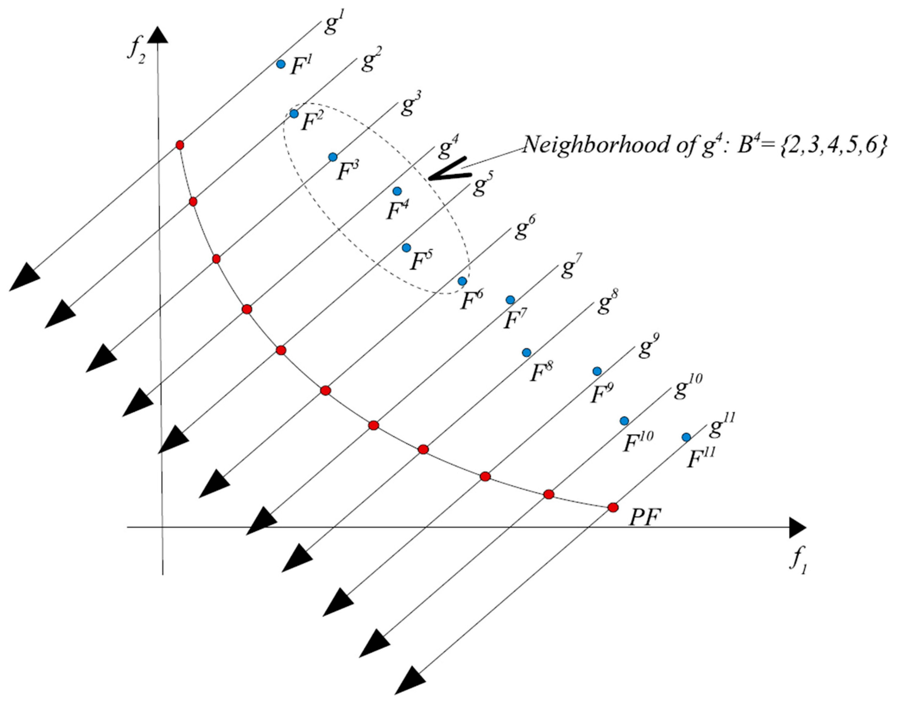
3.7. Multi-Objective Evolutionary Algorithm Based on Decomposition (MOEA/D)

MOEA/D or MOEAD was developed based on evolutionary algorithms (EA) and decomposition [54]. In fact, MOEAD is a framework that allows the use of several evolutionary operators such as DE crossover and mutation strategies. The most innovative MOEAD is to decompose a MOO problem into several SOO sub-problems that are solved simultaneously and cooperatively to find and combine good solutions of neighboring problems, which are expected to be Pareto points, as illustrated in Figure 2. A sub-problem is solved primarily using information from its neighboring ones.

The weighted Tchebycheff approach, one of the famous decomposition methods, can be used to decompose a MOO problem, since it can effectively handle problems with non-convex Pareto fronts. Note that this approach often only works well with MOO problems with normalized objective functions. The simple normalization method uses the ideal point $z_{}^{*}=\left(z_1^{*},z_2^{*},..,z_m^{*}\right)$ where $z_i^{*}$ is the optimum value of the objective i-th as follows:

$$f_i^{\prime }\left(\mathrm{x}\right)=f_i^{}\left(\mathrm{x}\right)-z_i^{*}$$

(11)

4. Numerical Examples

Four steel trusses (planar 10-bar, spatial 72-bar, 47-bar power line, and 113-bar planar bridge) are discussed in this section. The design variables were the member cross-sectional areas, which were continuous in the range [645.16, 6451.6] (mm²) in the first three cases and [3870.96, 22580.6] (mm²) in the last case study. The steel material was A992 with an elastic modulus of 200 (GPa) and a yield strength of 344.5 (MPa). Considered algorithms were developed using the programming language Python with the system parameters presented in

Table 1. Optimization algorithm parameters.

Algorithm	Parameter Value
NSGA-II	offspring_population_size = 1; crossover = SBXCrossover (probability = 0.9); mutation = Polynomial_Mutation (probability = 1.0/number_of_variables); tournament selection
NSGA-III	Uniform Reference Points = Population size—1; crossover = SBXCrossover (probability = 0.9); mutation = PolynomialMutation (probability = 1.0/number_of_variables)
GDE3	CR = 0.9; F = 0.1; DE/rand/1
OMOPSO	epsilon = 0.0075; leaders = Crowding_Distance_Archive (100) Uniform_Mutation (probability = 1.0/number_of_variables, perturbation = 0.5); Non_ Uniform_Mutation(probability = 1.0/number_of_variables, perturbation = 0.5)
SPEA2	offspring_population_size = population_size; crossover = SBXCrossover (probability = 1.0); mutation = Polynomial_Mutation (probability = 1.0/number_of_variables)
MOEA/D	crossover = Differential_Evolution_Crossover (CR = 1.0, F = 0.5); mutation = Polynomial_Mutation (probability = 1.0/number_of_variables); aggregative_function = Tschebycheff (dimension = number_of_objectives); neighbor_size = 20; neighbourhood_selection_probability = 0.9; max_number_of_replaced_solutions = 2

, which were chosen by using trial-and-error to find suitable values. The population size was equal to 100 in all cases. The number of iterations was 200 for the first case study and 300 for the three remaining case studies. Each algorithm was run 10 independent times to minimize the effect of stochastic characteristics in the metaheuristic algorithms. The PAAP program [41] was employed to perform nonlinear inelastic analysis of the steel truss structures. All applied loads were converted into concentrated loads at structural nodes. To evaluate the performance of MOO algorithms, four indicators were used including generational distance (GD), generational distance plus (GD+), inverted generational distance plus (IGD+), and hypervolume (HV). The GD indicator measures the distance from optimal solutions to the Pareto-front, which is later improved by using GD+ through modifying the distance. IGD+ measures from any point in the Pareto-front to the closest point in the optimal solution set. The HV indicator measures the volume of the dominated area formed by the optimal solutions and a reference point. With the above definition, the better algorithm will have smaller values of GD, GD+, and IGD+ and higher values of HV. Detailed equations of these indicators can be found in [35].

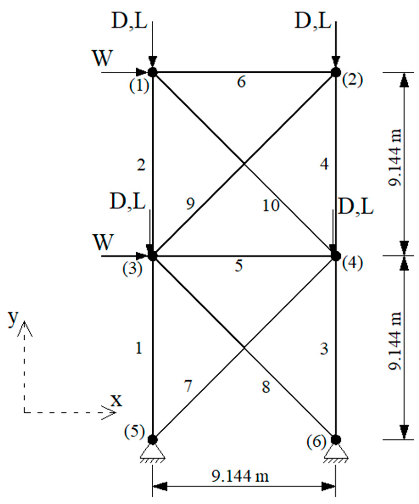
4.1. Planar 10-Bar Truss

A 10-bar planar truss with the layout and geometry in Figure 3 was studied in this section. The number of design variables was 10. The dead load (D), live load (L), and wind load (W) were equal to 150, 100, and 100 (kN), respectively. Two strength and one serviceability load combinations were considered including 1.2D + 1.6L, 1.2D + 0.5L + 1.7W, and 1.0D + 0.5L + 0.7W, respectively. The allowable drift is h/400, where h is the story height of the truss. 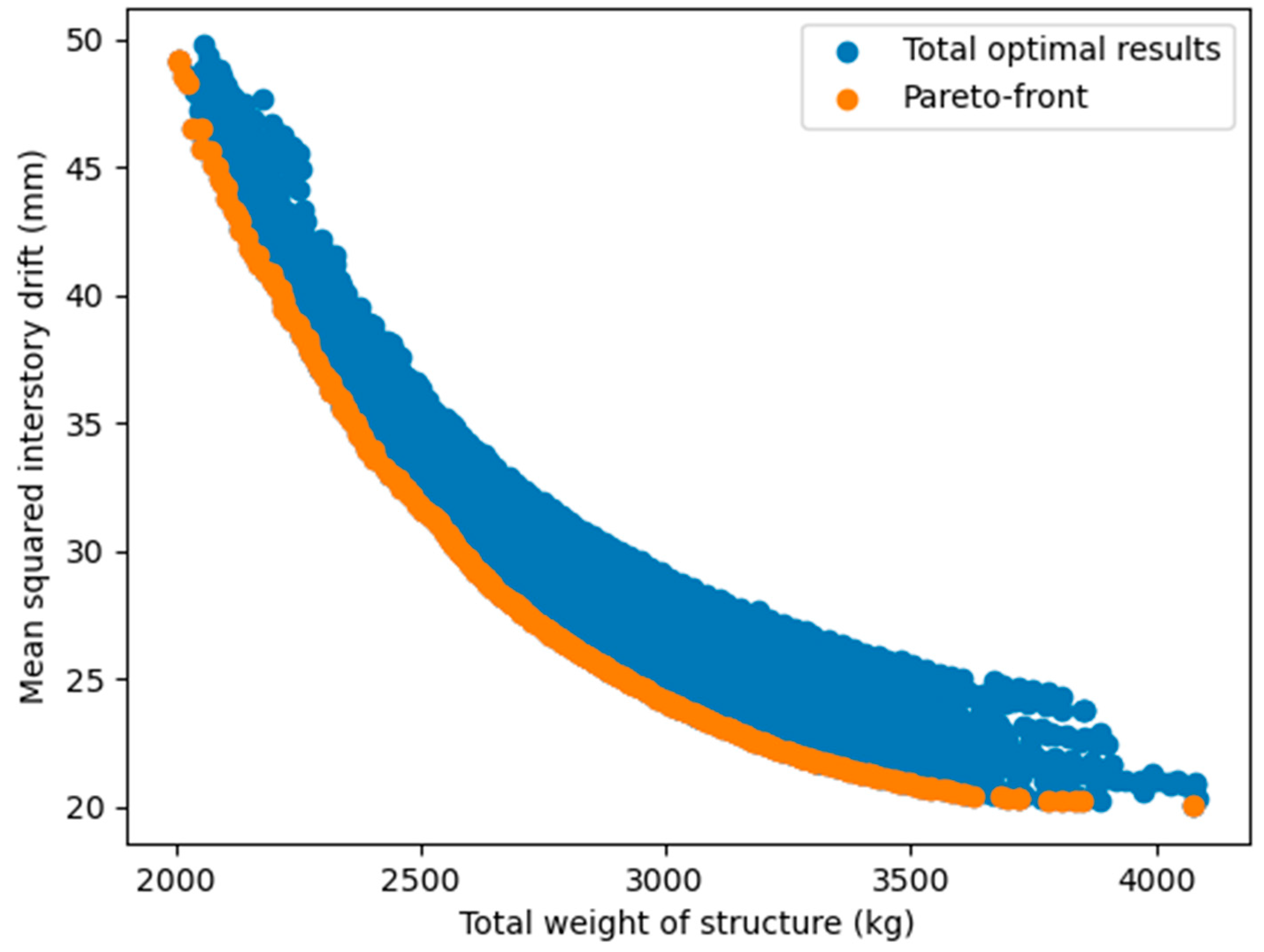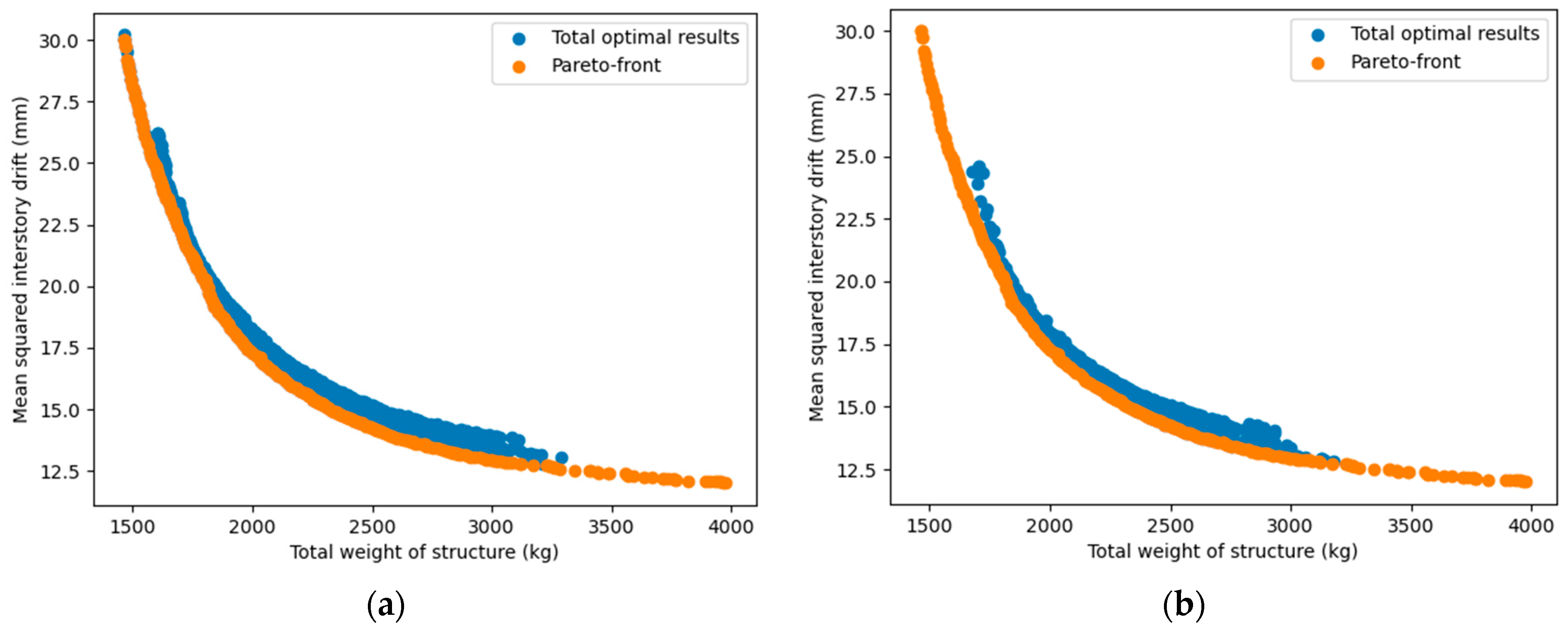The first objective is the total weight of the structure and the second objective is $F_2\left(\mathrm{X}\right)=\sqrt{x_1^2+x_3^2}$, where x₁ and x₃ are the horizontal displacements of nodes 1 and 3, respectively. Since the Pareto-front of a structural MOO problem is often not given, it was assumed that the approximate Pareto-front is found by using all optimal solutions found from all runs of the MOO algorithms. As a consequence, the Pareto-front of this case study is presented in Figure 4, where all optimal solutions found were also shown to provide more visualization.

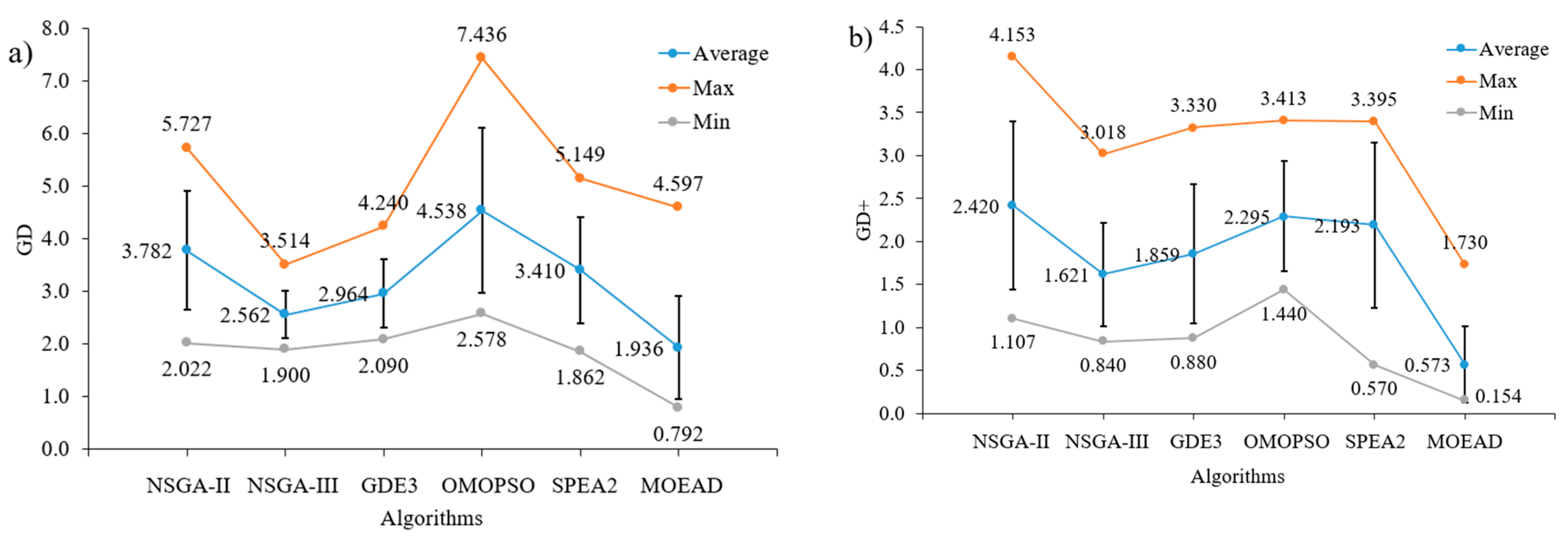
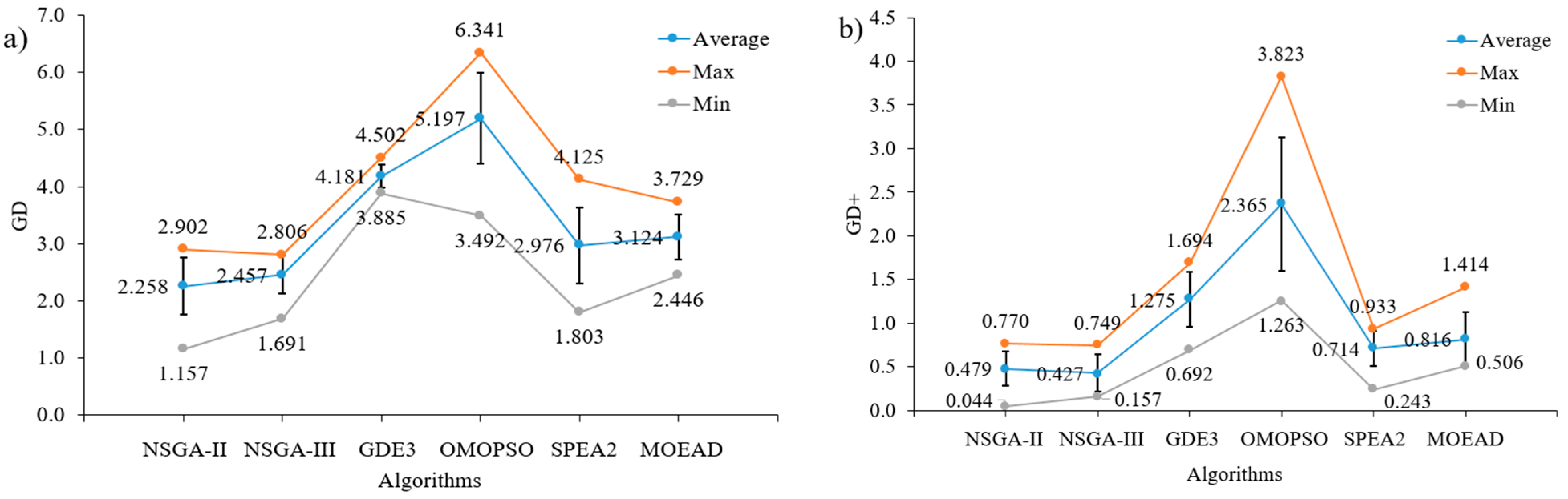
Figure 5 presents the calculated values of GD, GD+, IGD+, and HV of MOO algorithms of the 10-bar truss. Note that GD, GD+, and IGD+ were determined by using the above approximate Pareto-front while HV was computed using the reference point with the coordinate values of the maximum objective functions in all of the obtained optimal results plus 1.1. As can be seen in Figure 5a–d, MOEA/D had the best performance since it achieved the smallest values of GD, GD+, and IGD+ and the greatest value of HV. In detail, the average values of GD, GD+, IGD+, and HV of MOEA/D were 1.936, 0.573, 2.466, and 70,097.2, respectively. In the five remaining MOO algorithms, NSGA-III had the smallest values of GD and GD+, which were equal to 2.562 and 1.621, respectively. However, GDE3 yielded the smallest value of the average IGD+ with 4.567 and the greatest value of the average HV with 67369.3. However, in general, the performance of NSGA-II, NSGA-III, GDE3, OMOPSO, and SPEA2 was quite similar in terms of the GD, GD+, IGD+, and HV indicators.

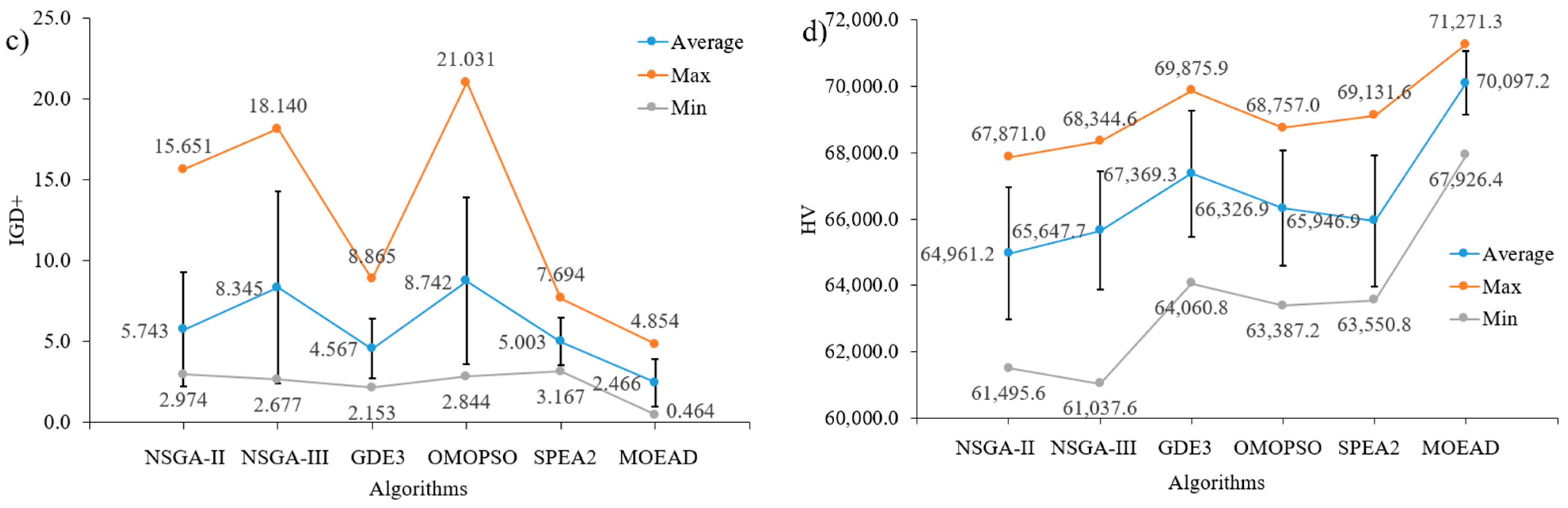
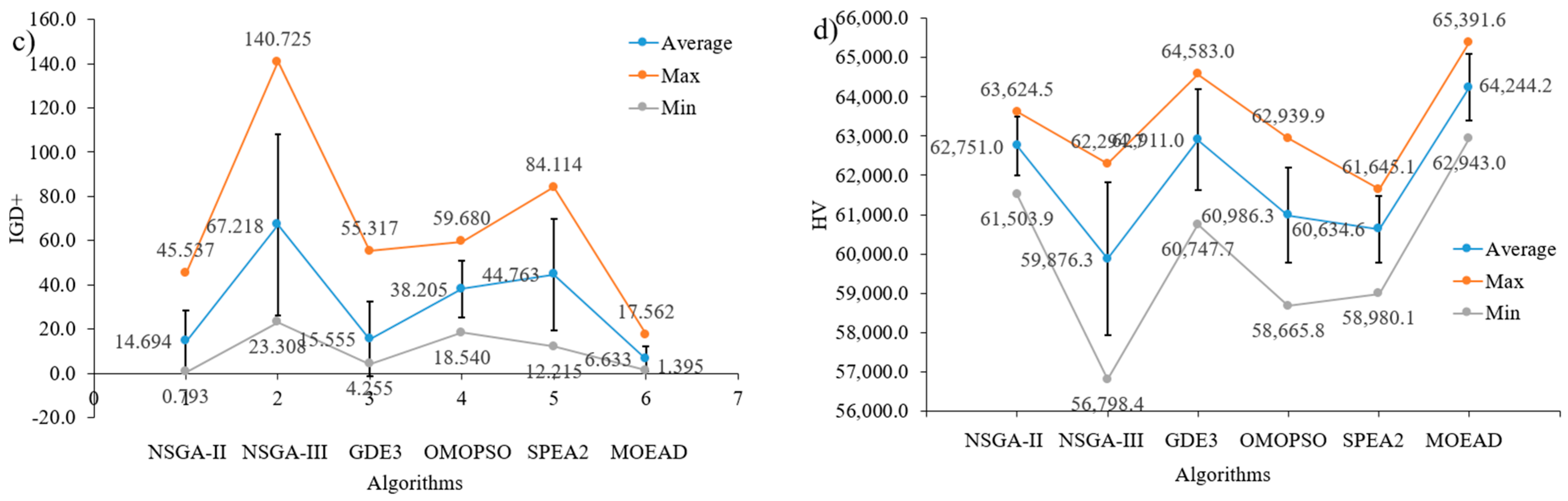
To evaluate the solution spread of the MOO algorithms, Figure 6 presents the minimum values of two considered objectives. As can be seen in Figure 6a, if the minimization of the total structural weight is important, NSGA-II achieved the smallest result of 2004.1 (kg). However, the stability of MOEA/D was the best with the smallest value of 2087.5 (kg) of runs. At the same time, the dispersion of the MOEA/D results was also minimal among the MOO algorithms. In Figure 6b, when the minimization of the second objective function was important, MOEA/D yielded the best optimal result of 20.028 (mm). This algorithm also had the best stability with the smallest average value of 20.285 (mm). The performance of the five remaining algorithms seems similar. 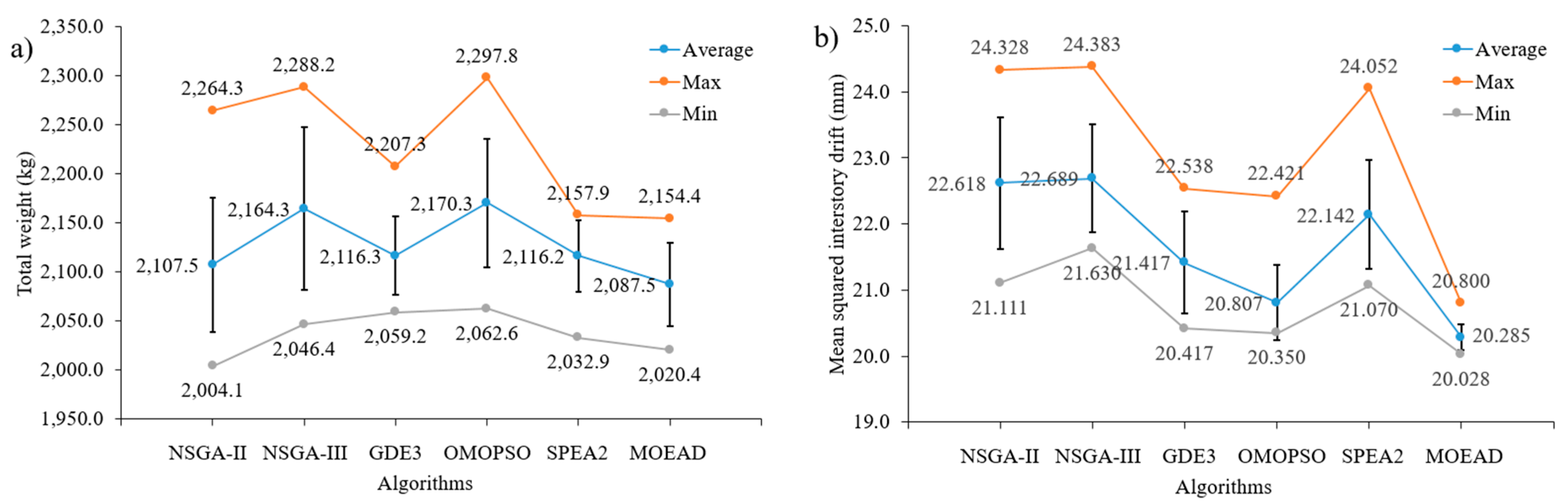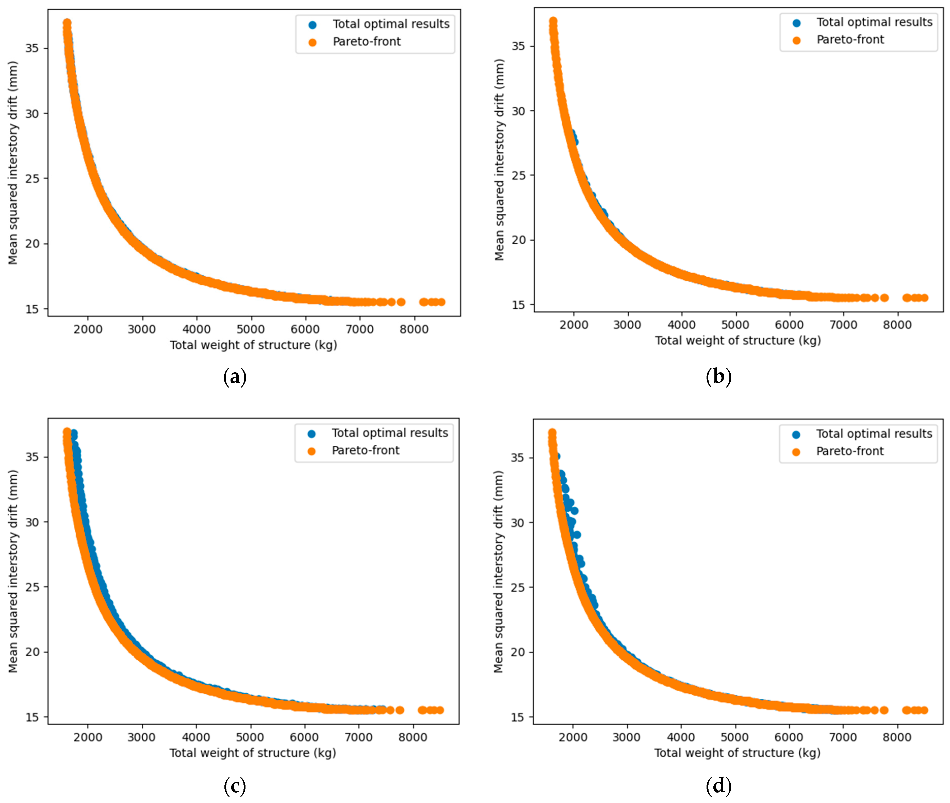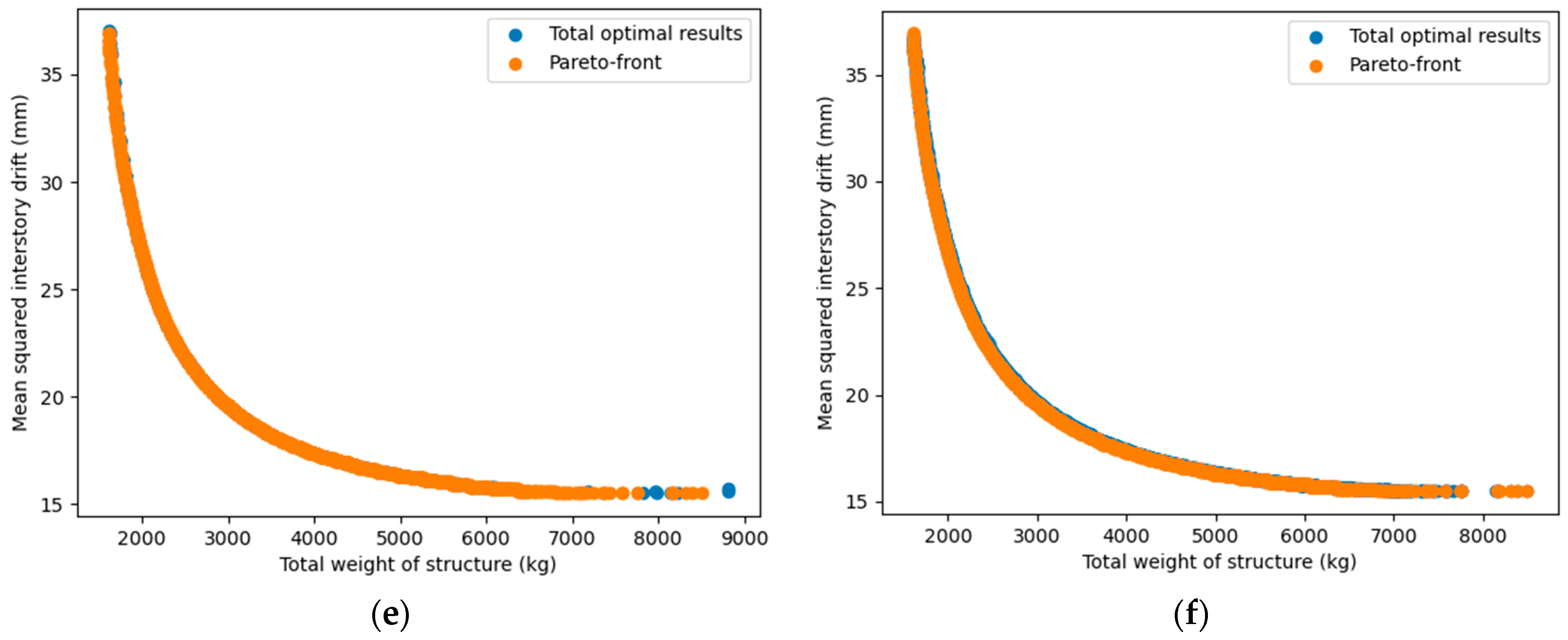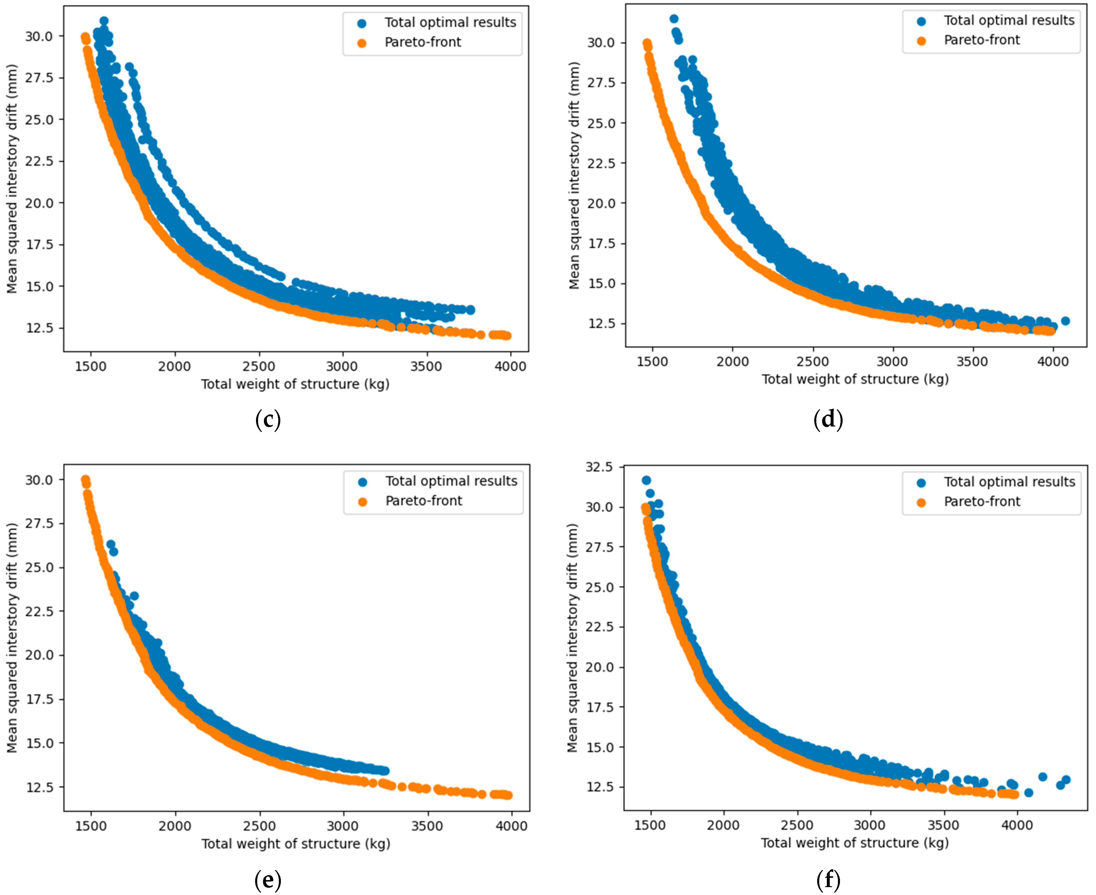For more visualization, Figure 7 presents the Pareto-front curve with all optimal points obtained using each algorithm. Obviously, MOEA/D had a better spread compared to the other algorithms.

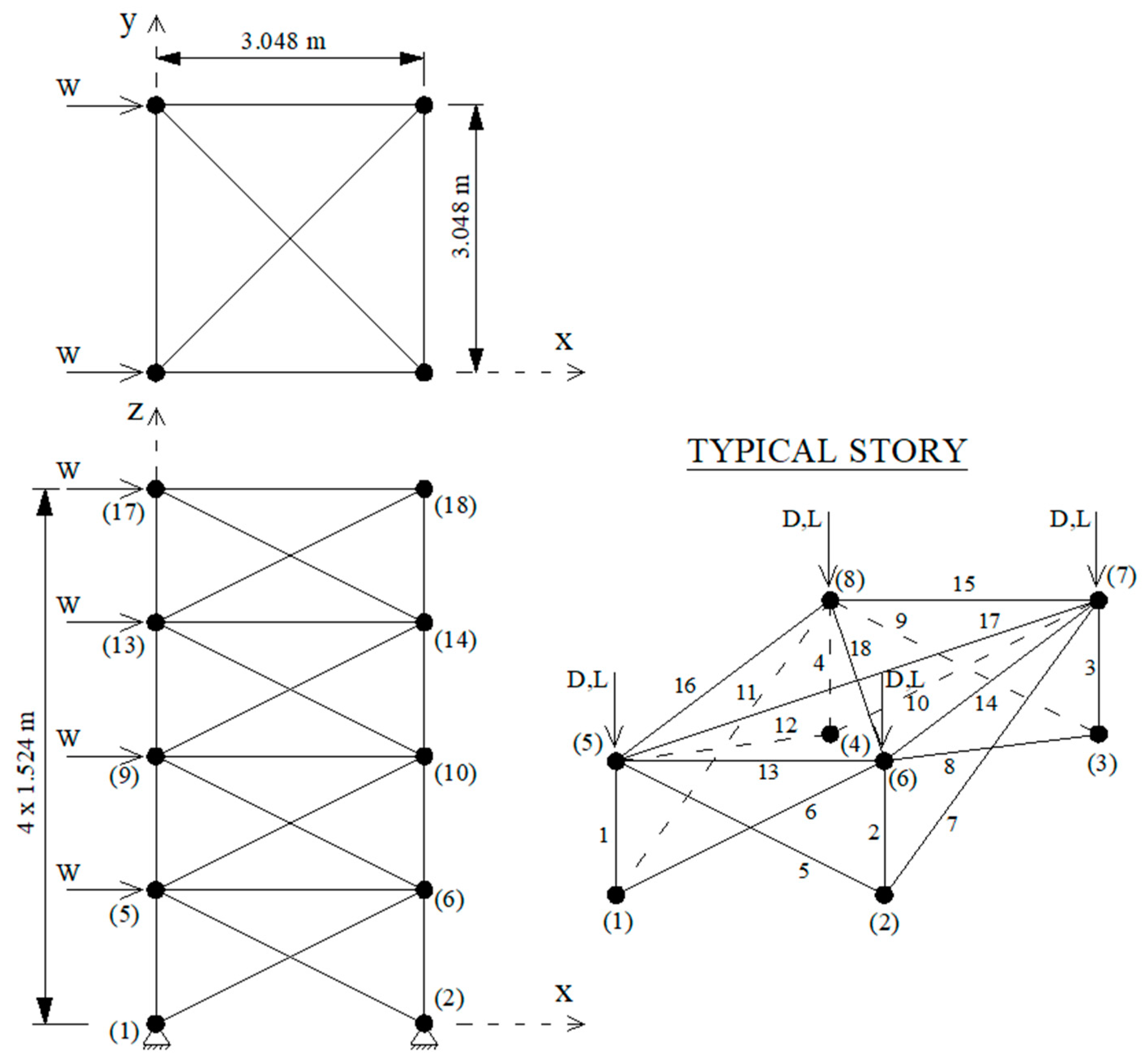
4.2. Spatial 72-Bar Truss

The second example was a spatial 72-bar truss with the layout and geometric presented in Figure 8. The structural elements were classified into 16 cross-sectional groups including (1) A₁-A₄; (2) A₅-A₁₂; (3) A₁₃-A₁₆; (4) A₁₇-A₁₈; (5) A₁₉-A₂₂; (6) A₂₃-A₃₀; (7) A₃₁-A₃₄; (8) A₃₅-A₃₆; (9) A₃₇-A₄₀; (10) A₄₁-A₄₈; (11) A₄₉-A₅₂; (12) A₅₃-A₅₄; (13) A₅₅-A₅₈; (14) A₅₉-A₆₆; (15) A₆₇-A₇₀; (16) A₇₁-A₇₂. The dead load (D), live load (L), and wind load (W) were equal to 100, 50, and 40 (kN), respectively. The information on the load combinations considered was the same as in the first case study. 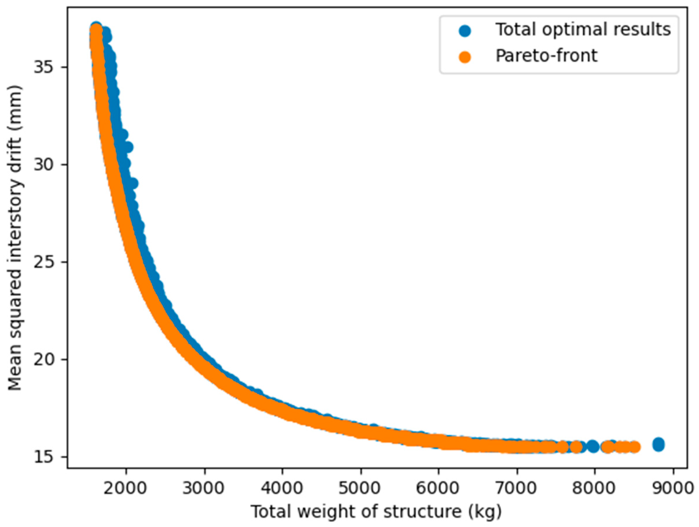The first objective was the total weight of the structure and the second objective was $F_2\left(\mathrm{X}\right)=\sqrt{x_5^2+x_9^2+x_{13}^2+x_{17}^2}$, where x₅, x₉, x₁₃, and x₁₇ are the horizontal displacements of nodes 3, 9, 13, and 17, respectively. The approximate Pareto-front and all optimal solutions found in this case study are presented in Figure 9.

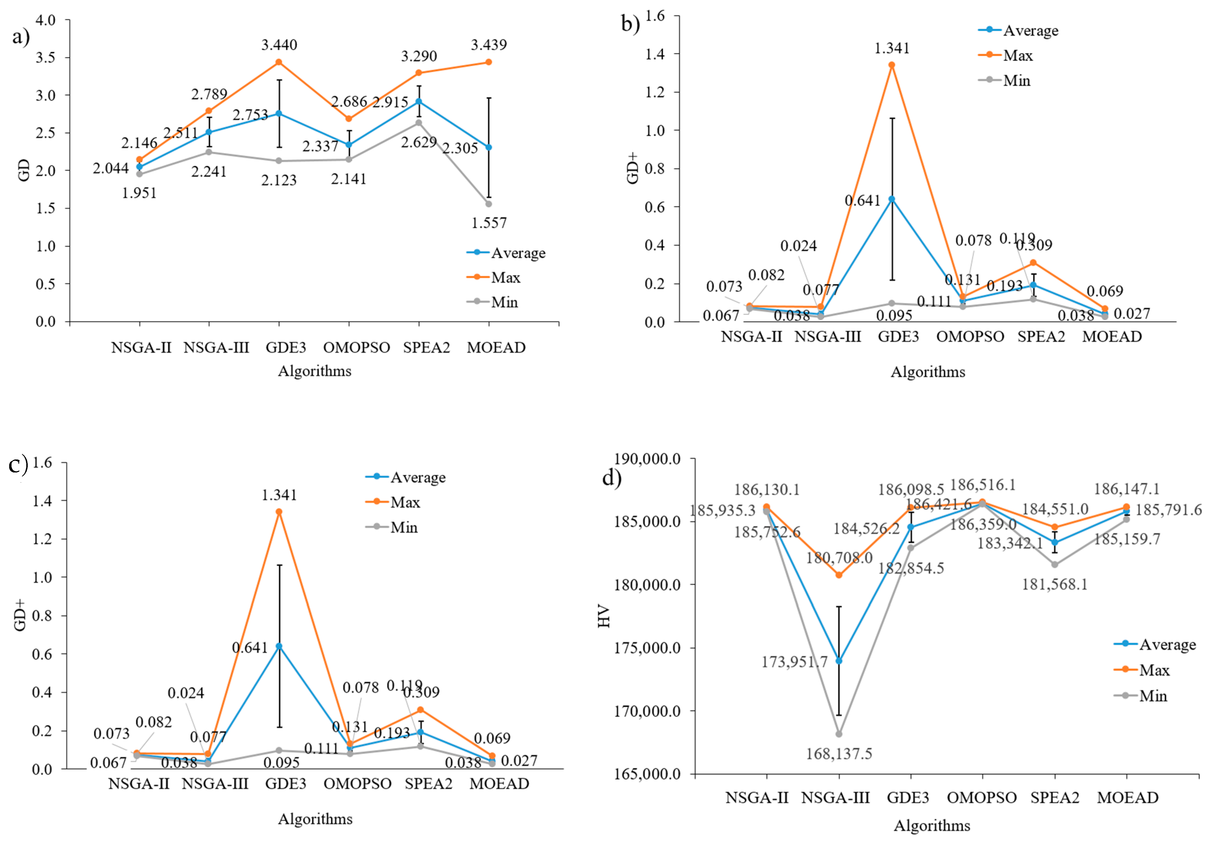
The calculated values of GD, GD+, IGD+, and HV of the MOO algorithms are presented in Figure 10. As can be seen in Figure 10a, MOEA/D had the smallest value of GD with 1.557. However, NSGA-II seemed to have a better performance among the algorithms with the smallest average values of 2.044 and dispersion of the results. However, regarding GD+ and IGD+, MOEA/D yielded the best results among the algorithms in terms of both the value and stability. NSGA-II and OMOPSO ranked second, while GDE3 and NSGA-III were not good with GD+ and IGD+, respectively. Regarding the HV indicator, OMOPSO was the best, but was only slightly better than NSGA-II and MOEA/D. NSGA-III was the worst with the smallest value of HV and poor stability.

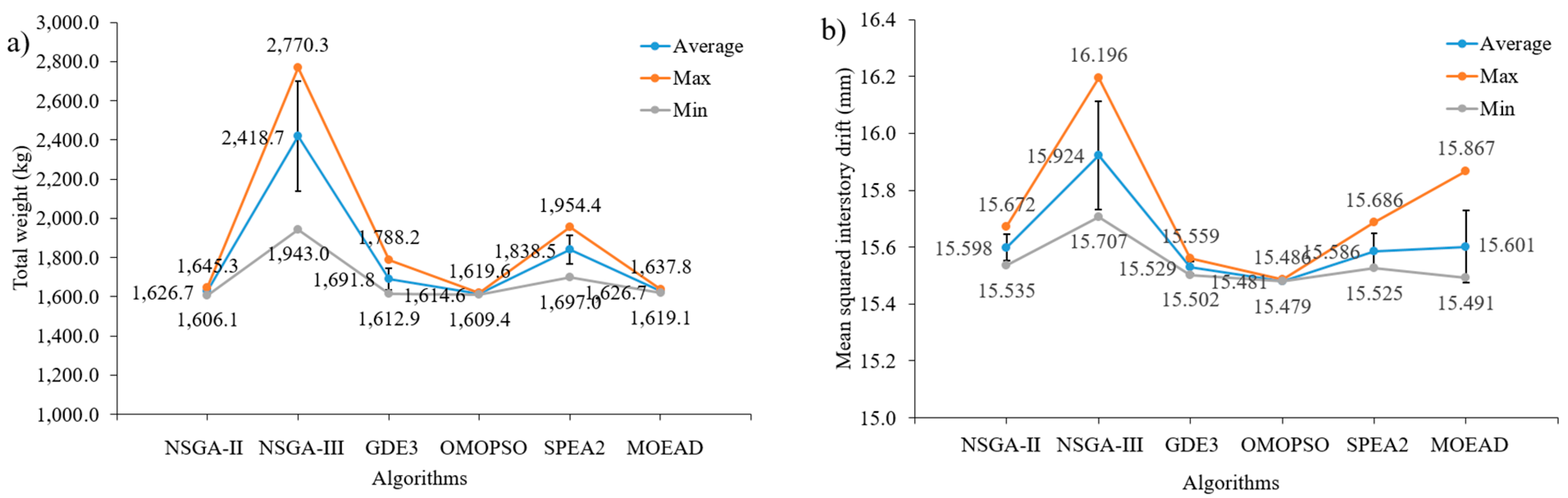
Figure 11 presents the minimum values of two considered objectives to evaluate the solution spread of the algorithms. As can be seen in Figure 11a, if the minimization of the total structural weight was important, NSGA-II achieved the smallest result of 1606.1 (kg) and the second was OMOPSO with 1609.4 (kg). However, the stability of OMOPSO was the best with the smallest value of 1614.6 (kg) of runs, and was just slightly better than that of NSGA-II and MOEA/D. In Figure 11b, when the minimization of the second objective function was important, OMOPSO found the best optimal result of 15.479 (mm). The performance of NSGA-III was the worst in both case studies. Figure 12 presents the Pareto-front curve with all optimal points obtained using each algorithm.

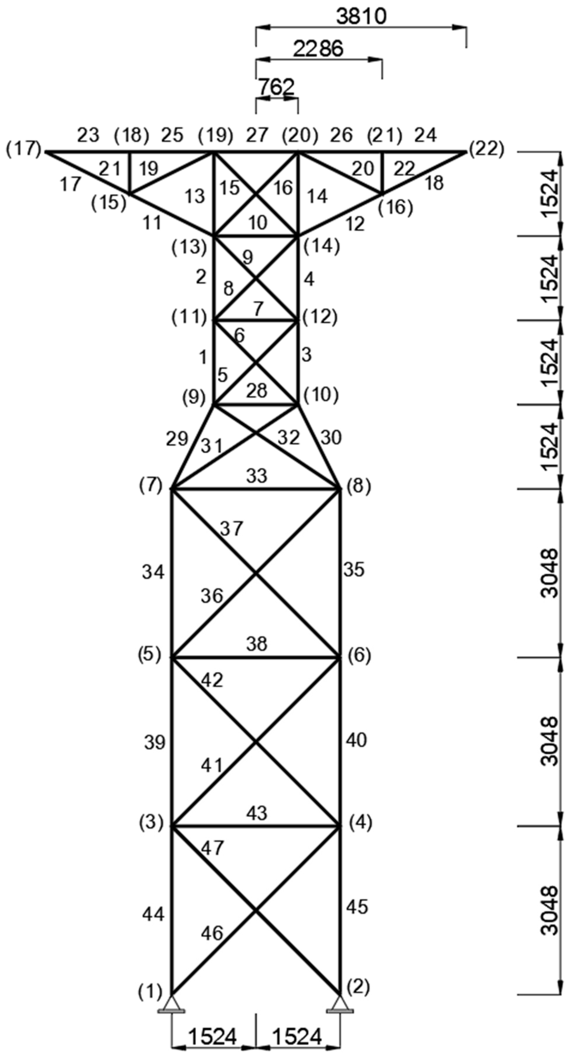
4.3. Planar 47-Bar Power Line Truss

The third example was a 47-bar power line truss with the layout and geometric presented in Figure 13. Cross-sectional areas of member groups were divided into 27 groups such as (1) A₁-A₃; (2) A₂-A₄; (3) A₅-A₆; (4) A₇; (5) A₈-A₉; (6) A₁₀; (7) A₁₁-A₁₂; (8) A₁₃-A₁₄; (9) A₁₅-A₁₆; (10) A₁₇-A₁₈; (11) A₁₉-A₂₀; (12) A₂₁-A₂₂; (13) A₂₃-A₂₄; (14) A₂₅-A₂₆; (15) A₂₇; (16) A₂₈; (17) A₂₉-A₃₀; (18) A₃₁-A₃₂; (19) A₃₃; (20) A₃₄-A₃₅; (21) A₃₆-A₃₇; (22) A₃₈; (23) A₃₉-A₄₀; (24) A₄₁-A₄₂; (25) A₄₃; (26) A₄₄-A₄₅; (27) A₄₆-A₄₇. The dead and live loads were simulated as the vertical point loads at all nodes and were equal to 70 (kN) and 50 (kN), respectively. The wind load of 30 (kN) was according to the X-axis at nodes 17 and 22. The information on load combinations considered was the same as in the above case studies. The first objective was the total weight of the structure and the second objective was $F_2\left(\mathrm{X}\right)=\sqrt{x_3^2+x_5^2+x_7^2+x_9^2+x_{11}^2+x_{13}^2{+}_{15}^2+x_{17}^2}$, where x_i is the horizontal displacements of the node ith. 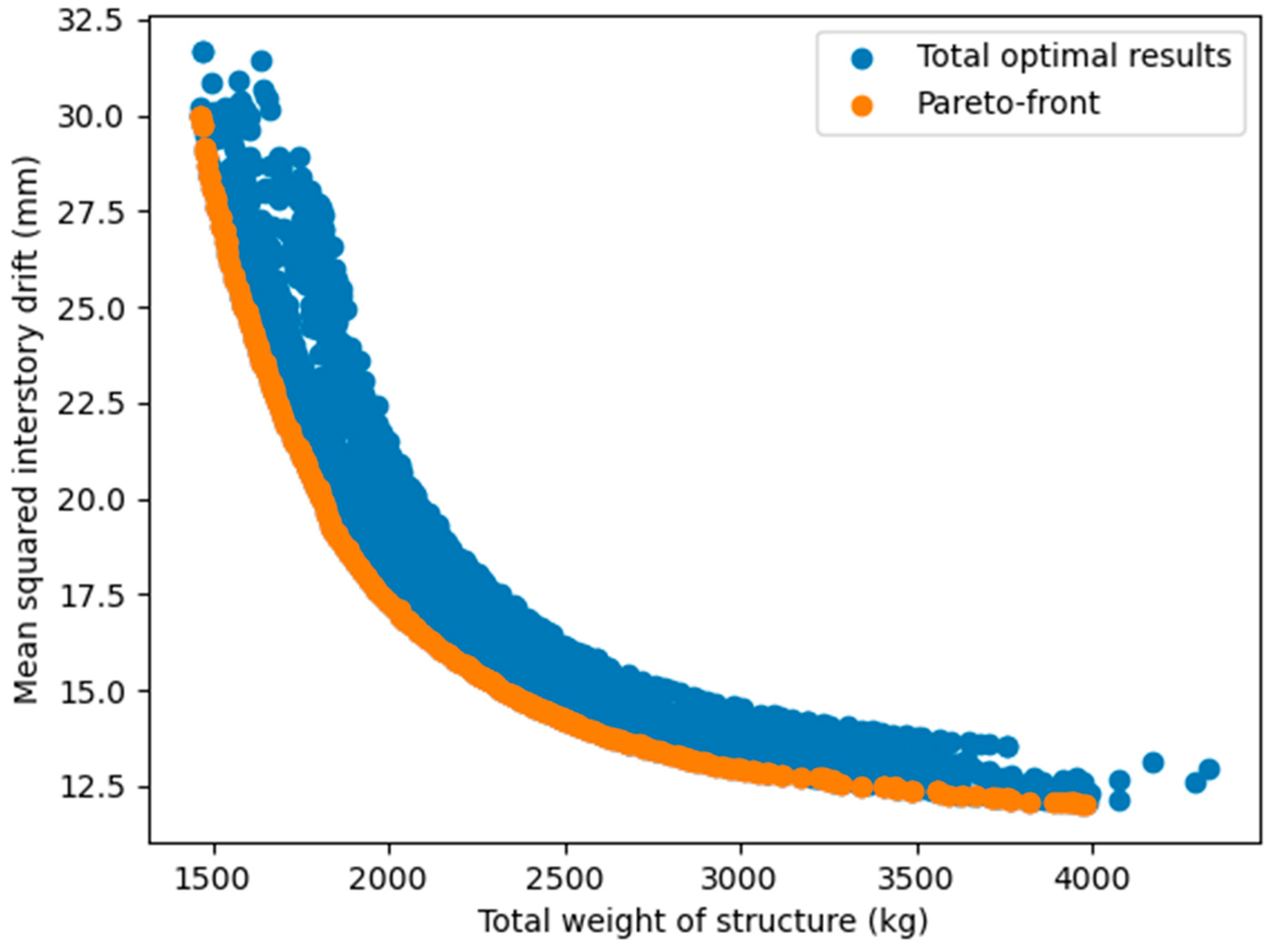Figure 14 illustrates the approximate Pareto-front and all optimal solutions found in this case study.

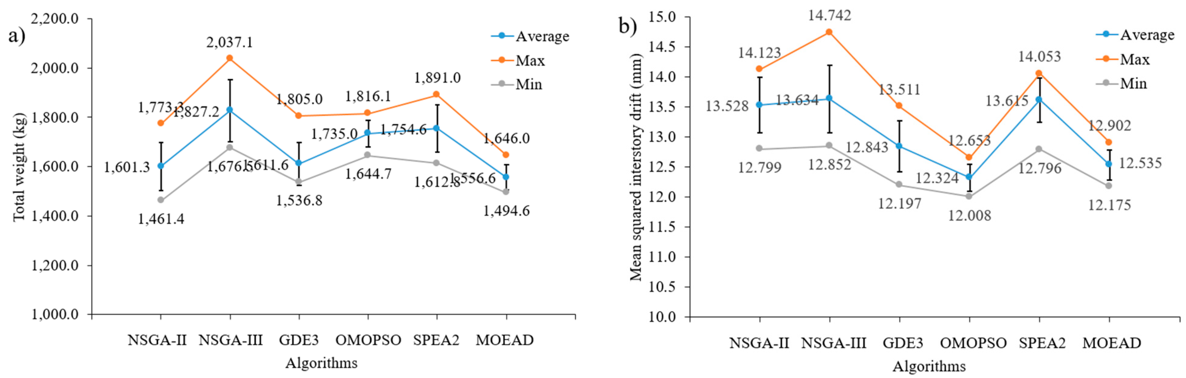
Figure 15 shows the GD, GD+, IGD+, and HV values of the MOO algorithms. As can be seen in Figure 15a,b, NSGA-II and NSGA-III had the smallest values of GD and GD+. The second was SPEA2 and MOEA/D, and the worst was OMOPSO. Regarding the IGD+ and HV indicators, MOEA/D yielded better results among the considered algorithms while NSGA-III was the worst. GDE3 ranked second with slightly better than NSGA-II. Figure 16 presents the minimum values of two considered objectives. If the minimization of the total structural weight is important, NSGA-II achieved the smallest result of 1461.4 (kg), and the second was MOEA/D with 1494.6 (kg). However, the stability of MOEA/D was the best with the smallest average value of 1556.6 (kg) of runs, but was just slightly better than that of NSGA-II and GDE3. In Figure 16b, when the minimization of the second objective function was important, OMOPSO found the best optimal result of 12.008 (mm). Once again, the performance of NSGA-III was the worst in both case studies. Figure 17 presents the Pareto-front curve with all optimal points obtained using each algorithm.

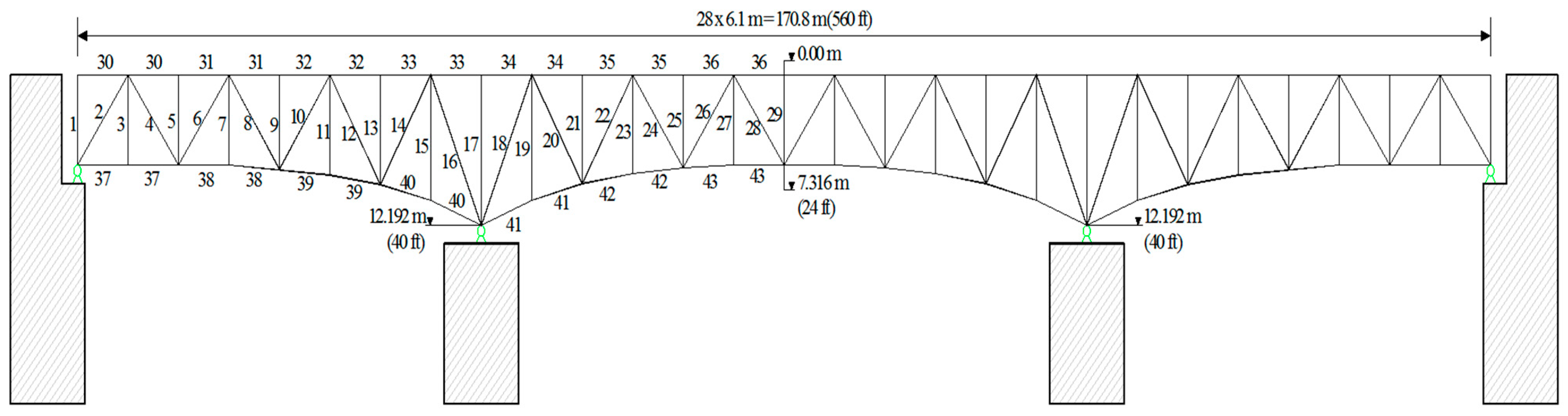
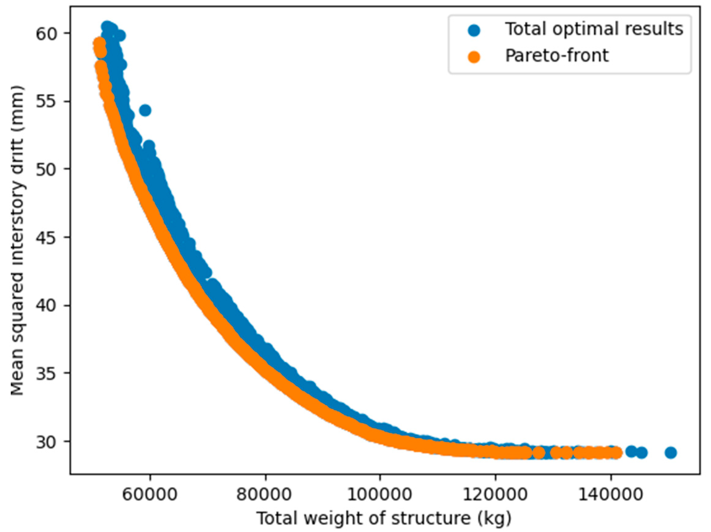
4.4. 113-Bar Plane Truss Bridge

The last example was a 113-member plane truss bridge with 43 independent groups, as presented in Figure 18. Cross-sectional areas of the member groups were considered as design variables of the optimization problem and were in the range [3870.96, 22,580.6] (mm²). The strength and serviceability load combinations considered were (1.25D + 1.75L) and (1.0D + 1.0L), respectively. The dead and live loads were simulated as the point loads at every truss joint on the upper chord equaling 100 (kN) and 50 (kN), respectively. The first objective was the total weight of the structure and the second objective was $F_2\left(\mathrm{X}\right)=\sqrt{y_1^2+y_2^2}$, where y₁ and y₂ are the vertical displacements of the middle points of the side and main spans of the bridge, respectively. The constraints relating to the serviceability load combination were to limit the vertical displacement of the middle points to be greater than 43.1 (mm). 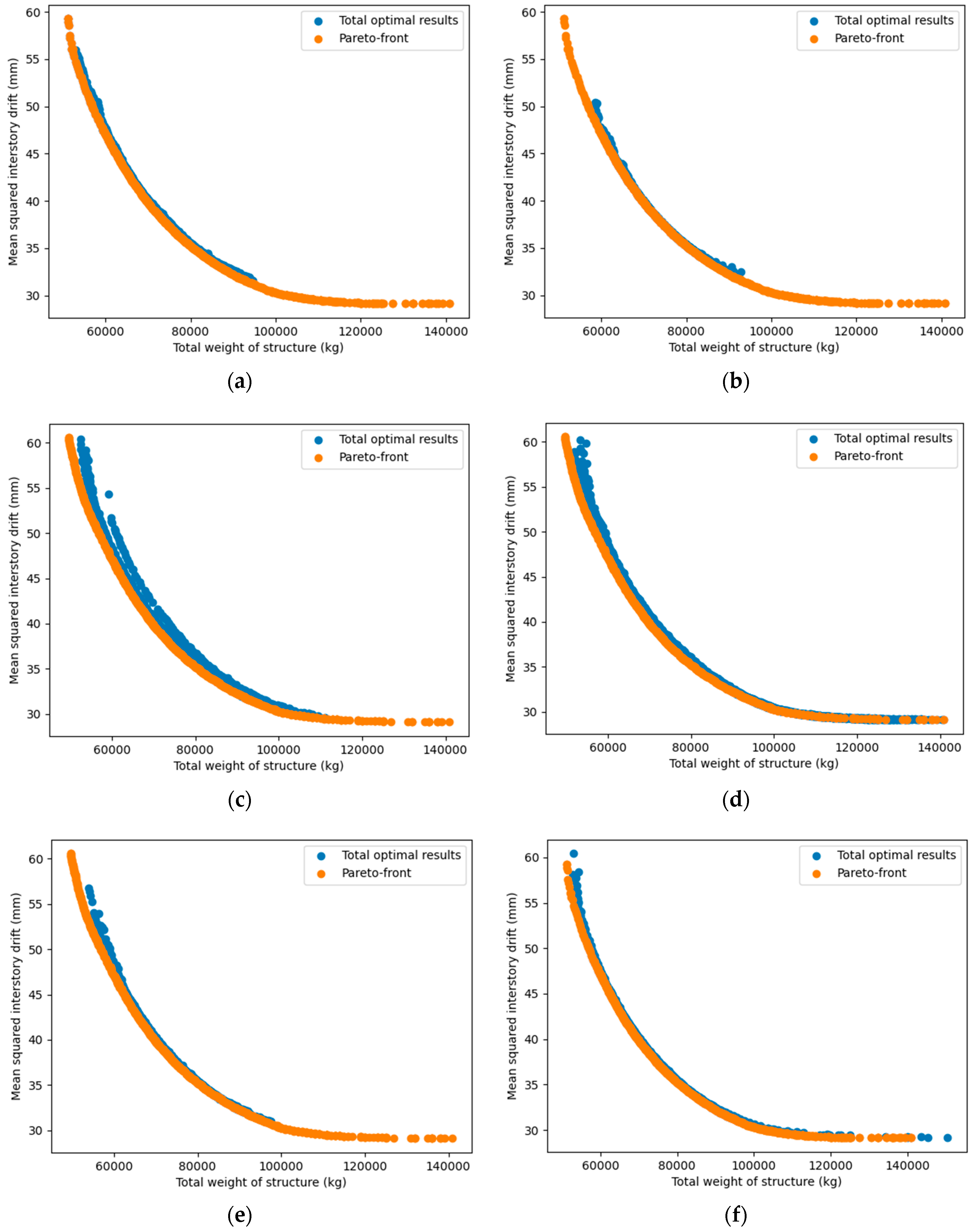Figure 19 presents the approximate Pareto-front and all of the optimal solutions found.

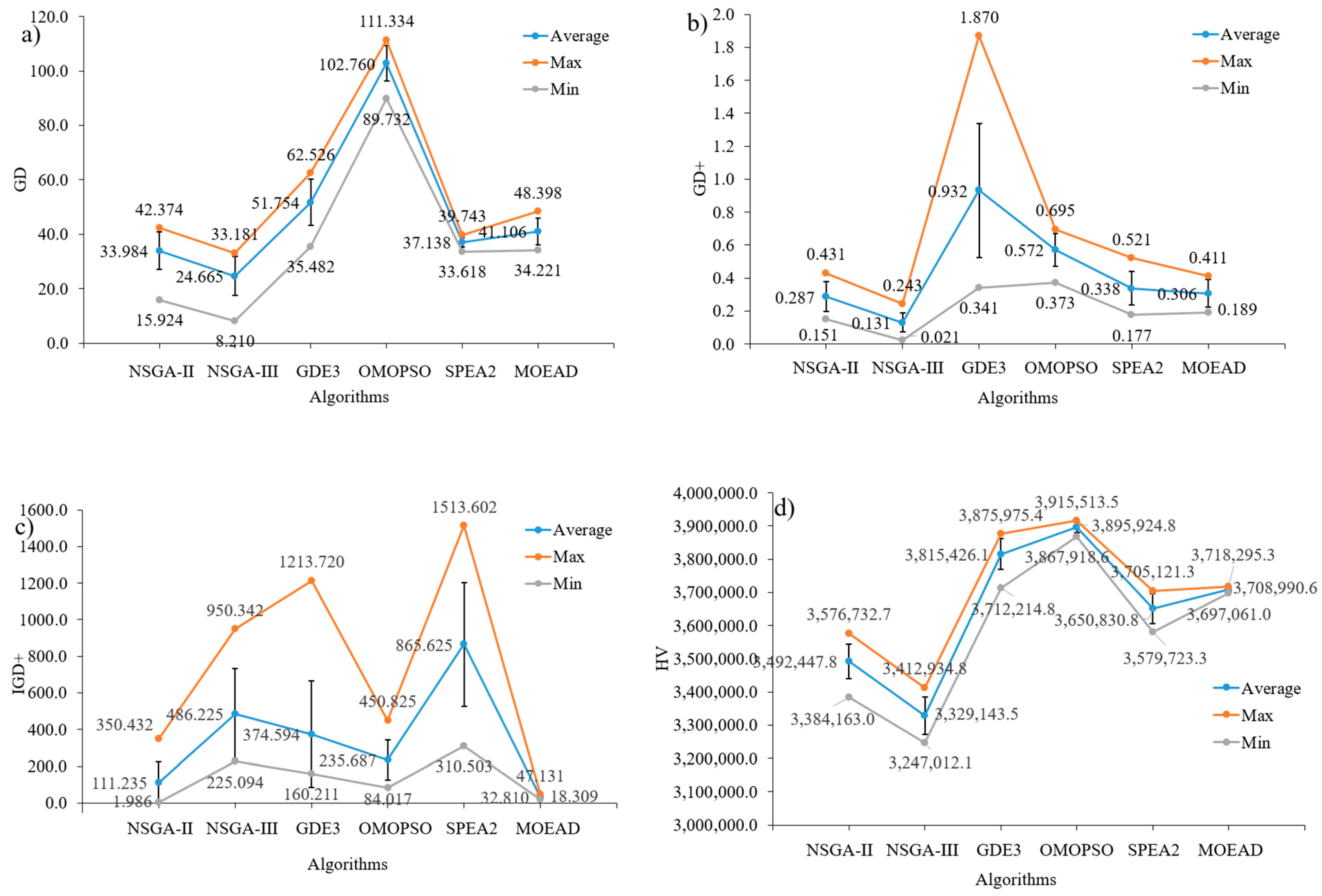
Figure 20 illustrates the GD, GD+, IGD+, and HV values of the MOO algorithms. As can be seen in Figure 20a,b, NSGA-III and NSGA-II had the smallest values of GD and GD+. The second was SPEA2 and MOEA/D, and the worst was OMOPSO for GD and GDE3 for GD+. Regarding IGD+, NSGA-II and MOEA/D had better performance than the other considered algorithms. SPEA2 and GDE3 were the worst. However, regarding the HV indicator, the best performance was OMOPSO and GDE3, while the worst was NSGA-III. 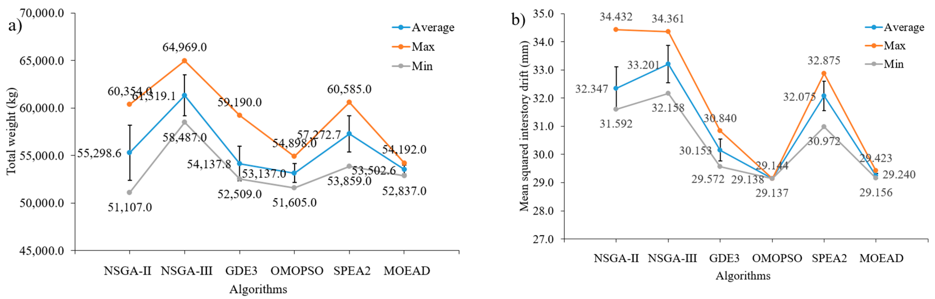The minimum values of the two considered objectives are presented in Figure 21. Once again, NSGA-II achieved the smallest result of 51,107.0 (kg) when the minimization of the total structural weight was important. The second was OMOPSO with 51,605.0 (kg). In Figure 21b, when the minimization of the second objective function was important, OMOPSO found the best optimal result of 29.137 (mm), which was slightly better than the result of MOEA/D with 29.156 (mm). The performance of NSGA-III was the worst in both case studies. Figure 22 presents the Pareto-front curve with all optimal points obtained using each algorithm.

4.5. Discussions

The above numerical results provided us with useful information on the multi-objective optimization of steel frames using direct analysis. As presented in Figure 4, Figure 9, Figure 14 and Figure 19, the relationship between two objectives (structural weight and inter-story drift or lateral displacement) was nonlinear and inversely proportional to each other. This was completely consistent with our forecast, and also showed that the use of a multi-objective problem, in this case, was necessary and reasonable. Based on the multi-objective optimization problem built, all six considered MOO algorithms showed a high efficiency since they successfully searched for feasible optimal solutions in all independent runs. Generally, the numerical results proved that no algorithm outperformed the others. However, if we consider the overall performance in all four case studies, NSGA-II and MOEA/D were somewhat more effective in both searching the Pareto and anchor points. Compared to MOEA/D, NSGA-II seemed to find better Pareto solutions, but its stability and optimal solution spread were worse. Among the remaining algorithms, NSGA-III effectively yielded Pareto points, but was less efficient in finding anchor points. OMOPSO also had a good performance, especially in finding the anchor points, but was less stable than MOEA/D. GDE3 and SPEA2 were only average in all case studies.

5. Concluding Remarks

The current work successfully developed the multi-objective optimization of steel trusses using direct analysis. Two conflict objectives were minimized including the total weight and the inter-story drift or displacements in the structure. Nonlinear inelastic analysis and nonlinear elastic analysis were used to evaluate the constraints relating to the strength and serviceability load combinations, respectively. Six well-known metaheuristic algorithms such as NSGA-II, NSGA-III, GDE3, OMOPSO, SPEA2, and MOEA/D were employed to solve the developed MOO problems. Four truss structures were studied including a planar 10-bar truss, a spatial 72-bar truss, a planar 47-bar powerline truss, and a planar 113-bar truss bridge. The numerical results proved that the relationship between the two objectives was nonlinear and inversely proportional to each other. Generally, all six algorithms successfully found feasible optimal solutions and no algorithm outperformed the others. In detail, NSGA-II and MOEA/D were better at both searching for the Pareto and anchor points. MOEA/D was more stable and had a better solution spread. OMOPSO was also good at solution spread, but its stability was worse than that of MOEA/D. NSGA-III seemed to be less efficient in searching for anchor points, although it could effectively yield Pareto points. A future extension of this study is to develop a novel combination of metaheuristic algorithms for MOO problems to enhance the advantages of the considered algorithms. This is currently under study by the authors.