Article

Structural Landmark Salience Computation in Compact Urban Districts with 3D Node-Landmark Grid Analysis Model: A Case Study on Two Sample Districts in Changsha, China

1
Department of Landscape Architecture, Central South University of Forestry and Technology, Changsha 410004, China
2
Hunan Big Data Engineering Technology Research Center of Natural Protected Areas Landscape Resources, Changsha 410004, China
*
Author to whom correspondence should be addressed.
Buildings 2023, 13(4), 1024; https://doi.org/10.3390/buildings13041024
Submission received: 24 February 2023 / Revised: 4 April 2023 / Accepted: 11 April 2023 / Published: 13 April 2023

Abstract

:
Mastering the relationship between urban landmarks and urban space morphology in urban planning, landscape planning, and architectural design helps maintain the intelligibility of compact urban districts. The objective of the present study was to numerically determine the structural salience of various landmarks in an urban environment and use it to interpret the intelligibility of the city. Combining the measurement method of 3D visibility and the related principles of space syntax, this study develops a new 3D Node–Landmark Grid Analysis Model (3D NL GAM) for structural salience computation of urban landmarks. In this study, a numerical approach is used to construct a 3D simulation model. Firstly, the visibility of each decision node to landmarks in an urban environment, using a 3D digital model, is measured using the 3D isovist component of Rhinoceros and Grasshopper software. Secondly, links among wayfinding decision nodes and landmarks are established to form a 3D NL GAM. The normalized angular integration of decision nodes and the normalized angular choice of landmarks are computed using the principle of space syntax. Thirdly, the structural salience of landmarks is determined with a function of landmark visibility, spatial properties of landmarks, and wayfinding decision nodes. Finally, a case study was carried out by using a 3D NL GAM to analyze three types of urban areas located in Changsha. The results indicated that large-scale natural landscapes have a higher structural salience among the types of landmarks. The structural salience of architectural landmarks in the combined spatial form of combining tall and low building groups has a clear advantage over the form dominated by high-rise building groups. Raising the height of landmark buildings can modify the structure of the grid analysis model and improve the people aggregation of urban space. The 3D NL GAM can quantify the spatial properties and landmark structural salience of a city and can effectively assist in the evaluation of the intelligibility of built or future urban environments.

Graphical Abstract

1. Introduction

Compact cities are an important means of sustainable development and are conducive to the intensification of urban resources, but they also present higher requirements for urban planning, landscape planning, and architectural design [1,2,3]. UN-Habitat advocates moderately compact and high-density cities, and suggests that the population density of future urban planning should be greater than 150 people per hectare [4]. This has led to higher population densities, mixed-function land use, more centralized public facilities, compact residential built communities within a given urban area, and the development of vertical space. “Intelligibility” plays a crucial role in the quality of urban space [5].
However, high density and high-rise clusters in compact cities tend to block views in urban spaces, which affects the permeability of urban spaces and undermines urban intelligibility. Therefore, intelligibility in urban environments has become an important topic in urban design for compact cities. In order to ensure the quality of urban space and enhance urban intelligibility, urban designers need to think about the following questions: (1) how to obtain comfortable perception density in urban street space [6,7,8], (2) ensuring the synergy of landmarks, (3) how to garner the necessary landscape resources, (4) the synergy between specific location and the overall environment [9,10], and (5) other urban image elements in relation to urban residents’ activities. Among them, where clarifying the structural relationship of landmarks in compact urban areas, accurately describing the structural salience of landmarks in a compact urban environment is a key issue for enhancing urban intelligibility.
Urban intelligibility is the original goal of urban imagery in terms of how people orient themselves and navigate the city [5,11]. People’s actions are governed by their visual perception and influenced by the characteristics of urban imagery. In essence, urban imagery describes the structural salience of the city’s elements in relation to each other [9,12]. The integration of the five elements of urban imagery reflects the behavior of people moving in the city, i.e., for a person moving in an urban area, this is the process of perceiving and acting in this area, with boundaries determining the scope of analysis, paths as channels, nodes as decision points for action, and landmarks as references. Therefore, the structural salience of landmarks is based on the integration of nodes, paths, areas, and boundary forms, expressing the role of landmarks in the spatial structure of urban areas and their relationship with other elements [13].
The structural salience of landmarks has substantial implications for wayfinding and navigation in cities [13,14,15,16]. Caduff et al. generated landmark route navigation using a landmark saliency-weighted path algorithm and compared landmark routes with shortest-distance routes, which demonstrates the advantage of landmark routes for navigating route selection in most cases [17,18]. Simulation analysis agent-based modeling has shown [19] that the route selection model containing landmarks provides directional guidance and environmental characteristic variability, thus expressing more urban information. That is, the urban information conveyed by landmarks is related to the visibility of landmarks, and the analysis of landmarks in urban areas should consider not only neighboring but also distant landmarks. In terms of the location relationship between landmarks and pathfinders, landmarks are usually classified into global and local landmarks [15,20]. Global landmarks refer to landmarks that can be seen from a large distance, and a global reference system, such as the efficacy of a compass in landmark routes. Local landmarks can only be seen from a small distance; they are only visible in a limited area and only from a specific method [15,20]. Studies have shown that both local and global landmarks are used for decision making [15,20,21,22].
However, there has been a lack of quantitative characterization metrics and scientific analytical methods to describe the structural salience of landmarks in urban spaces [23]. In terms of landmarks and human wayfinding needs, landmarks are defined as “geographic objects that constitute human mental representations of space” [24], and landmark representations are the result of the local integration of visual, motor, and spatial information [25]. Klippel and Winter determined the structural salience of landmarks from the semantic expression of the positional relationship between landmarks and navigation routes. This is a kind of qualitative research method focused on navigation route arrangement [26], where it is difficult to form a difference comparison for the structural salience of landmarks. Winter also proposed an extension of the advance visibility assumption, in which landmarks can be identified early along the roadway with valid landmark structural saliency [27], but does not provide a measure of visibility in complex 3D urban environments and miscellaneous road grids. Therefore, the structural salience of landmarks in urban environments is a unique property of the cognitive and physiological trilateral relationship between the landmark feature itself, its surroundings, and the observer’s perspective [11,14,28].
Space syntax theory provides methods for measuring spatial node accessibility and directional guidance in cities [29]. Claramunt and Winter adopted the method of mathematical graph theory and space syntax to analyze the saliency of regions, boundaries, streets, and nodes and formed a structural model of urban element recognition [12,30]. It has been shown that the principles of space syntax are suitable for the structural description of urban spatial forms, and quantitative analytical results can be obtained. However, this analytical approach does not deal with distant landmarks on the one hand, nor does it consider the impact of the visibility of nearby landmarks on the urban structure model. Therefore, based on the two-dimensional limitation of urban grids, space syntax cannot adequately describe landmarks [31]. Enhancements based on 3D isovist generation techniques have promoted the development of spatial syntactic analysis toward 3D spatial analysis. These have been realized in spatial analyses regarding the measurement of urban spatial openness [32], the spatial morphological characteristics [33], as well as visual permeability measurements [34]. Detailed representations of spatial visibilities have been implemented in these studies, but they have not been synchronously implemented for the visibility of a particular object.
The above literature gives an important insight that if a 2D grid analysis model for an urban network can be developed into a 3D grid analysis model, then the objective of accurately quantifying the structural saliency of landmarks is possible. Two conditions must be satisfied to achieve this objective. First, visibility measurements of urban landmarks are implemented for all the wayfinding decision nodes in a 3D environment. Second, the spatial properties of landmark locations and the spatial properties of wayfinding decision nodes are implemented for directional guidance and spatial accessibility. With the improvement of computer hardware and software technology, the current measurement technology for both 3D digital models of cities and visibility data of spatial places has been significantly improved [35,36]. Meanwhile, there is a mature research paradigm for analyzing the relationship between urban spaces using space syntax [37,38]. In order to achieve these two fundamental conditions, the next section is devoted to a literature review on the construction of a grid analysis model based on space syntax, and the presentation of a 3D isovist.
Based on the literature and analysis, this study develops a 3D Node–Landmark Grid Analysis Model (3D NL GAM) to incorporate the 3D visibility data of landmarks into the spatial syntactic analysis model. In the context of compact cities, this paper aimed to clarify the integrated relationship between landmarks and textural features in urban areas. In particular, the relationship between natural landscape resources, street grids, the combined forms of different architectural groups, and the landmark’s own form was examined and used to guide the evaluation of urban intelligibility and the urban design.

2. Literature Review

2.1. Grid Analysis Model Based on the Principle of Space Syntax

Space syntax is a scientific reconstruction of how people interact with their environment. This helps to understand the relationship between humans and their environment by creating a model that connects real spaces with human cognitive structures through logical spaces (employing signs, symbols and representations to create schematized multidimensional spaces) [39]. After more than 50 years of development, space syntax has become a paradigm for spatial research, and is linked to other disciplines or research fields [40]. Using the principles of space syntax, the city is understood as a network formed by space, thus establishing a link between human behavior and network science in the urban environment [41,42]. The analytical method of space syntax can be used to analyze the urban street networks, functional layouts, data on urban points of interest, as well as the structure of urban centers and other mobile features of human agglomeration and dispersion in the urban environment [43,44,45,46].
Traditional grid analysis models for space syntax include convex map analysis [47], axial map analysis [48], and Visibility Graph Analysis (VGA) [49,50]. An urban network is used to abstractly express the location, connectivity relationships, and the structure of the city’s nodal spaces in a region-wide system, as well as to form a corresponding structural form with various types of analytical models [51,52,53]. The approach to grid construction is consistent with the principles of mathematical graph theory, i.e., a grid graph is composed of nodes and lines, where nodes correspond to the vertices of the graph, in mathematical graph theory, and lines correspond to the edges of the graph [30]. Thus, there are two core tasks for constructing an analytical model:
  • Investigating as to how the logical space expresses the real space of the city;
  • Establishing links between spatial nodes.
Traditionally, there are three ways to construct a grid. The first way is to consider streets as spatial nodes, with axes acting as the logical space of streets and intersections between the streets acting as connecting edges, which is used to calculate the motion properties of street space in the form of an axial analysis map [29]. The second way treats street intersections and turning points as spatial nodes and street segments as connecting edges, which is then used to analyze the spatial movement properties of street intersections in the form of convex analysis maps [12,30]. The third way belongs to VGA. First, isovist is employed to express a field of view; an isovist is the set of all visible objects of a viewpoint formed according to set viewpoint parameters [54]. Essentially, an isovist is 3D, and only a cross-section containing the viewpoint is taken in the viewable analysis model construction, i.e., a 2D isovist [54,55]. The grid spacing as a raster is filled in the view plane of the urban space, and a cell of the raster represents a node, which is the logical space of the grid. The connectivity between nodes is determined by applying the visibility principle of isovists to determine the accessibility between nodes. All nodes contained in the 2D isovist generated by a node are neighbors of that node, and the domains are connected to each other so that they can be used to analyze the spatial mobility properties of all nodes in the urban planar space.
The essence of grid analysis model construction is to reflect the relationship between spaces in as simple and accurate way as possible [56]. Batty has compared the above three grid analysis models, where the setting of the axis and the convex is set manually with some subjectivity, while the raster can be automatically generated after setting the accuracy [56]. Based on the VGA analysis model, it can automatically generate more axial analysis maps consisting of axes, while the convex itself is a subset of the raster plane, and the removal of some unwanted cells becomes the convex analysis map [56]. Therefore, the second method describe can be understood as a simplified version of the traditional VGA graph, where the intersections are located on the same linear street and close elevations are all neighborhood nodes. That is, n intersections on the same linear road are neighbors of each other, and the grid is a graph with a combination of n vertices and C n 2 bar edges.
Integration and choice express the motion properties of spatial nodes. The integration originates from the concept of node closeness centrality in graph theory, i.e., the smaller the cumulative value of the distance from the point to all other points, the more it indicates that the node is close to the center in the system [12,30]. The integration is expressed by the space syntax as the reciprocal of the depth of a spatial node relative to other spaces; therefore, the integration reflects the structural relationship of a node with others [57]. The higher the integration of a node, the better the accessibility, and thus the easier it is for a moving population to cluster or stay at that spatial node. This choice originates from the probability of a node intervening in the shortest path between two nodes in graph theory, and is referred to, in graphs, as betweenness centrality [12]. Space syntax theory uses choice to analyze the degree of movement through a node and is a powerful tool for predicting the potential of pedestrian and vehicular movement. Spaces with high global choice records lie on the shortest paths from all origins to all destinations [29]. The choice usually describes the movement through a place rather than possession or a stay.
In order to compare the spatial property metrics of different urban areas, a normalized approach is used to calculate the spatial properties of nodes [46,58,59]. Earlier space syntax theory was usually limited to the comparison of nodes within the same grid system. However, in urban design, it is often necessary to compare the differences between the spatial attributes of different areas of the city, or those between similar nodes of different cities; therefore, the space syntax method incorporates the total depth and total number of nodes of the grid system into the integration degree calculation, resulting in the Normalized Angular Integration (NAIN) [58], which is calculated as follows:
N A I N = ( N c ) 1.2 T D i
where NAIN is the normalized angular integration degree, Nc is the total number of nodes in the urban grid, and TDi is the total topological distance from node i to all other nodes [58].
Similarly, the Normalized Angular Choice (NACH) is described using the relationship between the ratio of selectivity and total depth of that node in the grid system, as given by:
N A C H = log ( C h i + 1 ) log ( T D i + 3 )
where NACH is the normalized angular choice, Chi is the choice of node i in the grid, and TDi is the total topological distance from node i to all other nodes [58].
The calculation of spatial properties can be done by the UCL Depthmap software, which was the first professional software developed by University College London for space syntax calculation [60,61]. Later, it was extended to Rhinoceros and Grasshopper software platforms as plug-ins for spatial syntactic operations, such as DeCodingSpaces Toolbox for Grasshopper [62], which integrates and extends existing methods for urban spatial analysis.
The previous section has already mentioned the problem of the breakthrough of the space syntax construction model at the level of 3D analysis. It is clear from the spatial logic of space syntax that real progress can only be achieved by accurately representing the problem of spatial nodes and their connections [47,56]. Essentially, the analysis of the structure of urban networks represents an attractive model for describing urban phenomena. Landmark structures are used as attractors into the urban grid, whose spatial properties are computed in the same way as those of the conventional 2D grid analysis model [41,63,64]. Obviously, it is not possible to use 2D isovists to check the visibility of all landmarks in a complex urban space by measuring each spatial node in the grid, but if a 3D isovist can achieve this goal, it is possible to construct a 3D NL GAM.
For 3D NL GAM, the computation of spatial properties should separately consider the NAIN of the wayfinding decision nodes and the NACH of the landmark location nodes. According to the multiplier effect of grids [29,65,66,67], the greater the integration of the nodes at the location of the path decision node, the greater the number of people gathered at this location. Therefore, the influence of the landmarks is greater. Additionally, choosing a higher number of of landmark location nodes indicates that landmarks are also more directive for going to the destination in the direction of the wayfinding route. Landmarks can be more involved in the navigation path [19,68,69]. Therefore, the structural salience of landmarks is positively correlated with the NAIN of wayfinding decision nodes and the NACH of landmark location nodes.

2.2. The Representation of 3D Isovist

The 3D isovist is an extension of the 2D isovist, and expresses visual data in a 3D field of view [54]; however, a 3D isovist is easy to understand but difficult to express [35]. In GIS, the 3D isovist is used to determine the visual extent, by the use of Boolean operations, of the line of sight emanating from the viewpoint with the terrain of the digital elevation model [70]. Morello and Ratti used the DEM as the basis for generating a 3D isovist and isovisi-matrix [31], and this approach further explains the influence of the five elements of urban imagery on the intelligibility of the urban environment. However, the 3D isovist formed by the DEM is still not a true 3D view representation. Since the topographic data only correspond to an “X-Y” planar reference system, it is difficult to express the visibility relationships of complex urban building forms, for example, building overhangs, bridges, and other cases with multiple “Z” values [32,71].
The increase in the computational power of 3D modeling software platforms has effectively facilitated the generation of 3D isovist methods. It is first necessary to build a 3D geometric model in a 3D software platform (e.g., AutoCAD, Sketchup, Rhinoceros, etc.), and then to determine the vantage points from which the field of view needs to be generated. The usual approach is to use the 3D isovist as a set of lines of sight emanating from the vantage point locations, and have the lines of sight fill the viewing space [72]. In this way, the 3D isovist itself becomes a geometric form consisting of lines of sight. Using parametric plugins in the 3D software platform makes the lines of sight Boolean in nature, with 3D geometry, and, eventually, the 3D isovist becomes a line structure with the viewpoint as the starting point of all lines of sight, and the endpoints of the lines of sight as the visual objects of the spatial place. Bhatia, Chalup and Ostwald generated a 3D isovist using Sketchup software and used it to analyze the structural salience of a single building space to simulate the experience of walking inside a building space [73]. Gewirtzman used Rhinoceros software to create 3D models and generated a collection of three-dimensional views of viewpoints connected to mesh surfaces based on the Grasshopper plug-in, which enabled the use of Boolean operations to analyze views and geometric entities, and was applied to the visibility measurement of real 3D scene models [72,74]. Bielik et al. developed a 3D isovist computing component based on the Rhinoceros and Grasshopper platforms [75], and the generated 3D isovists achieved highly accurate visibility measurements.
Essentially, the analytic model construction of spatial syntax is a perceptual description of visual perception in real space. Because all procedures, activities, and relationships in parametric design are explicitly defined [76], the parametric generation of 3Disovist also reflects the use of parametric design in spatial analytic models. In this paper, Rhinoceros and Grasshopper are used to construct a 3D isovist. First, the 3D isovist view structure is inherited from one or more parameters [77,78]. Meanwhile, the Grasshopper platform is able to transfer the geometric properties of the 3D isovist view structure to the subsequent spatial property operations, thus realizing the idea of a parametric model based on graphical metrics [62,79,80].

3. Materials and Methods

In this paper, a 3D grid analysis model was established for measuring the structural saliency of urban landmarks. We built the analytical model (Figure 1) as follows: first, a 3D geometric model of the neighborhood was built in the 3D modeling platform Rhino 7.0, and the 3D isovist component was run in Grasshopper to obtain accurate landmark visibility data. Then, the links between decision nodes and landmarks were established from the visibility data to form a 3D grid model that satisfied the spatial syntactic analysis, and the spatial motion properties of decision nodes and landmark locations were obtained. Finally, the expression function for structural landmark saliency was formed from the visible dominance index of landmarks and the motion properties of spatial nodes.

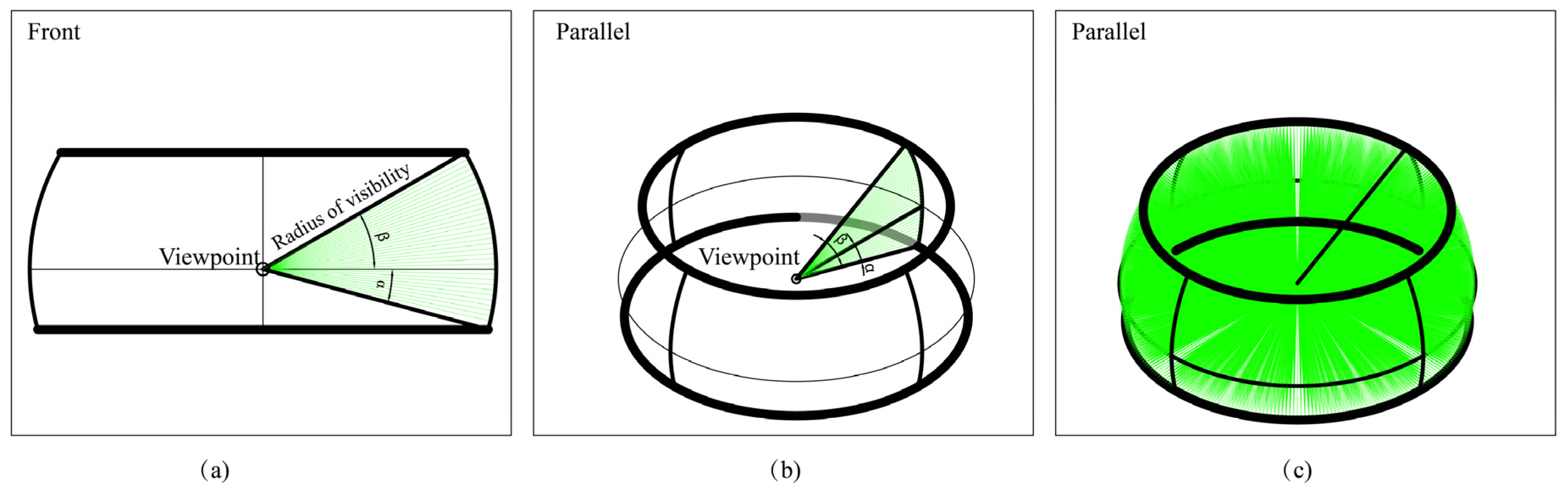
3.1. 3D Isovist-Based Landmark Visibility Measurement Method

Algorithms using 3D isovists achieve the visibility of landmarks measured from all decision nodes, as a fundamental condition for 3D NL GAM construction. In this study, the 3D isovist component on Rhino 7.0 and Grasshopper software platforms is used to generate 3D isovists located at the viewpoint of the decision node. In the software platform, a 3D isovist is represented as a line-of-sight structure originating from a viewpoint, and is generated according to the viewing direction, viewing range, and line-of-sight generated density, parameter settings, etc. In the process of wayfinding, people adjust the direction of their head’s rotation, so that a horizontal viewing range of 180° can usually be reached [81]. When a decision point is reached, it is possible to turn around and identify the surroundings. Thus, the horizontal viewpoint can reach 360°, and this field of view is defined as the panoramic 3D isovist [39]. The vertical viewpoint includes the vertical downward viewpoint α and the vertical upward viewpoint β. In the vertical viewing, the color of the visible object is not easily perceived when the upward viewpoint β is greater than 30°, and people are more accustomed to the viewpoint centerline, which is generally directed downward by 10° when standing to ensure the safety of traveling [40]. Thus, β = 30° was taken. Although the actual downward perspective is often greater than the upward perspective because the viewpoint is very close to the ground, the visible volume is smaller, thus, we set α = 15 °.
In an ideal state without occlusion, the panoramic viewshed of the viewpoint consists only of equidistant lines of sight at a set viewing range (Figure 2), forming a sphere with the radius of the length of the line-of-sight. Figure 2a,b represent a vertical sector view. Taking the angle between the vertical lines of sight as 1°, the number of lines of sight of a vertical sector is α + β roots. Rotating the vertical sector by 360° horizontally and copying one vertical sector every 1° forms the structure of a panoramic field of view (Figure 2c). Then the total number of lines-of-sight (Tlos) of the ideal field of view is:
T l o s = 360 × ( α + β + 1 )
Subtracting the area of the upper and lower crowns from the area of the sphere, it follows that the visible area represented by the end of each line-of-sight is:
A l o s = π R 2 ( sin α + sin β ) 180 ( α + β + 1 )
where Alos: the visible area of each line-of-sight; R: the length of the line-of-sight.
In a line-of-sight obstacle environment formed by a 3D geometry model, the panoramic viewshed is divided into three line-of-sight types:
  • No obstacle line-of-sight: the initially set viewing range is maintained, representing the visibility of the sky;
  • Ground line-of-sight: line-of-sight projected onto the ground;
  • Obstructive line-of-sight: line-of-sight is obstructed by geometry. At the same time, the reference number and length of the line-of-sight, as well as the reference number of the geometry onto which the line-of-sight is projected, are recorded in the 3D isovist dataset.
Since the obstructed environment only changes the length of the initial line-of-sight distance and does not change the density of lines-of-sight in the 3D isovist, the visible area at the endpoint is only related to the length of the line-of-sight. In Equation (4), the visible area expressed by the endpoints of every line-of-sight projected onto a landmark is cumulatively the visual area of that landmark corresponding to the decision node.

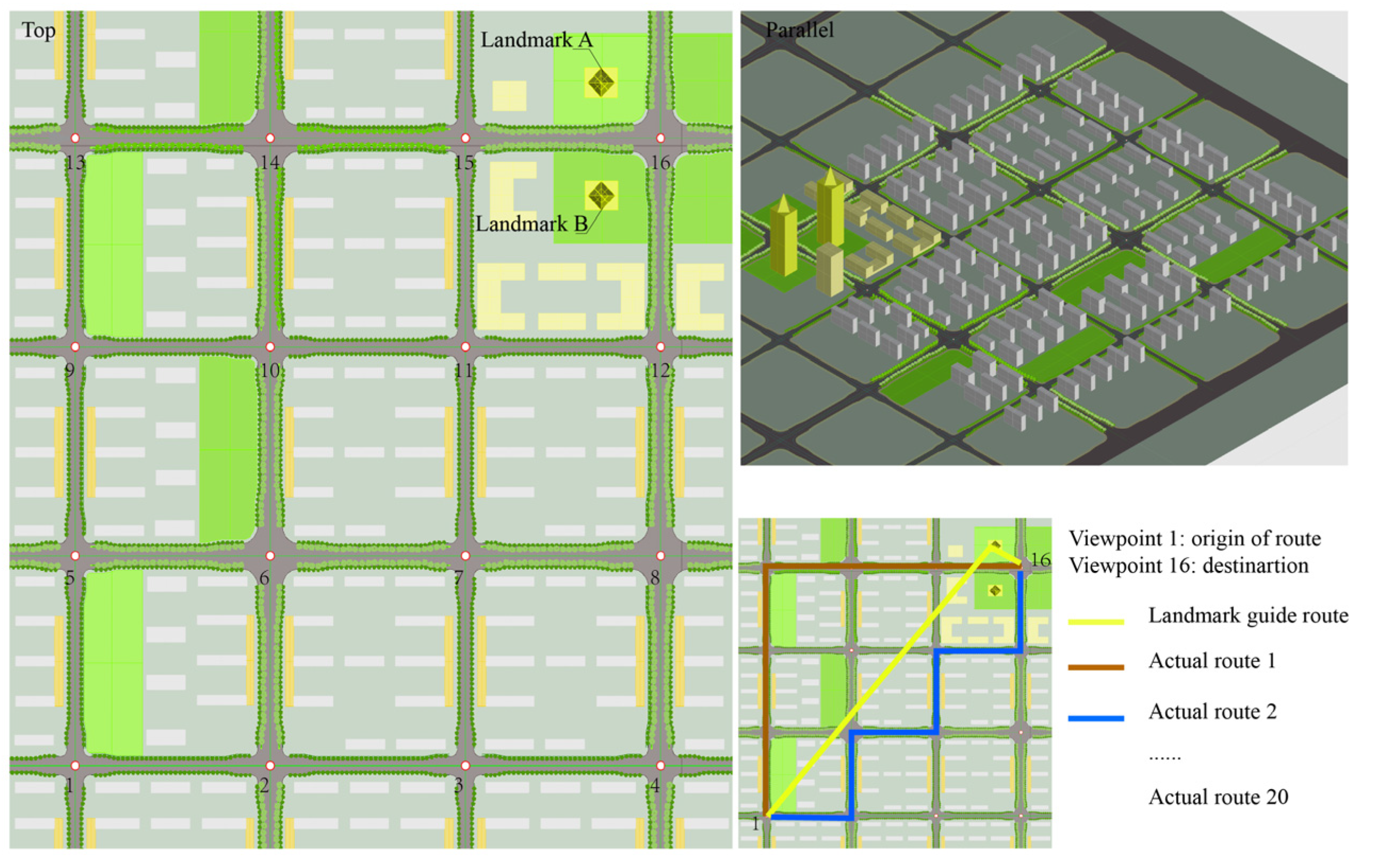
3.2. Simulation Model of a Standard Urban Neighborhood

A standard residential neighborhood (10 min walkable range) model (Figure 3) was simulated in the Rhinoceros3D platform to express the 3D NL GAM construction process. The area of the simulated neighborhood was about 100 hm2, the average number of floors of all residential buildings was 10, and the population size was 30,000, which comprised a typical compact urban neighborhood. The urban spatial form is the external appearance of the urban tissue, which consists of four categories of geometric models: natural landscape resources, residential buildings, public buildings, and urban public facilities, etc., which are subdivided as follows:
  • Natural landscape resources: mountains, forests, rivers, lakes, etc., within the city;
  • Neighborhood blocks: urban residential area units made up of residential building groups;
  • Public buildings: civic buildings of various functional types, including office buildings, shopping malls, hotels, conference centers, etc.
  • Urban public facilities: streets, sidewalks, street trees, parks, squares, parking lots, etc.
Analyzing the street space from a 2D grid alone makes it difficult to determine a way-finding path and can easily lead to getting lost. The block consisted of eight streets with sixteen street intersections. This arrangement made it difficult to distinguish the path orientations of the street intersections and resulted in too many undetermined paths. For example, if intersection 1 is the starting point and intersection 16 is the ending point, and each crossing is counted as 1 topological distance, then the shortest path distance is 6 topological depths, and 20 shortest paths can be arranged.
Landmark-based route selection methods can better reproduce human navigation [14]. It can be seen in Figure 3 that if Landmark A is visible from intersection 1, the shortest path guided by the landmark is V1-Landmark A-V16, i.e., the topological distance of the landmark-guided path is 2. Thus, with the intervention of landmarks, the choice of route intersection becomes less important, and the choice of any actual path does not lead to getting lost but only toward the landmark, and the destination can be reached by walking in the direction of the landmark. Therefore, to implement landmark intervention analysis, it was necessary to determine the setting of the path decision node and the landmark visibility at the decision node.

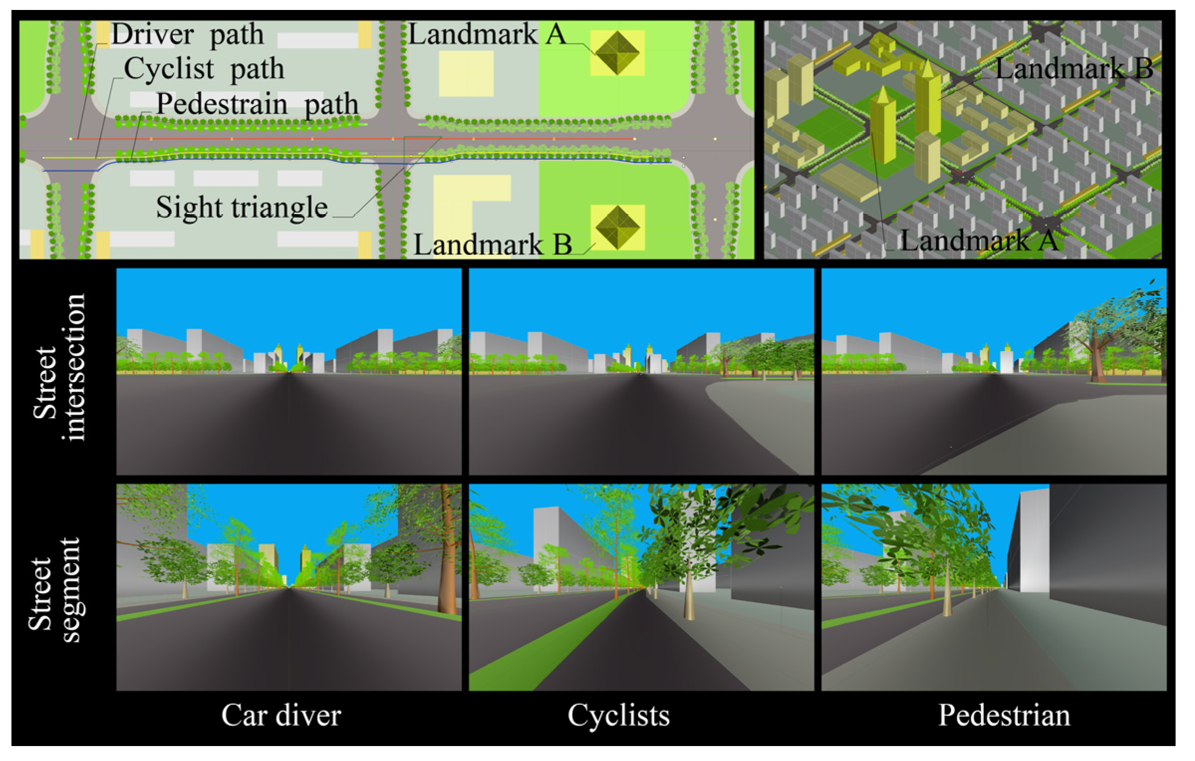
3.3. Determination of Path Decision Nodes in 3D Grid

Determining path decision nodes for wayfinding or navigation in urban space is the first task in constructing 3D NL GAM. Firstly, the visibility differences between road sections and intersections were dynamically simulated in a 3D environment (Figure 4). The method involved route selection and parameter setting for walking, cycling, and driving [74], and arranging motor vehicle lanes, bicycle lanes, street trees, and sidewalks in a street environment, as follows:
  • The trees on either side of the trail were spaced 8 m apart and had a net height of more than 2.8 m below the branches of the canopy;
  • The pavement trees were spaced 6 m apart, with a net height of more than 1.8 m below the crown branches;
  • The line-of-sight triangle was set at the intersection.
Then, using Rhino 7.0 3D model-making software, a dynamic snapshot was set up with a camera focal length of 12 mm and the shot direction facing the next viewpoint:
  • The height of the walking viewpoint was 1.6 m from the ground, the distance between the viewpoints was 30 m, and the playing speed of the dynamic snapshot corresponded to the walking speed of the person, which was 5 km/h;
  • The riding viewpoint was 1.75 m from the ground height, the viewpoint spacing was 30 m, and the playback speed of the dynamic snapshot corresponded to the riding speed, 10 km/h;
  • The driving viewpoint height from the ground was 1.35m, the viewpoint spacing was 50 m, and the playback speed of the dynamic snapshot corresponded to the speed of the motor vehicle, 20 km/h.
Thirty-two architecture students were assigned to view dynamic snapshots to compare the differences in landmark visibility between the 3 path types (Figure 4). The results indicated that the intersection enabled more visible information to be obtained. At the intersection location, on the one hand, the road was visible in both directions, and on the other hand, the street trees were less obscured by the city buildings. When in the roadway area, only one road was visible, and street trees were highly obscured by buildings. Figure 4 shows that two landmark buildings can be seen in the distance at the intersection, but the visibility of the landmark buildings in the section area was significantly reduced. It follows that the intersection location should be identified as the decision node, and the intersection point of the road medians is taken to express the logical space of the intersection.
In addition to the intersections, additional decision nodes should be created in accordance with the axial graph analysis principle. This indicates that the urban grid should satisfy line-of-sight continuity, and the decision nodes should be set at the locations where line-of-sight transitions are generated. The decision nodes were required as follows:
  • Street intersections and street turns within the analysis area are decision nodes of the 3D grid;
  • For arc roads, consecutive decision nodes should be set and the maximum spacing requirement should be satisfied;
  • For roads with significant slopes, the decision node should be set at the top of the slope;
  • When two roads intersect, path continuity can only be formed by secondary roads.

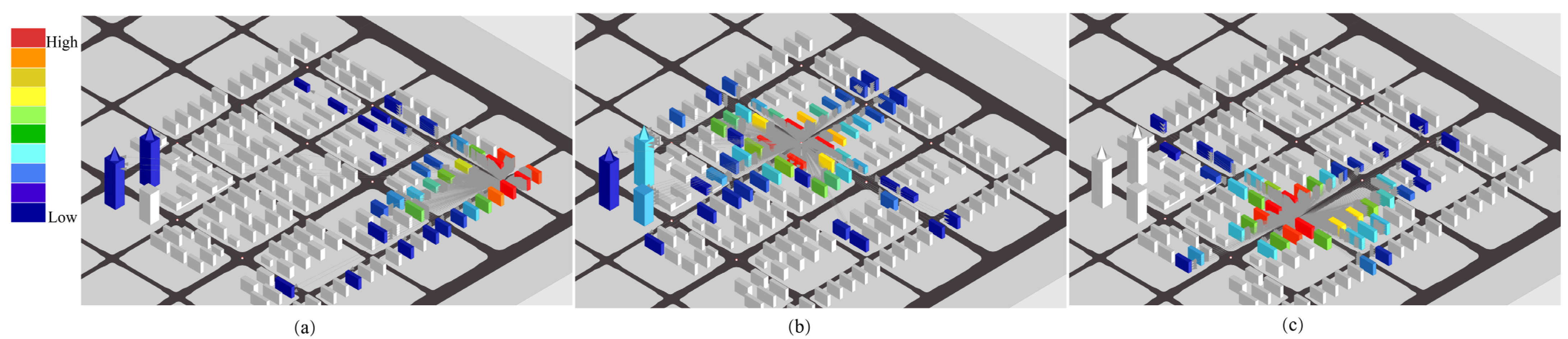
3.4. Expression Functions for Landmark Visibility in 3D Grid

Landmark visibility measurement consists of two objectives; one is the visibility of the decision point to the landmark, and if it is visible, the decision point forms a connection with the landmark. The other objective is to measure the visible area of the landmark and the distance of the decision point from the landmark if the landmark is visible, and to quantify the dominance of expressing the visibility of the landmark.
Computation of the viewing data of the decision nodes in the standard urban neighborhood environment was performed by running the dynamic parameters program with the 3D isovist component on the Rhino 7.0 and the Grasshopper software platforms. The ideal viewing range was set to 5000 m, the horizontal view angle was 360°, the vertical view angle was 45°, and the viewpoints and obstacles were picked up. After the 3D isovist component calculation, the visible data of 16 decision nodes were obtained (Figure 5). The data consisted of various types of lines of sight, and each viewpoint accumulated a total of 16,560 lines-of-sight. To facilitate landmark visibility, only the obstructive sightlines are shown in Figure 5, which shows that the greater the number of projected sightlines of the geometry, the warmer the displayed color of the geometry and, with fewer sightlines, the cooler the displayed color. Based on the corresponding values of the length of the sightlines and Equation (4), the visible areas of the viewpoints to the two landmark buildings were obtained for all decision nodes (Table 1).
Landmark visibility dominance is an expression of the visual perception of landmark visibility at the decision node location. The main influencing factors of people’s visual perceptions of landmarks include visual acuity, sight distance, and visible area [82]. The initial setting of the 3D isovist is a constant viewing range; that is, the volume of the panoramic field of view is consistent within the same urban area, representing a normalized field of view. Thus, the comparison of visual perception metrics for different landmarks at a decision node is achieved in the same normalized viewshed. That is, the landmark visibility metric is directly expressed as a function of the visibility area of the viewpoint to the landmark and the view distance:
V I S I B I L I T Y i = A l m D s i g h t + 1
VISIBILITYi: landmark visibility index; Alm: landmark visible area; Dsight: average length of lines of sight.

4. Salience Computation of Structural Landmarks in Urban Neighborhood

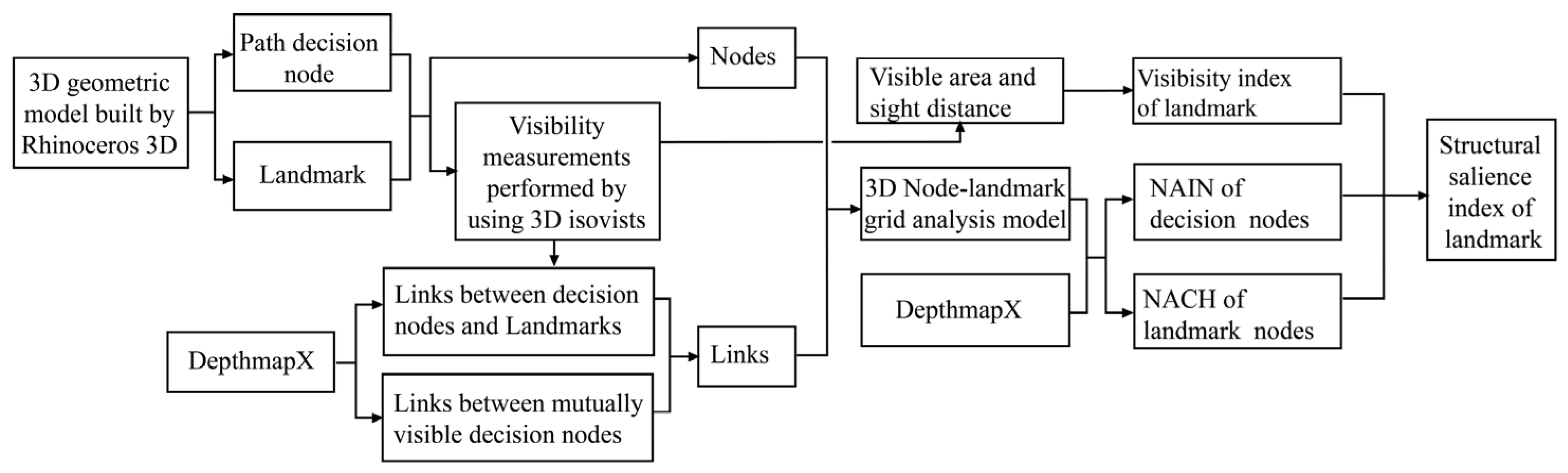
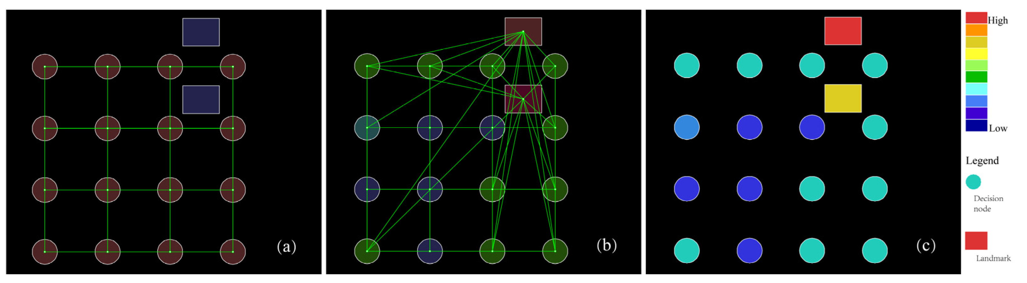
4.1. Computation of Structural Landmark Salience

The decision node locations and landmark visibility measurements were determined to form a 3D NL GAM, which was used to compute the spatial mobility properties of node and landmark locations. The computation of the spatial properties in this paper is performed on the DepthmapX software, that is, after importing the spatial node data obtained in the Rhino and Grasshopper software platforms into the DepthmapX software platform, the grid analysis model is further constructed and computed in the DepthmapX software. To illustrate the differences before and after landmark intervention in the grid, the changes in the spatial movement attributes of nodes and landmarks in the GAM were compared for the unlink and link cases (Figure 6, Supplementary Materials Table S1). In the unlink case (Figure 6a), it expressed only a 2D node link. The VGA result indicated [61,83] that the NAIN value for all intersections was 1.16. Thus, it was difficult to determine if there was any difference in the spatial mobility properties of the decision nodes from the 2D grid alone. Based on the landmark visibility measurements of the 16 decision nodes determined with the 3D isovist method, the link between nodes and landmarks was established (Figure 6b). In this case, the spatial movement attributes of both landmarks and nodes reflected significant differences (Figure 6c).
While the decision node was concerned with spatial accessibility, the landmark location was concerned with spatial selectivity; that is, the NAIN of the decision node and the NACH of the landmark location were obtained for the 3D NL GAM using the space syntax principle. According to the multiplier effect of grid grouping [33,44,45,46], the greater the NAIN of the nodes of the path decision point location and the higher the number of people gathered at this place, the greater the influence of landmarks. At the same time, higher NACH values of landmark location nodes indicate that the landmarks are also more directional along the wayfinding route to the destination. However, there is a special case where the decision node, destination, and landmark are adjacent to each other (all decision points that have a view of the landmark are in the same straight-line street), and the NACH of the landmark is zero. From the grid effect, landmarks with a degree of zero are named as local landmarks. Thus, for a decision node, the structural salience of a landmark is computed as follows:
S S L i = ( N A I N i × V I S I B I L I T Y i ) × ( N A C H l m + a )
where SSLi: structural salience of a landmark corresponding to path decision node i; NAINi: normalized angular integration of path decision point location nodes; VISIBILITYi: landmark visibility index; NACHlm: normalized angular choice of landmark location nodes; a: initial bootstrap effect constant of local landmarks.
Having determined the landmark salience values for each decision node (Figure 7), it was possible to compare the advantages of the locations of the landmarks in the grid with the locations of the decision nodes. The values of each structural landmark salience-related factor in the standard neighborhood NL GAM were substituted into Equation (6) to obtain the landmark salience for the 16 viewpoints (Figure 7a). The structural salience of a landmark in the grid was the average of the salience of the landmark with respect to all decision nodes in the grid for all decision nodes. The structural salience of Landmark A was 6.24 and that of Landmark B was 5.99 (Figure 7b).

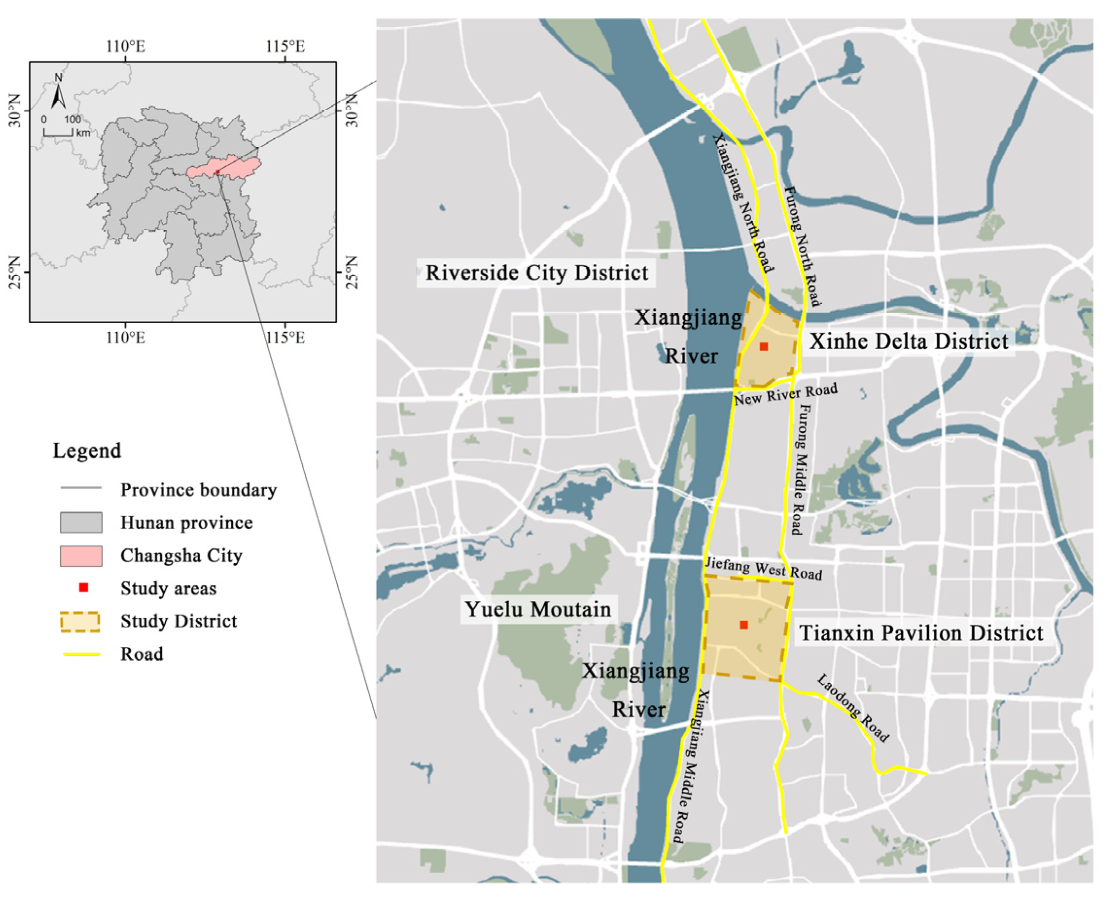
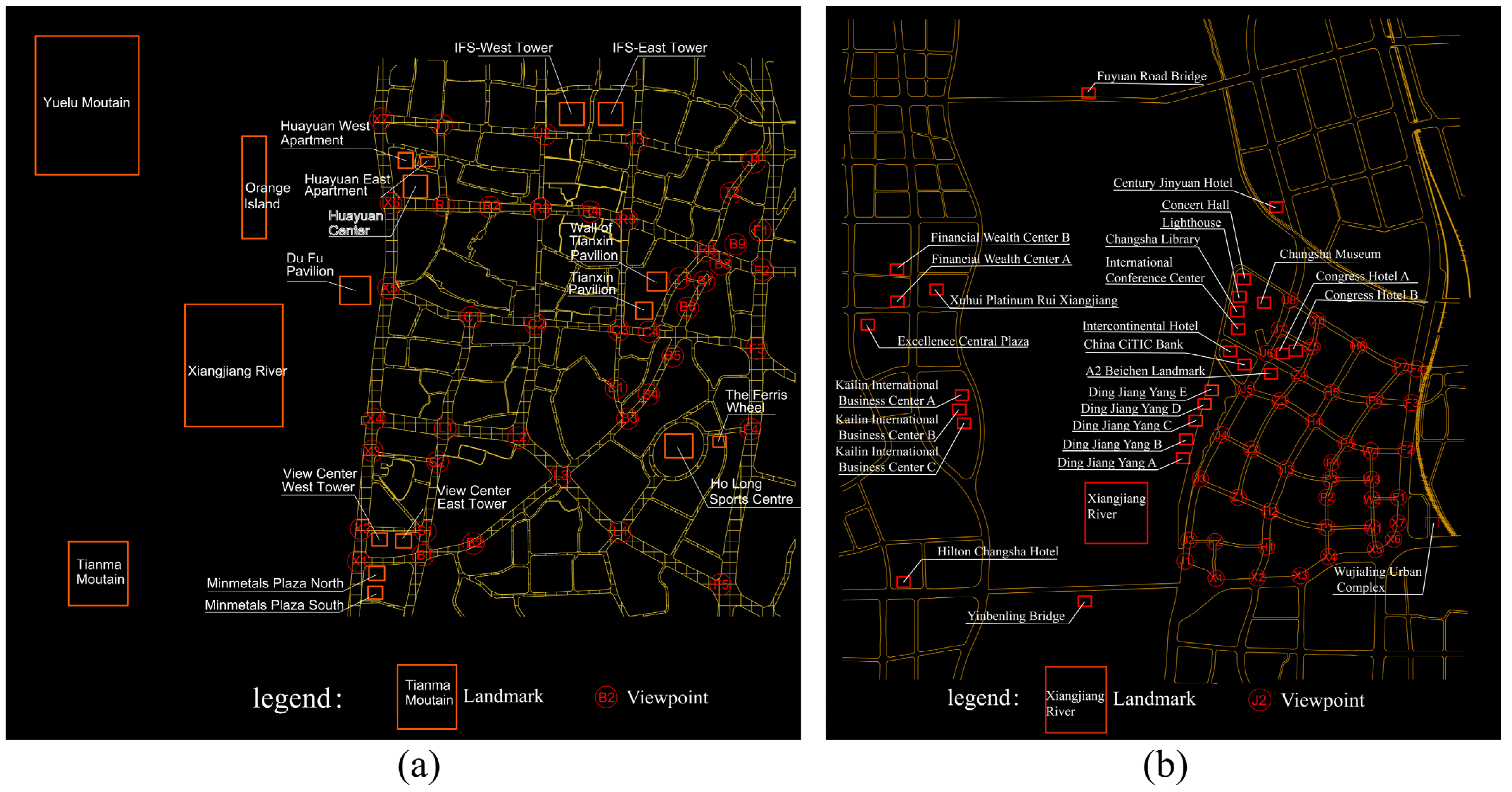
4.2. Computation Procedure of Structual Landmark Salience for Two Typical Samples of Districts in Changsha

A typical urban sample area is a compact urban residential area with a 15 min walkable living radius, typically around 400 hectares. It has distinct natural and architectural landmarks within its viewing area. At the same time, the building groups in the area have the typical spatial form of a compact city. In this paper, two tracts located in Changsha, Hunan, China (Figure 8, Table 2) were selected, which are the Tianxin Pavilion District (TP-District) (Figure 9) and the Xinhe Delta District (XD-District) (Figure 10), which two urban areas in Changsha, China, and both are typical high-density compact urban neighborhoods along the riverfront, with significant spatial morphological differences between them (Table 2). Table 2 presents the basic situation of the two zones. The landmarks in the area were initially identified based on natural landscape resources, human resources, building volume, building height and architectural shape [11,28]. The final landmark analysis objects were identified based on relevant public results from the Changsha Planning Information Center combined with expert consultation recommendations. In this study, three types of 3D NL GAM were established based on the morphological features of each neighborhood:
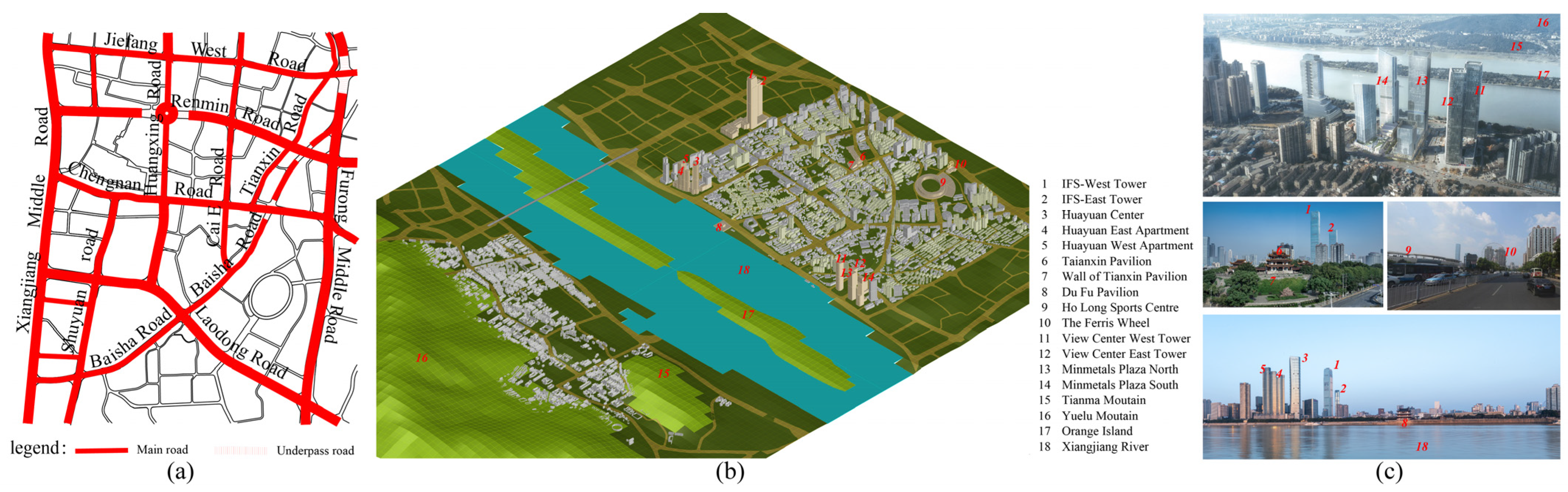
  • TP-District, an area typically formed by a combination of high- and low-rise architectural groups;
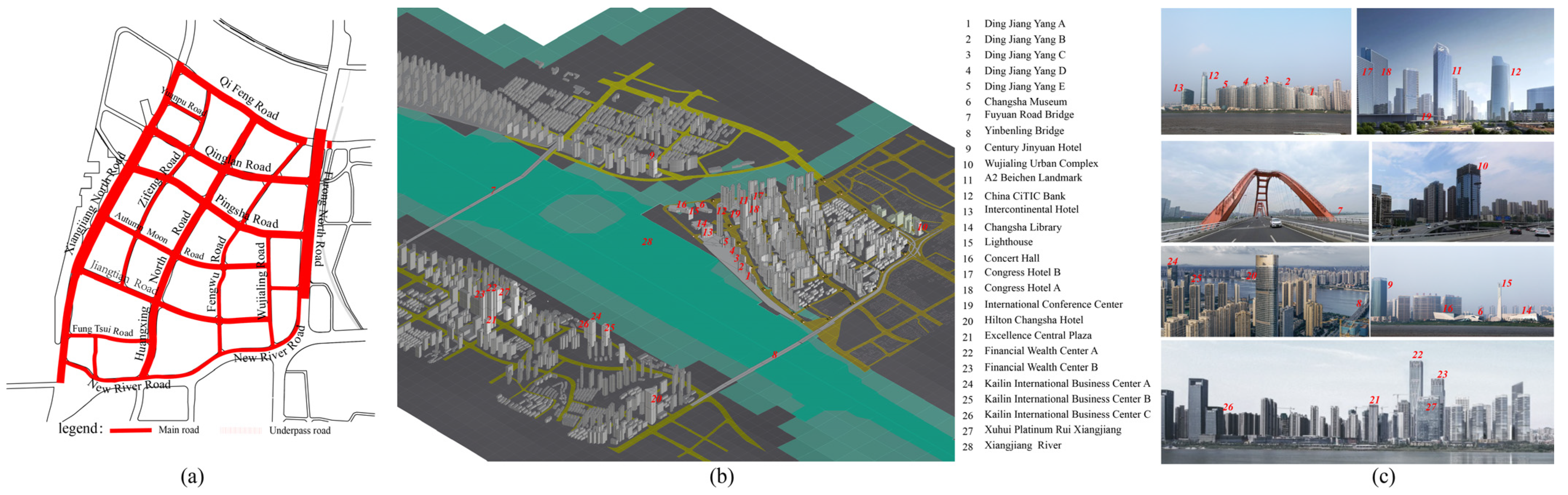
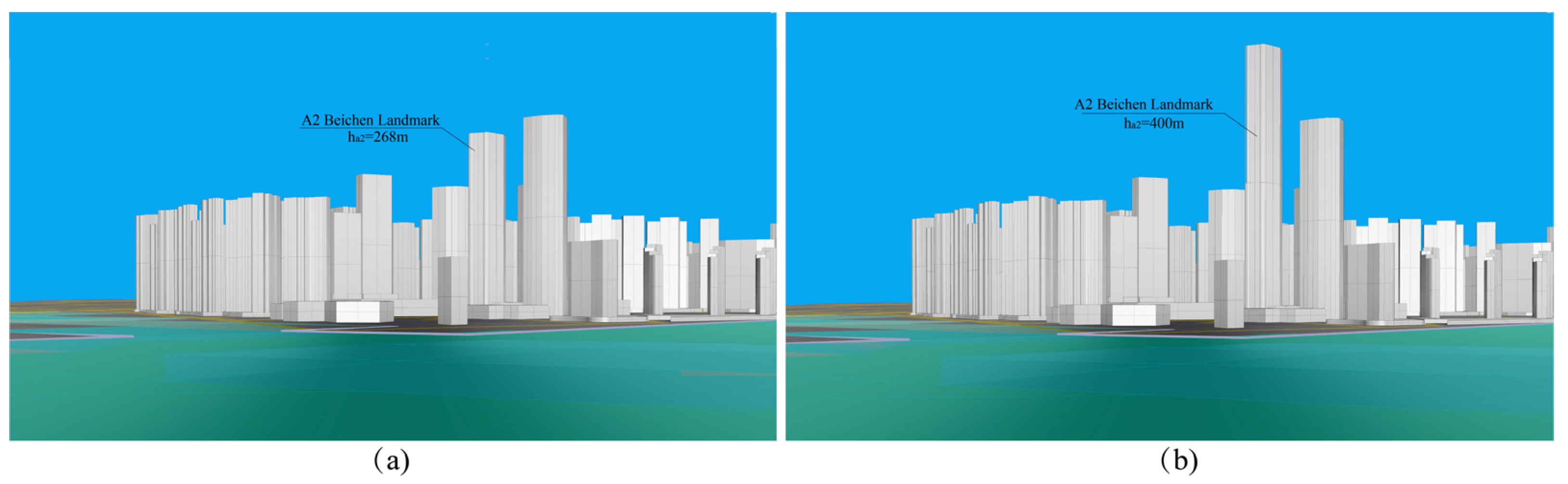
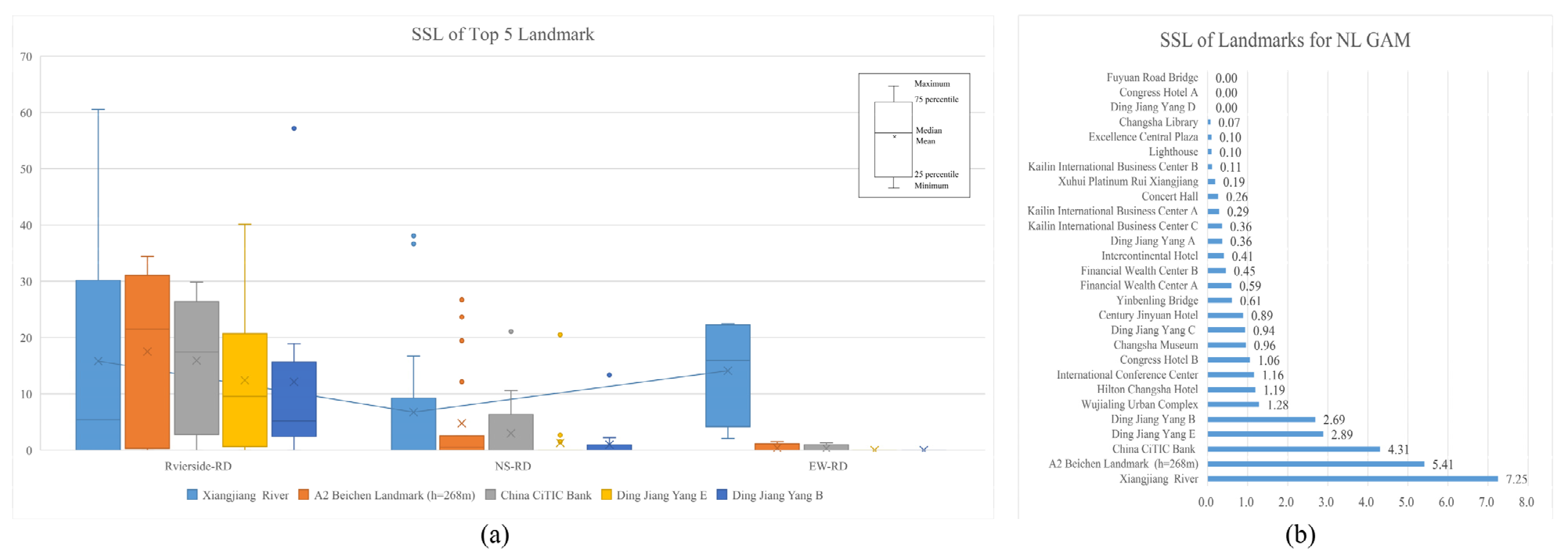
  • XD-District, a typical area pattern formed mainly by high-rise building groups; the height of the proposed A2-Beichen Landmark was 268 m (Figure 11a), with Ha2 = 268 m as the default in the later text;
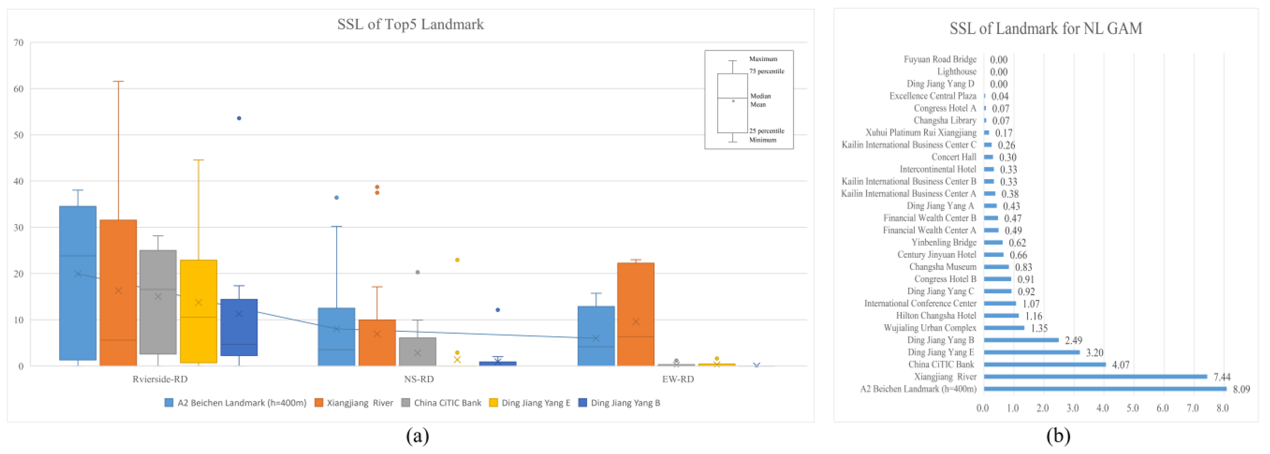
  • For the XD-District, the height of the proposed A2-Beichen Landmark was set at 400 m (Figure 11b), with Ha2 = 400 m as the default in the latter part of the text.
Computation of structural landmark salience for the above three morphologies of urban areas was needed to achieve three research objectives: First, we compared the structural salience differences between landmarks in the two types of neighborhoods with the combined architectural group morphologies. Second, quantitative results were used to compare the structural salience of large-scale natural landscapes, super-tall architectural landmarks, multistory buildings, and human landmarks. Finally, we analyzed the effect of changing the morphology of individual building landmarks (A2-Beichen Landmark) on the structural salience of landmarks.
We followed the steps below to build the 3D NL GAM for computing the structural salience of landmarks in the grid:
Step 1: Make a 3D model of each urban district. On the ArcGIS platform, geographic information data are formed based on raster images of terrain and building vector data. Then, these are converted to a DXF vector data format, and imported into the Rhino 7.0 3D software platform, in order to generate the 3D model (Figure 9b and Figure 10b).
Step 2: Determine the landmarks of the area. Landmarks of urban districts include both neighboring landmarks and distant landmarks.
Step 3: Determine the decision nodes. The decision node number is set according to the name of the main road where the decision node was located and classified as a riverfront road decision node (Riverside-RD), north–south road decision node (NS-RD), east–west road decision node (EW-RD), or north–south to east–west road decision node (NS-EW-RD). Cumulatively, there are 44 decision nodes in the TP-District (Figure 12a) and 43 decision nodes in the New River Delta area (Figure 12b).
Step 4: Measure landmark visibility for all path decision nodes (Figure 13). On the Grasshopper platform, the initial setup parameters of the 3D isovist are kept consistent with those of the standard urban neighborhood model, and a dynamic program is written to record and filter the sightline data projected to different landmarks from each viewpoint, as well as to calculate the visibility of landmarks according to Equation (5).
Step 5: Calculate the movement attribute of node space (Figure 14). The 3D NL GAM is formed by establishing relationships between route decision nodes and between decision nodes and landmarks. Perform the graph analysis operation on the DepthmapX platform, edit the node normalized angle integration degree attribute according to Formula (1), and edit the node-normalized angle choice degree attribute according to Formula (2).
Step 6: Calculate the structural salience of the landmarks. Calculate the structural salience of landmarks corresponding to each decision node according to Formula (6) and calculate the structural salience of landmarks in the whole grid system.

5. Results

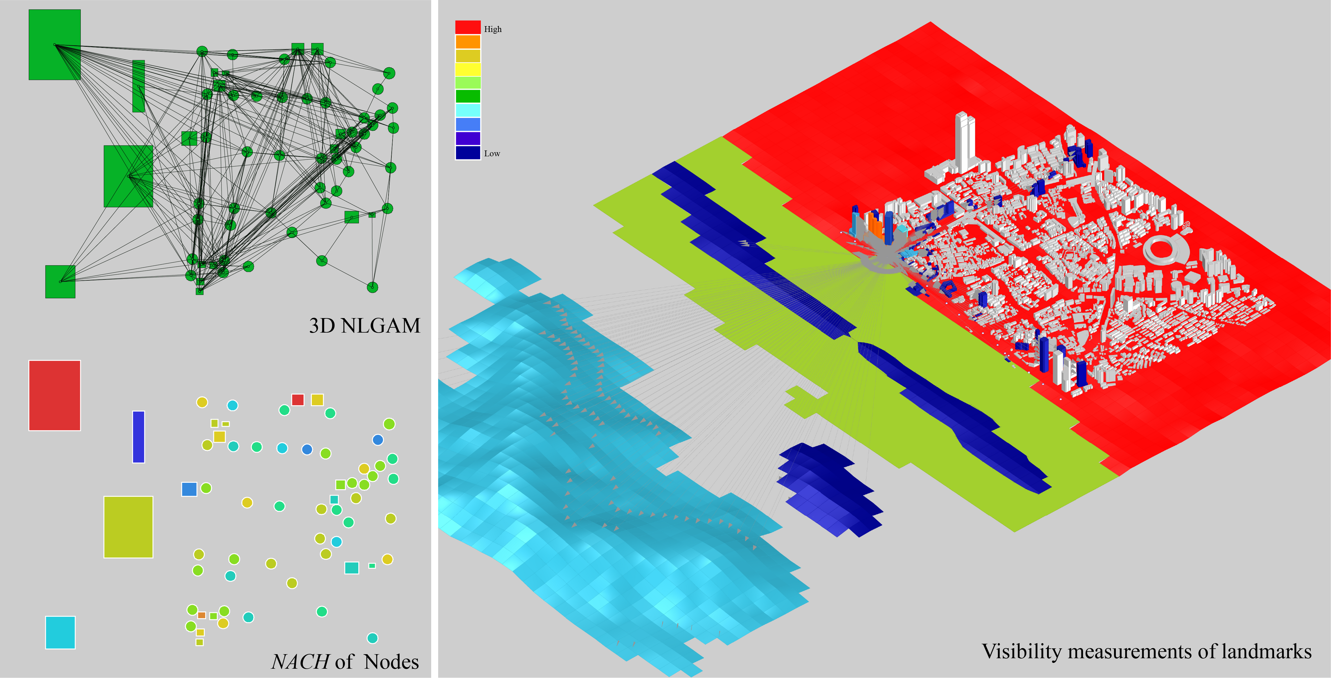
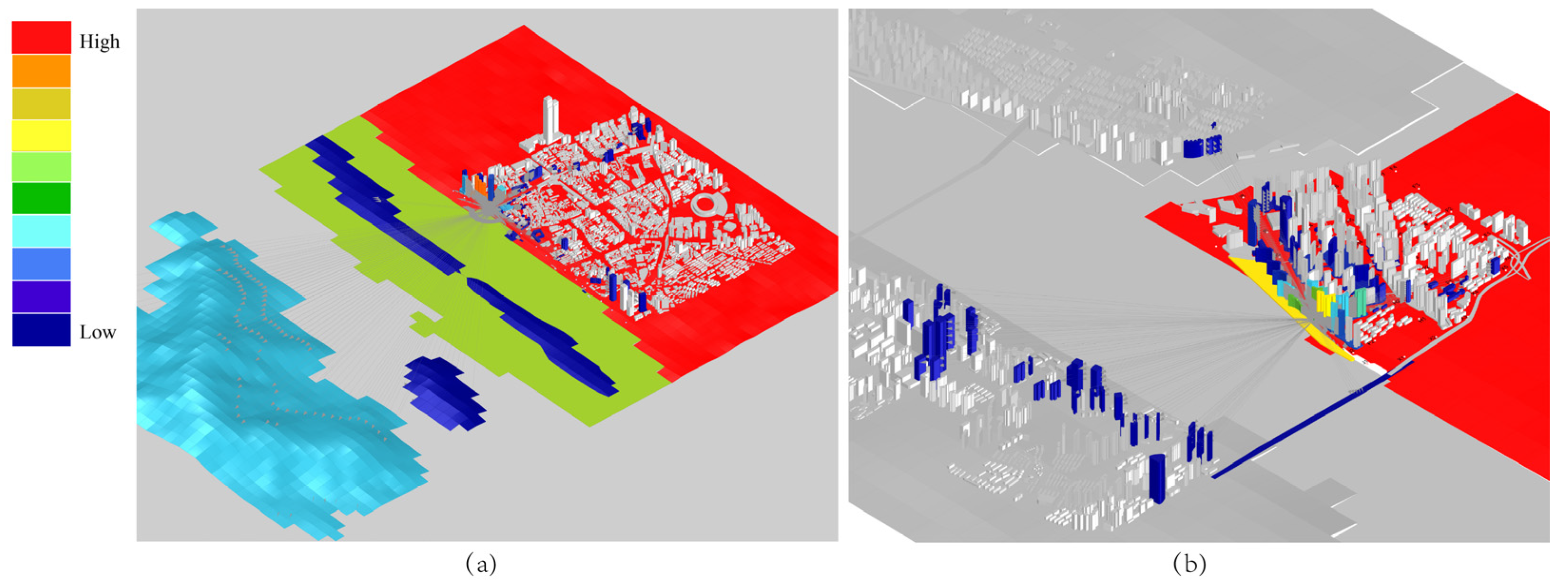
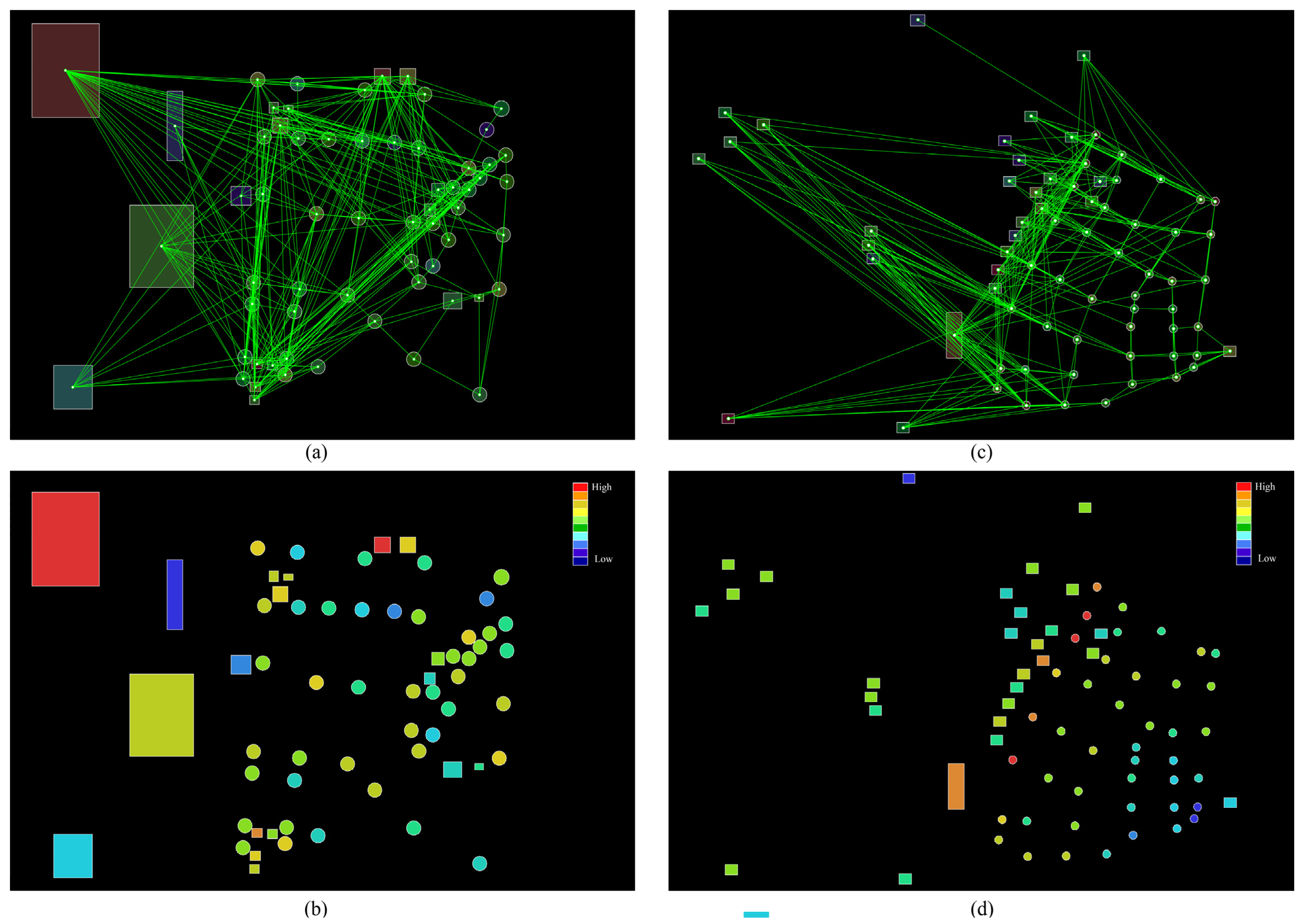
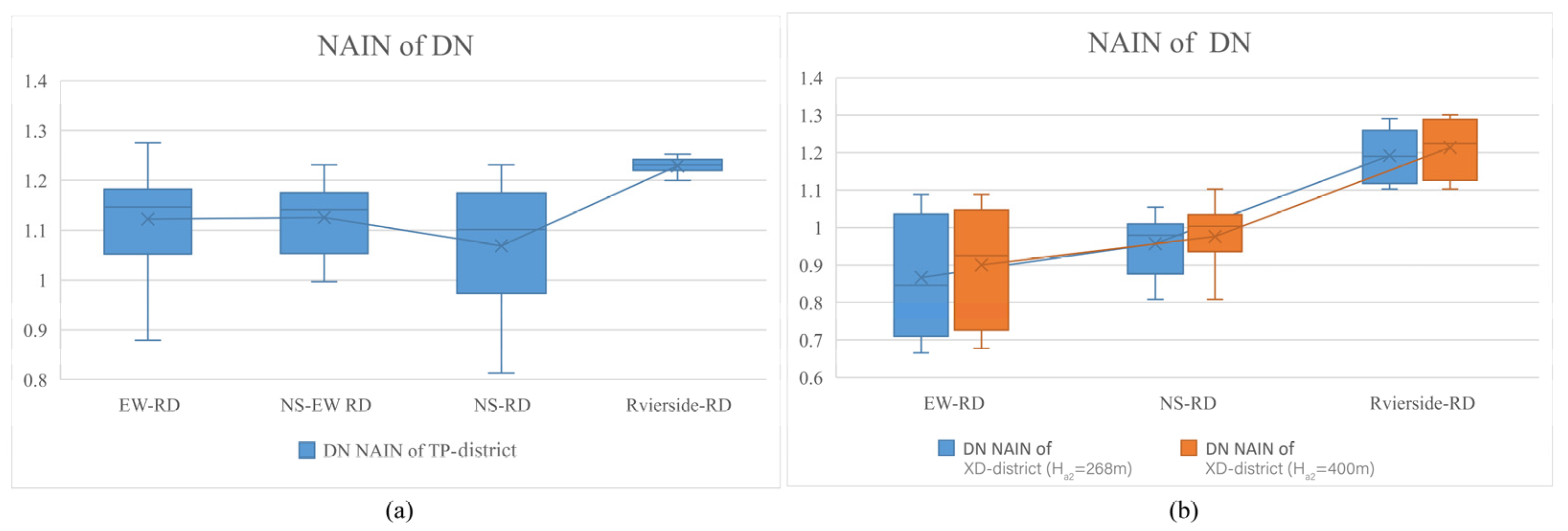
5.1. Spatial Movement Properties of 3D NL GAM

When comparing the NAIN values of the three grid decision nodes (Figure 15, Tables S2–S4), the TP-District had obvious advantages. The average NAIN value in the TP-District was 1.128; when Ha2 = 268 m, the average NAIN in the XD-District was 0.984, and when Ha2 = 400 m, the average NAIN in the XD-District was 1.006. This indicated that the route decision nodes in the TP-District had better accessibility and were suitable for keeping. Increasing the height of landmarks, which increased the connection between decision nodes and landmarks, improved the NAIN values of nodes. The connection data indicated that the A2 landmark increased from 268 to 400 m with the addition of only three links, and the improvement in NAIN was not significant.
The integration of decision nodes in the TP-District was relatively concentrated, and the grid was uniform. The box plot (Figure 15a) of the integration of the decision nodes and the standard deviation (Table 3) of various types of data demonstrated that the decision nodes along the Riverside-RD had a wide field of view on its west side, and their integration maintained the maximum value in the system, as well as the most concentrated numerical range. The values for the NS-EW-RD were relatively consistent and at a moderate level. The values for the NS-RD were relatively scattered, with low mean and median values.
The NAIN values of decision nodes in the XD-District were relatively scattered. The box plot (Figure 15b) and the standard deviation (Table 3) of the data of each type of decision node indicated that the NAIN values in both cases were relatively scattered, and the data were located in a large range. The NAIN values of the path decision nodes along the Riverside-RD remained at the maximum value in the system but they were more scattered than in the TP-District. Although the decision nodes of the NS-RD had the largest number of nodes, their NAIN values were relatively concentrated, with mean and median values close to one. The NAIN values of the EW-RD were scattered, and most of the values were less than one; that is, the node space was relatively isolated.
After increasing the height of the A2 landmark in the new 3D NL GAM, the NAIN values of a few decision nodes remained unchanged, while the NAIN values of most decision nodes were improved. In particular, the NAIN values of the three nodes that gained visibility of the A2 landmark because of its elevation were significantly enhanced.
Comparing the landmark NACH values of the three 3D NL GAMs (Figure 16, Tables S2–S4), the TP-District still maintained a clear advantage. The average value of landmarks in the TP-District was 0.789; when Ha2 = 268 m, it was 0.595 for the XD-District and when Ha2 = 400 m, it was 0.573 for the XD-District. That is, the TP-District landmarks had higher NACH values, indicating that landmarks in this area were more guided. Increasing the height of the landmarks changed the structural relations of the grid, but the results indicated that the mean NACH value of the landmarks decreased instead.
The results of the box plot (Figure 16) and standard deviation (Table 4) indicated that the NACH data of the TP-District landmarks were more dispersed, and the guiding of landmarks had obvious variability. High-rise buildings maintained larger NACH values in the system and remained within a more concentrated range of values, with the IFS-West Tower having the highest NACH value of those in the grid. Although there were only five natural landscape landmarks, the NACH value interval of landmarks was large and the data dispersion was high, among which the NACH value of Yuelu Mountain was second only to that of the IFS-West Tower, but the NACH value of Orange Head was zero, the smallest value in the grid. The number of humanistic landmarks was smaller, and the connections with decision nodes were lower. Their landmark NACH values were all lower, and the data were more concentrated.
The NACH values of the landmarks in the XD-District were more scattered in both cases. The Xiangjiang River was the only natural landscape landmark in the area, and its NACH value was second only to the Beichen-A2 landmark. For the neighboring high-rise landmarks, the data lay in a larger dispersion interval, and their mean and median values were only lower than those of the Xiangjiang River. For distant high-rise landmarks, the NACH value interval remained low, even though they were all ultra-high-rise buildings. Cultural landscape landmarks had lower NACH values and more scattered data.
After raising the height of the Baichen-A2 landmark, the NACH was first significantly increased, and the NACH values of most of the nearby high-rise landmarks were raised. However, this also lowered the NACH values of most of the distant high-rise buildings, as well as those of the area’s cultural landmarks.

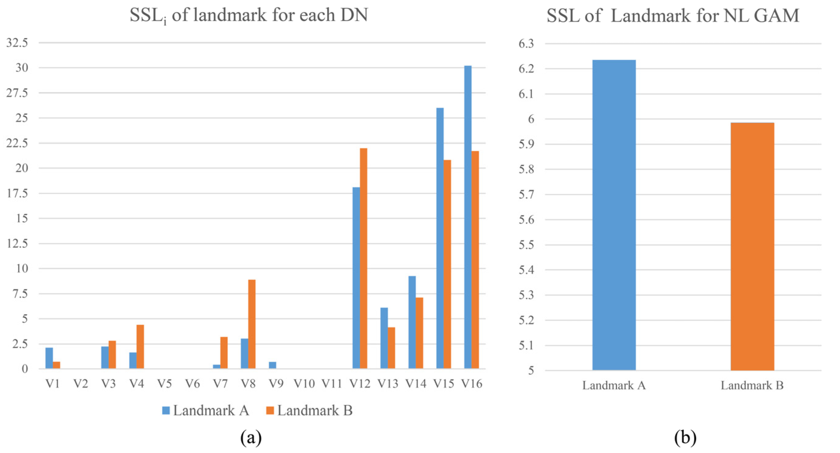
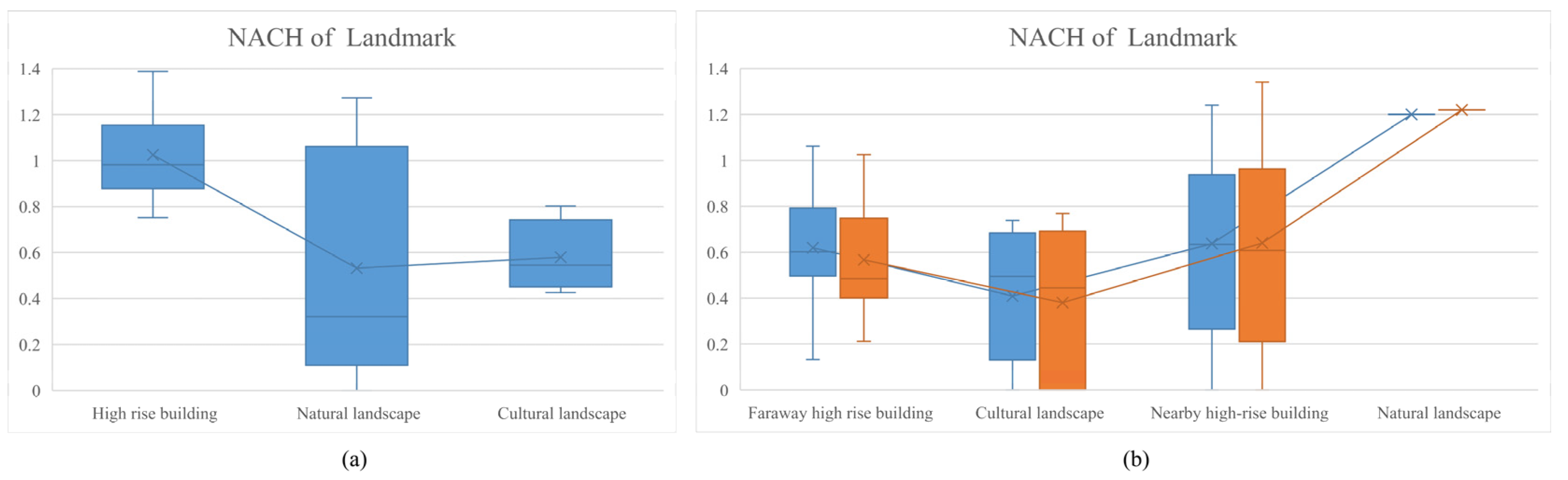
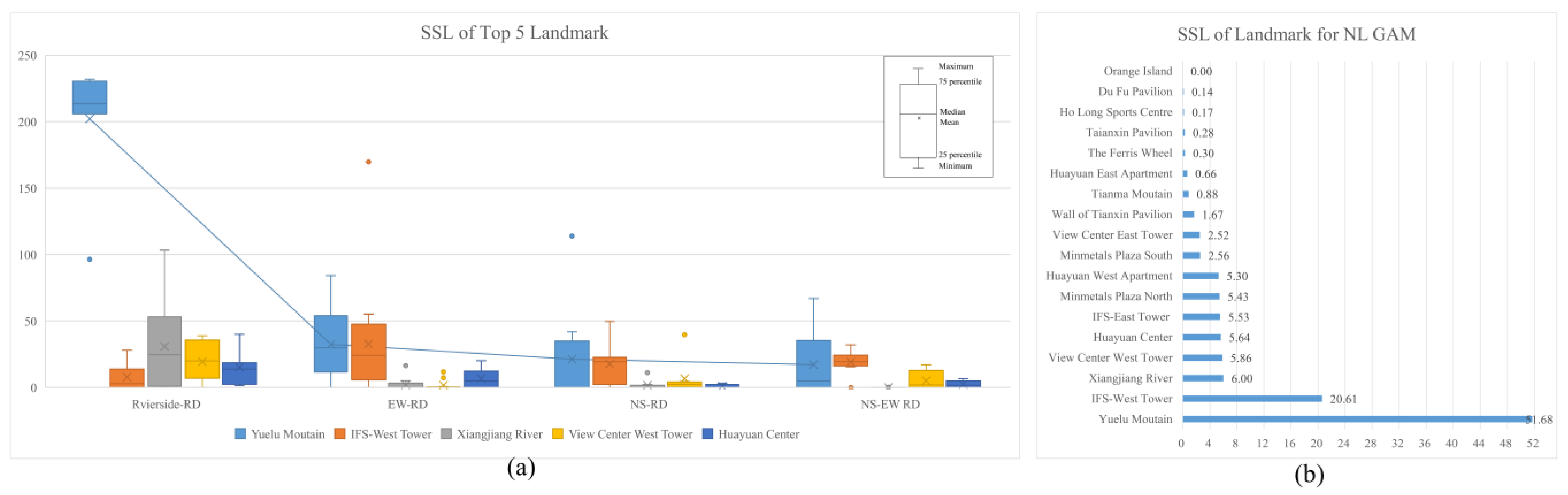
5.2. Structural Salience of Landmarks

The landmark visibility values at each node were calculated according to Equation (5), and the structural salience of the landmarks was then calculated by substituting Equation (6). The results of the TP-District (Figure 17, Table S2) and XD-District (Figure 18 and Figure 19; Tables S3 and S4) expressed the structural salience of landmarks in the area with a combination of high- and low-rise building groups, and in the area dominated by high-rise building groups, respectively. The calculated results indicated that the mean value of landmark structure salience was 6.402 for the TP-District and 1.211 (Ha2 = 268 m) and 1.291 (Ha2 = 400 m) for the XD-District. This meant that the landmark salience of the TP-District was much larger than that of the XD-District, and raising the height of the landmark improved its own salience and that of the area.
In the TP-District, the structural salience of all landmarks had a large range of values, with a median of 2.54. The structural salience of Yuelu Mountain and IFS-West Tower was definitely dominant, with Yuelu Mountain being the largest. Yuelu Mountain could be seen from 29 of the 44 path nodes, mainly those along the EW-RD, including Xiangjiang Middle Road, Jiefang Road, Renmin Road, Chengnan Road, and Baisha Road. Although the IFS-West Tower was visible from 30 nodes, the building’s visibility was not comparable to that of a large-scale natural mountain. Thus, the structural salience of the IFS-West Tower was the second-highest in GAM. The structural salience of the Xiangjiang River was much lower than that of the Yuelu Mountain, with only 15 nodes visible to the Xiangjiang River, ranking third. High-rise buildings had a high structural salience, with most of them ranking above the median. Cultural landscape landmarks had lower structural salience and ranked below the median.
In the XD-District, the structural landmark salience of the Xiangjiang River ranked first when the Baichen-A2 landmark Ha2 = 268 m (Figure 18). There were 11 high-rise buildings in the neighboring landmarks, and although the top five architectural landmarks were all neighboring landmarks, four of them were also ranked below the median, indicating that the structural salience of high-rise buildings in the neighboring landmarks was obviously less advantageous than that in the TP-District. For the distant landmarks, there were four super-high-rises that ranked above the median. The Changsha Hilton Hotel was ranked seventh, with a height of only 241 m, but it had more structural salience than the Financial Center Block A (328 m, ranked fifth in Changsha) in the RiverSide New Town. The cultural landscape with a lower volume and height was ranked lower, but Changsha Museum was ranked 10th because of its location advantage in the grid.
After raising the building height of the Baichen-A2 landmark Ha2 = 400 m (Figure 19), firstly, the structural significance of the A2 landmark overtook Xiangjiang, taking first place. Second, the structural salience values of 15 landmarks were raised while the others were lowered, resulting in a further broadening of the numerical range of structural salience values and a certain change in the ranking order. This suggested that changing the shape of a landmark building can change the entire grid system of structures in the area.

6. Discussion

6.1. Correlation between Structural Landmark Salience and Urban Intellibility

The structural salience of landmarks can be considered an intelligibility indicator for urban districts. Claramunt and Winter synthesized the structural salience of landmarks from four levels of salience, district, path, edge, and node [12], which is a pure street grid structure idea that cannot express the visual relationship between decision points and landmarks. In this paper, using this reference, we obtained visibility measurements between decision nodes and landmarks using 3D isovist methods, such that the structural saliency of landmarks constituted a comprehensive quantification of each element of urban intent. From the relationship between the structural salience of landmarks and the other four elements of urban imagery (Table 5), the structural salience of landmarks was a function of the spatial attributes of landmark visibility and grid nodes.
The computation of landmark salience results reflects the synthesis of all elements of urban imagery within the field of view of the urban network. The realization of this synthesis benefits from the transformation of structural thinking regarding the space syntax model [56]. The 3D NL GAM extends the horizontal and vertical spatial extents constrained by the street network. In terms of horizontal spatial extent, the 3D NL GAM contains both accessible and visibility dual regions and dual edges. In terms of vertical spatial extent, it expresses the influence of the combination of heights of building clusters on spatial morphology [32]. Thus, the 3D NL GAM incorporates the effects of more agglomerative phenomena in the urban spatial environment, thus enabling an effective analysis of the intelligibility of urban areas.
It can be assumed that the values of landmark structural saliency have a positive correlation with the comprehensibility of the city. Firstly, landmark saliency includes the values of spatial attributes of grid nodes, i.e., NAIN for path decision points in the street grid and NACH for landmark locations in the field of view. The corresponding spatial attribute values in the two sample district cases show that TP-district has higher ones than those of the XH-district. Secondly, the fact that landmark saliency values include indicators of landmark visibility further enhances the description of the comprehensibility of the urban spatial environment. Since the combined pattern of high- and low-rise building clusters tends to result in better visibility of the ground’s surface, the numerical results of landmark structural saliency for the two sample districts indicate that TP-district receives significantly higher values than XH-district. It is clear from the calculated results that TP-District is more comprehensible than XH-District.
Based on the comprehensive analytical capabilities of 3D NL GAM, analytical results have been validated in this project. First, the results of the 3D NL GAM and the traditional axial map analysis are compared. For the TP-District, the 3D NL GAM indicated that the NAIN values of decision points on Riverside-RD were higher than those of other streets, indicating that Riverside-RD had a higher integration of pedestrian flow, while the analysis of traditional axial maps reflected a higher integration of roads located in the center of the district (Figure 20). The comparison with the Baidu heat map [84] showed that the actual number of pedestrian gatherings on Riverside-RD was indeed the most aggregated place in the district, and the analysis of the actual pedestrian flow showed that the 3D NL GAM analysis map better correlated with the actual street pedestrian flow than the axial analysis map. Therefore, the use of the 3D NL GAM enabled more realistic wayfinding simulations and more accurate quantitative indicators of spatial node movement properties.

6.2. The Significance of Computing the Structural Salience of Landmarks for Urban Design

In addition to evaluating the legibility of built-up urban environments, structural landmark salience analysis has practical guidance for the spatial design of compact cities. It mainly manifests itself in the formulation of planning strategies for large-scale natural landscape resources, control of the combined morphology of building groups, site selection, and body shape control of important single landmark buildings.
The 3D NL GAM of the three sample cases demonstrated that large-scale natural landscapes typically have the highest landmark structural salience in urban areas, and mountainous landscapes also reflect absolute dominance. Therefore, the natural landscape of the mountain should be expanded as much as possible for the landscape corridor perpendicular to the natural landscape interface road. For example, the decision nodes on the EW-RD in the TP-District can see Mount Yuelu, so pedestrians can quickly identify their locations. In urban areas, the water surface of rivers is easily obstructed, but the roads immediately adjacent to the water boundary have individual open view spaces, and the analysis results of the sample cases confirmed that the riverside avenues tended to form the highest concentration of people, so that the river interface played a decisive role in the arrangement of the street grid.
In compact urban areas, the 3D NL GAM can guide urban design in determining building height control requirements for each area. Clearly, a combination of high-rise and low-rise groups in the TP-District is more likely to create significant visible permeable space than a single combination of high-rise groups in the XD-District. Therefore, the placement of large groups of high-rise buildings must fully consider the visible permeable space of the city. With the 3D NL GAM, it is possible to screen important decision point locations and landmark locations, based on the spatial attribute index of the decision points and landmarks, and to achieve as much visual connectivity of important decision points and important landmarks as possible.
The 3D NL GAM facilitates the siting, architectural form, and facade design of individual architectural landmarks. In the sample case, the height variation of the Beichen-A2 landmark in the XD-District demonstrated the interdependence of landmarks and decision nodes. First, landmark buildings should be located on sites where they can form line-of-sight connections to many important decision nodes. Second, optimizing the shape and facade of landmark buildings in the direction of important decision nodes is an important means to highlight the cognitive salience and visual salience of landmarks [13]. In fact, landmark salience is a combination of several salience indicators [24], and the image design of landmarks that is based on the most important line decision nodes is an important means of maintaining the structural prominence of landmarks.

6.3. Further Research Objectives

The current study still has certain limitations, including regarding the exploration of types of urban sample areas and the impact of changes in old and new urban environments. In addition, the construction of the 3D NL GAM is not intelligent enough. The visibility results of landmarks are not automatically passed to the spatial analysis software, and the link of wayfinding decision nodes and landmarks needs to be done manually. Thus, the computational procedure needs to be improved and optimized in the future.
The development of a legible city into an imageable city is the unremitting goal of urban design [10,50,85]. The structural landmarks mentioned in this paper expressed only the visibility and location of landmarks. However, only integrated landmarks can express the image of the city. When the 3D NL GAM confirms landmarks, it is essentially a subjective judgment, which often leads to an exaggerated landmark salience or neglect of landscape resources with more landmark effects in the city. So, is it possible to use 3D NL GAM for inverse derivation of landmark salience for all landscape objects and buildings spanning an urban area?
In addition to the visual, cognitive, and structural salience of landmarks proposed by Sorrows and Hirtle [13], color is also an important factor in landscape architectural identity itself [86]. In a study on the semantic significance of landmarks, Bartie used semantic clustering technology to study the semantic aspect of landmark significance [87,88]. Landmark salience also includes the impact of landmark facade images on cognitive affect [23,87,89]. The literature presents more landmark salience-related factors for 3D NL GAM, which can further enhance the intelligibility evaluation of cities. Therefore, how to deeply interpret the perception of natural landscapes and landmarks is the main research objective for future work on this topic. Furthermore, the 3D NL GAM can be further developed as a tool for assessing and predicting landmark salience, with the integration of multiple factors.
On the one hand, the current implementation of smart cities hopes to identify landmarks in the urban network by machines [24,64]. As applied to a wider range of domains, the analysis of more types of landmark association factors could provide more detailed landmark data to facilitate the establishment of machine learning, and thus improve intelligent landmark navigation technique. On the other hand, compact cities are changing the urban form of the past. Most of the relevant literature is focused on the context of landmark distinctiveness identification in built environments, and it is difficult to form guidelines for landmark architecture design in sheltered urban environments. With increasing computational power, 3D simulation analysis has been able to achieve deeper and more accurate visibility measurements. This facilitates quantitative analysis of the combined indicators of the visual, cognitive, and emotional significance of landmarks, which can be used as design guidance for architects and planners.

7. Conclusions

In this paper, we developed a 3D NL GAM to compute the structural salience of landmarks in compact urban tracts, from the perspective of improving the intelligibility of compact cities. The 3D NL GAM is able to quantitatively describe the spatial properties of urban nodes, their visibility and the structural salience of landmarks with different urban spatial morphological types. Thus, the intelligibility of cities can be deciphered and used to guide urban design for the sustainable development of compact cities.
Currently, cities around the world are in a period of sustainable transition, and there is a need to further strengthen the research regarding the development, planning, and design of urban spaces, in order to cope with the pressures of urban population growth [2]. 3D NL GAM is an effective means to help designers enhance their knowledge of cities from the level of spatial composition and comprehensively interpret the connectivity of urban spatial nodes. It also provides a comprehensive explanation of the connectivity of spatial nodes in the city and extends to the directional guidance of the spatial locations of landmarks, from which 3D NL GAM accurately quantifies the visibility and structural saliency measures of landmarks. Therefore, this study has practical implications for urban studies.
Reinforcing the interactive interpretation of humans and the environment is a fundamental objective of space syntax theory, and the 3D NL GAM reflects that space syntax theory is also highly scalable for the study of urban environments. The computational results of the study show that large-scale natural landscape resources have outstanding structural salience in urban environments. Tall buildings can only reflect a higher structural salience in urban forms with a combination of high- and low-rise building groups, but in forms dominated by purely tall buildings, the role of supertall buildings in enhancing urban intelligibility is limited. These results can help designers effectively deal with urban planning, architectural design, and the conservation of natural landscape resources.
The 3D NL GAM extends the analysis range of urban tracts and upgrades the traditional analysis of the grid from 2D to 3D, thus expanding the application of space syntax theory. In fact, the expansion of the 3D analysis of space syntax has achieved results, with studies investigating the distribution of spatial morphological openness [7,32], the simulation of intelligent bodies [53], etc., which are the basis for forming the concept of this study. The most important contribution of this work is the response of the 3D NL GAM, constructed by expanding the visual perception of the city in horizontal and vertical ranges, and the interpretation of the urban structure in terms of the visibility and saliency of landmarks. This study is limited in terms of the number of samples analyzed, and more sample studies are needed to explore the interaction between humans and urban environments. The construction procedure of 3DNLGAM should be continuously improved in the future, including an intelligent construction of the computational software and the loading of factors for urban environment analysis, so as to expand the applicability of 3D NL GAM in urban environment analysis and to gradually realize the extent of the findings garnered with this method.

Supplementary Materials

The following supporting information can be downloaded at: https://www.mdpi.com/article/10.3390/buildings13041024/s1, Table S1. Spatial attribute of nodes in standard city block when linked and unlinked with landmarks; Table S2. Computation of Structural salience of landmarks in TP-District; Table S3. Computation of Structural salience of landmarks in XD-District (Hight of Beichen-A2 Landmark is 268 m); Table S4. Computation of Structural salience of landmarks in XD-District (Hight of Beichen-A2 Landmark is 400 m).

Author Contributions

Conceptualization, Y.G. and X.H.; methodology, Y.G.; software, Y.G. and J.T.; validation, Y.G. and J.T.; formal analysis, Y.G.; investigation, Y.G.; resources, Y.G.; data curation, Y.G.; writing-original draft preparation, Y.G.; writing-review and editing, Y.G.; visualization, Y.G.; supervision, X.H.; project administration, Y.G.; funding acquisition, Y.G. and X.H. All authors have read and agreed to the published version of the manuscript.

Funding

This work was supported by the Key Disciplines of State Forestry Administration of China (No. 21 of Forest Ren Fa, 2016); Hunan Province “Double First-class” Cultivation discipline of China (No. 469 of Xiang Jiao Tong, 2018).

Data Availability Statement

The data that support the findings of this study are available from the authors upon reasonable request.

Acknowledgments

The authors would like to thank Ke Huang, a planner at the Changsha Planning Information Center, for his suggestions in selecting the landmarks, and the 32 architecture students from the Central South University of Forestry and Technology in 2016 for their on-site crowd data collection. We would like to thank Jikuang Yang from Chalmers University for suggesting this paper.

Conflicts of Interest

The authors declare no conflict of interest.

References

  1. Saaty, T.; De Paola, P. Rethinking Design and Urban Planning for the Cities of the Future. Buildings 2017, 7, 76. [Google Scholar] [CrossRef]
  2. Secretariat, H.I. New Urban Agenda; United Nations: New York, NY, USA, 2017. [Google Scholar]
  3. Showkatbakhsh, M.; Makki, M. Multi-Objective Optimisation of Urban Form: A Framework for Selecting the Optimal Solution. Buildings 2022, 12, 1473. [Google Scholar] [CrossRef]
  4. Programme, U.P.F.G.; Office, U.H.F.U. SDG Project Assessment Tool Vol1: General Framework; United Nations Human Settlements Programme: Nairobi, Kenya, 2020; p. 13. Available online: https://unhabitat.org/sites/default/files/2020/07/sdg_tool_general_framework_jan_2020.pdf (accessed on 2 November 2022).
  5. Carmona, M.; Tiesdell, S.; Heath, T.; Oc, T. Public Places—Urban Spaces: The Dimensions of Urban Design, 2nd ed.; Architectural Press of Elsevier: Burlington, MA, USA, 2010. [Google Scholar]
  6. Rapoport, A. Toward a Redefinition of Density. Environ. Behav. 1975, 7, 133–158. [Google Scholar] [CrossRef]
  7. Fisher-Gewirtzman, D.; Wagner, I.A. Spatial Openness as a Practical Metric for Evaluating Built-up Environments. Environ. Plan. B Plan. Des. 2003, 30, 37–49. [Google Scholar] [CrossRef]
  8. Fisher-Gewirtzman, D. The association between perceived density in minimum apartments and spatial openness index three-dimensional visual analysis. Environ. Plan. B Urban Anal. City Sci. 2017, 44, 764–795. [Google Scholar] [CrossRef]
  9. Dalton, R.C.; Bafna, S. The syntactical image of the city: A reciprocal definition of spatial elements and spatial syntaxes. In Proceedings of the 4th International Space Syntax Symposium, London, UK, 17–19 June 2003. [Google Scholar]
  10. Stamps, A.E. Mystery, complexity, legibility and coherence: A meta-analysis. J. Environ. Psychol. 2004, 24, 1–16. [Google Scholar] [CrossRef]
  11. Lynch, K. The Image of the City; The MIT Press: Cambridge, MA, USA, 1960. [Google Scholar]
  12. Claramunt, C.; Winter, S. Structural Salience of Elements of the City. Environ. Plan. B Plan. Des. 2007, 34, 1030–1050. [Google Scholar] [CrossRef]
  13. Sorrows, M.E.; Hirtle, S.C. The Nature of Landmarks for Real and Electronic Spaces; Springer: Berlin/Heidelberg, Germany, 1999; pp. 37–50. [Google Scholar]
  14. Caduff, D.; Timpf, S. On the assessment of landmark salience for human navigation. Cogn. Process. 2008, 9, 249–267. [Google Scholar] [CrossRef] [PubMed]
  15. Steck, S.D.; Mallot, H.A. The Role of Global and Local Landmarks in Virtual Environment Navigation. Presence Teleoperators Virtual Environ. 2000, 9, 69–83. [Google Scholar] [CrossRef]
  16. Röser, F.; Hamburger, K.; Krumnack, A.; Knauff, M. The structural salience of landmarks: Results from an on-line study and a virtual environment experiment. J. Spat. Sci. 2012, 57, 37–50. [Google Scholar] [CrossRef]
  17. Caduff, D.; Timpf, S. The Landmark Spider: Representing Landmark Knowledge for Wayfinding Tasks, 2005 AAAI Spring Symposium; Stanford: San Jose, CA, USA, 2005. [Google Scholar]
  18. Nuhn, E.; König, F.; Timpf, S. “Landmark Route”: A Comparison to the Shortest Route. AGILE GIScience Ser. 2022, 3, 12. [Google Scholar] [CrossRef]
  19. Filomena, G.; Verstegen, J.A. Modelling the effect of landmarks on pedestrian dynamics in urban environments. Comput. Environ. Urban Syst. 2021, 86, 101573. [Google Scholar] [CrossRef]
  20. Yesiltepe, D.; Dalton, R.; Ozbil, A.; Dalton, N.; Noble, S.; Hornberger, M.; Coutrot, A.; Spiers, H. Usage of landmarks in virtual environments for wayfinding: Research on the influence of global landmarks. In Proceedings of the 12th Space Syntax Symposium, Beijing, China, 8–13 July 2019. [Google Scholar]
  21. Ruddle, R.A.; Volkova, E.; Mohler, B.; Bülthoff, H.H. The effect of landmark and body-based sensory information on route knowledge. Mem. Cogn. 2011, 39, 686–699. [Google Scholar] [CrossRef]
  22. Kuipers, B. Modeling Spatial Knowledge. Cogn. Sci. 1978, 2, 129–153. [Google Scholar] [CrossRef]
  23. Yesiltepe, D.; Conroy Dalton, R.; Ozbil Torun, A. Landmarks in wayfinding: A review of the existing literature. Cogn. Process. 2021, 22, 369–410. [Google Scholar] [CrossRef]
  24. Richter, K.; Winter, S. Landmarks: GIScience for Intelligent Services; Springer International Publishing: Cham, Switzerland; Heidelberg, Germany; New York, NY, USA; Dordrecht, The Netherlands; London, UK, 2014. [Google Scholar]
  25. Fischer, L.F.; Mojica Soto-Albors, R.; Buck, F.; Harnett, M.T. Representation of visual landmarks in retrosplenial cortex. Elife 2020, 9, e51458. [Google Scholar] [CrossRef] [PubMed]
  26. Klippel, A.; Winter, S. Structural Salience of Landmarks for Route Directions; Springer: Berlin/Heidelberg, Germany, 2005; pp. 347–362. [Google Scholar]
  27. Winter, S. Route adaptive selection of salient features. In Spatial Information Theory, Lecture Notes in Computer Science; Kuhn, W., Worboys, M., Timpf, S., Eds.; Springer: New York, NY, USA, 2003; pp. 349–361. [Google Scholar]
  28. Appleyard, D. Why Buildings Are Known: A Predictive Tool for Architects and Planners. Environ. Behav. 1969, 1, 131–156. [Google Scholar] [CrossRef]
  29. Hillier, B. Space is the Machine, Electronic ed.; Space Syntax: London, UK, 2007. [Google Scholar]
  30. Ostwald, M.J. The Mathematics of Spatial Configuration: Revisiting, Revising and Critiquing Justified Plan Graph Theory. Nexus Netw. J. 2011, 13, 445–470. [Google Scholar] [CrossRef]
  31. Morello, E.; Ratti, C. A digital image of the city: 3D isovists in Lynch’s urban analysis. Environ. Plan. B Plan. Des. 2009, 36, 837–853. [Google Scholar] [CrossRef]
  32. Kim, G.; Kim, A.; Kim, Y. A new 3D space syntax metric based on 3D isovist capture in urban space using remote sensing technology. Comput. Environ. Urban Syst. 2019, 74, 74–87. [Google Scholar] [CrossRef]
  33. Morais, F.; Vaz, J.; Viana, D.L.; Carvalho, I.C. 3D Space Syntax Analysis—Case Study ‘Casa da Música’. In Proceedings of the 11th Space Syntax Symposium, Lisbon, Portugal, 3–7 July 2017. [Google Scholar]
  34. Ascensão, A.; Costa, L.; Fernandes, C.; Morais, F. 3D Space Syntax Analysis: Attributes to be Applied in Landscape Architecture Projects. Urban Sci. 2019, 3, 20. [Google Scholar] [CrossRef]
  35. Dalton, R.C.; Dalton, N.S. The problem of representation of 3D isovists. In Proceedings of the 10th International Space Syntax Symposium, London, UK, 13–17 July 2015. [Google Scholar]
  36. Tara, A.; Lawson, G.; Renata, A. Measuring magnitude of change by high-rise buildings in visual amenity conflicts in Brisbane. Landsc. Urban Plan. 2021, 205, 103930. [Google Scholar] [CrossRef]
  37. Karimi, K. A configurational approach to analytical urban design: ‘Space syntax’ methodology. Urban Des. Int. 2012, 17, 297–318. [Google Scholar] [CrossRef]
  38. Yamu, C.; van Nes, A.; Garau, C. Bill Hillier’s Legacy: Space Syntax—A Synopsis of Basic Concepts, Measures, and Empirical Application. Sustainability 2021, 13, 3394. [Google Scholar] [CrossRef]
  39. Hiller, B.; Leaman, A. The man-environment paradigm and its paradoxes. Arch. Des. 1973, 78, 507–511. [Google Scholar]
  40. Karimi, K. Space syntax: Consolidation and transformation of an urban research field. J. Urban Des. 2018, 23, 1–4. [Google Scholar] [CrossRef]
  41. Batty, M. The New Science of Cities; The MIT Press: Cambridge, MA, USA; London, UK, 2013. [Google Scholar]
  42. Natapov, A.; Fisher-Gewirtzman, D. Visibility of urban activities and pedestrian routes: An experiment in a virtual environment. Comput. Environ. Urban Syst. 2016, 58, 60–70. [Google Scholar] [CrossRef]
  43. Alkamali, N.; Alhadhrami, N.; Alalouch, C. Muscat City Expansion and Accessibility to the Historical Core: Space Syntax Analysis. Energy Procedia 2017, 115, 480–486. [Google Scholar] [CrossRef]
  44. Koohsari, M.J.; Oka, K.; Owen, N.; Sugiyama, T. Natural movement: A space syntax theory linking urban form and function with walking for transport. Health Place 2019, 58, 102072. [Google Scholar] [CrossRef]
  45. Shen, Y.; Karimi, K. Urban evolution as a spatio-functional interaction process: The case of central Shanghai. J. Urban Des. 2018, 23, 42–70. [Google Scholar] [CrossRef]
  46. Liao, P.; Yu, R.; Gu, N.; Soltani, S. A Syntactical Spatio-Functional Analysis of Four Typical Historic Chinese Towns from a Heritage Tourism Perspective. Land 2022, 11, 2181. [Google Scholar] [CrossRef]
  47. Bill Hiller, J.H. The Social Logic of Space; Cambridge University Press: New York, NY, USA, 1984. [Google Scholar]
  48. Turner, A.; Penn, A.; Hillier, B. An Algorithmic Definition of the Axial Map. Environ. Plan. B Plan. Des. 2005, 32, 425–444. [Google Scholar] [CrossRef]
  49. Varoudis, T.; Penn, A. Visibility, accessibility and beyond: Next generation visibility graph analysis. In Proceedings of the 10th International Space Syntax Symposium, London, UK, 13–17 July 2015. [Google Scholar]
  50. Lee, J.H.; Ostwald, M.J.; Lee, H. Measuring the spatial and social characteristics of the architectural plans of aged care facilities. Front. Archit. Res. 2017, 6, 431–441. [Google Scholar] [CrossRef]
  51. Hillier, B.; Iida, S. Network and Psychological Effects in Urban Movement; Springer: Berlin/Heidelberg, Germany, 2005; Volume 3693, pp. 475–490. [Google Scholar]
  52. Hillier, B. The architectures of seeing and going: Or, are cities shaped by bodies or minds? And is there a syntax of spatial cognition? In Proceedings of the 4th International Space Syntax Symposium, London, UK, 17–19 June 2003. [Google Scholar]
  53. van Nes, A.; Yamu, C. Introduction to Space Syntax in Urban Studies; Springer: Cham, Switzerland, 2021. [Google Scholar]
  54. Benedikt, M.L. To take hold of space: Isovists and isovist fields. Environ. Plan. B Plan. Des. 1979, 6, 47–65. [Google Scholar] [CrossRef]
  55. Batty, M. Exploring Isovist Fields: Space and Shape in Architectural and Urban Morphology. Environ. Plan. B Plan. Des. 2001, 28, 123–150. [Google Scholar] [CrossRef]
  56. Batty, M.; Rana, S. The Automatic Definition and Generation of Axial Lines and Axial Maps. Environ. Plan. B Plan. Des. 2003, 31, 615–640. [Google Scholar] [CrossRef]
  57. Zolfagharkhani, M.; Ostwald, M.J. The Spatial Structure of Yazd Courtyard Houses: A Space Syntax Analysis of the Topological Characteristics of the Courtyard. Buildings 2021, 11, 262. [Google Scholar] [CrossRef]
  58. Hillier, B.; Yang, T.; Turner, A. Normalising least angle choice in Depthmap and how it opens up new perspectives on the global and local. J. Space Syntax 2012, 3, 155–193. [Google Scholar]
  59. Yang, T.; Li, M.; Shen, Z. Between morphology and function: How syntactic centers of the Beijing city are defined. J. Urban Manag. 2015, 4, 125–134. [Google Scholar] [CrossRef]
  60. Turner, A. Depthmap-a program to perform visibility graph analysis. In Proceedings of the 3rd International Space Syntax Symposium, Atlanta, GA, USA, 7–11 May 2001. [Google Scholar]
  61. Pinelo, J.; Turner, A. Introduction to UCL Depthmap 10 Version 10.08.00r; UCL Press: London, UK, 2010. [Google Scholar]
  62. Abdulmawla, A.; Bielik, M.; Buš, P.; Chang, M.-C.; Dennemark, M.; Fuchkina, E.; Miao, Y.; Knecht, K.; Koenig, R.; Schneider, S. DeCodingSpaces Toolbox for Grasshopper: Computational Analysis and Generation of STREET NETWORK, PLOTS and BUILDINGS. Available online: https://kar.kent.ac.uk/id/eprint/68953 (accessed on 10 April 2023).
  63. Natapov, A.; Czamanski, D.; Fisher-Gewirtzman, D. Can visibility predict location? Visibility graph of food and drink facilities in the city. Surv. Rev. 2013, 45, 462–471. [Google Scholar] [CrossRef]
  64. Natapov, A.; Fisher-Gewirtzman, D. Cities as Visuospatial Networks. In Smart City Networks; Rassia, S.T., Pardalos, M., Eds.; Springer: Cham, Switzerland, 2017; pp. 191–205. [Google Scholar]
  65. Bielik, M.; König, R.; Fuchkina, E.; Schneider, S.; Abdulmawla, A. Evolving Configurational Properties: Simulating multiplier effects between land use and movement patterns. In Proceedings of the 12th Space Syntax Symposium, Beijing, China, 8–13 July 2019. [Google Scholar]
  66. Hillier, B. Cities as movement economies. Urban Des. Int. 1996, 1, 41–60. [Google Scholar] [CrossRef]
  67. Hillier, B.; Penn, A.; Hanson, J.; Ki, T.G.; Xu, J. Natural movement: Or, configuration and attraction in urban pedestrian movement. Environ. Plan. B Plan. Des. 1993, 20, 29–66. [Google Scholar] [CrossRef]
  68. Nuhn, E.; Timpf, S. Do people prefer a landmark route over a shortest route? Cartogr. Geogr. Inf. Sci. 2022, 49, 407–425. [Google Scholar] [CrossRef]
  69. Nuhn, E.; Timpf, S. Landmark weights—An alternative to spatial distances in shortest route algorithms. Spat. Cogn. Comput. 2022; 1–27, ahead-of-print. [Google Scholar] [CrossRef]
  70. De Floriani, L.; Marzano, P.; Puppo, E. Line-of-Sight Communication on Terrain Models. Geogr. Inf. Syst. 1994, 8, 329–342. [Google Scholar] [CrossRef]
  71. Suleiman, W.; Joliveau, T.; Favier, E. A New Algorithm for 3D Isovists. In Advances in Spatial Data Handling; Richardson, D., Oosterom, P., Eds.; Springer: Berlin/Heidelberg, Germany, 2012; pp. 157–173. [Google Scholar]
  72. Fisher-Gewirtzman, D. Can 3D Visibility Calculations along a Path Predict the Perceived Density of Participants Immersed in a Virtual Reality Environment. In Proceedings of the 11th Space Syntax Symposium, Lisbon, Portugal, 3–7 July 2017; Heitor, T., Serra, M., Silva, J.P., Bacharel, M., Silva, L.C.D., Eds.; Departamento de Engenharia Civil, Arquitetura e Georrecursos, Instituto Superior Técnico: Lisboa, Portugal, 2017. [Google Scholar]
  73. Bhatia, S.; Chalup, S.K.; Ostwald, M.J. Wayfinding: A method for the empirical evaluation of structural saliency using 3D Isovists. Archit. Sci. Rev. 2013, 56, 220–231. [Google Scholar] [CrossRef]
  74. Fisher-Gewirtzman, D.; Bruchim, E. Considering Variant Movement Velocities on the 3D Dynamic Visibility Analysis (DVA)—Simulating the perception of urban users: Pedestrians, cyclists and car drivers, Computing for a better tomorrow. In Proceedings of the 36th eCAADe Conference, 17–21 September 2018; Kepczynska-Walczak, A.B.S., Ed.; Lodz University of Technology: Lodz, Poland, 2018; pp. 569–576. [Google Scholar]
  75. Bielik, M.; Fuchkina, E.; Schneider, S.; Koenig, R. 2D and 3D Isovists for Visibility Analysis, DeCodingSpaces Toolbox for Grasshopper. 2019. Available online: https://toolbox.decodingspaces.net/tutorial-2d-and-3d-isovists-for-visibility-analysis/ (accessed on 10 April 2023).
  76. Oxman, R.; Gu, N. Theories and Models of Parametric Design Thinking. In Proceedings of the 33rd International Conference of ECAADE Conference, Vienna, Austria, 16–18 September 2015; pp. 2–6. [Google Scholar]
  77. Payne, A.; McNeel, B.; Davidson, S. The Grasshopper Primer, 3rd ed.; GitBook: Lyon, France, 2016. [Google Scholar]
  78. Issa, R. Essential Algorithms and Data Structures for Computational Design in Grasshopper, 1st ed.; Robert McNeel & Associates: Seattle, WA, USA, 2020. [Google Scholar]
  79. von Richthofen, A.; Knecht, K.; Miao, Y.; König, R. The ‘Urban Elements’ method for teaching parametric urban design to professionals. Front. Archit. Res. 2018, 7, 573–587. [Google Scholar] [CrossRef]
  80. Bielik, M.; Schneider, S.; König, R. Parametric Urban Patterns—Exploring and integrating graph-based spatial properties in parametric urban modelling. In Proceedings of the eCAADe 2012, Prague, Czech Republic, 12–14 September 2012. [Google Scholar]
  81. Gehl, J. Cities for People; ISLAND PRESS: Washington, DC, USA, 2010. [Google Scholar]
  82. Garnero, G.; Fabrizio, E. Visibility analysis in urban spaces: A raster-based approach and case studies. Environ. Plan. B Plan. Des. 2015, 42, 688–707. [Google Scholar] [CrossRef]
  83. Sayed, K.A.; Turner, A.; Hillier, B.; Iida, S.; Penn, A. Space Syntax Methodology; Bartlett School of Architecture, UCL: London, UK, 2014. [Google Scholar]
  84. Bao, W.; Gong, A.; Zhang, T.; Zhao, Y.; Li, B.; Chen, S. Mapping Population Distribution with High Spatiotemporal Resolution in Beijing Using Baidu Heat Map Data. Remote Sens. 2023, 15, 458. [Google Scholar] [CrossRef]
  85. Jacobs, A.; Appleyard, D. Toward an Urban Design Manifesto. J. Am. Plan. Assoc. 1987, 53, 112–120. [Google Scholar] [CrossRef]
  86. Zhang, L.; Cheng, Y.; Ma, L. A Quantitative Study on the Colour of City Landmark Landscape Architectures. J. Phys. Conf. Ser. 2019, 1288, 12011. [Google Scholar] [CrossRef]
  87. Balaban, C.Z.; Karimpur, H.; Röser, F.; Hamburger, K. Turn left where you felt unhappy: How affect influences landmark-based wayfinding. Cogn. Process. 2017, 18, 135–144. [Google Scholar] [CrossRef] [PubMed]
  88. Bartie, P.; Mackaness, W.; Petrenz, P.; Dickinson, A. Identifying related landmark tags in urban scenes using spatial and semantic clustering. Comput. Environ. Urban Syst. 2015, 52, 48–57. [Google Scholar] [CrossRef]
  89. Palmiero, M.; Piccardi, L. The Role of Emotional Landmarks on Topographical Memory. Front. Psychol. 2017, 8, 763. [Google Scholar] [CrossRef] [PubMed]
Figure 1. Research framework.
Buildings 13 01024 g001
Figure 2. A 3D isovist line-of-sight composition structure, (a) generating a vertical 2D sectoral line-of-sight composition structure from the viewpoint, (b) a horizontal circular array centered on the viewpoint, (c) a 3D isovist originating from a viewpoint.
Buildings 13 01024 g002
Figure 3. Simulated 3D geometric model of a standard urban residential neighborhood.
Buildings 13 01024 g003
Figure 4. Dynamic snapshots of the visual perception of three types of routes, including pedestrian, bicycle, and driving, as simulated on the Rhino 3D software platform.
Buildings 13 01024 g004
Figure 5. Measuring the visibility of landmarks using 3D isovists. (a) V1, (b) V7, (c) V10.
Buildings 13 01024 g005
Figure 6. Space syntax computation. (a) Nodes are unlinked with landmarks, (b) landmarks are linked with nodes, (c) the NAIN values of each node in the 3D NL GAM.
Buildings 13 01024 g006
Figure 7. Structural salience of landmarks in the standard block. (a) Structural salience of landmarks corresponding to each decision node, (b) structural salience of landmarks in the grid.
Buildings 13 01024 g007
Figure 8. Regional location map of the sample districts.
Buildings 13 01024 g008
Figure 9. TP-District. (a) Regional road network, (b) 3D geometric model of the district, as well as the surrounding environment, (c) Photographs and partial renderings of landmarks.
Buildings 13 01024 g009
Figure 10. XD-District. (a) Regional road network, (b) 3D geometric model of the district, as well as the surrounding environment, (c) Photographs and partial renderings of landmarks.
Buildings 13 01024 g010
Figure 11. The A2-Beichen landmark as a proposed project. (a) Height is 268 m; (b) height is 400 m.
Buildings 13 01024 g011
Figure 12. Route decision nodes and landmarks on area streets. (a) TP-District; (b) XD-District.
Buildings 13 01024 g012
Figure 13. Measuring the visibility of landmarks using 3D isovists. (a) TP-District; (b) XD-District.
Buildings 13 01024 g013
Figure 14. Space syntax computation. (a) 3D NL GAM of the TP-District, (b) NAIN of each node and landmark in the TP-District, (c) 3D NL GAM of the XD-District, (d) NAIN of each node and landmark in the XD-District.
Buildings 13 01024 g014
Figure 15. Boxplot analysis of NAIN values for various types of decision nodes. (a) TP-District; (b) XD-District.
Buildings 13 01024 g015
Figure 16. Boxplot analysis of NACH values for various types of landmarks. (a) TP-District; (b) XD-District.
Buildings 13 01024 g016
Figure 17. Structural salience of TP-district landmarks. (a) Boxplot of the structural salience of TOP5 landmarks corresponding to each decision point, (b) bar chart of the structural salience of landmarks in grid.
Buildings 13 01024 g017
Figure 18. Structural salience of XD-district landmarks (Ha2 = 268 m). (a) Boxplot of the structural salience of TOP5 landmarks corresponding to each decision point, (b) bar chart of the structural salience of landmarks in grid.
Buildings 13 01024 g018
Figure 19. Structural salience of XD-district landmarks (Ha2 = 400 m). (a) Boxplot of the structural salience of the Top 5 landmarks corresponding to each decision point, (b) bar chart of the structural salience of landmarks in grid.
Buildings 13 01024 g019
Figure 20. Comparing the calculation results of the node integration degree of the 3D NL GAM graph with the axial analysis graph in TP-District. (a) Axial analysis graph; (b) 3D NL GAM graph.
Buildings 13 01024 g020
Table 1. Visible area of landmarks from each viewpoint.
LandmarkV1V2V3V4V5V6V7V8V9V10V11V12V13V14V15V16
A1898.901587.11128.800217.11438.5479.3004979.134773354.93963.42378.8
B798.402273.73461.2001752.84578.1000 *4880.93229.43533.54370.12343.9 *
* Unit: m2; 0: invisible.
Table 2. Comparison of the spatial morphological characteristics of the two sample urban districts.
City TissueTP-DistrictXD-District
Block size435 hm2204 hm2
Population density275 persons/hm2350 persons/hm2
Building Groups FormBuilding groups with a combination of high- and low-rise buildingsHigh-rise dominated building groups
Land UseHigh degree of mixed functions, with residential land accounting for 28% of the total construction landLow degree of mixed functions, with residential land use accounting for 52% of total construction land
Large-scale natural landscape landmarksYuelu Mountain, Tianma Mountain, Xiangjiang River, Orange IslandXiangjiang River
Architectural and cultural landscape landmarksA total of 14, located adjacent to or within the area, including 9 high-rise buildings. IFS-West Tower is the tallest building in Changsha, with a height of 452 mA total of 27, with 11 high-rise buildings adjacent to or located in the area; at present, China CITIC Bank is the tallest building in the area, the height of 268 m. Nine super high-rise buildings are distant landmarks facing the area across the river
Construction situationMature built environment, all landmark buildings have been constructedMature built environment, but the A2-Beichen Landmark is a proposed project. There are 2 publicized schemes; the design height of scheme 1 is 268 m, and scheme 2 is 400 m
Table 3. Standard deviation of NAIN values for each type of node.
TypeTP-DistrictXD-District (Ha2 = 268 m)XD-District (Ha2 = 400 m)
Riverside RD0.0180.0670.073
NS-EW RD0.076--
EW RD0.0980.1600.158
NS RD0.1420.770.85
ALL0.1080.1440.145
Table 4. Standard deviations of NACH values for each type of landmark.
TypeTP-DistrictXD-District (Ha2 = 268 m)XD-District (Ha2 = 400 m)
Nearby high-rise building0.1930.4240.419
Distant high-rise building-0.2600.243
Cultural landscape0.1600.3130.333
Natural landscape0.519--
ALL0.3790.3630.366
Table 5. The relationship between the structural salience of landmarks and the other four elements of the city.
Elements of Urban ImageryStructural Landmark Salience
districtThe visibility measure expressed in terms of decision nodes and landmarks is the morphological feature of the region. Differences in the morphology of the region lead to differences in the shading relation between the landscape resources of the regional landmarks and the surrounding environment. It is difficult to obtain good structural salience for landmarks with excessive occlusion of the environment.
edgeThe structural salience of landmarks has broadened the scope of the analysis of urban areas. The edges of the visual field are formed by distant landmarks, and the edges of human activity are peripheral streets or large-scale natural landscape dividers within the area.
pathThe wayfinding decision nodes are grouped according to the street alignment, and the decision nodes themselves express the sequential relationship of paths. 3D NL GAM incorporates landmark directional guidance interventions into the path selection analysis.
nodeThe NAIN values of the nodes at the decision point locations express the influence of landmark structural salience on the aggregation and accessibility of people, and the NACH values of the landmark node locations express the influence of landmark structural salience on the guidance of the wayfinding directions.
Disclaimer/Publisher’s Note: The statements, opinions and data contained in all publications are solely those of the individual author(s) and contributor(s) and not of MDPI and/or the editor(s). MDPI and/or the editor(s) disclaim responsibility for any injury to people or property resulting from any ideas, methods, instructions or products referred to in the content.

