Sliding Mode Control for Semi-Active Damping of Vibrations Using on/off Viscous Structural Nodes

Abstract

Structural vibrations have adverse effects and can lead to catastrophic failures. Among various methods for mitigation of vibrations, the semi-active control approaches have the advantage of not requiring a large external power supply. In this paper, we propose and test a sliding mode control method for the semi-active mitigation of vibrations in frame structures. The control forces are generated in a purely dissipative manner by means of on/off type actuators that take the form of controllable structural nodes. These nodes are essentially lockable hinges, modeled as viscous dampers, which are capable of the on/off control of the transmission of bending moments between the adjacent beams. The control aim is formulated in terms of the displacement of a selected degree of freedom. A numerically effective model of such a node is developed, and the proposed control method is verified in a numerical experiment of a four-story shear structure subjected to repeated random seismic excitations. In terms of the root-mean-square displacement, the control reduced the response by 48.4–78.4% on average, depending on the number and placement of the applied actuators. The peak mean amplitude at the first mode of natural vibrations was reduced by as much as 70.6–96.5%. Such efficiency levels confirm that the proposed control method can effectively mitigate vibrations in frame structures.

1. Introduction

Structural vibrations arise due to operational or environmental conditions, and they usually have detrimental effects on structural conditions and operation [1]. The adverse effects are especially evident in the case of seismic excitations, which can lead to the excessive dynamic response of civil engineering structures, loss of structural integrity, catastrophic failures, and eventually loss of life. Such catastrophic events and technical failures have stimulated intense research and developments in structural control [2,3]. The approaches in this field can be divided into three broad categories [4]: passive methods, active control methods, and semi-active control methods.

The passive approaches focus on the design of structures that absorb and/or isolate the energy of vibrations without external power sources and elements controllable in real time [5]. This usually amounts to the optimum design and placement of dedicated dissipative elements [6,7] and the incorporation of specialized isolation techniques, including bio-inspired mechanisms, into the structural design [8]. In the case of civil engineering structures and seismic excitations, the main methods rely on seismic isolation systems [9] and tuned dampers of various types [5,10,11]. In contrast, the active approaches are based on the general paradigm of real-time controllable counteraction against the structural motion and/or excitation [12,13]. These approaches are well researched and effective in a range of applications [14,15,16]. However, they rely on dedicated actuators that generate external control forces and often require significant power sources [17]. They are also not inherently stable, and actuator, sensor, or controller failures can lead to an out-of-sync actuation and result in resonances and instabilities [18,19].

In between the two extremes that correspond to passive and active control approaches, one can identify the control systems that rely on the paradigm of the dynamic self-adaptation of the involved structure, which is understood as the dynamic modification of its structural or material properties [20]. Such systems are called semi-active since they can be classified as neither passive nor active: They rely on a feedback control but do not involve significant external control forces or a power supply. Typical examples of the employed actuators are various forms of magnetorheological dampers [21] and controllable tuned mass dampers [17]. In semi-active systems, the actuators are often used for the dual goal of (1) altering the structural dynamics, for example, shifting the structural resonances, and (2) the dissipation of the vibrational energy. The generated control forces are often only dissipative. In many formulations, the optimum open loop control can be shown using Pontryagin’s minimum principle to be of the bang–bang or on/off type [22], and the control problem reduces to the determination of the optimum switching surface [23].

An original example of on/off actuators used for semi-active control is the two-state stiffness-switched actuator. First reported in the 1990s [24,25], it took the form of a slender bar with a clamp used for switching on and off its effective axial stiffness, and it was used for the mitigation and control of vibrations by modal energy transfer. In parallel, a related concept emerged when a structural node with a controllable ability to transfer bending moments was proposed in [26]. The node, essentially a lockable hinge based on dry friction, was later investigated in [27,28,29]. In these early publications, the control laws focused on local energy dissipation in the nodes and aimed to maximize the local force–displacement loops. Thereafter, similar nodes were employed to mitigate structural vibrations by triggering energy transfer towards higher-order modes with the aim of stimulating the standard mechanisms of global material damping [30,31,32]. A general control methodology for modal energy transfer was developed in [33], and a related concept of an actuator dedicated to sandwich structures was investigated in [34].

All the above publications focused on energy-based formulations and aimed to stimulate energy dissipation and/or energy transfer between vibrational modes. Structural energy is a global measure of vibration intensity. However, it only indirectly affects local vibration amplitudes, as they strongly depend also on the modal shapes of the involved modes. Consequently, the minimization of global energy might not be the most efficient way to minimize the local vibration amplitudes. This paper addresses this gap by proposing a new formulation with the control goal directly expressed in terms of local displacement. The sliding mode control approach is used, where the target hyperplane is defined in modal coordinates and corresponds to zero displacement in a selected degree of freedom (DOF) [35]. The current state of the on/off nodes is determined in such a way that the generated forces push the current modal displacements toward the target hyperplane. Chattering is avoided by limiting the maximum switching frequency. Additionally, inspired by the phase-related optimum switching maps derived in [36], the control forces are momentarily reversed on approach to the switching hyperplane.

The numerical model of the controllable node and the structure are described in terms of the finite element (FE) method in Section 2. The subsequent Section 3 introduces the proposed control method. Section 4 verifies the method in a numerical experiment of a four-story shear structure subjected to random seismic excitation. Finally, Section 5 concludes the paper.

2. The on/off Node and the Structure

This section formulates the numerical FE model of the on/off controllable node and employs it to build the equation of motion of the entire structure.

2.1. Model of the Controllable Node

The controllable node considered in this paper is designed to join Euler–Bernoulli beam elements in a FE model of the involved structure. A schema of the node is presented in Figure 1. The node is essentially a lockable hinge. Consequently, besides the two typical displacements (DOFs) denoted x and y, it also features two rotational DOFs: ${\theta }_1$ and ${\theta }_2$. The adjacent beams can be assigned to either one of them. Three observations can be made regarding the characteristics of the node:

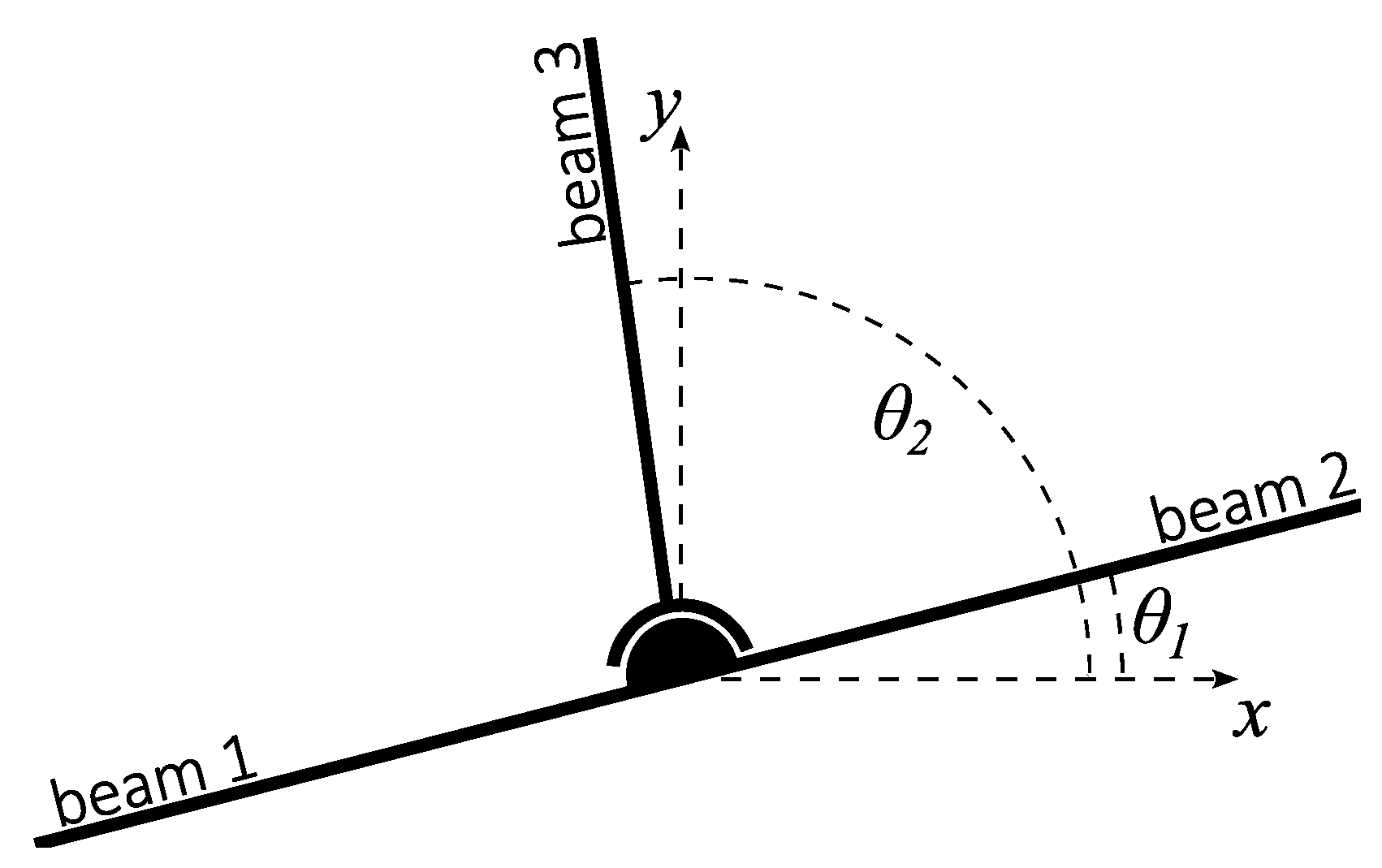
• The beams aggregated to the same rotational DOF remain rigidly connected, as in a typical frame node, with a full transmission of the bending moments between them (beams 1 and 2 in the example shown in Figure 1);
• In the unlocked (“off”) state of the node, the two rotational DOFs ${\theta }_1$ and ${\theta }_2$ remain uncoupled and rotate independently. The bending moments are not transmitted between the aggregated groups of adjacent beams (beams 1/2 and beam 3, respectively, in Figure 1);
• The locked (“on”) state of the node imposes (an approximation of) the following kinematic constraint:

  $${\dot{\theta }}_1={\dot{\theta }}_2,$$

  (1)

  which effectively couples the rotations of the two DOFs and allows the bending moments to be transmitted between all the adjacent beams.

Equation (1) is formulated in velocities instead of displacements/rotations. This allows the node to be locked in any relative rotation of the involved DOFs, without any preference for the initial equilibrium position.

Figure 1. Scheme of an example on/off controllable node.

Figure 1. Scheme of an example on/off controllable node.

2.2. Element Aggregation and the Viscous Coupling Matrix

In the process of building the global FE model of the entire structure, local matrices of the elements are first transformed into the global coordinate system and then aggregated to the global DOFs. For an on/off controllable node:

• All the local horizontal and vertical displacement DOFs of the adjacent beams are aggregated to the corresponding nodal displacements x or y.
• The local rotational DOFs of the beams are aggregated either to ${\theta }_1$ or to ${\theta }_2$, depending on the planned transmission of moments and operation of the node. For the example shown in Figure 1, the rotational DOFs of beams 1 and 2 are aggregated to ${\theta }_1$, while the rotational DOF of beam 3 is aggregated to ${\theta }_2$.

After the aggregation phase, the resulting global matrices represent the FE model of the global structure with all its controllable nodes in the “off” state (unlocked hinges or no transmission of moments). During a simulation of the dynamic structural response, the node can be switched to the “on” state (locked hinges, full transmission of moments) by coupling its rotational DOFs and imposing the kinematic constraint expressed in Equation (1). This is performed by means of an additional viscous damper of the relative rotation, which is modeled in the form of an additional damping matrix. In the local coordinate system $({\theta }_1,{\theta }_2)$, the damper matrix takes the following form:

$${\overline{\mathbf{C}}}_i=c_i\left[\begin{array}{cc}\phantom{-}1& -1\\ -1& \phantom{-}1\end{array}\right],$$

(2)

where i indexes the controllable nodes, and $c_i$ is a large coefficient. The matrix ${\overline{\mathbf{C}}}_i$ is then transformed to the global coordinates. In the “on” state, it is added to the global damping matrix in order to effectively block the relative rotation and simulate the coupling between the DOFs ${\theta }_1$ and ${\theta }_2$.

The described coupling technique is based on viscous damping, and thus it should be explicitly emphasized that it cannot be used for static analysis. However, in the case of dynamic analysis, it can be shown that such a viscous rotational damper reliably approximates a fully rigid connection with a single rotational DOF and a full transmission of moments [37].

2.3. Equation of Motion

The final equation of motion of the entire structure equipped with the controllable on/off nodes can be expressed in the following bilinear form:

$$\mathbf{M}\ddot{\mathbf{u}}\left(t\right)+\left(\mathbf{C}+\sum _i{\alpha }_i\left(t\right){\mathbf{C}}_i\right)\dot{\mathbf{u}}\left(t\right)+\mathbf{Ku}\left(t\right)=\mathbf{f}\left(t\right),$$

(3)

where $\mathbf{u}\left(t\right)$ is the vector of the generalized displacements, and the vector $\mathbf{f}\left(t\right)$ represents the external excitation force. The matrices $\mathbf{M}$, $\mathbf{C}$, and $\mathbf{K}$ denote, respectively, the global mass, damping, and stiffness matrices of the structure with all controllable nodes in the "off” state. Finally, the matrix ${\mathbf{C}}_i$ represents in the global coordinate system the rotational damper of the ith controllable node, which is activated and deactivated by means of the control function ${\alpha }_i\left(t\right)$,

$${\alpha }_i\left(t\right)\in \left\{0,1\right\}.$$

(4)

3. The Control Method

This section derives the proposed sliding mode control law. First, the control forces and the control aim are described. Then, the respective sliding mode control is proposed and formally stated in the form of the control law.

3.1. The Control Forces

Equation (3) represents the equation of motion. The terms with the control functions ${\alpha }_i\left(t\right)$ are moved to the right-hand side as

$$\mathbf{M}\ddot{\mathbf{u}}\left(t\right)+\mathbf{C}\dot{\mathbf{u}}\left(t\right)+\mathbf{Ku}\left(t\right)=\mathbf{f}\left(t\right)-\sum _i{\alpha }_i\left(t\right){\mathbf{C}}_i\dot{\mathbf{u}}\left(t\right),$$

(5)

where they become vectors of control forces that can be activated and deactivated in the on/off manner by means of the control functions ${\alpha }_i\left(t\right)\in \left\{0,1\right\}$. Due to the occurrence of the velocity term $\dot{\mathbf{u}}\left(t\right)$ on the right-hand side, the control forces are coupled to the structural response.

By introducing the modal coordinates $\mathit{\xi }\left(t\right)$,

$$\mathsf{\Phi }\mathit{\xi }\left(t\right)=\mathbf{u}\left(t\right),$$

(6)

where the matrix $\mathsf{\Phi }$ contains the modal vectors as columns, Equation (5) can be represented in the modal coordinates as follows:

$$\tilde{\mathbf{M}}\ddot{\mathit{\xi }}\left(t\right)+\tilde{\mathbf{C}}\dot{\mathit{\xi }}\left(t\right)+\tilde{\mathbf{K}}\mathit{\xi }\left(t\right)=\tilde{\mathbf{f}}\left(t\right)+\sum _i{\alpha }_i\left(t\right){\tilde{\mathbf{f}}}_i\left(t\right),$$

(7)

where

$${\tilde{\mathbf{f}}}_i\left(t\right)=-{\mathsf{\Phi }}^{\mathrm{T}}{\mathbf{C}}_i\mathsf{\Phi }\dot{\mathit{\xi }}\left(t\right)=-{\mathsf{\Phi }}^{\mathrm{T}}{\mathbf{C}}_i\dot{\mathbf{u}}\left(t\right).$$

(8)

As evident in Equation (8), in the “on” state of the ith controllable node the corresponding control force ${\tilde{\mathbf{f}}}_i\left(t\right)$ depends on and couples the modal responses. The modal matrices in Equation (7) take the following standard forms:

$$\begin{array}{cc}\hfill \tilde{\mathbf{M}}& ={\mathsf{\Phi }}^{\mathrm{T}}\mathbf{M}\mathsf{\Phi },\hfill \\ \hfill \tilde{\mathbf{C}}& ={\mathsf{\Phi }}^{\mathrm{T}}\mathbf{C}\mathsf{\Phi },\hfill \\ \hfill \tilde{\mathbf{K}}& ={\mathsf{\Phi }}^{\mathrm{T}}\mathbf{K}\mathsf{\Phi },\hfill \end{array}$$

(9a)

while the excitation force is

$$\tilde{\mathbf{f}}\left(t\right)={\mathsf{\Phi }}^{\mathrm{T}}\mathbf{f}\left(t\right).$$

(9b)

3.2. The Control Aim

The general control aim is to mitigate the vibrations in a selected DOF of the structure. Formally, it is defined in terms of the displacement in the selected DOF as follows:

$$u_k={\mathsf{\Phi }}_{k·}\mathit{\xi }=0,$$

(10)

where k represents the index of the selected DOF, and the column vector $\mathit{\xi }$ denotes a point in the modal coordinate space. The row vector ${\mathsf{\Phi }}_{k·}$ collects contributions from all the modal vectors in the kth DOF, and it is thus the kth row of the matrix $\mathsf{\Phi }$.

3.3. Sliding Mode Control

The control aim stated in Equation (10) defines a target hyperplane in the modal space. The general aim of the proposed control is to drive the current modal displacements toward this hyperplane. For each controllable node, its state in a time instant t is decided in dependence on the direction of the control forces, as the potentially activated control forces ${\tilde{\mathbf{f}}}_i\left(t\right)$ can point in the modal space toward or outward the target hyperplane. This can be determined as follows:

Let $\mathit{\xi }\left(t\right)$ be the structural displacement vector at time t expressed in modal coordinates, and $\Delta \mathit{\xi }\left(t\right)$ denotes the vector that points from point $\mathit{\xi }\left(t\right)$ to its perpendicular projection onto the hyperplane defined by Equation (10). Using standard linear algebra and the condition ${\mathsf{\Phi }}_{k·}\left(\mathit{\xi }\left(t\right)+\Delta \mathit{\xi }\left(t\right)\right)=0$, one can show that

$$\Delta \mathit{\xi }\left(t\right)=-{\mathsf{\Phi }}_{k·}\mathit{\xi }\left(t\right)\frac{{\mathsf{\Phi }}_{k·}^{\mathrm{T}}}{{\mathsf{\Phi }}_{k·}{\mathsf{\Phi }}_{k·}^{\mathrm{T}}}=-u_k\left(t\right)\frac{{\mathsf{\Phi }}_{k·}^{\mathrm{T}}}{{\mathsf{\Phi }}_{k·}{\mathsf{\Phi }}_{k·}^{\mathrm{T}}}.$$

(11)

If the control forces ${\tilde{\mathbf{f}}}_i\left(t\right)$ are activated, their direction (toward or outward the target hyperplane) can be determined according to the sign of the cosine between them and the vector $\Delta \mathit{\xi }\left(t\right)$. This means that the initial candidate for the control law can be stated as follows:

$${\alpha }_i\left(t\right)=H\left({\tilde{\mathbf{f}}}_i{\left(t\right)}^{\mathrm{T}}\Delta \mathit{\xi }\left(t\right)\right)=H\left(u_k\left(t\right){\mathsf{\Phi }}_{k·}{\mathsf{\Phi }}^{\mathrm{T}}{\mathbf{C}}_i\dot{\mathbf{u}}\left(t\right)\right),$$

(12)

where $H(·)$ is the Heaviside step function. According to Equation (12), a controllable node is switched to the "on” state if and only if the control forces thus activated point toward the target hyperplane. As described in the two following subsections, this initial control law is modified by

• Limiting the maximum switching frequency to avoid the chattering phenomenon;
• Introducing a phase-related correction.

3.4. Chattering Avoidance

The term chattering relates to very frequent switching of the control function. It is a harmful phenomenon that often occurs in systems with sliding mode control [38]. With the initial control law defined in Equation (12), the state switches of the ith controllable node, and thus also chattering, can occur either on the target hyperplane (when $u_k\left(t\right)=0$) or when the relative angular velocity of the potentially coupled rotational DOFs vanish (when ${\mathbf{C}}_i\dot{\mathbf{u}}\left(t\right)=0$). In this work, chattering is addressed in a simple way: For each controllable node, it is assumed that the switching time instants must be separated by a certain time interval of at least $\Delta t$. In other words, each switching action saturates the node and freezes its new state for the time interval of $\Delta t$. Such an assumption limits the effective maximum switching frequency and thus avoids chattering. In practice, the time interval $\Delta t$ will be related to the physical limitations of the actual actuator.

3.5. Phase-Related Correction and the Final Control Law

The phase-related optimum switching maps derived in [36], as well as similar maps obtained in [23] for the on/off skyhook control, suggest that the strict maximization of the restoring force might not always be the most effective approach to reduce vibrations. Therefore, the control forces determined according to Equation (12) are reversed when the current modal displacement $\mathit{\xi }\left(t\right)$ approaches the switching hyperplane. This is formalized as follows:

$${\alpha }_i\left(t\right)=\left\{\begin{array}{cc}1-H\left(u_k\left(t\right){\mathsf{\Phi }}_{k·}{\mathsf{\Phi }}^{\mathrm{T}}{\mathbf{C}}_i\dot{\mathbf{u}}\left(t\right)\right)\hfill & \mathrm{if}1\le \psi \left(t\right)\le 1+\kappa ,\hfill \\ H\left(u_k\left(t\right){\mathsf{\Phi }}_{k·}{\mathsf{\Phi }}^{\mathrm{T}}{\mathbf{C}}_i\dot{\mathbf{u}}\left(t\right)\right)\hfill & \mathrm{otherwise},\hfill \end{array}\right.$$

(13)

where $\psi \left(t\right)$ is related to the phase,

$$\psi \left(t\right)=\frac{arctan\left(u_k\left(t\right),{\dot{u}}_k\left(t\right)\right)}{\pi /2}\mathrm{mod}2,$$

(14)

and $\kappa \in (0,1)$ is a certain constant.

4. Numerical Experiment

The control method proposed in the previous section was tested in a numerical experiment of a shear-type structure subjected to random seismic excitation.

4.1. The Structure

In the numerical experiment, a FE model of a four-story shear structure was used, which is shown in Figure 2.

The geometric and material characteristics of the stories are similar to those used in [33]. The height and width of each story were 0.4 m. The cross-section of each beam was 8 mm × 10 mm. The Young modulus of the material was 210 GPa, and the density was 7860 kg/m³, which corresponds to steel. Eight controllable nodes, each of 1.2 kg mass, were placed at both ends of each horizontal beam.

The FE model of the structure had 32 non-fixed DOFs, i.e.,4 DOFs in each of the 8 controllable nodes, and 6 fixed DOFs in the 2 bottom fully supported nodes.

Table 1. Selected natural frequencies and damping ratios: for the structure shown in Figure 2 with all its controllable nodes in the “off” state and for the corresponding structure with all nodes rigid.

Mode No.	All Nodes “off” (Unlocked Hinges)		All Nodes Rigid
	Natural Freq. [Hz]	Damping Ratio [%]	Natural Freq. [Hz]	Damping Ratio [%]
1	0000.86	000.23	0003.76	001.00
2	0005.47	001.45	0011.97	003.18
3	0015.38	004.09	0021.49	005.72
4	0028.08	007.47	0030.44	008.09
5	0128.99	034.30	0134.38	035.73
…	…	…	…	…
24	0886.15	235.62	1666.34	443.06
…	…	…
30	1368.34	363.82

lists the natural frequencies and the modal damping ratios for the structure with the controllable nodes in the "off” state (unlocked hinges), as well as for the corresponding structure with the typical frame-like rigid nodes. The Rayleigh damping model was used, where the damping matrix is proportional to the stiffness matrix. The proportionality coefficient was selected in such a way that the first mode of the all-rigid structure had a damping ratio of 1%. The same proportionality coefficient was used for the structure with controllable nodes shown in Figure 2, which resulted in the damping ratio of the first mode being only 0.23%.

4.2. Excitation and Simulation Parameters

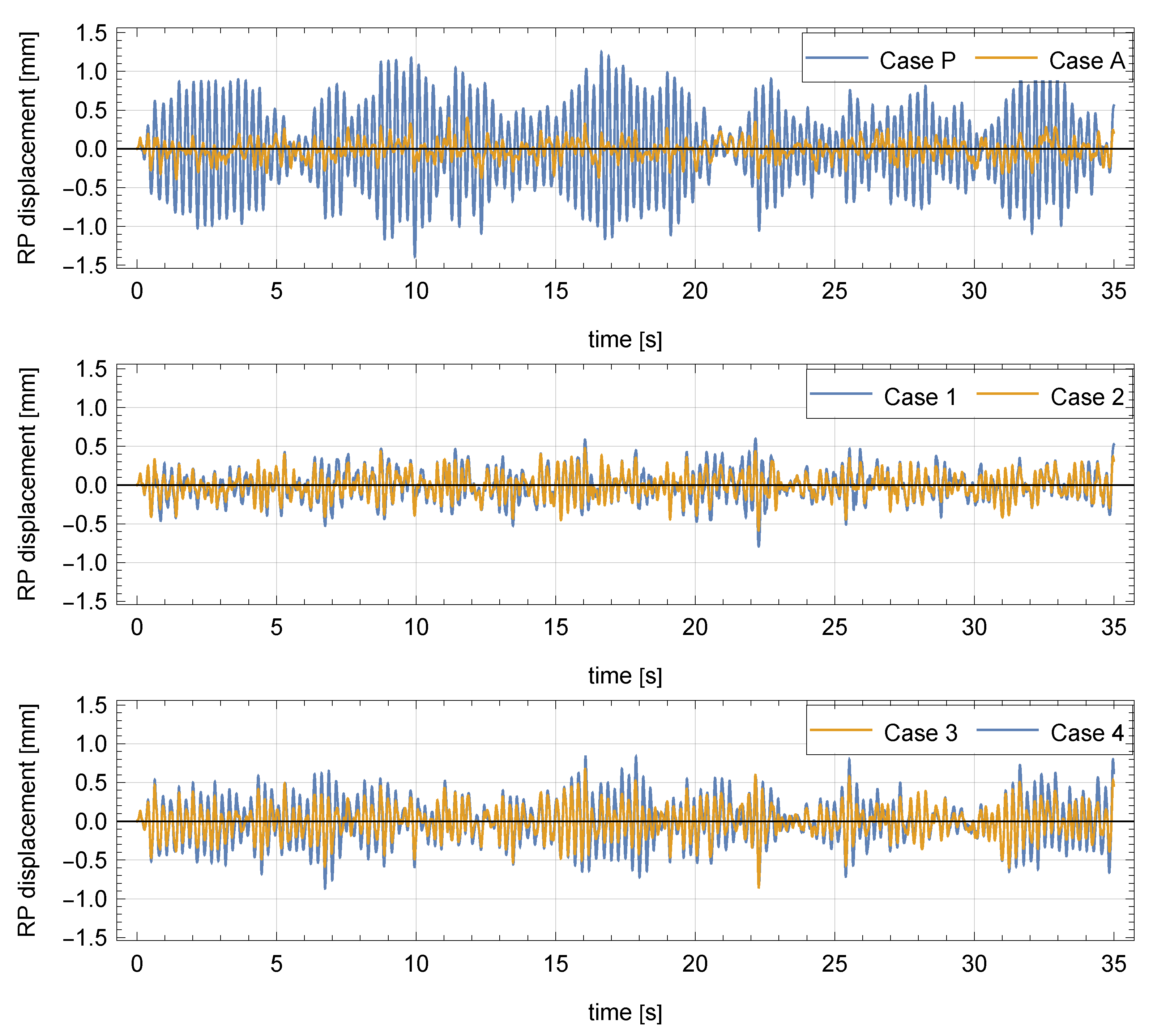
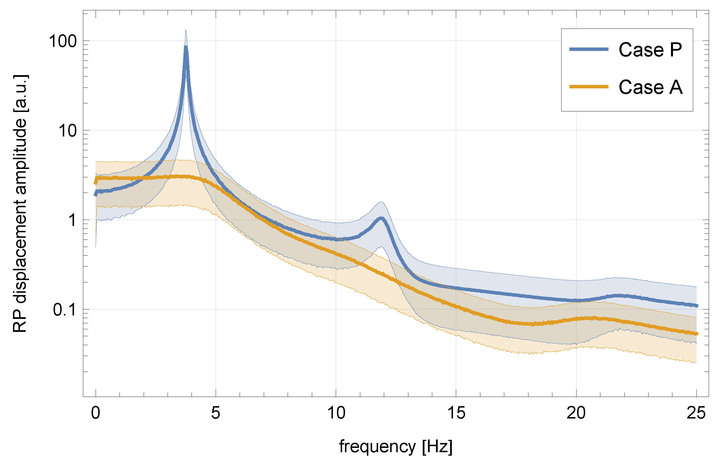
The structure is subjected to random seismic excitation. The excitation force $\mathbf{f}\left(t\right)$ in Equation (3) has thus the following form:

$$\mathbf{f}\left(t\right)=-\mathbf{M}{\ell }_{\mathrm{x}}a\left(t\right),$$

(15)

where $\mathbf{M}$ is the mass matrix of the entire structure, and ${\ell }_{\mathrm{x}}$ is a binary vector that selects all its horizontal DOFs. The ground acceleration is denoted by $a\left(t\right)$. In numerical simulations, the ground acceleration in each time step $t_j$ is modeled as an independent realization of a Gaussian random variable $N(0,1)$,

$$a\left(t_j\right)\sim N(0,1)\left[\frac{\mathrm{m}}{{\mathrm{s}}^2}\right].$$

(16)

The excitation is horizontal, and due to the symmetry of the structure, the controllable nodes are operated pairwise and synchronously using a single control function: Both nodes at each story are switched "on” and "off” simultaneously, so that they always remain in the same state. The initial state of the nodes is "on” (hinges locked), but in practice, it does not matter, as their state afterward is uniquely linked to the response.

The response is computed using zero initial conditions and the Newmark integration algorithm [39] with the typical values of its parameters ($\alpha =0.25$ and $\delta =0.5$), which guarantee unconditional stability and energy conservation [40]. The integration time step is 0.1 ms, which corresponds to about 6 time steps in a single period of the highest-frequency natural mode listed in Table 1.

The two parameters specific to the proposed control method are selected as follows: The constant $\kappa$ in Equation (13) (Section 3.5) is $\kappa =0.03$, and the saturation time interval for each controllable node is $\Delta t=5$ ms (Section 3.4), which corresponds to the maximum switching frequency of 100 Hz. The specific values of these two parameters are not crucial, which is verified in Section 4.3.

4.3. Results

The assumed seismic excitation is random white noise (see Equation (16)), and the computed response is correspondingly transient in the time domain. It is assumed that after 15 s, the response stabilizes in the probabilistic terms. All the analyses shown in this section are thus performed using 20 s long response data recorded in the time interval from 15 s to 35 s. At the time step of 0.1 ms, it corresponds to a total of 350,000 time steps per each full simulation.

The results were assessed quantitatively in terms of the root-mean-square (rms) time-domain response and the frequency-domain response (amplitude of the frequency response function (FRF)) at the reference point (RP) shown in Figure 2. As many as 4000 simulations were performed, each 35 s long, and the results are presented in terms of the distributions and/or the mean values and standard deviations. In total, six control cases were considered to compute, assess, and compare the responses. These control cases are listed in Table 2, and they can be summarized as follows:

• Passive structure (Case P in Table 2): This was the reference case. All the nodes remained in their "on” state throughout the entire simulation. This corresponded to a passive structure with typical rigid nodes and full transmission of moments;
• All stories controlled (Case A in Table 2): Nodes were controlled pairwise, independently, and synchronously for each of the four stories. There were four control functions: one function for each story;
• Single story controlled (Cases 1–4 in Table 2): The nodes of only a single story were controlled, while the other nodes remained in their "on” (rigid) state with the full transmission of moments. In each of these four cases, there was thus only one control function.

As an example, Figure 3, Figure 4 and Figure 5 present the results obtained for the same single random seismic excitation. Figure 3 plots the full-time-domain RP displacements computed for all the control cases and compares them with the RP displacements in the passive structure. For the purpose of the quantitative evaluations presented in the subsequent sections, the initial 15 s of each response is discarded. Figure 4 and Figure 5 plot the control functions in the initial 2 s for the fully controlled structure (Case A, Figure 4) and for all the single-story-controlled structures (Cases 1–4, Figure 5), together with the respective RP responses. The controllable nodes remained in the ”on" state 70–85% of the total simulation time, depending on the story and the control case. If necessary, the frequency of switching can be further controlled by the parameter $\Delta t$.

Table 2. Six control cases used to compute, assess, and compare the responses. The two nodes on each story were controlled pairwise and synchronously.

Case	No. of Control Functions	Remarks
P	0	Passive reference case. All nodes rigid
A	4	Each story controlled independently
1	1	Story No. 1 controlled. Other stories passive with rigid nodes
2	1	Story No. 2 controlled. Other stories passive with rigid nodes
3	1	Story No. 3 controlled. Other stories passive with rigid nodes
4	1	Story No. 4 controlled. Other stories passive with rigid nodes

Table 2. Six control cases used to compute, assess, and compare the responses. The two nodes on each story were controlled pairwise and synchronously.

Case	No. of Control Functions	Remarks
P	0	Passive reference case. All nodes rigid
A	4	Each story controlled independently
1	1	Story No. 1 controlled. Other stories passive with rigid nodes
2	1	Story No. 2 controlled. Other stories passive with rigid nodes
3	1	Story No. 3 controlled. Other stories passive with rigid nodes
4	1	Story No. 4 controlled. Other stories passive with rigid nodes

4.3.1. Root-Mean-Square Response

For each of the 4000 independently simulated white noise seismic excitations, the rms of the RP displacement was computed for the controlled structures (Cases A and 1–4) and then divided by the corresponding rms of the passive structure (Case P). The resulting rms reduction ratio can be treated as a measure of the effectiveness of the proposed control method.

The empirical probability density functions of the 4000 rms reduction ratios obtained this way are qualitatively presented in Figure 6 in the form of distribution plots. The corresponding means and standard deviations are listed in the second and third columns of Table 3. In all control cases, the proposed control method was able to significantly mitigate the displacements of the reference point. As expected, the best rms ratio was obtained when all the stories were controlled (Case A, rms reduced to 21.63%). However, the controllable nodes were effective even when placed at a single story only. In such a case, it was most advantageous to place them at the second story (Case 2, rms reduced to 29.12%), while the fourth story was the least advantageous location that, nevertheless, still provided considerable mitigation (Case 4, rms reduced to 51.60%).

4.3.2. Frequency-Domain Response

The displacement responses of the reference point (RP), obtained in all control cases and for all 4000 simulated random seismic excitations were also analyzed in the frequency domain. Figure 7 plots the mean amplitudes of the RP responses for the passive structure and the fully controlled structure (Cases P and A), together with their $\pm \sigma$ (one standard deviation) bands. In Figure 8, the mean response amplitudes obtained for all the considered control cases are compared.

Table 3. Control effectiveness for the five controlled structures, compared with the passive structure: means and standard deviations of the rms reduction ratios (see Figure 6), and mean amplitude reduction ratios at the first mode (see Figure 8).

Case	Rms Ratio		Mean Amplitude Ratio
	Mean [%]	Standard Deviation [%]	First Mode [%]
Case A	21.63	4.52	03.51
Case 1	36.84	7.25	11.89
Case 2	29.12	5.60	07.80
Case 3	37.05	7.02	14.49
Case 4	51.60	9.41	29.35

Table 3. Control effectiveness for the five controlled structures, compared with the passive structure: means and standard deviations of the rms reduction ratios (see Figure 6), and mean amplitude reduction ratios at the first mode (see Figure 8).

Case	Rms Ratio		Mean Amplitude Ratio
	Mean [%]	Standard Deviation [%]	First Mode [%]
Case A	21.63	4.52	03.51
Case 1	36.84	7.25	11.89
Case 2	29.12	5.60	07.80
Case 3	37.05	7.02	14.49
Case 4	51.60	9.41	29.35

The frequency interval of 0–25 Hz, shown in Figure 7 and Figure 8, includes the three fundamental natural frequencies of the structure (see Table 1). As expected, the dominant response component was always the first mode, while the amplitudes in the second and third modes were significantly smaller by one or two orders of magnitude. The control effectiveness could be thus assessed in terms of the reduction ratio of the mean amplitude in the crucial first natural mode. To this end, the peak mean amplitude of the first mode was divided by its peak mean amplitude in the passive structure. The resulting mean amplitude reduction ratios are listed in the last column of Table 3.

The fully controlled structure (Case A) provided the best broadband attenuation of vibrations: The first and the third amplitude peaks were significantly reduced, while the second peak completely disappeared. In fact, the peak amplitude in the first mode was significantly reduced in all the considered control cases, and even in the least effective Case 4, it was reduced by more than 70%.

Figure 8. Frequency-domain amplitudes of the RP displacement responses in all considered control cases (in arbitrary units, a.u.).

Figure 8. Frequency-domain amplitudes of the RP displacement responses in all considered control cases (in arbitrary units, a.u.).

The peak amplitudes in the second and third modes were considerably smaller and thus less important, but even they were reduced in most of the control cases. The exception was the second mode in Cases 1 and 4, as well as the third mode in Case 2. These small increases in the amplitude of the second and third modes were consistent with that of the intended global dissipation mechanisms provided by the on/off nodes: the transfer of the vibration energy toward higher-order modes, which are nonetheless highly damped by means of the natural mechanisms of material damping.

Finally, an important observation is the location of the peaks in the amplitude spectra of the RP displacements. As expected, and as attested by Table 1, the natural frequencies of the structure with the controllable nodes in the "off” state (unlocked hinges) were much lower than in the structure with its nodes in the rigid "on” state. The proposed control method intermittently switched the controllable nodes to their "off” state and thus decreased the global stiffness of the structure. Despite this decrease, as seen in Figure 7 and Figure 8, the reduced amplitude peaks largely maintained their original frequencies: there was no significant downward shift in the resonance frequencies.

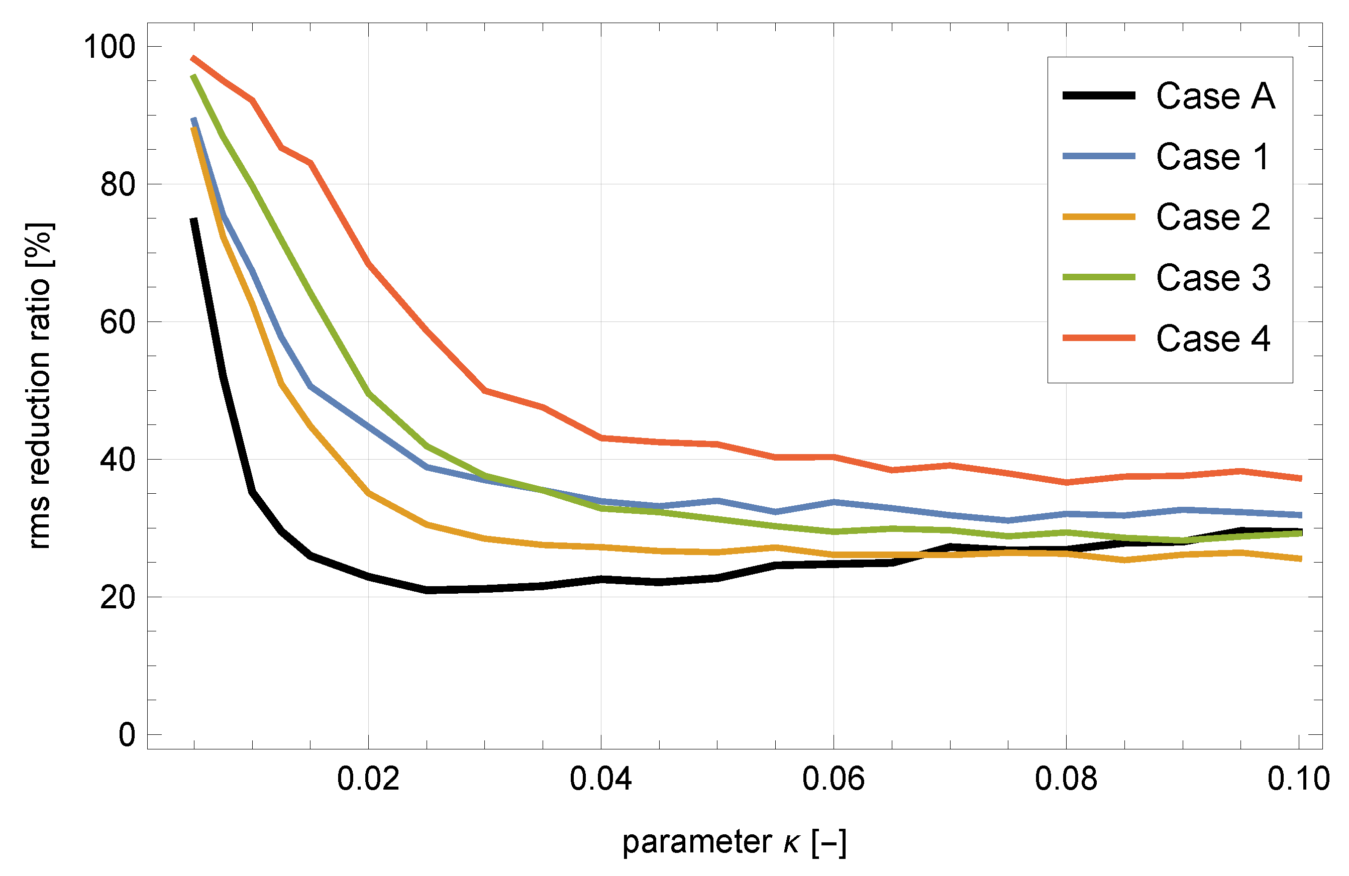
4.4. Sensitivity to Control Parameters

The proposed control method involves two control parameters that were determined on a trial-and-error basis. These are the phase-related constant $\kappa$ in Equation (13) and the node saturation time interval $\Delta t$, which is related to the maximum node switching frequency. Their specific values used in the simulations were $\kappa =0.03$ and $\Delta t=5$ ms.

The sensitivity of the results to these parameters was assessed in terms of the rms reduction ratio, computed for the time-domain RP displacements in all control cases. Figure 9 plots the dependence of the mean rms reduction ratio on the parameter $\kappa$ for $\Delta t=5$ ms. Similarly, Figure 10 plots the mean rms reduction ratio and shows its dependence on the parameter $\Delta t$ for $\kappa =0.03$. Each point in these plots is the mean value computed for 108 different realizations of the random seismic excitation. As seen in both figures, the effectiveness of the control remained relatively flat in a wide range of the considered parameters. Such a character of the plots confirms that the specific values of the parameters $\kappa$ and $\Delta t$ used here were not crucial.

5. Conclusions

This manuscript proposed a sliding mode control method intended for the semi-active damping of vibrations of frame-like structures. An untypical feature of the proposed method is that it is designed to be used with actuators of a specific type, namely on/off structural nodes that are capable of a controllable transmission of bending moments between selected adjacent beams. The control aim was formulated in terms of the displacements of a specific point of the structure. This contrasts with earlier research involving such nodes, which were formulated in general terms of the global structural energy and did not allow the mitigation effort to be explicitly focused on selected crucial areas of the structure.

The proposed method was verified in a numerical experiment of a four-story shear-type structure subjected to a repeated random seismic excitation. The on/off nodes were modeled using viscous rotational dampers. The control efficiency was assessed and confirmed in the time domain, in terms of the reduction ratio of the root-mean-square displacements, as well as in the frequency domain by investigating the response amplitude spectra and the peak reduction ratios. The obtained results were promising: Even a single pair of properly placed actuators allowed the rms response to be reduced by over 70%, while the amplitude peak at the dominant first natural mode of vibrations was reduced by over 92%. At the same time, the frequency shift of the remaining resonance peak was negligible. This confirmed that the global dynamic stiffness of the structure did not decrease in the crucial frequency range near the first natural frequency.

The research is ongoing, and the most imminent task is experimental verification in laboratory conditions, as well as the subsequent tests under real ground motion records. In further applications to larger-scale structures, the full state vector will not usually be available, and a possible solution in such a case is to use a reduced structural model and/or a state observer. Moreover, lab-scale actuators will have to be upscaled for such an application, which is a complex task in itself. A related research topic is also the development of a quantitative and numerically effective approach to the optimum placement of the actuators, where the aim needs to be expressed in terms of the local displacements instead of the global energy [41]. Another important research avenue is an application to modular structures, where the control design needs to take into account the interplay between the overall global structural dynamics and the module-level local dynamics [42].

References

1. Basu, B.; Bursi, O.S.; Casciati, F.; Casciati, S.; Del Grosso, A.E.; Domaneschi, M.; Faravelli, L.; Holnicki-Szulc, J.; Irschik, H.; Krommer, M.; et al. A European association for the control of structures joint perspective. Recent studies in civil structural control across Europe. Struct. Control Health Monit. 2014, 21, 1414–1436. [Google Scholar] [CrossRef]
2. Spencer, B., Jr.; Nagarajaiah, S. State of the art of structural control. J. Struct. Eng. 2003, 129, 845–856. [Google Scholar] [CrossRef]
3. Casciati, F.; Rodellar, J.; Yildirim, U. Active and semi-active control of structures-theory and applications: A review of recent advances. J. Intell. Mater. Syst. Struct. 2012, 23, 1181–1195. [Google Scholar] [CrossRef]
4. Saaed, T.E.; Nikolakopoulos, G.; Jonasson, J.E.; Hedlund, H. A state-of-the-art review of structural control systems. JVC/J. Vib. Control 2015, 21, 919–937. [Google Scholar] [CrossRef]
5. Parulekar, Y.; Reddy, G. Passive response control systems for seismic response reduction: A state-of-the-art review. Int. J. Struct. Stab. Dyn. 2009, 9, 151–177. [Google Scholar] [CrossRef]
6. Pawlak, Z.M.; Lewandowski, R. The effectiveness of the passive damping system combining the viscoelastic dampers and inerters. Int. J. Struct. Stab. Dyn. 2020, 20, 2050140. [Google Scholar] [CrossRef]
7. Huang, J.; Zhang, R.; Luo, Q.; Guo, X.; Cao, M. Study on optimal design of grotto–eave system with cable inerter viscous damper for vibration control. Buildings 2022, 12, 661. [Google Scholar] [CrossRef]
8. Dai, H.; Jing, X.; Wang, Y.; Yue, X.; Yuan, J. Post-capture vibration suppression of spacecraft via a bio-inspired isolation system. Mech. Syst. Signal Process. 2018, 105, 214–240. [Google Scholar] [CrossRef]
9. Warn, G.P.; Ryan, K.L. A review of seismic isolation for buildings: Historical development and research needs. Buildings 2012, 2, 300–325. [Google Scholar] [CrossRef] [Green Version]
10. Elias, S.; Matsagar, V. Research developments in vibration control of structures using passive tuned mass dampers. Annu. Rev. Control 2017, 44, 129–156. [Google Scholar] [CrossRef]
11. Lin, W.; Wang, A.; Chen, S.; Qi, A.; Su, Z. Structural vibration control with the implementation of a tuned mass rocking wall system. Buildings 2021, 11, 614. [Google Scholar] [CrossRef]
12. Karnopp, D. Active and semi-active vibration isolation. J. Vib. Acoust. Trans. ASME 1995, 117, 177–185. [Google Scholar] [CrossRef]
13. El Ouni, M.H.; Laissy, M.Y.; Ismaeil, M.; Kahla, N.B. Effect of shear walls on the active vibration control of buildings. Buildings 2018, 8, 164. [Google Scholar] [CrossRef] [Green Version]
14. Korkmaz, S. A review of active structural control: Challenges for engineering informatics. Comput. Struct. 2011, 89, 2113–2132. [Google Scholar] [CrossRef]
15. Shivashankar, P.; Gopalakrishnan, S. Review on the use of piezoelectric materials for active vibration, noise, and flow control. Smart Mater. Struct. 2020, 29, 053001. [Google Scholar] [CrossRef]
16. Sabatini, M.; Gasbarri, P.; Monti, R.; Palmerini, G.B. Vibration control of a flexible space manipulator during on orbit operations. Acta Astronaut. 2012, 73, 109–121. [Google Scholar] [CrossRef]
17. Symans, M.D.; Constantinou, M.C. Semi-active control systems for seismic protection of structures: A state-of-the-art review. Eng. Struct. 1999, 21, 469–487. [Google Scholar] [CrossRef]
18. Preumont, A. Vibration Control of Active Structures: An Introduction, 3rd ed.; Springer: Dordrecht, The Netherlands, 2011. [Google Scholar]
19. Garrido, H.; Curadelli, O.; Ambrosini, D. On the assumed inherent stability of semi-active control systems. Eng. Struct. 2018, 159, 286–298. [Google Scholar] [CrossRef]
20. Fisco, N.; Adeli, H. Smart structures: Part I — Active and semi-active control. Sci. Iran. 2011, 18, 275–284. [Google Scholar] [CrossRef] [Green Version]
21. Zhu, X.; Jing, X.; Cheng, L. Magnetorheological fluid dampers: A review on structure design and analysis. J. Intell. Mater. Syst. Struct. 2012, 23, 839–873. [Google Scholar] [CrossRef]
22. Kirk, D.E. Optimal Control Theory: An Introduction; Dover Publications: Mineola, NY, USA, 2004. [Google Scholar]
23. Potter, J.N.; Neild, S.A.; Wagg, D.J. Generalisation and optimisation of semi-active, on-off switching controllers for single degree-of-freedom systems. J. Sound Vib. 2010, 329, 2450–2462. [Google Scholar] [CrossRef] [Green Version]
24. Onoda, J.; Endo, T.; Tamaoki, H.; Watanabe, N. Vibration suppression by variable-stiffness members. AIAA J. 1991, 29, 977–983. [Google Scholar] [CrossRef]
25. Onoda, J.; Minesugi, K. Semiactive vibration suppression of truss structures by coulomb friction. J. Spacecr. Rocket. 1994, 31, 67–74. [Google Scholar] [CrossRef]
26. Ferri, A.A.; Heck, B.S. Analytical investigation of damping enhancement using active and passive structural joints. J. Guid. Control. Dyn. 1992, 15, 1258–1264. [Google Scholar] [CrossRef]
27. Gaul, L.; Lenz, J.; Sachau, D. Active damping of space structures by contact pressure control in joints. Mech. Struct. Mach. 1998, 26, 81–100. [Google Scholar] [CrossRef]
28. Gaul, L.; Nitsche, R. Friction control for vibration suppression. Mech. Syst. Signal Process. 2000, 14, 139–150. [Google Scholar] [CrossRef]
29. Gaul, L.; Nitsche, R. The role of friction in mechanical joints. Appl. Mech. Rev. 2001, 54, 93–106. [Google Scholar] [CrossRef]
30. Mróz, A.; Holnicki-Szulc, J.; Biczyk, J. Prestress Accumulation-Release Technique for Damping of Impact-Born Vibrations: Application to Self-Deployable Structures. Math. Probl. Eng. 2015, 2015. [Google Scholar] [CrossRef] [Green Version]
31. Poplawski, B.; Mikułowski, G.; Wiszowaty, R.; Jankowski, Ł. Mitigation of forced vibrations by semi-active control of local transfer of moments. Mech. Syst. Signal Process. 2021, 157, 107733. [Google Scholar] [CrossRef]
32. Mikułowski, G.; Poplawski, B.; Jankowski, Ł. Semi-active vibration control based on switchable transfer of bending moments: Study and experimental validation of control performance. Smart Mater. Struct. 2021, 30, 045005. [Google Scholar] [CrossRef]
33. Ostrowski, M.; Blachowski, B.; Poplawski, B.; Pisarski, D.; Mikulowski, G.; Jankowski, L. Semi-active modal control of structures with lockable joints: General methodology and applications. Struct. Control Health Monit. 2021, 28, e2710. [Google Scholar] [CrossRef]
34. Orlowska, A.; Galezia, A.; Swiercz, A.; Jankowski, L. Mitigation of vibrations in sandwich-type structures by a controllable constrained layer. JVC/J. Vib. Control 2021, 27, 1595–1605. [Google Scholar] [CrossRef]
35. Young, K.D.; Utkin, V.I.; Özgüner, Ü. A control engineer’s guide to sliding mode control. IEEE Trans. Control Syst. Technol. 1999, 7, 328–342. [Google Scholar] [CrossRef] [Green Version]
36. Michajłow, M.; Jankowski, Ł.; Szolc, T.; Konowrocki, R. Semi-active reduction of vibrations in the mechanical system driven by an electric motor. Optim. Control Appl. Methods 2017, 38, 922–933. [Google Scholar] [CrossRef]
37. Poplawski, B.; Mikułowski, G.; Mróz, A.; Jankowski, Ł. Decentralized semi-active damping of free structural vibrations by means of structural nodes with an on/off ability to transmit moments. Mech. Syst. Signal Process. 2018, 100, 926–939. [Google Scholar] [CrossRef]
38. Lee, H.; Utkin, V.I. Chattering suppression methods in sliding mode control systems. Annu. Rev. Control 2007, 31, 179–188. [Google Scholar] [CrossRef]
39. Bathe, K.J. Finite Element Procedures, 2nd ed.; Pearson College Div: Victoria, BC, Canada, 2014. [Google Scholar]
40. Krenk, S. Energy conservation in Newmark based time integration algorithms. Comput. Methods Appl. Mech. Eng. 2006, 195, 6110–6124. [Google Scholar] [CrossRef]
41. Poplawski, B.; Mikułowski, G.; Pisarski, D.; Wiszowaty, R.; Jankowski, Ł. Optimum actuator placement for damping of vibrations using the Prestress-Accumulation Release control approach. Smart Struct. Syst. 2019, 24, 27–35. [Google Scholar] [CrossRef]
42. Zawidzki, M.; Jankowski, Ł. Multiobjective optimization of modular structures: Weight versus geometric versatility in a Truss-Z system. Comput.-Aided Civ. Infrastruct. Eng. 2019, 34, 1026–1040. [Google Scholar] [CrossRef]
Figure 2. The four-story shear structure used for numerical verification. The control aim is to mitigate horizontal displacements of the reference point (RP) under random seismic excitation.
Buildings 13 00348 g002
Figure 3. Example displacements of the reference point for the passive and fully controlled structures (Case P and Case A, top plot); the first- and second-story-controlled structures (Case 1 and Case 2, middle plot); and the third- and fourth-story-controlled structures (Case 3 and Case 4, bottom plot). All plots used vertical axes of the same range.
Buildings 13 00348 g003
Figure 4. Control functions of the four stories for the fully controlled structure together with the corresponding RP displacement (Case A) and the reference RP displacement in the passive structure (Case P).
Buildings 13 00348 g004
Figure 5. Control functions for the single controlled story structures together with the corresponding RP displacements (Cases 1–4) and the reference RP displacement in the passive structure (Case P).
Buildings 13 00348 g005
Figure 6. Distribution plots (qualitative representations of the empirical probability density functions) of the rms reduction ratios for the five controlled structures.
Buildings 13 00348 g006
Figure 7. Frequency-domain amplitudes of the RP displacement responses together with their ± σ bands for the passive and fully controlled structures (in arbitrary units, a.u.).
Buildings 13 00348 g007
Figure 9. Dependence of the rms reduction ratio on the parameter κ for Δ t = 5 ms in all control cases. Mean values were computed for 108 different random seismic excitations.
Buildings 13 00348 g009
Figure 10. Dependence of the rms reduction ratio on the parameter Δ t for κ = 0.03 in all control cases. Mean values were computed for 108 different random seismic excitations.
Buildings 13 00348 g010