Optimal Cluster Scheduling of Active–Reactive Power for Distribution Network Considering Aggregated Flexibility of Heterogeneous Building-Integrated DERs

Abstract

This paper proposes an active–reactive power collaborative scheduling model with cluster division for the flexible distributed energy resources (DERs) of smart-building systems to resolve the high complexity of the centralized optimal scheduling of massive dispersed DERs in the distribution network. Specifically, the optimization objective of each cluster is to minimize the operational cost, the power-loss cost, and the penalty cost for flexibility deficiency, and the second-order cone-based branch flow method is utilized to convert the power-flow equations into linearized cone constraints, reducing the nonlinearity and heavy computation burden of the scheduling model. Customized virtual battery models for building-integrated flexible DERs are developed to aggregate the power characteristics of flexible resources while quantifying their regulation capacities with time-shifting power and energy boundaries. Moreover, a cluster division algorithm considering the module degree index based on the electrical distance and the flexible balance contribution index is formulated for cluster division to achieve information exchange and energy interaction in the distribution network with a high proportion of building-integrated flexible DERs. Comparative studies have demonstrated the superior performance of the proposed methodology in economic merits and voltage regulation.

1. Introduction

1.1. Relevant Background

The construction sector is the third-largest energy consumer, accounting for 33% of global energy demand and 16% of global CO₂ emissions in 2022 [1]. Considering the growing tendency of urbanization progress and the continuous development of the power industry, the proportion of construction energy consumption is expected to increase by 40% in 2030 and even 50% in 2050 [2]. The aggregation of flexible DERs in buildings is recognized as a promising alternative method to reduce CO₂ emissions and energy consumption, promoting the profound integration of distributed energy resources (DERs) and building energy supply [3]. Smart-building systems equipped with power-access points could achieve flexible resource aggregation and exploit the regulation capacity of these resources sufficiently, intensifying the interdependency between buildings and electricity networks [3,4]. Nevertheless, the location of building-integrated photovoltaics (BIPVs), building-integrated electric vehicles (BIEVs), building-integrated energy storage (BIES), building-integrated temperature-controlled load (BITC), and other types of comprehensive energy production and storage equipment in smart-building systems are generally scattered, resulting in the high complexity of centralized optimization scheduling due to the lack of information exchange and energy interaction [4,5,6]. Consequently, the optimization scheduling of a distribution network with cluster division for flexible resources integrated into smart-building systems would be ideal for the high-penetrated deployment of DERs to meet carbon-neutral targets.

One typical method studied in [7] for cluster optimization scheduling is to use the second-order neighborhood similarity matrix and modular matrix to extract relatively more comprehensive complex network feature information for network division. Another example is a chromosome-encoding method considering the modular index based on the electrical design to satisfy the demand of distribution network programmers [8]. In further research, a K-means clustering algorithm based on the variation sensitivity of voltage to power between nodes to solve the voltage overlimit and voltage fluctuations is used [9]. Moreover, to tackle difficulties in uncertainty and centralized control, a multi-time rolling dynamic cluster division method with the equilibrium degree of reactive power for active distribution networks was developed [10]. However, the cluster division in these studies only involves a single index without considering comprehensive indexes, including flexibility regulation capacity and electrical connection. In addition, the active–reactive power collaborative optimization scheduling of distribution networks is acknowledged as an effective strategy for handling the uncertainties from dispersive DERs. A method for the coordinated optimal operation scheduling of active distribution networks was developed to meet the electricity demand of the building itself with interconnected electric vehicles and integrated RESs [11]. To implement optimal power dispatch and significantly reduce the overall operation cost of the microgrid, a method for optimal energy and power management of microgrids consisting of mega buildings, plug-in electric vehicles (PEVs), and renewable energy sources (RESs) was designed [12]. Furthermore, an energy management system (EMS) for microgrids of building prosumers based on a hierarchical multi-agent system (MAS) was studied in [13] to minimize the operation cost of a microgrid, considering many operation and technical constraints.

Integration and quantification for the regulation capacity of flexible resources are regarded as effective means to take advantage of the flexibility of smart-building systems [4,14,15,16,17,18]. Several important investigations have been reported on the virtual battery model [14], virtual synchronous machine model [15], flexible supply-and-demand balance model [16], and node power model [17] for the aggregation of flexible resources. A generic and scalable approach considering zonotopic sets for flexible energy systems was studied in [18] to describe their flexibility quantitatively. The authors use a constraint space-superposition method based on Minkowski Sum to seek the maximal inner cube constraints for the virtual synchronous machine of a heat pump cluster [19]. Moreover, the authors in [20] developed a day-ahead optimal scheduling model based on the generalized virtual battery model to determine the energy schedule and reserve capacity of electric vehicles and air conditioning. Additionally, a flexibility assessment can represent the abundance of flexible resources in a distribution network and has been comprehensively investigated with the insufficient ramping resource expectation index [21], the network flexibility index [22], the technical uncertain scenario flexibility index [23], and the technical–economic uncertainty scenario flexibility index [24]. A quantitative assessment method for power system flexibility based on probabilistic optimal power flow was developed to improve system flexibility and operating economy [21,22]. The authors in [23] studied a new distribution system flexibility evaluation method based on cloud models to address the difficulty in fully characterizing the flexibility status of a system. Furthermore, to quantify the transmission capacity of power grids and effectively improve the flexibility of power systems, an evaluation method of supply-and-demand balance considering flexible carrying capacity was studied in [24]. However, the comprehensive effect of the indexes on the flexibility state of the system is usually neglected in these studies.

Aggregation techniques, such as the k-order approximate model [25], the multi-time-scale approximate model [26], the real-time aggregation flexibility feedback method [27], and the Minkowski Sum [19] have been exploited to simplify the constraints of the aggregation feasible domains and realize the flexibility of the system. The authors studied a virtual power plant aggregation and operation mechanism to effectively guarantee the stability of the aggregation results [14]. An adaptive and robust optimization algorithm was adopted to accurately quantify the maximum power support range of the heat grid to the power grid [17]. After the aggregation of the flexible resources, the coordination and optimization of the distribution network with cluster division based on the flexible resources in the smart-building system can be achieved. Nevertheless, the potential active and reactive power support capacitates from the clusters of building-integrated flexible DERs for distribution networks are not involved.

1.2. Contribution

In this paper, an active–reactive power collaborative scheduling model with cluster division is proposed for the flexible DERs of smart-building systems to resolve the high complexity of centralized optimal scheduling for massively dispersed DERs in the distribution network. The detailed contributions of this paper are summarized as follows:

• The customized virtual battery models are developed for building-integrated flexible DERs to aggregate the power characteristics while quantifying the operation and regulation capacity with the time-shifting energy state, the energy boundary, and the power boundary. A constrained space-superposition method with Minkowski Sum is exploited to derive the summation of the regulation capacity of building-integrated flexible DERs.
• A cluster division algorithm considering the structural and functional cluster division indexes for the building-integrated flexible DERs is proposed to automatically divide the distribution network with a high proportion of renewable energy and flexible DERs into the optimal clusters. The structural cluster division index refers to the module degree index based on the electrical distance, which can ensure the close electrical connection of the nodes within the clusters, and the functional cluster division index represents the flexible balance contribution index, measuring the matching degree between the distributed power consumption demands and the supply of building-integrated flexible DERs.
• An optimal active–reactive power collaborative scheduling model for the clusters of building-integrated flexible DERs is formulated to minimize the operational cost, the power-loss cost, and the penalty cost for flexibility deficiency, in which the second-order cone-based branch flow method is exploited to decompose the nonlinearity and nonconvexity of the power-flow equation and the nodal voltage magnitude constraint into the linearized cone model by introducing the intermediate variable.

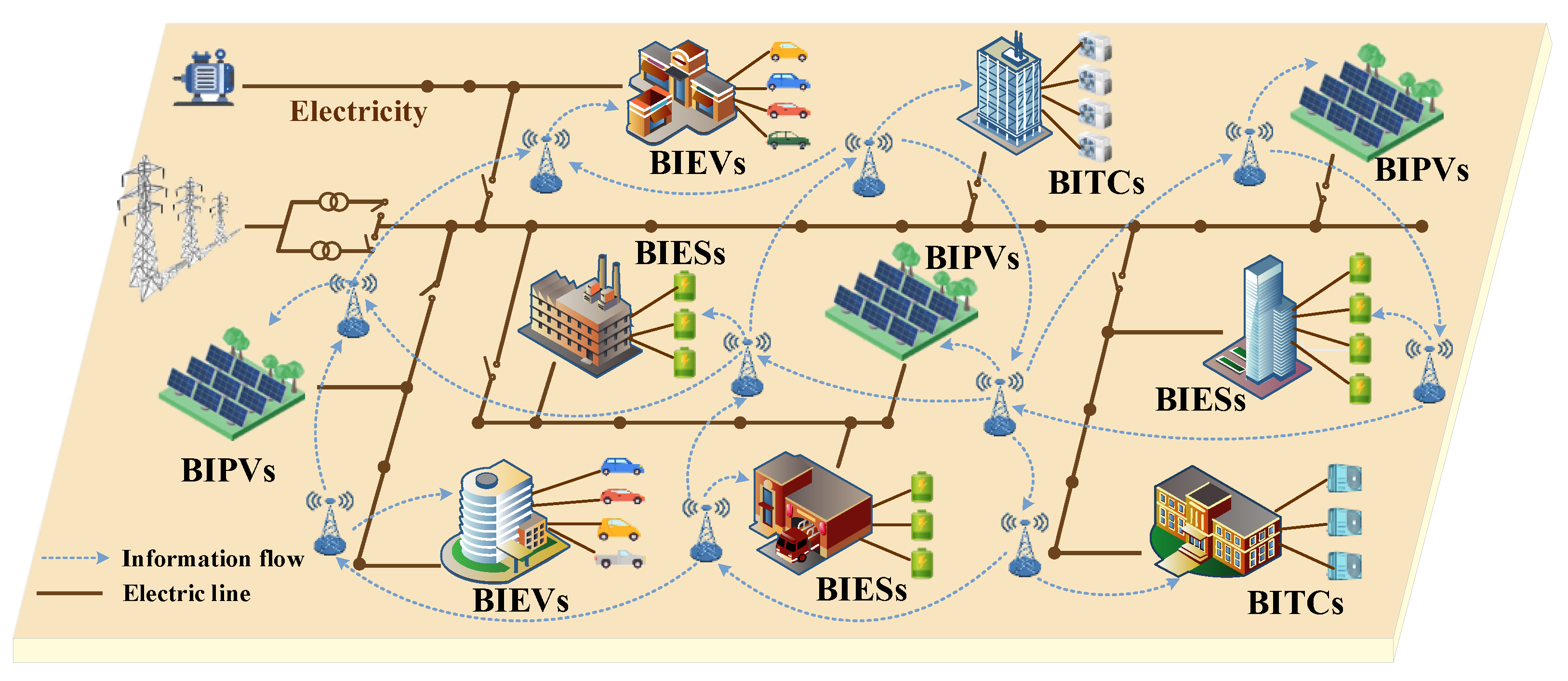
2. Flexible Regulation Capacity of Flexible DERs in a Smart-Building System

2.1. Smart-Building System

Figure 1 depicts the typical modality of a smart-building system among a highly renewable-penetrated distribution network. The smart-building system is generally equipped with cogeneration systems, distributed photovoltaics, electric vehicles, heat pumps, and energy storage to satisfy the demand for electricity and the cold and heat load in the building [5]. To fully utilize the space and time flexibility of building-integrated flexible DERs, the establishment of a virtual battery model for flexible DERs is necessary, which can quantify and integrate the flexibility and regulation capacity of these resources.

2.2. Battery Model of ES in a Smart-Building System

BIES can transfer the electricity generated by BIPVs to balance the energy of the power system, improving the reliability of system operation and power supply quality. A battery model of ES in a smart-building system (1), consisting of charge power constraints, discharge power constraints, and energy state constraints, is developed to describe the operating characteristic mathematically:

$$P_{\mathrm{ch},i,t,\min }^{\mathrm{ES}}\le P_{\mathrm{ch},i,t}^{\mathrm{ES}}\le P_{\mathrm{ch},i,t,\max }^{\mathrm{ES}}$$

(1a)

$$P_{\mathrm{dis},i,t,\min }^{\mathrm{ES}}\le P_{\mathrm{dis},i,t}^{\mathrm{ES}}\le P_{\mathrm{dis},i,t,\max }^{\mathrm{ES}}$$

(1b)

$$E_{i,t,\min }^{\mathrm{ES}}\le E_{i,t}^{\mathrm{ES}}\le E_{i,t,\max }^{\mathrm{ES}}$$

(1c)

$$E_{i,t+1}^{\mathrm{ES}}=E_{i,t}^{\mathrm{ES}}+P_{i,t}^{\mathrm{ES}}\Delta t=E_{i,t}^{\mathrm{ES}}+\left({\eta }_{\mathrm{ch}}^{\mathrm{ES}}{P}_{\mathrm{ch},i,t}^{\mathrm{ES}}-\frac{P_{\mathrm{dis},i,t}^{\mathrm{ES}}}{{\eta }_{\mathrm{dis}}^{\mathrm{ES}}}\right)\Delta t$$

(1d)

where $P_{\mathrm{c}\mathrm{h},i,t}^{\mathrm{E}\mathrm{S}}$and $P_{\mathrm{d}\mathrm{i}\mathrm{s},i,t}^{\mathrm{E}\mathrm{S}}$ are the charging and discharging power of BIES connected at node $i$ and time $t$; $P_{\mathrm{c}\mathrm{h},i,t,\mathrm{m}\mathrm{i}\mathrm{n}}^{\mathrm{E}\mathrm{S}}$, $P_{\mathrm{c}\mathrm{h},i,t,\mathrm{m}\mathrm{a}\mathrm{x}}^{\mathrm{E}\mathrm{S}}$, $P_{\mathrm{d}\mathrm{i}\mathrm{s},i,t,\mathrm{m}\mathrm{i}\mathrm{n}}^{\mathrm{E}\mathrm{S}}$, and $P_{\mathrm{d}\mathrm{i}\mathrm{s},i,t,\mathrm{m}\mathrm{a}\mathrm{x}}^{\mathrm{E}\mathrm{S}}$ denote the lower and upper bounds of the charging and discharging power of BIES; $E_{i,t}^{\mathrm{E}\mathrm{S}}$and $P_{i,t}^{\mathrm{E}\mathrm{S}}$ are the operation capacity and the actual power of BIES; $E_{i,t,\mathrm{m}\mathrm{a}\mathrm{x}}^{\mathrm{E}\mathrm{S}}$ and $E_{i,t,\mathrm{m}\mathrm{i}\mathrm{m}}^{\mathrm{E}\mathrm{S}}$ are the threshold of the operation capacity of BIES; ${\eta }_{\mathrm{c}\mathrm{h}}^{\mathrm{E}\mathrm{S}}$ and ${\eta }_{\mathrm{d}\mathrm{i}\mathrm{s}}^{\mathrm{E}\mathrm{S}}$ are the charge and discharge efficiency coefficients of BIES, and $∆t$ is the time interval.

The flexible regulation capacity of ES in smart-building systems with energy time-shift capacity and power regulation capacity can be expressed as

$$F_{i,t}^{\mathrm{ES},\sup ,\mathrm{up}}=P_{i,t,\max }^{\mathrm{ES}}-P_{i,t}^{\mathrm{ES}}$$

(2a)

$$F_{i,t}^{\mathrm{ES},\sup ,\mathrm{dn}}=P_{i,t}^{\mathrm{ES}}-P_{i,t,\min }^{\mathrm{ES}}$$

(2b)

where $F_{i,t}^{\mathrm{E}\mathrm{S},\mathrm{s}\mathrm{u}\mathrm{p},\mathrm{u}\mathrm{p}}$ and $F_{i,t}^{\mathrm{E}\mathrm{S},\mathrm{s}\mathrm{u}\mathrm{p},\mathrm{d}\mathrm{n}}$ denote the upgraded flexible energy supply and the downgraded flexible energy supply of BIES connected at node $i$ and time $t$, deriving from the lower and upper bounds of the actual power $P_{i,t,\mathrm{m}\mathrm{i}\mathrm{n}}^{\mathrm{E}\mathrm{S}}$ and $P_{i,t,\mathrm{m}\mathrm{a}\mathrm{x}}^{\mathrm{E}\mathrm{S}}$ of BIES.

2.3. Virtual Battery (VB) Model in a Smart-Building System

The VB model can accurately describe the operation and regulation characteristics of flexible DERs by constraining energy state, energy boundary, and power boundary, which can be expressed as

$$P_{i,t,\min }^G\le P_{i,t}^G\le P_{i,t,\max }^G$$

(3a)

$$E_{i,t,\min }^G\le E_{i,t}^G\le E_{i,t,\max }^G$$

(3b)

$$E_{i,t+1}^G=E_{i,t}^G+P_{i,t}^G\Delta t+\Delta E_{i,t}^G$$

(3c)

where $P_{i,t}^G$ and $E_{i,t}^G$ are the regulation power and the flexibility reserve energy of flexible DERs in a smart-building system connected at node $i$ and time $t$; $P_{i,t,\mathrm{m}\mathrm{i}\mathrm{n}}^G$, $P_{i,t,\mathrm{m}\mathrm{a}\mathrm{x}}^G$, $E_{i,t,\mathrm{m}\mathrm{i}\mathrm{n}}^G$, and $E_{i,t,\mathrm{m}\mathrm{a}\mathrm{x}}^G$ denote the lower and upper bounds of the regulation power and the flexibility reserve energy; (3c) represents the state of the flexibility reserve energy for the flexible DERs, and $∆E_{i,t}^G$ is the effect of other factors on the electric energy of the VB model.

2.4. VB Model of EV in a Smart-Building System

In general, the power battery of BIEV can achieve power interaction with the grid through flexibly switching between charging, placing, and discharging states. The grid-connected operation status of BIEV is illustrated in Figure 2, where BIEV with an initial operating capacity of $E_{i,t_0}^{\mathrm{E}\mathrm{V}}$ are connected to the grid with the maximum charge and discharge power of $P_{\mathrm{c}\mathrm{h},i,t,\mathrm{m}\mathrm{a}\mathrm{x}}^{\mathrm{E}\mathrm{V}}$and$P_{\mathrm{d}\mathrm{i}\mathrm{s},i,t,\mathrm{m}\mathrm{a}\mathrm{x}}^{\mathrm{E}\mathrm{V}}$ at time $t_0$, reaching the expected operating capacity of $E_{i,t}^{\mathrm{E}\mathrm{V}}$ when off the grid at time $t_1$.

Thus, the virtual battery model of BIEV can be formulated as follows:

$$P_{\mathrm{ch},i,t,\min }^{\mathrm{EV}}\le P_{\mathrm{ch},i,t}^{\mathrm{EV}}\le P_{\mathrm{ch},i,t,\max }^{\mathrm{EV}}$$

(4a)

$$P_{\mathrm{di}s,i,t,\min }^{\mathrm{EV}}\le P_{\mathrm{di}s,i,t}^{\mathrm{EV}}\le P_{\mathrm{di}s,i,t,\max }^{\mathrm{EV}}$$

(4b)

$$E_{i,t_0}^{\mathrm{EV}}-P_{\mathrm{dis},i,t,\max }^{\mathrm{EV}}(t-t_0)\le E_{i,t}^{\mathrm{EV}}\le E_{i,t_0}^{\mathrm{EV}}+P_{\mathrm{ch},i,t,\max }^{\mathrm{EV}}(t-t_0)$$

(4c)

$$E_{i,t+1}^{\mathrm{EV}}=E_{i,t}^{\mathrm{EV}}+P_{i,t}^{\mathrm{EV}}\Delta t=E_{i,t}^{\mathrm{EV}}+\left({\eta }_{\mathrm{ch}}^{\mathrm{EV}}{P}_{\mathrm{ch},i,t}^{\mathrm{EV}}-\frac{P_{\mathrm{dis},i,t}^{\mathrm{EV}}}{{\eta }_{\mathrm{dis}}^{\mathrm{EV}}}\right)\Delta t$$

(4d)

where $P_{\mathrm{c}\mathrm{h},i,t,\mathrm{m}\mathrm{i}\mathrm{n}}^{\mathrm{E}\mathrm{V}}$ and $P_{\mathrm{d}\mathrm{i}\mathrm{s},i,t,\mathrm{m}\mathrm{i}\mathrm{n}}^{\mathrm{E}\mathrm{V}}$ are the minimum thresholds of the charging and discharging power of BIEV connected at node $i$ and time $t$; $P_{\mathrm{c}\mathrm{h},i,t}^{\mathrm{E}\mathrm{V}}$, $P_{\mathrm{d}\mathrm{i}\mathrm{s},i,t}^{\mathrm{E}\mathrm{V}}$, $P_{i,t}^{\mathrm{E}\mathrm{V}}$, and $E_{i,t}^{\mathrm{E}\mathrm{V}}$ denote the charging power, discharging power, actual power, and operation capacity; ${\eta }_{\mathrm{c}\mathrm{h}}^{\mathrm{E}\mathrm{V}}$ and ${\eta }_{\mathrm{d}\mathrm{i}\mathrm{s}}^{\mathrm{E}\mathrm{V}}$ are the charge and discharge efficiency coefficients of BIEV. (4c) and (4d) represent the boundary of operation capacity and the operation state.

Then, considering that the power boundary $P_{i,t,\mathrm{m}\mathrm{a}\mathrm{x}}^{\mathrm{E}\mathrm{V}}$ and $P_{i,t,\mathrm{m}\mathrm{i}\mathrm{n}}^{\mathrm{E}\mathrm{V}}$of BIEV are affected by the operation capacity, the upgraded flexible energy supply $F_{i,t}^{\mathrm{E}\mathrm{V},\mathrm{s}\mathrm{u}\mathrm{p},\mathrm{u}\mathrm{p}}$ and the downgraded flexible energy supply $F_{i,t}^{\mathrm{E}\mathrm{V},\mathrm{s}\mathrm{u}\mathrm{p},\mathrm{d}\mathrm{n}}$ of EV in a smart-building system can be expressed as

$$F_{i,t}^{\mathrm{EV},\sup ,\mathrm{up}}=\min \{P_{i,t,\max }^{\mathrm{EV}}-P_{i,t}^{\mathrm{EV}},\frac{E_{i,t,\max }^{\mathrm{EV}}-E_{i,t}^{\mathrm{EV}}}{\Delta t}\}$$

(5a)

$$F_{i,t}^{\mathrm{EV},\sup ,\mathrm{dn}}=\min \{P_{i,t}^{\mathrm{EV}}-P_{i,t,\min }^{\mathrm{EV}}P,\frac{E_{i,t}^{\mathrm{EV}}-E_{i,t,\min }^{\mathrm{EV}}}{\Delta t}\}$$

(5b)

2.5. VB Model of TCL in a Smart-Building System

The equivalent thermal parameter model is adopted to describe the thermal dynamics characteristics of TCL, which equates the internal environment, external environment, and heating (cooling) capacity to circuit devices to analyze the dynamic change relationship of the indoor temperature and power [28,29]. As illustrated in Figure 3, the heating capacity $Q_{i,t}^1$ of the temperature control load can be defined as the sum of the heat absorbed by the room $Q_{i,t}^2$and the air convection heat $Q_{i,t}^3$.

(1d) shows that the energy of the BIES is equal to the superposition of the energy in the past state, the storage energy, and the release energy in the current state. Similarly, the indoor temperature $T_{\mathrm{i}\mathrm{n},i,t}^{\mathrm{T}\mathrm{C}\mathrm{L}}$ of the TCL is equal to the summation of the indoor temperature in the past state, warming, and cooling in the current state. When ambient temperature $T_{\mathrm{o}\mathrm{u}\mathrm{t},i,t}^{\mathrm{T}\mathrm{C}\mathrm{L}}$ is higher than indoor temperature, the temperature of the heating equipment $T_{\mathrm{h}\mathrm{e}\mathrm{a}\mathrm{t},i,t}^{\mathrm{T}\mathrm{C}\mathrm{L}}$ and the ambient temperature together transfers the heat quantity from high temperature to low temperature, increasing indoor temperature and the energy of the VB model. On the contrary, when the indoor temperature is higher in the summer, the cooling capacity of TCL works to reduce the indoor temperature, which is equivalent to the decrease in the energy of the VB model, as follows:

$$\{\begin{array}{l}{Q}_{i,t}^1=Q_{i,t}^2+Q_{i,t}^3\\ Q_{i,t}^1=A_1{\eta }^{\mathrm{TCL}}(T_{\mathrm{heat},i,t}^{\mathrm{TCL}}-T_{\mathrm{in},i,t}^{\mathrm{TCL}})\\ Q_{i,t}^2=\rho \mathrm{c}V(T_{\mathrm{in},i,t+1}^{\mathrm{TCL}}-T_{\mathrm{in},i,t}^{\mathrm{TCL}})\\ Q_{i,t}^3=A_2{\eta }^{\mathrm{Wall}}(T_{\mathrm{in},i,t}^{\mathrm{TCL}}-T_{\mathrm{out},i,t}^{\mathrm{TCL}})\\ {\eta }^{\mathrm{COP}}=\frac{P_{i,t}^{\mathrm{TCL}}\Delta t}{Q_{i,t}^1}\end{array}$$

(6a)

$$P_{i,t,\min }^{\mathrm{TCL}}\le P_{i,t}^{\mathrm{TCL}}\le P_{i,t,\max }^{\mathrm{TCL}}$$

(6b)

$$T^{\mathrm{base}}-\sigma \le T_{\mathrm{in},i,t}^{\mathrm{TCL}}\le T^{\mathrm{base}}+\sigma$$

(6c)

$$T_{\mathrm{in},i,t+1}^{\mathrm{TCL}}=(1-\frac{A_2{\eta }^{\mathrm{Wall}}}{\rho \mathrm{c}V})T_{\mathrm{in},i,t}^{\mathrm{TCL}}+\frac{A_2{\eta }^{\mathrm{Wall}}}{\rho \mathrm{c}V}{T}_{\mathrm{out},i,t}^{\mathrm{TCL}}+\frac{P_{i,t}^{\mathrm{TCL}}}{\rho \mathrm{c}V{\eta }^{\mathrm{COP}}}\Delta t$$

(6d)

where $A_1$ and $A_2$ are the heat-dissipation area of BITC connected at node $i$ and time $t$ and the wall; ${\eta }^{\mathrm{T}\mathrm{C}\mathrm{L}}$, ${\eta }^{\mathrm{W}\mathrm{a}\mathrm{l}\mathrm{l}}$, and ${\eta }^{\mathrm{C}\mathrm{O}\mathrm{P}}$ denote the heating efficiency, wall surface thermal radiation rate, and energy conversion efficiency; $\rho$, $c$, and $V$ are the indoor air density, air heat capacity, and room volume. (6b) and (6c) represent the boundary of actual power and indoor temperature, where $T^{\mathrm{b}\mathrm{a}\mathrm{s}\mathrm{e}}$ and $\sigma$ are the indoor temperature baseline and the dead zone value, respectively.

The upgraded flexible energy supply $F_{i,t}^{\mathrm{T}\mathrm{C}\mathrm{L},\mathrm{s}\mathrm{u}\mathrm{p},\mathrm{u}\mathrm{p}}$ and the downgraded flexible energy supply $F_{i,t}^{\mathrm{T}\mathrm{C}\mathrm{L},\mathrm{s}\mathrm{u}\mathrm{p},\mathrm{d}\mathrm{n}}$ of TCL in smart-building systems can be expressed as

$$F_{i,t}^{\mathrm{TCL},\sup ,\mathrm{up}}=P_{i,t,\max }^{\mathrm{TCL}}-P_{i,t}^{\mathrm{TCL}}$$

(7a)

$$F_{i,t}^{\mathrm{TCL},\sup ,\mathrm{dn}}=P_{i,t}^{\mathrm{TCL}}-P_{i,t,\min }^{\mathrm{TCL}}$$

(7b)

3. Active–Reactive Power Collaborative Optimization Scheduling of a Distribution Network Cluster with the Aggregation of Flexible DERs in a Smart-Building System

3.1. Cluster Division Index of Building-Integrated Flexible DERs

Structural and functional cluster division indexes of building-integrated flexible DERs are designed for a distribution network with a high penetration of renewable energy to achieve independent autonomy within clusters and coordinated interaction among clusters. To ensure the close electrical connection of nodes within the clusters, the module degree index based on electrical distance is adopted to describe the connection strength of nodes in the structure [8]. The functional index refers to the flexible balance contribution index, which can evaluate the regulation capacity of building-integrated flexible DERs to ensure the power balance under a high penetration rate of distributed energy access.

3.1.1. Module Degree Index

Generally, electrical distance $L_{ij}$ is exploited to measure the tightness of electrical coupling between nodes in the distribution network based on the sensitivity relationship of node power variation and node voltage [8], and thus the module degree index $\xi$ for the cluster division structure strength of complex networks is formulated as follows:

$$\xi =\frac{1}{2m}{\displaystyle \sum _i{\displaystyle \sum _j\left({\mu }_{ij}-\frac{r_i{r}_j}{2m}\right)\delta (i,j)}}$$

(8a)

$$\{\begin{array}{l}{\mu }_{ij}=1-\frac{L_{ij}}{L_{ij,\max }}\\ m={\displaystyle \sum _i{\displaystyle \sum _j{\mu }_{ij}}}\\ r_i={\displaystyle \sum _i{\mu }_{ij}}\end{array}$$

(8b)

$$L_{ij}=\sqrt{{(d_{i1}-d_{j1})}^2+{(d_{i2}-d_{j2})}^2+\mathrm{...}+{(d_{in}-d_{jn})}^2}$$

(8c)

$$d_{ij}=(S_{ii}^P-S_{ij}^P)+(S_{ii}^Q-S_{ij}^Q)$$

(8d)

$$\Delta U=S^P\Delta P+S^Q\Delta Q$$

(8e)

where ${\mu }_{ij}$, $m$, and $r_i$ denote the edge weight connecting node $i$ and $j$, the sum of the edge weight in the network, and the edge weight connecting node $i$; $\delta \left(i,j\right)$, a 0–1 variable, equals 1 if Node 1 and Node 2 are in the same cluster. Since there is a coupling relationship between the two nodes and the surrounding nodes, $L_{ij}$ can be formulated with the combined effect $d_{ij}$ of the power change in node $i$ and $j$ as shown in (8c) and (8d); $L_{ij,\mathrm{m}\mathrm{a}\mathrm{x}}$ is the maximum threshold of electrical distance; (8e) indicates the sensitivity relationship between node voltage and node-injected power; $∆U$, $∆P$, and $∆Q$ are the variation of voltage amplitude, active power, and reactive power; $S^P$ and $S^Q$ are the sensitivity matrix of voltage-active power and voltage-reactive power.

3.1.2. Flexible Balance Contribution Index

The regulation capacity of building-integrated flexible DERs refers to the flexible energy supply capacity required to satisfy the flexible demands of net load in smart-building systems, which can be divided into upgraded flexible energy supply capacity and downgraded flexible energy supply capacity. The flexible balance contribution index $\phi$ can measure the matching degree between distributed power consumption demands and the supply of the building-integrated flexible DERs by calculating the equilibrium proportion of flexible DERs bearing node flexibility demands at a certain moment as follows:

$$\phi =\frac{1}{n}({\displaystyle \sum _{i=1}^n{\alpha }_{i,t}^{G,\mathrm{up}}}+{\displaystyle \sum _{i=1}^n{\alpha }_{i,t}^{G,\mathrm{dn}}})$$

(9a)

$$\{\begin{array}{l}{\alpha }_{i,t}^{G,\mathrm{up}}=\frac{F_{i,t}^{G,\sup ,\mathrm{up}}}{F_{i,t}^{\mathrm{dem}}}\\ {\alpha }_{i,t}^{G,\mathrm{dn}}=\frac{F_{i,t}^{G,\sup ,\mathrm{dn}}}{F_{i,t}^{\mathrm{dem}}}\end{array} \mathrm{G}\in \{\mathrm{ES},\mathrm{EV},\mathrm{TCL}\}$$

(9b)

$$F_{i,t}^{\mathrm{dem}}=P_{i,t}^{\mathrm{Load}}-P_{i,t}^{\mathrm{PV}}$$

(9c)

where ${\alpha }_{i,t}^{G,\mathrm{u}\mathrm{p}}$ and ${\alpha }_{i,t}^{G,\mathrm{d}\mathrm{n}}$ denote the upgraded and downgraded flexible balance contribution degree. (9c) represents the flexible demands of net load in smart-building systems, deriving from the difference between load demands $P_{i,t}^{\mathrm{L}\mathrm{o}\mathrm{a}\mathrm{d}}$and BIPV generation.

Then, the cluster division index $\gamma$ of building-integrated flexible DERs considering the module degree index and the flexible balance contribution index with different weights $a_1$ and $a_2$ can be calculated from Formulas (8a) and (9a),

$$\gamma =a_1\xi +a_2\phi$$

(10)

The critical procedures of the cluster division process of building-integrated flexible DERs are summarized as follows:

• Each node in the distribution network is regarded as a separate cluster initially to calculate the cluster division index $\gamma$ of building-integrated flexible DERs based on Formula (10);
• Node $j$ is randomly selected from the remaining nodes to merge with node $i,$ forming a new cluster $k(i,j)$, and then the variation of the cluster division index $∆\gamma {=\gamma }^{\prime }-\gamma$ can be derived from the division index of cluster $k(i,j)$. When $∆\gamma$ reaches the maximum positive value, the two nodes can be divided into the same cluster;
• The new cluster $k(i,j)$ will be regarded as a new node to repeat the second procedure. The division procedures will continue until the nodes in the network cannot merge and the cluster division index $\gamma$ of building-integrated flexible DERs reaches the maximum.

3.2. Active–Reactive Power Collaborative Optimization Scheduling within Clusters

3.2.1. Optimization Objective

The active–reactive power collaborative optimization scheduling within clusters can be formulated as a multi-object optimization model based on the flexibility of building-integrated flexible DERs, while the uncertainties in PV outputs, ES performance, EV parking behaviors, TCL heating/cooling behaviors, and SVC regulation capacity are considered and represented by various stochastic scenarios based on historical data in [3,30,31]. Specifically, each cluster $k$ aims to minimize operational cost $f_k^1$, power-loss cost $f_k^2$, and penalty cost for flexibility deficiency $f_k^3$, as shown in (11a), (12), and (13a). $f_k^1$ is composed of the maintenance cost $C_{k,i,t,s}^{\mathrm{P}\mathrm{V}}$ of BIPVs due to the renewable generation curtailment, the lifetime degradation cost $C_{k,i,t,s}^{\mathrm{E}\mathrm{S}}$ of BIESs, the compensation cost $C_{k,i,t,s}^{\mathrm{C}\mathrm{L}}$ of BIEVs and BITCs stemmed from power regulation and the operation cost $C_{k,i,t,s}^{\mathrm{S}\mathrm{V}\mathrm{C}}$ of static var compensator (SVC) under scenario $s$. $f_k^2$ can be derived from the power-flow calculation during the scheduling circulation, where $U_{k,i,t,s}$, $G_{k,i,t,s}$, $B_{k,i,t,s}$, and ${\delta }_{k,ij,s}$ represent the nodal voltage magnitudes, the conductance, the susceptance, and the phase angle of line $ij$ at time $t$ within cluster $k$ under scenario $s$; ${\lambda }_{k,s}^{\mathrm{L}\mathrm{o}\mathrm{s}\mathrm{s}}$ is the compensation price of the network loss. The penalty cost $f_k^3$ for the flexibility deficiency is introduced when the flexibility supply cannot satisfy the load demands within the clusters, including upgraded flexibility deficiency $F_{k,t,s}^{\mathrm{d}\mathrm{e}\mathrm{f}\mathrm{i},\mathrm{u}\mathrm{p}}$ and downgraded flexibility deficiency $F_{k,t,s}^{\mathrm{d}\mathrm{e}\mathrm{f}\mathrm{i},\mathrm{d}\mathrm{n}}$ under scenario $s$, as follows:

$$f_k^1={\displaystyle \sum _{t\in \Gamma }{\displaystyle \sum _{s=1}^{N_s}{\pi }_s\cdot \left({\displaystyle \sum _{i\in {\Omega }^{\mathrm{PV}}}^{N_k}{C}_{k,i,t,s}^{\mathrm{PV}}}+{\displaystyle \sum _{i\in {\Omega }^{\mathrm{ES}}}^{N_k}{C}_{k,i,t,s}^{\mathrm{ES}}}+{\displaystyle \sum _{i\in {\Omega }^{\mathrm{CL}}}^{N_k}{C}_{k,i,t,s}^{\mathrm{CL}}}+{\displaystyle \sum _{i\in {\Omega }^{\mathrm{SVC}}}^{N_k}{C}_{k,i,t,s}^{\mathrm{SVC}}}\right)}}\forall i,\forall k,\forall s$$

(11a)

$$C_{k,i,t,s}^{\mathrm{PV}}={\lambda }_{k,s}^{\mathrm{PV}}{P}_{k,i,t,s}^{\mathrm{PV}}={\lambda }_{k,s}^{\mathrm{PV}}\left(P_{k,i,t,s}^{\mathrm{PV}0}-\Delta P_{k,i,t,s}^{\mathrm{PV}}\right)$$

(11b)

$$C_{k,i,t,s}^{\mathrm{ES}}={\lambda }_{k,s}^{\mathrm{ES}}\left|P_{k,i,t,s}^{\mathrm{ES}}\right|$$

(11c)

$$C_{k,i,t,s}^{\mathrm{CL}}={\lambda }_{k,s}^{\mathrm{EV}}\left|P_{k,i,t,s}^{\mathrm{EV}}\right|+{\lambda }_{k,s}^{\mathrm{TCL}}\left|P_{k,i,t,s}^{\mathrm{TCL}}\right|$$

(11d)

$$C_{k,i,t,s}^{\mathrm{SVC}}={\lambda }_{k,s}^{\mathrm{SVC}}\left|Q_{k,i,t,s}^{\mathrm{SVC}}\right|$$

(11e)

$$f_k^2={\displaystyle \sum _{t\in \Gamma }{\displaystyle \sum _{s=1}^{N_s}{\pi }_s\cdot \left({\lambda }_{k,s}^{\mathrm{Loss}}{\displaystyle \sum _{(i,j)\in N_k}{G}_{k,ij,s}\left(\begin{array}{l}{\left(U_{k,i,t,s}\right)}^2+{\left(U_{k,j,t,s}\right)}^2\\ -2U_{k,i,t,s}{U}_{k,j,t,s}\cos {\delta }_{k,ij,s}\end{array}\right)}\right)}}\forall i,\forall k,\forall s$$

(12)

$$f_k^3={\displaystyle \sum _{t\in \Gamma }{\displaystyle \sum _{s=1}^{N_s}{\pi }_s\cdot }\left({\lambda }_{k,s}^{\mathrm{defi}}(F_{k,t,s}^{\mathrm{defi},\mathrm{up}}+F_{k,t,s}^{\mathrm{defi},\mathrm{dn}})\right)}\forall i,\forall k,\forall s$$

(13a)

$$F_{k,t,s}^{\mathrm{defi},\mathrm{up}}={\displaystyle \sum _{i\in N_k}\Delta }{F}_{k,i,t,s}^{\mathrm{up}}=\{\begin{array}{l}{\displaystyle \sum _{i\in N_k}\left|F_{k,i,t,s}^{G,\sup ,\mathrm{up}}-F_{k,i,t,s}^{\mathrm{dem}}\right|}\hspace{1em}\Delta F_{k,i,t,s}^{\mathrm{up}}\le 0\\ 0\hspace{1em}\hspace{1em}\hspace{1em}\hspace{1em}\hspace{1em}\hspace{1em}\hspace{1em}\hspace{1em}\Delta F_{k,i,t,s}^{\mathrm{up}}\ge 0\end{array}$$

(13b)

$$F_{k,t,s}^{\mathrm{defi},\mathrm{dn}}={\displaystyle \sum _{i\in N_k}\Delta }{F}_{k,i,t,s}^{\mathrm{dn}}=\{\begin{array}{l}{\displaystyle \sum _{i\in N_k}\left|F_{k,i,t,s}^{G,\sup ,\mathrm{dn}}-F_{k,i,t,s}^{\mathrm{dem}}\right|}\hspace{1em}\Delta F_{k,i,t,s}^{\mathrm{dn}}\le 0\\ 0\hspace{1em}\hspace{1em}\hspace{1em}\hspace{1em}\hspace{1em}\hspace{1em}\hspace{1em}\hspace{1em}\Delta F_{k,i,t,s}^{\mathrm{dn}}\ge 0\end{array}$$

(13c)

where ${\mathsf{\Omega }}^{\mathrm{P}\mathrm{V}}$, ${\mathsf{\Omega }}^{\mathrm{E}\mathrm{S}}$, ${\mathsf{\Omega }}^{\mathrm{C}\mathrm{L}}$, and ${\mathsf{\Omega }}^{\mathrm{S}\mathrm{V}\mathrm{G}}$ are the node sets of BIPV, BIES, BIEV, BITC, and SVC; $N_k$ and $K$ indicate the $k$-th distributed resource cluster and the total number of divided clusters; $N_s$ is the number of scenarios for stochastic optimization; ${\pi }_s$ is the probability of scenario $s$, and the sum of probabilities for all scenarios is equal to 1. Due to the uncertainties in the balancing market prices, the unit operation prices ${\lambda }_k^{\mathrm{P}\mathrm{V}}$, ${\lambda }_k^{\mathrm{E}\mathrm{S}}$, ${\lambda }_k^{\mathrm{E}\mathrm{V}}$, ${\lambda }_k^{\mathrm{T}\mathrm{C}\mathrm{L}}$, and ${\lambda }_k^{\mathrm{S}\mathrm{V}\mathrm{C}}$ of BIPV, BIES, BIEV, BITC, and SVC connected at node $i$ and time $t$ within cluster $k$ are also uncertain and can be represented by stochastic scenarios with associated occurrence probabilities; $P_{k,i,t,s}^{\mathrm{P}\mathrm{V}}$, $P_{k,i,t,s}^{\mathrm{P}\mathrm{V}0}$, and $\mathsf{\Delta }{P}_{k,i,t,s}^{\mathrm{P}\mathrm{V}}$ denote the actual generation, predicted generation, and generation curtailment of BIPV. Because of the frequent charging–discharging behaviors of building-integrated flexible DERs, the aging of these resources is inevitable where $P_{k,i,t,s}^{\mathrm{E}\mathrm{S}}$, $P_{k,i,t,s}^{\mathrm{E}\mathrm{V}}$, and $P_{k,i,t,s}^{\mathrm{T}\mathrm{C}\mathrm{L}}$ represent the actual power of BIES, BIEV, and BITC; $Q_{k,i,t,s}^{\mathrm{S}\mathrm{V}\mathrm{C}}$ is the reactive power output of SVC. (13b) and (13c) indicate the upgraded and downgraded flexibility deficiency deriving from the flexibility margin $\mathsf{\Delta }{F}_{k,i,t,s}^{\mathrm{u}\mathrm{p}}$ and $\mathsf{\Delta }{F}_{k,i,t,s}^{\mathrm{d}\mathrm{n}}$ of the negative value, and ${\lambda }_{k,s}^{\mathrm{d}\mathrm{e}\mathrm{f}\mathrm{i}}$ is the penalty factor for flexibility deficiency.

Considering operational cost, power-loss cost, and penalty cost for flexibility deficiency comprehensively, the multi-objective function with different weights ${\lambda }_1$, ${\lambda }_2$, and ${\lambda }_3$ can be represented as

$$\min f_k={\lambda }_1{f}_k^1+{\lambda }_2{f}_k^2+{\lambda }_3{f}_k^3$$

(14)

3.2.2. Operation Constraints

The Newton–Raphson method is adopted to describe power flows within the clusters, as shown in (15a). Constraint (15b) represents the active and reactive power balance at each bus, and constraint (15c) imposes the upper and lower limits on the nodal voltage magnitudes, $U_{k,i,t,\mathrm{m}\mathrm{a}\mathrm{x}}$ and $U_{k,i,t,\mathrm{m}\mathrm{i}\mathrm{n}}$.

$$\{\begin{array}{l}\Delta P_{k,i,t,s}-U_{k,i,t,s}{\displaystyle \sum _{(i,j)\in N_k}{U}_{k,j,t,s}\left(G_{k,ij,s}\cos {\delta }_{k,ij,s}+B_{k,ij,s}\sin {\delta }_{k,ij,s}\right)}=0\\ \Delta Q_{k,i,t,s}-U_{k,i,t,s}{\displaystyle \sum _{(i,j)\in N_k}{U}_{k,j,t,s}\left(G_{k,ij,s}\sin {\delta }_{k,ij,s}-B_{k,ij,s}\cos {\delta }_{k,ij,s}\right)}=0\end{array}$$

(15a)

$$\{\begin{array}{l}\Delta P_{k,i,t,s}=P_{k,,i,t,s}^{\mathrm{PV}}+P_{k,i,t,s}^{\mathrm{ES}}-P_{k,i,t,s}^{\mathrm{EV}}-P_{k,i,t,s}^{\mathrm{TCL}}-P_{k,i,t,s}^{\mathrm{Load}}\\ \Delta Q_{k,i,t,s}=Q_{k,i,t,s}^{\mathrm{PV}}+Q_{k,i,t,s}^{\mathrm{ES}}+Q_{k,i,t,s}^{\mathrm{SVC}}\end{array}$$

(15b)

$$U_{k,i,t,\min }\le U_{k,i,t,s}\le U_{k,i,t,\max }$$

(15c)

The power output curtailment of BIPV is supposed to be lower than the specified maximum thresholds of active and reactive power, $\mathsf{\Delta }{P}_{k,i,t,\mathrm{m}\mathrm{a}\mathrm{x}}^{\mathrm{P}\mathrm{V}}$ and $\mathsf{\Delta }{Q}_{k,i,t,\mathrm{m}\mathrm{a}\mathrm{x}}^{\mathrm{P}\mathrm{V}}$. Moreover, the sufficient power factor ${\mathrm{c}\mathrm{o}\mathrm{s}\theta }_s$ under scenario $s$ for the operation of a photovoltaic inverter is needed to limit the reactive power circulation, where the amount of reactive power injected or absorbed is constrained by the bounds in (16a) and (16b),

$$(P_{k,i,t,s}^{\mathrm{PV}}{)}^2+(Q_{k,i,t,s}^{\mathrm{PV}}{)}^2\le (S_{k,i,t,s}^{\mathrm{PV}}{)}^2$$

(16a)

$$\cos {\theta }_s\sqrt{(P_{k,i,t,s}^{\mathrm{PV}}{)}^2+(Q_{k,i,t,s}^{\mathrm{PV}}{)}^2}\le P_{k,i,t,s}^{\mathrm{PV}}$$

(16b)

$$0\le \Delta P_{k,i,t,s}^{\mathrm{PV}}\le \Delta P_{k,i,t,\max }^{\mathrm{PV}}$$

(16c)

$$0\le \Delta Q_{k,i,t,s}^{\mathrm{PV}}\le \Delta Q_{k,i,t,\max }^{\mathrm{PV}}$$

(16d)

Also, the states of reactive power of SVC should be constrained within their lower and upper bounds $Q_{k,i,t,\mathrm{m}\mathrm{i}\mathrm{n}}^{\mathrm{S}\mathrm{V}\mathrm{C}}$ and $Q_{k,i,t,\mathrm{m}\mathrm{a}\mathrm{x}}^{\mathrm{S}\mathrm{V}\mathrm{C}}$, as follows:

$$Q_{k,i,t,\min }^{\mathrm{SVC}}\le Q_{k,i,t,s}^{\mathrm{SVC}}\le Q_{k,i,t,\max }^{\mathrm{SVC}}$$

(17)

In addition, the sum of the regulation capacity of building-integrated flexible DERs based on the constrained space-superposition method with Minkowski Sum $⨁$ can be expressed as Formula (18a), and the state of the total sum of the regulation capacity $P_{k,t,s}^{\mathrm{F}\mathrm{l}\mathrm{e}\mathrm{x}}$ under scenario $s$ should always be limited within the allowable lower and upper bounds $P_{k,t,\mathrm{m}\mathrm{i}\mathrm{n}}^{\mathrm{F}\mathrm{l}\mathrm{e}\mathrm{x}}$ and $P_{k,t,\mathrm{m}\mathrm{a}\mathrm{x}}^{\mathrm{F}\mathrm{l}\mathrm{e}\mathrm{x}}$,

$$P_{k,t,s}^{\mathrm{Flex}}=P_{k,t,s}^{\mathrm{ES}}\oplus P_{k,t,s}^{\mathrm{EV}}\oplus P_{k,t,s}^{\mathrm{TCL}}={\displaystyle \sum _{i\in N_k}{P}_{k,i,t,s}^{\mathrm{ES}}}+{\displaystyle \sum _{i\in N_k}{P}_{k,i,t,s}^{\mathrm{EV}}}+{\displaystyle \sum _{i\in N_k}{P}_{k,i,t,s}^{\mathrm{TCL}}}$$

(18a)

$$P_{k,t,\min }^{\mathrm{Flex}}\le P_{k,t,s}^{\mathrm{Flex}}\le P_{k,t,\max }^{\mathrm{Flex}}$$

(18b)

$$\{\begin{array}{l}{P}_{k,t,\max }^{\mathrm{Flex}}={\displaystyle \sum _{i\in N_k}{P}_{i,t,\max }^{\mathrm{ES}}}+{\displaystyle \sum _{i\in N_k}{P}_{i,t,\max }^{\text{EV}}}+{\displaystyle \sum _{i\in N_k}{P}_{i,t,\max }^{\mathrm{TCL}}}\\ P_{k,t,\min }^{\mathrm{Flex}}={\displaystyle \sum _{i\in N_k}{P}_{i,t,\min }^{\mathrm{ES}}}+{\displaystyle \sum _{i\in N_k}{P}_{i,t,\min }^{\mathrm{EV}}}+{\displaystyle \sum _{i\in N_k}{P}_{i,t,\min }^{\mathrm{TCL}}}\end{array}$$

(18c)

3.2.3. Solution Methodology

Due to the nonlinearity and nonconvexity of the power-flow equations increasing the heavy computation burden of the optimization model, the second-order cone-based branch flow method is exploited to decompose this challenging problem into the linearized cone model by introducing intermediate variable $X_{k,i,t,s}$, $Y_{k,i,t,s}$, and $Z_{k,i,t,s}$ under scenario $s$ and rotary cone constraint, as shown in (19).

$$X_{k,i,t,s}={(U_{k,i,t,s})}^2$$

(19a)

$$Y_{k,i,t,s}=U_{k,i,t,s}{U}_{k,j,t,s}\cos {\delta }_{k,ij,s}$$

(19b)

$$Z_{k,i,t,s}=U_{k,i,t,s}{U}_{k,j,t,s}\sin {\delta }_{k,ij,s}$$

(19c)

$$X_{k,i,t,s}{X}_{k,j,t,s}={(Y_{k,i,t,s})}^2+{(Z_{k,i,t,s})}^2$$

(19d)

Then, the power-loss cost function (12a), the power-flow Equation (15a), and the nodal voltage magnitudes constraint (15c) can be reformulated as follows:

$$f_k^2={\displaystyle \sum _{t\in \Gamma }{\displaystyle \sum _{s=1}^{N_s}{\pi }_s\cdot \left({\lambda }_{k,s}^{\mathrm{Loss}}{\displaystyle \sum _{(i,j)\in N_k}{G}_{k,ij,s}\left(X_{k,i,t,s}+X_{k,j,t,s}-2Y_{k,i,t,s}\right)}\right)}}\forall i,\forall k,\forall s$$

(20)

$$\{\begin{array}{l}\Delta P_{k,i,t,s}-\left(G_{k.ii,s}{X}_{k,i,t,s}+{\displaystyle \sum _{\begin{array}{l}(i,j)\in N_k\\ \hspace{1em}j\ne 1\end{array}}^n\left(G_{k,ij,s}{Y}_{k,i,t,s}+B_{k,ij,s}{Z}_{k,i,t,s}\right)}\right)=0\\ \Delta Q_{k,i,t,s}-\left(-B_{k,ii,s}{X}_{k,i,t,s}-{\displaystyle \sum _{\begin{array}{l}(i,j)\in N_k\\ \hspace{1em}j\ne 1\end{array}}^n\left(B_{k,ij,s}{Y}_{k,i,t,s}-G_{k,ij,s}{Z}_{k,i,t,s}\right)}\right)=0\end{array}$$

(21)

$${(U_{k,i,t,\min })}^2\le X_{k,i,t,s}\le {(U_{k,i,t,\max })}^2$$

(22)

When solving the mixed-integer second-order cone programming, a polyhedral approximate description of the second-order cone relaxation is exploited to describe formula (19d), and the original problem with a non-convex feasible domain is relaxed into a convex second-order cone-feasible domain using second-order cone relaxation, which can be solved quickly and effectively using a common solver, as follows:

$$X_{k,i,t,s}{X}_{k,j,t,s}\le {(Y_{k,i,t,s})}^2+{(Z_{k,i,t,s})}^2$$

(23a)

$$\sqrt{{(Y_{k,i,t,s})}^2+{(Z_{k,i,t,s})}^2+{\left(\frac{X_{k,i,t,s}-X_{k,j,t,s}}{2}\right)}^2}\le \frac{X_{k,i,t,s}+X_{k,j,t,s}}{4}$$

(23b)

$$\sqrt{{(Y_{k,i,t,s})}^2+{(Z_{k,i,t,s})}^2}\le {\omega }_{k,i,t,s}$$

(23c)

$$\sqrt{{({\omega }_{k,i,t,s})}^2+{\left(\frac{X_{k,i,t,s}-X_{k,j,t,s}}{2}\right)}^2}\le \frac{X_{k,i,t,s}+X_{k,j,t,s}}{4}$$

(23d)

As depicted in Figure 4, assuming that all feasible solutions of the non-convex feasible domain are on the second-order cone plane, the feasible domain is enlarged to convex cones after relaxation. Therefore, the solution within both the convex second-order cone and the original feasible domain is the optimal solution to the original problem.

In conclusion, the flowchart of the active–reactive power collaborative scheduling model with cluster division is shown in Figure 5.

4. Discussion

4.1. System Data

The proposed active–reactive power collaborative optimization scheduling model with cluster division is tested on a modified IEEE 33-bus distribution system, as depicted in Figure 6.

The installed capacities of BIPVs in nodes 1, 6, 13, 17, 18, 24, and 29 are set as 0.5 MW, 1.0 MW, 0.2 MW, 1.5 MW, 0.8 MW, 1.2 MW, and 0.4 MW to simulate the diverse PV endowments. The predicted energy outputs of BIPVs derived from the actual values in [6,30,31], as well as the estimated 24 h loads from [32,33], are utilized to generate possible scenarios. The random operation scenario is exploited to represent the uncertainty of PV output, ES performance, EV behavior, and TCL heating/cooling behaviors [34]. The initial random scenario tree has 5000 scenarios, and a scenario-reduction method is applied to decrease the number of scenarios to 50 to maintain the uncertainty approximation of the system while accelerating the calculation speed of the stochastic model. The prediction errors of BIPV generation and node load follow Gaussian distributions with zero means and a 10% standard deviation of the prediction values [31,32,35]. The detailed technical specifications of the building-integrated equipment and the distribution network are summarized in

Table 1. Technical specifications of building-integrated equipment and distribution network.

BIES	$P_{\mathrm{c}\mathrm{h},i,t,\mathrm{m}\mathrm{a}\mathrm{x}}^{\mathrm{E}\mathrm{S}} =$300 kW	$P_{\mathrm{d}\mathrm{i}\mathrm{s},i,t,\mathrm{m}\mathrm{a}\mathrm{x}}^{\mathrm{E}\mathrm{S}} =$300 kW	${\eta }_{\mathrm{c}\mathrm{h}}^{\mathrm{E}\mathrm{S}} =$0.95
	$E_{i,t,\mathrm{m}\mathrm{a}\mathrm{x}}^{\mathrm{E}\mathrm{S}} =$1200 kWh	$E_{i,t,\mathrm{m}\mathrm{i}\mathrm{m}}^{\mathrm{E}\mathrm{S}} =$200 kWh	${\eta }_{\mathrm{d}\mathrm{i}\mathrm{s}}^{\mathrm{E}\mathrm{S}} =$0.95
BIEV	$P_{\mathrm{c}\mathrm{h},i,t,\mathrm{m}\mathrm{a}\mathrm{x}}^{\mathrm{E}\mathrm{V}} =$400 kW	$P_{\mathrm{c}\mathrm{h},i,t,\mathrm{m}\mathrm{a}\mathrm{x}}^{\mathrm{E}\mathrm{V}} =$400 kW	${\eta }_{\mathrm{c}\mathrm{h}}^{\mathrm{E}\mathrm{V}} =$0.95
	$E_{i,t_0}^{\mathrm{E}\mathrm{V}} =$800 kWh		${\eta }_{\mathrm{d}\mathrm{i}\mathrm{s}}^{\mathrm{E}\mathrm{V}} =$0.95
BITCL	$A_1 =$8.16${\mathrm{m}}^2$	$A_2 =$35${\mathrm{m}}^2$	$\rho cV =$1.25 kJ/°C
	${\eta }^{\mathrm{T}\mathrm{C}\mathrm{L}} =$0.80	${\eta }^{\mathrm{W}\mathrm{a}\mathrm{l}\mathrm{l}} =$0.85	${\eta }^{\mathrm{C}\mathrm{O}\mathrm{P}} =$0.95
Unit prices	${\lambda }_k^{\mathrm{P}\mathrm{V}} =$1.2 USD/kW	${\lambda }_k^{\mathrm{E}\mathrm{S}} =$0.5 USD/kW	${\lambda }_k^{\mathrm{E}\mathrm{V}} =$ 0.8 USD/kW
	${\lambda }_k^{\mathrm{T}\mathrm{C}\mathrm{L}} =$0.8 USD/kW	${\lambda }_k^{\mathrm{L}\mathrm{o}\mathrm{s}\mathrm{s}} =$1.1 USD/kW	${\lambda }_k^{\mathrm{d}\mathrm{e}\mathrm{f}\mathrm{i}} =$0.9 USD/kW

[3,4,35].

The appropriate weights for the cluster division index of building-integrated DERs and the multi-object function are set as 0.41, 0.29, 0.63, 0.48, and 0.25 after many simulation tests. The optimization scheduling of the distribution network with cluster division for flexible DERs integrated into a smart-building system is implemented on an hourly basis over a 24 h horizon and solved by the CPLEX Optimizer on the MATLAB platform.

4.2. Simulation Results of the Random Scenarios

For the uncertainty problem in the active–reactive power collaborative optimization scheduling within clusters, multiple possible scenarios are derived from the basis values of forecasting results. Based on the sampling of forecasting errors on PV output, ES performance, EV behaviors, TCL heating/cooling behaviors, and electric load, a set of scenarios can be formed through Monte Carlo simulations. Taking the PV output at node 24 as an example, it can be found from Figure 7a that the initial random scenario is densely distributed around the predicted values. After the removal of similar scenarios by the scenario-reduction method, the scenarios retaining essential properties of the initial scenarios can be depicted in Figure 7b.

4.3. Comparative Results and Analysis

Three comparative schemes are performed for in-depth analysis of the effectiveness of the proposed methodology.

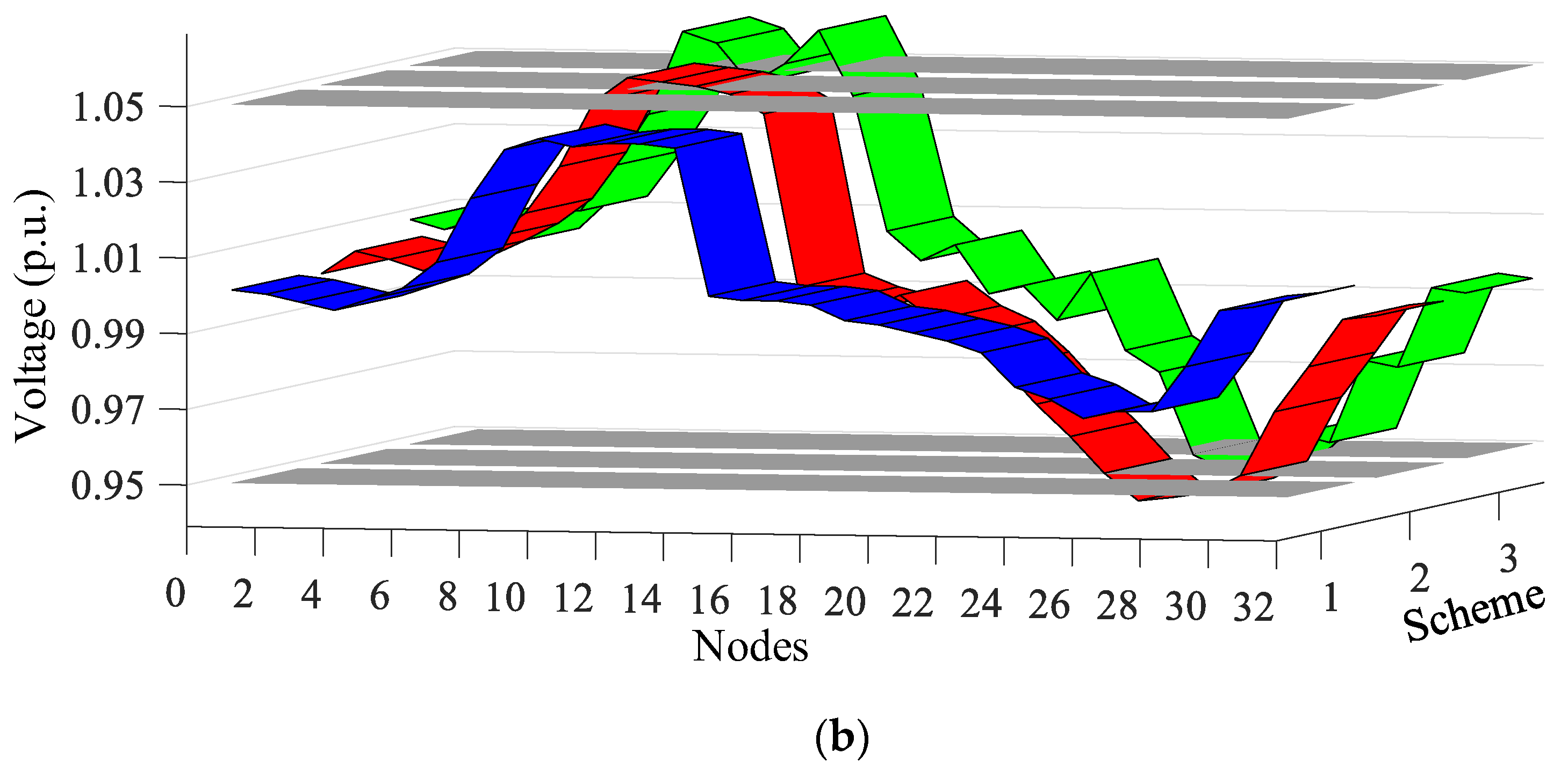
• Scheme 1 performs the proposed optimization scheduling of the distribution network with cluster division for flexible DERs integrated into smart-building systems in Section 3.
• Scheme 2 adopts the centralized optimization scheduling of the distribution network without considering the cluster division.
• Scheme 3 is the initial distribution network before the optimization scheduling.

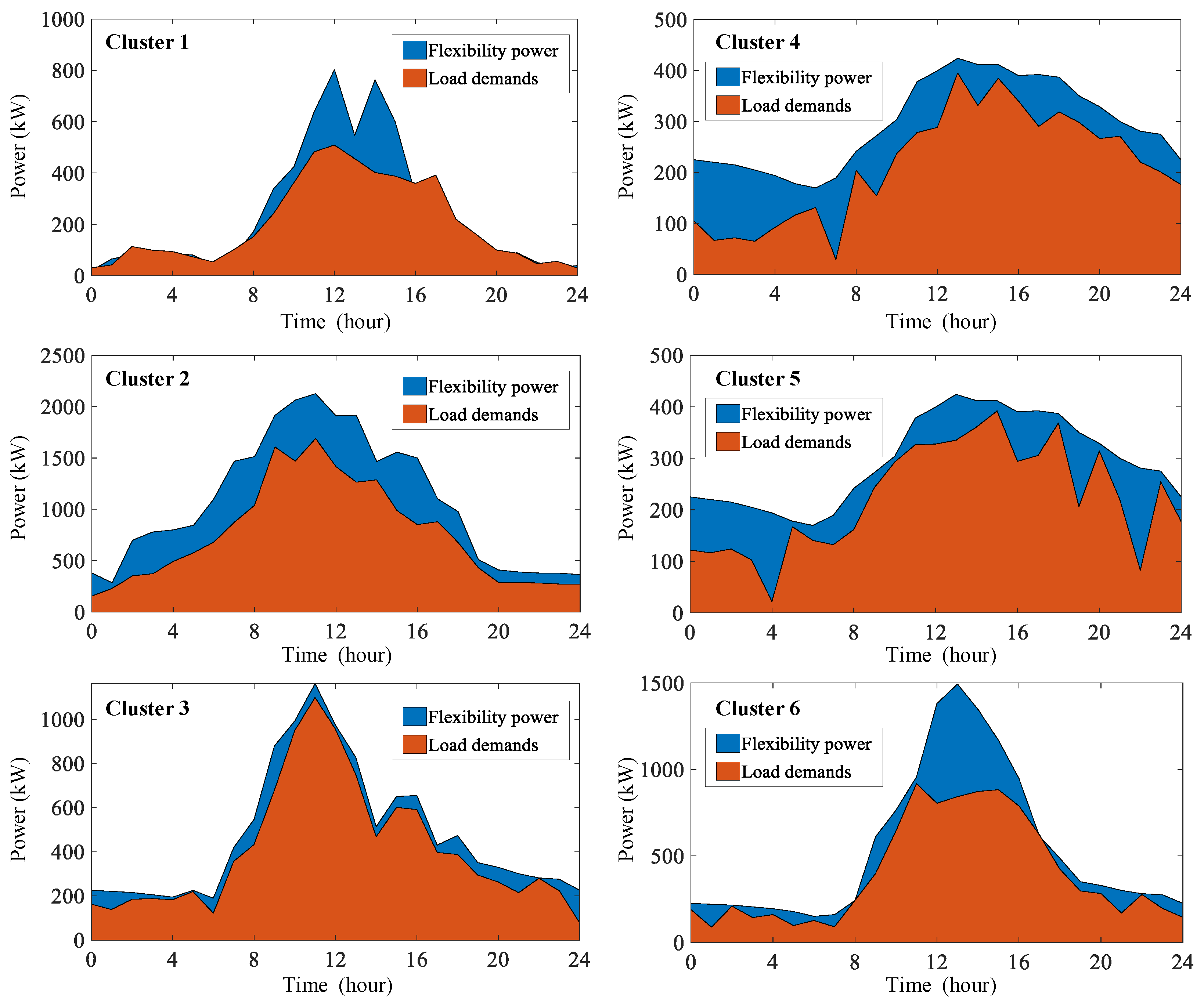
4.3.1. Cluster Division of Building-Integrated Flexible DERs

Considering the differences in node-voltage amplitude, power injection, and load demands at different times, the detailed data of each node at noon is exploited for cluster division. Figure 8 depicts the function curves for the cluster division index of building-integrated DERs corresponding to the number of different clusters. It can be found that the index function achieves the maximum value $\gamma =0.92$ when the number of clusters is divided into 6. Therefore, the result of the optimal cluster division at $K=6$ is shown in Figure 9.

4.3.2. Flexible Regulation Capacity Results of Building-Integrated Flexible DERs

Figure 10 illustrates the flexible regulation capacity of building-integrated flexible DERs based on the flexibility constraint space superimposed by Minkowski Sum. It can be observed from Figure 10 that the self-consistent rate is allowed to reflect the contribution of different flexibility resources to the flexibility balance of the power grid. For instance, the flexibility power region of building-integrated flexible DERs in Cluster 2 is larger than that of Cluster 1. In addition, the sum of the total amount of BIPV generation and the regulation capacity of building-integrated flexible DERs can satisfy the total load demands within Cluster 2, indicating that Cluster 2 achieves complete self-consistency of active power. On the contrary, the total load demands within Cluster 1 are greater than the sum of the total amount of BIPV generation and the regulation capacity of building-integrated flexible DERs at time $t=4$ and $t=20$, thus giving rise to flexibility power deficiency.

4.3.3. Optimization Scheduling Results with Schemes 1–3

The power-loss and the node-voltage amplitude with Schemes 1–3 are illustrated in Figure 11, where the node-voltage at noon is selected for analysis since the generation of BIPVs reaches the peak at that time.

It can be found that the optimized system power loss with Scheme 1 is lower than that with Scheme 2 due to the comprehensive scheduling of the BIPV generation and the regulation capacity of building-integrated flexible DERs within clusters. In addition, the voltage-regulation effect of the centralized active power–reactive power cooperative optimization of the distribution network is unsatisfactory, maintaining the node voltage over the limit. However, since building-integrated flexible DERs are involved in the cluster power regulation, the node-voltage amplitude with Scheme 1 is within the specified range.

Table 2. Comparative economic performance results.

Scheme	Operation Cost (USD)	Network Loss Cost (USD)	Flexibility Deficiency Cost (USD)
1	5697.8	3089.6	2608.2
2	6027.1	3254.3	2872.8
3	6452.6	3438.1	3014.5

summarizes the statistical data of comparative economic performance results with Schemes 1 and 2, including the total cost, the operational cost, the power-loss cost, and the flexibility deficiency cost. Compared to Scheme 2, Scheme 1, considering the flexibility of building-integrated flexible DERs, can better estimate the flexibility regulation capacity, and thus, the operational cost and flexibility deficiency cost can be reduced by 11.69% and 9.21%, respectively. Consequently, Scheme 1 outperforms Schemes 2 and 3 on the economic merits and voltage regulation.

5. Conclusions

In this paper, an optimal active–reactive power collaborative scheduling model for building flexible DER clusters is proposed to resolve the uncertainties from the renewable energy in the distribution network. The key findings of this study are as follows: (1) The developed cluster division algorithm considering structural and functional indexes can achieve independent autonomy within clusters and coordinated interaction among clusters, contributing to decreasing the whole network loss; (2) Since the customized virtual battery models integrate and quantify the regulation capacity of flexible resources, the flexibility deficiency cost can be reduced by 9.21%; (3) The developed optimal active–reactive power collaborative scheduling model can achieve a better performance in economic merits and voltage regulation than the centralized optimization scheduling of a distribution network without considering the cluster division, whose operational cost can be decreased by 11.69%. In this article, the building-integrated flexible DERs, including BIES, BIEV, and BITC, were acknowledged as the resources on the demand side. Further research will focus on the collaborative flexibility regulation capacity of building-integrated flexible DERs on the supply side and demand side.

References

1. IEA. World Energy Outlook 2022:C. Available online: https://iea.blob.core.windows.net/assets/75cd37b8-e50a-4680-bfd7-0424e04a1968/WorldEnergyOutlook2022.pdf (accessed on 10 November 2022).
2. Xue, Q.W.; Wang, Z.J.; Chen, Q.Y. Multi-objective optimization of building design for life cycle cost and CO2 emissions: A case study of a low-energy residential building in a severe cold climate. Build. Simul. 2022, 15, 83–98. [Google Scholar] [CrossRef]
3. Bhattarai, B.P.; Cerio Mendaza, I.D.; Myers, K.S.; Bak-Jensen, B.; Paudyal, S. Optimum Aggregation and control of spatially distributed flexible resources in smart grid. IEEE Trans. Smart Grid 2018, 9, 5311–5322. [Google Scholar] [CrossRef]
4. Tsaousoglou, G.; Sartzetakis, I.; Makris, P.; Efthymiopoulos, N.; Varvarigos, E.; Paterakis, N.G. Flexibility aggregation of temporally coupled resources in real-time balancing markets using machine learning. IEEE Trans. Ind. Informat. 2022, 18, 4342–4351. [Google Scholar] [CrossRef]
5. Kermani, M.; Adelmanesh, B.; Shirdare, E. Intelligent energy management based on SCADA system in a real microgrid for smart building applications. Renew. Energy 2021, 171, 1115–1127. [Google Scholar] [CrossRef]
6. Eini, R.; Linkous, L.; Zohrabi, N.; Abdelwahed, S. Smart building management system: Performance specifications and design requirements. J. Build. Eng. 2021, 39, 102222. [Google Scholar] [CrossRef]
7. Li, C.; Dong, Z.; Li, J.; Li, H. Optimal control strategy of distributed energy storage cluster for prompting renewable energy accomodation in distribution network. Automat. Electron. Power Syst. 2018, 45, 76–83. [Google Scholar]
8. Hu, W.Q.; Wu, Z.X.; Lv, X.X.; Dinavahi, V. Robust secondary frequency control for virtual synchronous machine-based microgrid cluster using equivalent modeling. IEEE Trans. Smart Grid. 2021, 12, 2879–2889. [Google Scholar] [CrossRef]
9. Yu, S.; Liu, N.; Zhao, B. Multi-agent Classified Voltage Regulation Method for Photovoltaic User Group. Automat. Electron. Power Syst. 2022, 46, 20–41. [Google Scholar]
10. Ding, M.; Liu, X.F.; Bi, R.; Hu, D. Method for cluster partition of high-penetration distributed generators based on comprehensive performance index. Automat. Electron. Power Syst. 2018, 42, 47–52. [Google Scholar]
11. Kyriakou, D.G.; Kanellos, F.D. Optimal Operation of Microgrids Comprising Large Building Prosumers and Plug-in Electric Vehicles Integrated into Active Distribution Networks. Energies 2022, 15, 6182. [Google Scholar] [CrossRef]
12. Kyriakou, D.G.; Kanellos, F.D. Energy and power management system for microgrids of large-scale building prosumers. IET Energy Syst. Integr. 2023, 5, 228–244. [Google Scholar] [CrossRef]
13. Farinis, G.Κ.; Kanellos, F.D. Integrated energy management system for microgrids of building prosumers. Electr. Power Syst. Res. 2021, 198, 107357. [Google Scholar] [CrossRef]
14. Bian, X.Y.; Sun, M.Q.; Dong, L.; Yang, X.W. Distributed source-load coordinated dispatching considering flexible aggregated power. Automat. Electron. Power Syst. 2021, 45, 89–98. [Google Scholar]
15. Li, Z.H.; Li, T.; Wu, W.C. Minkowski sum based flexibility aggregating method of load dispatching for heat pumps. Automat. Electron. Power Syst. 2019, 43, 14–21. [Google Scholar]
16. Zhao, W.M.; Huang, H.J.; Zhu, J.Q. Flexible resource cluster response based on inner approximate and constraint space integration. Power Syst. Technol. 2023, 47, 2621–2629. [Google Scholar]
17. Jian, J.; Li, P.; Ji, H.R.; Bai, L.Q. DLMP-based quantification and analysis method of operational flexibility in flexible distribution networks. IEEE Trans. Sustain. Energy 2022, 13, 2353–2369. [Google Scholar] [CrossRef]
18. Shao, C.Z.; Ding, Y.; Wang, J.H.; Song, Y.H. Modeling and integration of flexible demand in heat and electricity integrated energy system. IEEE Trans. Sustain. Energy 2018, 19, 361–370. [Google Scholar] [CrossRef]
19. Majidi, M.; Zare, K. Integration of smart energy hubs in distribution networks under uncertainties and demand response concept. IEEE Trans. Power Syst. 2019, 34, 566–574. [Google Scholar] [CrossRef]
20. Xue, J.R.; Cao, Y.J.; Shi, X.H.; Zhang, Z. Coordination of multiple flexible resources considering virtual power plants and emergency frequency control. Appl. Sci. 2023, 13, 6390. [Google Scholar] [CrossRef]
21. Li, W.; Wei, J.; Cao, Y.; Ma, R.; Zhang, H.; Tian, X. A quantitative assessment method for power system flexibility based on probabilistic optimal power flow. Mod. Electr. Power 2023, 40, 1–12. [Google Scholar]
22. Lin, Z.; Li, H.; Su, Y. Evaluation and expansion planning method of a power system considering flexible carrying capacity. Power Syst. Prot. Control 2021, 49, 46–57. [Google Scholar]
23. Sun, H.; Fan, X.; Hu, S. Internal and external coordinated bidding strategy of virtual power plants participating in the day ahead power market. Power Syst. Technol. 2022, 46, 1248–1262. [Google Scholar]
24. Cao, Y.; Zhou, B.; Chung, C.Y.; Shuai, Z.; Hua, Z.; Sun, Y. Dynamic modelling and mutual coordination of electricity and watershed networks for spatio-temporal operational flexibility enhancement under rainy climates. IEEE Trans Smart Grid 2023, 14, 3450–3464. [Google Scholar] [CrossRef]
25. Zhang, C.; Liu, Q.; Zhou, B.; Chung, C.Y.; Li, J.; Zhu, L.; Shuai, Z. A central limit theorem-based method for DC and AC power flow analysis under interval uncertainty of renewable power generation. IEEE Trans. Sustain. Energy 2023, 14, 563–575. [Google Scholar] [CrossRef]
26. Wang, X.; Zhang, H.; Zhang, S. Game model of virtual power plant composed of wind power and electric vehicles participating in power market. Autom. Electr. Power Syst. 2019, 43, 155–162. [Google Scholar]
27. Zhang, W.; Song, J.; Guo, M. Load balancing management strategy of virtual power plant considering electric vehicle charging demand. Autom. Electr. Power Syst. 2022, 46, 118–126. [Google Scholar]
28. Zhu, Y.W.; Zhang, T.; Ma, Q.S.; Fukuda, H. Thermal performance and optimizing of composite trombe wall with temperature-controlled dc fan in winter. Sustainability 2022, 14, 3080. [Google Scholar] [CrossRef]
29. Sun, Z.Q.; Si, W.G.; Luo, S.J.; Zhao, J. Real-time demand response strategy of temperature-controlled load for high elastic distribution network. IEEE Access 2021, 9, 69418–69425. [Google Scholar] [CrossRef]
30. Huang, H.; Nie, S.L.; Jin, L.; Wang, Y.Y.; Dong, J. Optimization of peer-to-peer power trading in a microgrid with distributed pv and battery energy storage systems. Sustainability 2020, 12, 923. [Google Scholar] [CrossRef]
31. Deng, Y.S.; Jiao, F.S.; Zhang, J.; Li, Z.G. A Short-Term Power Output forecasting model based on correlation analysis and elm-lstm for distributed PV system. J. Electr. Comput. Eng. 2020, 2020, 2051232. [Google Scholar]
32. Li, J.Y.; Khodayar, M.E.; Wang, J.; Zhou, B. Data-driven distributionally robust co-optimization of P2P energy trading and network operation for interconnected microgrids. IEEE Trans. Smart Grid 2021, 12, 5172–5184. [Google Scholar] [CrossRef]
33. Dhaifallah, M.; Alaas, Z.; Rezvani, A.; Le, B.N.; Samad, S. Optimal day-ahead economic/emission scheduling of renewable energy resources based microgrid considering demand side management. J. Build. Eng. 2023, 76, 107070. [Google Scholar] [CrossRef]
34. Pandžić, H.; Marales, J.; Conejo, A.; Kuzle, I. Offering model for a virtual power plant based on stochastic programming. Appl. Energy 2013, 105, 282–292. [Google Scholar] [CrossRef]
35. Khani, H.; El-Taweel, N.; Farag, H.E.Z. Supervisory scheduling of storage-based hydrogen fueling stations for transportation sector and distributed operating reserve in electricity markets. IEEE Trans. Ind. Inform. 2020, 16, 1529–1538. [Google Scholar] [CrossRef]
Figure 1. Typical modalities of a smart-building system.
Buildings 13 02854 g001
Figure 2. VB model and the grid-connected operation status of BIEV.
Buildings 13 02854 g002
Figure 3. VB model principle of TCL in a smart-building system.
Buildings 13 02854 g003
Figure 4. Principle of second-order cone relaxation.
Buildings 13 02854 g004
Figure 5. Flowchart of the proposed method.
Buildings 13 02854 g005
Figure 6. Modified IEEE 33-bus distribution system with building-integrated flexible DERs.
Buildings 13 02854 g006
Figure 7. Scenario generation and reduction results of PV outputs at node 24: (a) initial scenarios; (b) reduced scenarios.
Buildings 13 02854 g007
Figure 8. Building-integrated resource cluster division index function curves.
Buildings 13 02854 g008
Figure 9. Optimal cluster division result for the distribution network with building-integrated flexible DERs.
Buildings 13 02854 g009
Figure 10. Flexible regulation capacity of the clusters of the building-integrated flexible DERs.
Buildings 13 02854 g010
Figure 11. Comparative results with Schemes 1–3. (a) The 24 h network loss; (b) The node voltage at noon.
Buildings 13 02854 g011aBuildings 13 02854 g011b