Ground Deformation Monitoring for Subway Structure Safety Based on GNSS

Abstract

Ground deformation poses a serious threat to the safety of subway structures. Consequently, intelligent and efficient automated safety monitoring of ground deformation along the subway has become urgent. Traditional engineering observation methods have the disadvantages of difficulties with datum selection, non-automation, and poor reliability. A ground deformation monitoring system for subway structure safety based on the Global Navigation Satellite System (GNSS) was established and validated through experimental comparisons with traditional precision leveling in this study. Based on the GNSS monitoring points, the continuous kinematic observation GNSS data of ground deformation along the subway line were obtained; a joint robust local mean decomposition (RLMD)–singular value decomposition (SVD) noise-reduction processing method for GNSS signals was proposed to realize the real-time and high-precision monitoring of ground deformation. The results show that the proposed combined noise-reduction method can reduce the maximum noise amplitude by 86%. When compared with the accuracy of the traditional precision leveling method, it was determined that the vertical positioning accuracy of the deformation monitoring system is greater than 2.7 mm, the horizontal positioning accuracy is greater than 1.3 mm, and the measurement error is less than 1.5 mm. The deformation monitoring system has the advantages of convenience, automation, and high accuracy and can be applied to ground deformation monitoring for subway structures.

1. Introduction

With the acceleration of China’s urban development and infrastructure construction, the subway’s structural safety has become a significant concern. Subway construction, building construction along existing subways, tunnel foundation settlement, and underground crossing project construction all affect the structural safety of the original subway tunnels [1]. Therefore, to ensure the safety of existing subway tunnels and those under construction, it is essential to conduct long-term continuous deformation monitoring of certain key areas and major projects along the subway lines. Consequently, continuous ground deformation monitoring along the subway is needed to ensure safety during its operating period [2]. However, several problems exist in monitoring ground deformation along the subway line: (1) it is difficult to find a stable reference point in the subway area; (2) the long-distance measurement error of the reference point is large; (3) traditional deformation monitoring of ground deformation along the subway is mainly based on manual monitoring, with low observation efficiency, insufficient continuity, real-time performance, and the consumption of significant manpower and material resources [3,4]; and (4) it is difficult to find hidden engineering problems and promptly analyze development trends. It is difficult or even impossible to observe ground subsidence under severe weather conditions involving rain, snow, and ice; thus, finding an alternative method for the real-time deformation monitoring of ground subsidence along the subway is required.

The rapid development and highly Integrated application of satellite positioning, computers, wireless communication, and data management technologies provide reliable technical support for solving the problem of real-time, continuous, all-weather settlement monitoring. Among these technologies, satellite positioning based on big data technology has high-precision, automation, all-weather operation, a high data collection frequency, high reliability, and wide application area characteristics [5,6], making it superior to other means of meeting safety supervision requirements. These properties make it ideal for overcoming the previously mentioned engineering observation problems. Using GNSS technology to observe the deformation along the subway line can prevent errors caused by geoid disparity and gravity anomalies, making it more reasonable and feasible than level measurement technology.

Many researchers have conducted extensive research on the application of the GNSS in engineering. Lee et al. [7] analyzed the accuracy of ground deformation using a GNSS fixed monitoring station located at the Shin-Mangin dam. The root-mean-square error (RMSE) of the ground subsidence obtained by comparing data from the GNSS monitoring station with the D-InSAR (Interferometric Synthetic Aperture Radar) technique was accurate to within 0.7 mm. In addition, a correlation analysis of the ground subsidence obtained using the D-InSAR technique was performed and it was determined that the change in the tides is one of the causes of coastal ground subsidence. Bovenga et al. [8] used various satellite-based SAR data (c-band and x-band) and in situ GNSS measurements to monitor the deformation of the Assisi landslide in Italy. Adamcova et al. [9] investigated the landfill settlement calculation method and proposed a permissive landfill model measured by a displacement simulation system based on the GNSS monitoring data set. Their new model uses the Gauss–Newton iterative method and the Runge–Kutta method to estimate the landfill ground displacement and analyze and mathematically describe the landfill body displacement. Iwahana et al. [10] conducted a high-precision GNSS positioning survey to measure the tundra ground displacement in northern Alaska, along with the maximum thaw depth (TD) and ground moisture measurements from 2017 to 2019. Maximum seasonal and interannual subsidence (44 and 56 cm/year, respectively) were recorded at points near the troughs of degraded ice-wedge polygons or thermokarst lakes. Kyriou et al. [11] performed accurate rockfall mapping by processing GNSS measurement data. However, the mapping uses orthophotos of drone data and 3D images of laser scanning motion. Bayik [12] studied a recent landslide displacement caused by geological structures using advanced techniques for InSAR measurements in highly urbanized areas and GNSS observations in the Beylikdüzü and Esenyurt districts of the Istanbul megacity, Turkey. Lu et al. [13] studied the elevation and azimuth angles of GNSS satellites and conducted a cluster analysis combined with signal-to-noise ratios to determine a similar mode of signal propagation. They plotted the GNSS signal cluster analysis results on geographic prediction trajectory maps and generated high-quality mesh maps for accuracy estimation using the GNSS signals. Finally, using the error assignment method, the environmental characteristics and signal quality were used to estimate the error on the track.

Most current research focuses on observation projects, such as urban railway control network designs [14,15], landslide warnings [16,17,18,19], high fill settlements [20,21,22], ground deformation [23,24,25], and crustal movement [26,27,28,29], achieving good technical results. Fewer studies have addressed GNSS ground deformation along subway lines and GNSS technology is affected by errors, such as satellite ephemeris, tropospheric delay, and multipath effect errors. The measurement accuracy of GNSS technology is usually in the range of 10 mm while the foundation displacements of subways during construction and operation are usually on the millimeter scale [30]. As the accuracy of the predictive analysis is seriously affected by the fact that the useful information of the coordinate sequence receives interference from the noise in the GNSS time series [31,32], data collected directly by GNSS cannot meet the real-time monitoring accuracy requirements for ground settlement deformation along subway lines and final settlement amount predictions.

It is evident that ground deformation poses a serious threat to the safety of subway structures. Realizing the automated safety monitoring of ground deformation intelligently and efficiently along the subway in the process of subway construction and operation needs to be addressed urgently. However, traditional engineering observation methods are associated with problems, such as difficulties with datum selection, low automation, and poor reliability. In this study, the author constructed a ground deformation monitoring system along the subway based on the GNSS and verified the validity of the method through experimental comparison with the traditional precision leveling method. Meanwhile, the deformation monitoring system has the advantages of the convenient selection of the reference point, high automation, and reliability and it can be applied to ground deformation monitoring for subway structure safety.

In this study, based on the GNSS monitoring data, the RLMD–SVD joint method was used to reduce the signal noise and the ground deformation monitoring system for subway structure safety was developed. First, the GNSS control network deployment and measurement was introduced and the continuous kinematic observation GNSS data were obtained. Furthermore, the signal noise was reduced by the SVD-RLMD joint method and the ground deformation monitoring system was constructed. The accuracy of the deformation monitoring system along the subway line was investigated by conducting an experiment using the traditional precision level. The results show that the system can ensure the integrity and accuracy of the observation data and the obtained observation values are essentially consistent with the traditional level observation values.

In this paper, we have proposed a ground deformation monitoring system for subway structure safety based on the GNSS. The RLMD–SVD joint denoising method is introduced in Section 2. Details of the experiment that was conducted are presented in Section 3 and the performance of this method is shown in Section 4. Finally, the conclusion is given in Section 5.

2. Methodology

2.1. High-Precision Calculation of GNSS Data

The high-precision GNSS data processing in the GNSS solution software, which is independently developed by Wuhan University, is key to ensuring the system’s monitoring accuracy. The Software-As-A-Service (SAAS) model corrects the tropospheric hydrostatic delay and the Global Mapping Function (GMF) estimates the tropospheric wet delay using a linear segmentation method without the atmospheric gradient parameters. As the generation of cycle slip interrupts the tracking arc segment continuity of high-precision carrier observations and one week of cycle slip produces approximately a 20 cm deviation on the carrier, accurate, reliable, and real-time cycle slip detection becomes one of the key elements in high-precision real-time deformation monitoring. The total electron content rate (TECR)–Melbourne–Wubbena (MW) joint method [33] was used for real-time periastron detection. The combined MW observations can eliminate the station-star geostationary distance first-order term effects and ionospheric delays, which account for more than 80% of the total ionospheric delays [34], providing a good cycle slip detection quantity during high ionospheric activity periods. By constructing the MW combination method and ignoring the multipath error, a wide path uncertainty $N_{\delta }$ is obtained:

$$N_{\delta }=N_1-N_2=\left({\phi }_1-{\phi }_2\right)-\frac{f_1-f_2}{f_1+f_2}·\frac{f_1{P}_1+f_2{P}_2}{c}+{\epsilon }_{N\delta }$$

(1)

where f₁ and f₂ denote the frequencies;${\phi }_1$,${\phi }_2$,$P_1$,$P_2$, $N_1, \mathrm{and} N_{2 }$denote the wavelengths of the two frequency points, the carrier observation, the pseudo-distance observation, and the ambiguity parameter, respectively; and ${\sum }_{N_b}$ denote the measurement noises corresponding to the observations. The MW method is mainly affected by the pseudo-distance measurement noise due to the high accuracy of the carrier observation.

The ionospheric rate TECR_Φ (k) in TECU/s is:

$$TEC{R}_{\varnothing }\left(k\right)=\frac{TE{C}_{\varnothing }\left(k\right)-TE{C}_{\varnothing }(\left(k-1\right)}{\Delta t}$$

(2)

where $TE{C}_{\varnothing }\left(k\right)$is the total electron content (TEC) of the ionosphere in epoch k:

$$TE{C}_{\varnothing }\left(k\right)=\frac{f_1^2\left[\left(\Delta {\mathrm{L}}_I-\left({\lambda }_1{N}_1-{\lambda }_2{N}_2\right)\right)\right] }{40.3\times {10}^{16}\left(\mathsf{\gamma }-1\right)}$$

(3)

and where γ is the scale factor of the two frequency points, i.e., $f_1$ and $f_2$ are the $L_1$ and $L_2$ frequencies$; L_1$ and $L_2$ denote the carrier waves corresponding to the observations in m; $\Delta L_I$ is the ionospheric residual; and ${\lambda }_1$ and ${\lambda }_2$ denote the wavelengths of the two frequency points.

After ensuring that the carrier-phase data used in the initial calculation is non-cycle slip data, the carrier-phase double-difference observation equation [35] must be established and used to achieve high-precision localization. Assuming the reference station and the monitoring station’s synchronous observation of the k and j satellites, the double-difference carrier phase and double-difference pseudo-range of the observation equations are:

$${\lambda }_i·\Delta \nabla {\mathsf{\Phi }}_i^S=\Delta H^S·\delta X+\Delta \nabla {\rho }^S-{\lambda }_i·\Delta \nabla N_i^S-\Delta \nabla I_i^S+\Delta \nabla T^S+\Delta \nabla {\epsilon }_i^S$$

(4)

$$\Delta \nabla P_i^S=\Delta H^S·\delta X+\Delta \nabla {\rho }^S+\Delta \nabla I_i^S+\Delta \nabla T^S+\Delta \nabla {\epsilon }_{ic}^S$$

(5)

where$\Delta \nabla$ is the double-difference operator, indicating that it combines the double differences between the carrier-phase observations of the two BeiDou satellites and the two stations$, \Delta H^S$ is the coefficient of the position parameter for the single difference between the stars$, \varphi$ is the carrier-phase observation, P is the pseudo-range observation, H is the coefficient of the position parameter$, \rho$ is the geometric distance between the stations, and $\lambda$ is the wavelength of the carrier phase. In addition, N is the ambiguity, I is the ionospheric delay error, the subscript i denotes the frequency, T is the tropospheric delay and satellite orbit error, the superscript denotes the satellite, t is the receiver clock error, and $\epsilon$ is the observation noise.

The reference station coordinates are known and there is no need to calculate the position parameter. Then, the double-difference observation equations are:

$${\lambda }_i·\Delta \nabla {\mathsf{\Phi }}_i^S=\Delta \nabla {\rho }^S-{\lambda }_i·\Delta \nabla N_i^S-\Delta \nabla I_i^S+\Delta \nabla T^S+\Delta \nabla {\epsilon }_i^S$$

(6)

$$\Delta \nabla P_i^S=\Delta \Delta \nabla {\rho }^S+\Delta \nabla I_i^S+\Delta \nabla T^S+\Delta \nabla {\epsilon }_{ic}^S$$

(7)

The unknowns are mainly the carrier-phase ambiguity parameters and the double-difference residuals of various observation errors.

The double-difference observation equations remove receiver clock differences and further attenuate the effects of ionospheric and tropospheric delay errors, whose observation noise and multipath effects are further amplified. For short baselines, the spatial atmospheric conditions of the reference and monitoring stations are highly correlated; after the double difference, the ionospheric and tropospheric delay errors are negligible, with the error sources being mainly multipath errors and observational noise. For medium-range and long-range baselines (30–100 km), the residual tropospheric delay and ionospheric delay errors after the double difference, and even the BeiDou Navigation Satellite System (BDS) broadcast ephemeris orbit errors, are non-negligible.

The stochastic model can reflect the correlation between observations and the random noise level, which affects the accuracy and reliability of the localization results, the success rate of the ambiguity search, and other aspects. Different a priori variances of the original observations result in different weight arrays, affecting the accuracy of the baseline solution results.

The lower the satellite’s elevation angle, the longer the satellite signal path through the atmosphere, which is affected by atmospheric and multipath delays, and the higher the observation noise. The stochastic model usually assumes that the deformation monitoring system carrier-phase observations from the same system all have the same precision σ (σ = σ_BDS). Then, assuming that the individual epoch observations are uncorrelated, the precision of the single-difference observations is such that the variance–covariance array of the entire ith epoch double-difference observations [36] is:

$$D=\left[\begin{array}{c}{D}_1 \\ D_2\\ \cdots \\ D_S\end{array}\right]={\sigma }^2\left[\begin{array}{c}P{\left(1\right)}^{-1} \\ P{\left(2\right)}^{-1} \\ \cdots \\ P{\left(s\right)}^{-1}\end{array}\right]={\sigma }^2{P}^{-1}$$

(8)

where P(i) is the corresponding power array and the least squares estimates of the parameters and their variance–covariance matrices obtained from Equation (7) of the observation equation and Equation (8) of the stochastic model are expressed:

$$X=-{\left(A^{T}PA\right)}^{-1}{A}^{T}PL$$

(9)

$$D_x={\sigma }^2{\left(A^{T}PA\right)}^{-1}$$

(10)

where $\sigma =\frac{V^{T}PV}{n-t}$, n is the total number of double-difference observations, t is the number of unknown parameters, V is the residual vector of the observations, and X is the vector of unknown parameters, including the baseline component and the whole-week ambiguity. $A\left(i\right)={\left[A_1,A_2,\cdots ,A_{m-1}\right]}^T$ is its coefficient matrix and $L\left(i\right)={\left[L_1,L_2,\cdots ,L_{m-1}\right]}^T$ is the difference between the observed and computed values derived from the approximation of the unknown parameters, which can be obtained by substituting Equation (9) into Equation (7).

Based on the variance calculated in the above equation, the variance array of double-difference observations can be calculated by combining the single-difference operator and the double-difference operator using the law of error propagation.

The Kalman filter estimation method, which is then extended by the parameter estimation method, is given by:

$$X_{k+1}={\Phi }_{k+1,k}{\widehat{X}}_k+w_k$$

(11)

$$L_{k+1}=H_{k+1}{X}_k+\left({\tilde{L}}_k-H_{k+1}{\tilde{X}}_k\right)+v_k$$

(12)

The above equations, Equations (11) and (12), are the state and observation equations after linearization, respectively, where $x_{k+1}$ is the state vector at the moment of k + 1 epochs and ${\widehat{x}}_k$ is the state vector at the moment of k epochs after updating the estimation with Kalman filtering. Additionally, ${\varphi }_{k+1}$ and ${\omega }_k$ are the corresponding state transfer and kinematic noise matrices, respectively, $L_{k+1}$ and $H_{k+1}$ are the observation vector and coefficient matrices, respectively, $\left({\tilde{L}}_k-{\tilde{H}}_{k+1}{\tilde{X}}_k\right)$can be regarded as the control input, and ${\upsilon }_k$ is the observation noise vector. Finally, combined with the reference station’s known coordinates, the monitoring station’s high-precision coordinates complete the static relative positioning solution process. The more epochs are involved in the calculation, the higher the positioning accuracy.

2.2. Robust Local Mean Decomposition (RLMD)

The GNSS monitoring signal consists of three main parts: the actual vibration of the structure, the multipath error, and random noise. Among them, the multipath error is mainly concentrated in the frequency band from 0 to 0.2 Hz [37], which is often suppressed by robust local mean decomposition.

Local mean decomposition (LMD) is an adaptive time–frequency representation proposed by Smith et al. [38] in 2005, which essentially adaptively decomposes any signal x(t) into several product functions (PFs) and the sum of the remaining components in decreasing frequency order based on the envelope characteristics of the signal, namely:

$$x\left(t\right)={{\displaystyle \sum }}_{p=1}^{k}P{F}_p\left(t\right)+u_k{\displaystyle \mathit{\left(}t\mathit{\right)}}$$

(13)

where each PF is obtained by multiplying the envelope function by the pure frequency modulation function.

However, this method may suffer from endpoint effects and modal aliasing to some extent. To solve this problem, Liu et al. [39] proposed a robust local mean decomposition method that improved the LMD by optimizing the boundary conditions, envelope estimation, and iterative stopping criterion. The specific optimization process is:

(1) Boundary conditions: the symmetric points at the left and right ends of the signal are determined by the mirror extension algorithm;

(2) Envelope estimation:

Firstly, it is necessary to calculate the mean and standard deviation, which correspond to the step between the smooth local mean and smooth local amplitude, respectively:

$$b\left(k\right)=\left(edge\left(k\right)+edge\left(k+1\right)\right)/2)$$

(14)

$$u_s={{\displaystyle \sum }}_{k=1}^{N_b}b\left(k\right)B\left(k\right)$$

(15)

$${\gamma }_s=\sqrt{{{\displaystyle \sum }}_{k=1}^{N_b}(b{\left(k-u_s\right)}^{2}B\left(k\right)}$$

(16)

where $N_b$ is the number of steps; $B\left(k\right)$ denotes the probability of counting the set of steps using the histogram bin counts when the probability of each bin is obtained; and $edge\left(k\right)$ denotes the edge of the bin; $N_b$ denotes the number of bins.

Then, a reasonable fixed subset size ${\lambda }^{*}$ is obtained according to statistical theory, namely:

$${\lambda }^{*}=odd\left(u_s+3\times {\gamma }_s\right)$$

(17)

(3) Iterative stopping criterion: minimize the following functions:

$$f\left(x\right)=RMSE\left(z\left(t\right)\right)+EK\left(z\left(t\right)\right)$$

(18)

where $RMSE\left(z\left(t\right)\right)$ and $EK\left(z\left(t\right)\right)$ can be expressed as:

$$RMSE\left(z\left(t\right)\right)=\sqrt{\frac{1}{N}{{\displaystyle \sum }}_{i=1}^n{\left(z\left(t\right)\right)}^2}$$

(19)

$$EK\left(z\left(t\right)\right)=\frac{\frac{1}{N}{{\displaystyle \sum }}_{i=1}^n{\left(z\left(t\right)-\overline{z}\right)}^4}{{\left(\frac{1}{N}{{\displaystyle \sum }}_{i=1}^n{\left(z\left(t\right)-\overline{z}\right)}^2\right)}^2}-3$$

(20)

where $z\left(t\right)$ is the zero-baseline envelope signal; $\overline{z}$ is the average value of the zero-baseline envelope signal; and $\overline{z}$ is the expression for:

$$\overline{z}=\frac{1}{N}{{\displaystyle \sum }}_{i=1}^{n}z\left(t\right)$$

(21)

2.3. Singular Value Decomposition for Noise Reduction

As the GNSS monitoring source signal x(i) (i = 1, 2, 3, …, N) of the ground deformation along the subway line after preliminary noise reduction is one-dimensional, it is necessary to construct the Hankel matrix D for singular value decomposition based on the phase space reconstruction theory [40]:

$$\mathrm{D}=\left[\begin{array}{cccc}\mathrm{x}\left(1\right)& \mathrm{x}\left(2\right)& \hfill \dots & \mathrm{x}\left(\mathrm{n}\right)\\ \mathrm{x}\left(2\right)& \mathrm{x}\left(3\right)& \hfill \dots & \mathrm{x}\left(\mathrm{n}+1\right)\\ ⋮& ⋮& ⋮\hfill & ⋮\\ \mathrm{x}\left(\mathrm{m}\right)& \mathrm{x}\left(\mathrm{m}+1\right)& \dots \hfill & \mathrm{x}\left(\mathrm{N}\right)\end{array}\right]$$

(22)

To achieve good noise reduction, the values of m and n when constructing the matrix should meet the following requirements: when N is even, m = N/2 + 1, n = N/2 and when N is odd, m = (N − 1)/2, n = (N + 1)/2 + 1.

Assuming that r is the rank of D, the singular value decomposition of D is:

$$D=U\left[\begin{array}{cc}\Sigma & 0\\ 0& 0\end{array}\right]V^T$$

(23)

where U is an m × m order orthogonal matrix, Σ is an r × r order diagonal matrix, V is an n × n order orthogonal matrix, and 0 is a zero matrix. The elements in the diagonal matrix are the non-zero singular values λi in decreasing order, i.e., λ₁ ≥ λ₂ ≥ … ≥ λ_r.

A series of non-zero singular values are obtained through decomposition, including useful signals and noise. The larger singular values reflect the true signal. From the (i + 1)th order, the singular values become significantly smaller and subsequent singular values can be regarded as corresponding to the singular values of the noise signal. Only the singular values of the first i true signals in the Σ matrix are retained; the remaining singular values are set to zero, with the construction of a new diagonal matrix in the form of the Hankel matrix. The number of singular values is chosen to be twice the number of primary source signal frequencies and does not vary with the number of rows in the reconstruction matrix.

$${\Sigma }^{\prime }=diag\left({\lambda }_1,{\lambda }_2,\dots ,{\lambda }_i,0,0\dots ,0\right)$$

(24)

The signal after noise reduction is obtained by averaging the elements on the inverse diagonal of the newly constructed diagonal matrix.

2.4. Ground Deformation Monitoring System along the Subway Based on the GNSS Monitoring Signal

Ground deformation along the subway line is inevitable and it is difficult to achieve fast and accurate real-time monitoring of these displacements, deformations, and settlements using conventional manual measurement methods. This is due to its heavy workload, accumulated errors, and long observation period. To address the above shortcomings, establishing a ground deformation monitoring system based on the GNSS can achieve continuous observation of the subway during its operation period.

A ground deformation study area was set up near Metro Line 6 in Hanyang District, Wuhan, Hubei Province, with the measurement point layout shown in Figure 1; the specific arrangement is shown in Section 3.1.1.

First, the relative positioning between one reference station and five monitoring points is measured using BeiDou satellites. The position information of each monitoring point in different periods is obtained through relative positioning and the displacement information of each monitoring point in different periods is obtained by comparing it to the results of the first period. Then, the GNSS signals are resolved with high density and the RLMD–SVD joint denoising method eliminates various environmental influence error factors to obtain the displacement information with millimeter-level accuracy. This information is sent to the system monitoring cloud platform through the data transmission system and the cloud platform forms the time-range deformation parameters and related technical indexes of each structure. At the same time, early warnings can be carried out for deformation values exceeding the set threshold.

According to the actual urban subway, the GNSS automated monitoring network system for ground deformation along the subway consists of four parts: sensor subsystem, data transmission subsystem, auxiliary support system, and data processing and control subsystem, as shown below:

(1)

Sensor subsystem: consists of each GNSS monitoring unit and is responsible for collecting monitoring data from ground deformation monitoring points along the subway;

(2)

Data transmission subsystem: responsible for the real-time transmission of the data collected by the sensor system to the control center. Specific transmission methods generally use optical fiber, wireless bridges, and other media for reliable, effective, and stable performance. It uses multiple methods to coexist, even solving problems related to long distances and wiring trouble, and can also be used to set up a wireless base station;

(3)

Auxiliary support system: consists of a monitoring field and monitoring center to assist the normal operation of all GNSS automated monitoring system equipment, including power distribution and UPS, lightning protection, integrated wiring, field cabinets, and other subsystems;

(4)

Data processing and control subsystem: consists of a small computer system, server system, and software system located in the monitoring center.

Based on the RLMD–SVD joint denoising method, the flow chart of the constructed ground deformation monitoring platform along the subway is shown in Figure 2.

3. Results

3.1. GNSS Measurement Points

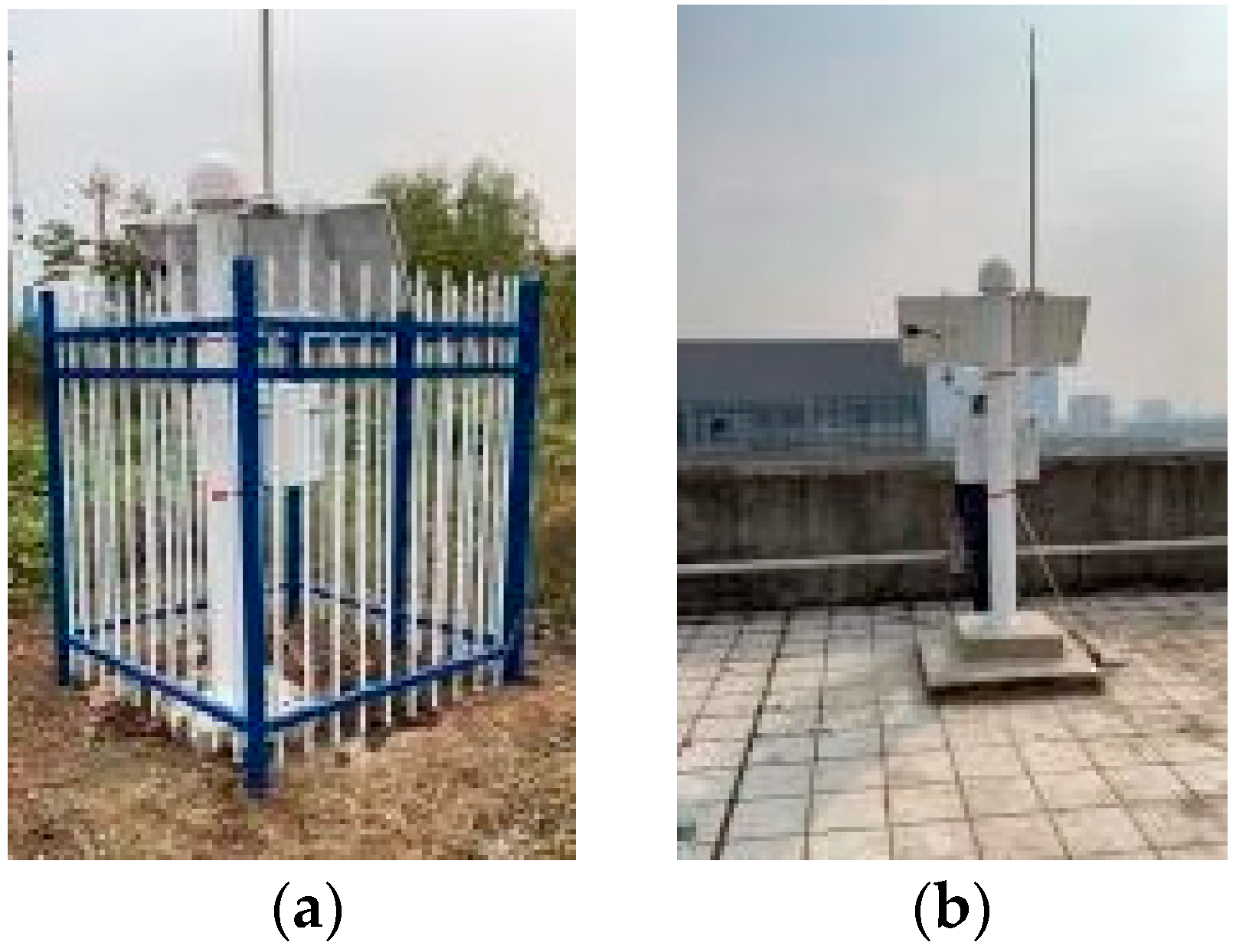
3.1.1. Integrated BeiDou Monitoring Equipment

There are typical periodic deformations in the key settlement area along the subway, and the BDS technology is used to monitor the deformation to obtain the high temporal and spatial characteristics of the deformations. DT100 is a Beidou GNSS receiver independently developed by Wuhan University, which was adopted during instrument selection to ensure the accuracy of the measurement results.

The BDS monitoring equipment is shown in Figure 3a, including the DT100 full-frequency point measurement receiver, antennas, digital transmission radios, wireless data transmission units (DTUs), solar panels, batteries and their controllers, and encapsulated enclosures. The DT100 has a sampling frequency of 1 hz; the horizontal accuracy is ($2.5 \mathrm{mm}+d\times 0.5 \mathrm{mm}/\mathrm{km}$) and the vertical accuracy is ($5 \mathrm{mm}+d\times 0.5 \mathrm{mm}/\mathrm{km}$), where d is the distance in km from the measurement point. For real-time kinematic measurement, the accuracies were ($8 \mathrm{mm}+d\times 1 \mathrm{mm}/\mathrm{km}$) horizontally and ($15 \mathrm{mm}+d\times 1 \mathrm{mm}/\mathrm{km}$) vertically, meeting the observation requirements. The BDS measurement station was installed on the surface of a fill structure along the subway line, which has a greater thickness of fill soil and a spacious top, as shown in Figure 3b.

3.1.2. Layout of Measurement Points

According to the relevant research results [41], the relative positioning accuracy of the deformation monitoring system is related to the baseline length and the difference in vertical displacement accuracy is small when the baseline length is within 5 km. Therefore, to ensure the accuracy of BDS relative positioning technology, the baseline length of the ground deformation monitoring along the subway was controlled to within 5 km. Alternate measurement points were selected from the ground deformation monitoring station locations along the subway; the installation location of the measurement point is shown as depicted in Figure 3b. Then, the actual observation data collection was carried out at these points and data quality analysis was conducted using the TEQC [42,43] GNSS data quality analysis software.

Finally, the alternate points were screened by integrating the shape of the point distribution, the signal quality, and other factors and five sets of DT100 full-frequency receivers were set up above the ground along the subway with a large settlement. Five BDS deformation observation stations (BDT1–BDT5) were set up and the arrangement of the stations is shown in Figure 1. Observation stations BDT2–BDT5 were located in the soft soil layer above the ground along the subway. The terrain in this area is relatively flat and the ground is primarily a farmland base, surrounded by roads, houses, and factories; it was used to observe the ground deformation along the subway. Observation station BDT1 was located off the road and was used to observe the ground deformation outside the soft soil layer. A GNSS-CORS (Continuously Operating Reference Station) receiver was used for continuous operation as the reference station for data and was installed on the roof of a nearby subway repair shop with a stable structure and open top as the final monitoring deployment plan. Both stations used wireless transmission and solar power to establish an independent ground deformation monitoring station along the subway. The measurement station is shown in Figure 4a and the CORS reference station is shown in Figure 4b.

The monitoring and reference stations used BDS receivers to receive the monitoring signals. The difference data were sent to the monitoring station through the digital transmission radio to perform real-time difference calculations to obtain the RTK positioning results of the monitoring station. The original observation data, such as the carrier phase of the satellite signals, were sent to the remote monitoring center via the DTUs. Each monitoring point continuously tracked and observed the satellite signals for a long time and transmitted the GNSS observation data to the control center in real time via the data communication network. The observation data of each reference station were combined with the start coordinates of the control center through the software quasi-real-time solution process, finally obtaining the three-dimensional coordinates of each monitoring point.

The GNSS remote ground deformation monitoring center along the subway was a network server with a fixed IP address that collected data from the reference and monitoring stations. The RTK positioning results received from the monitoring station were displayed kinematically. A large amount of carrier-phase data from the integrated reference station and the monitoring station was resolved over a long period for static relative positioning to obtain more accurate positioning results as the primary basis for the rail transit deformation monitoring.

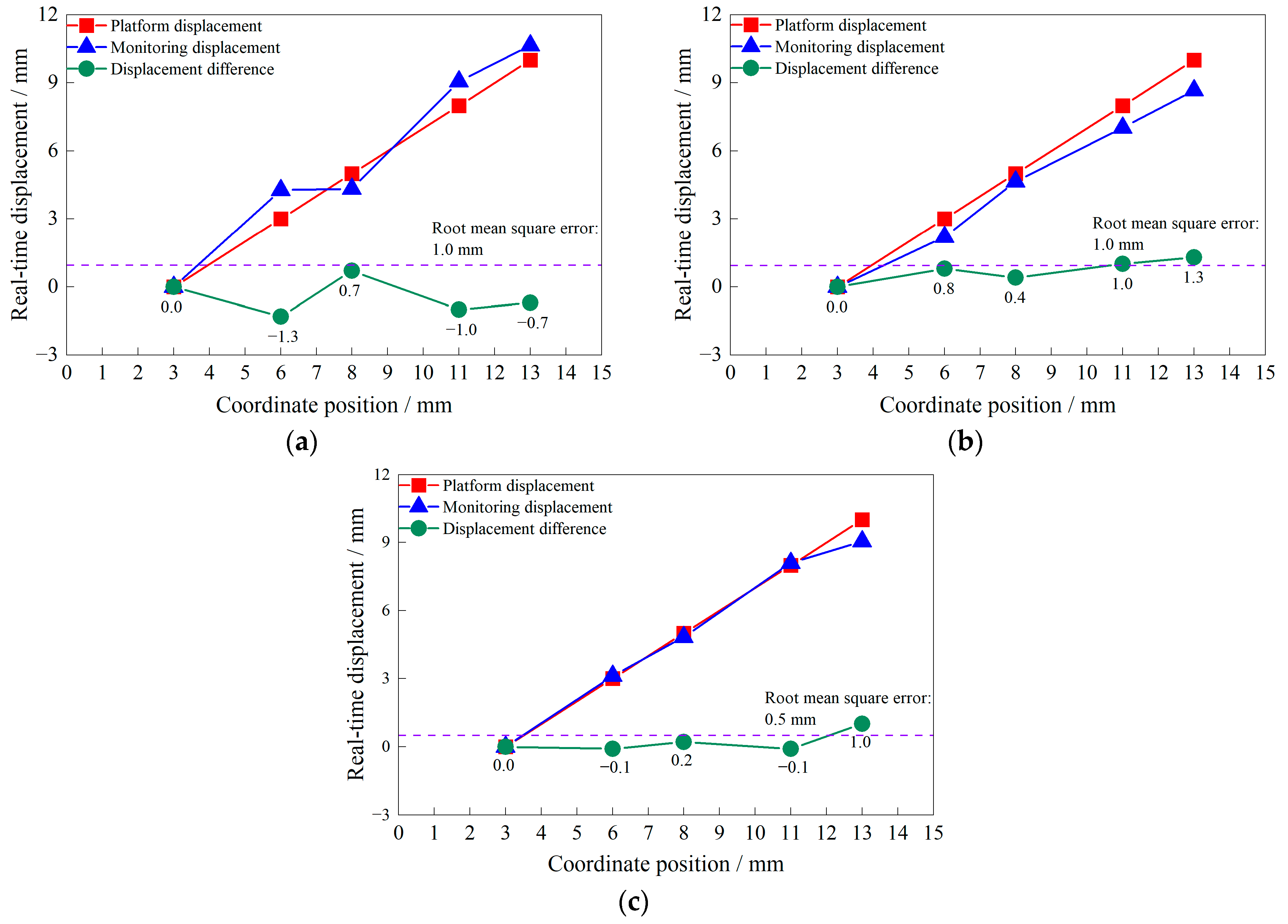
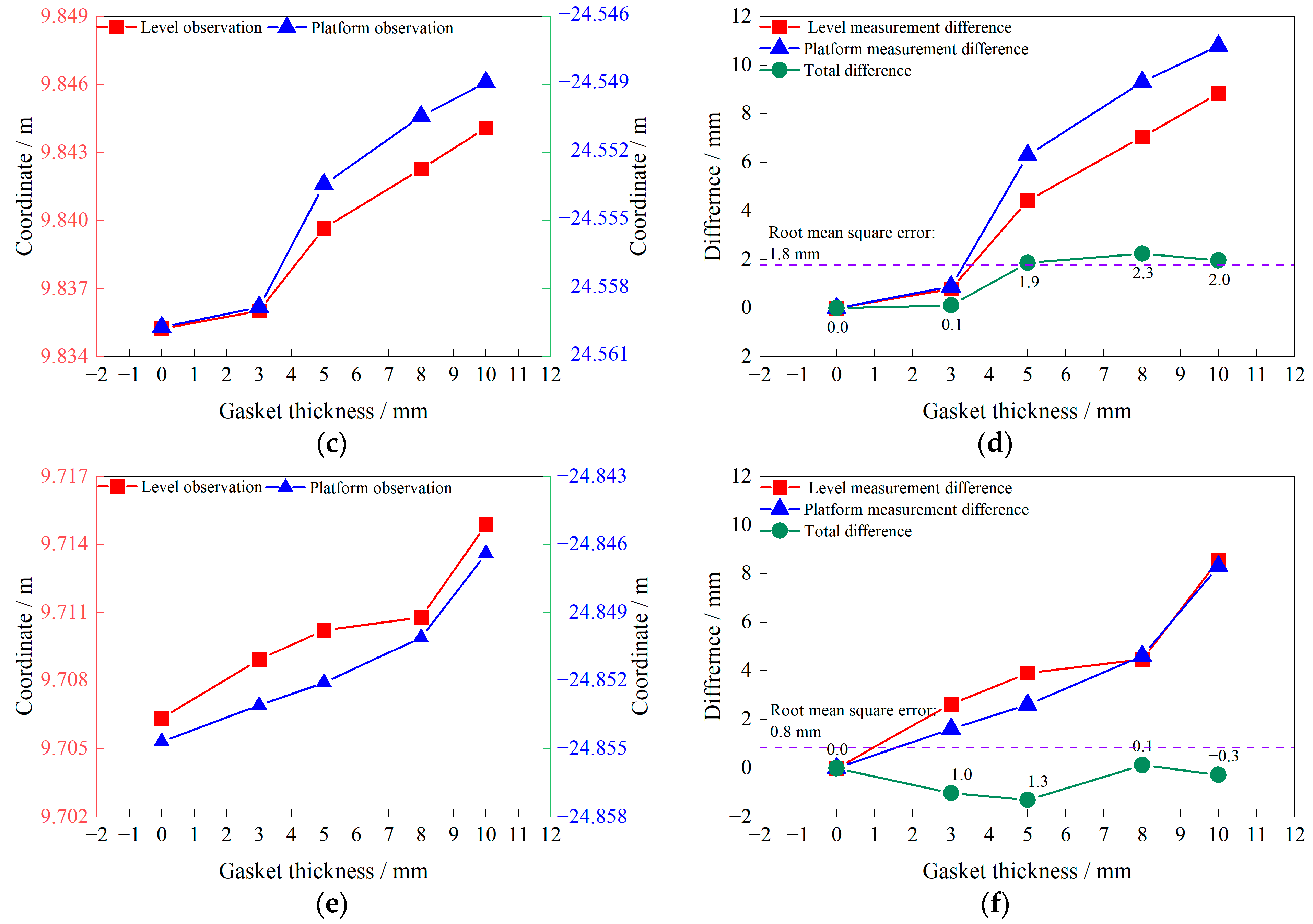
3.2. RLMD-SVD Joint Denoising Method

The time frame for data collection in this experiment was from 3 December 2021 to 20 January 2022, resulting in measurement point data for the five locations in Figure 3a. The BDS monitoring point receiver used the double-difference correction information of the reference station with the solution method in this paper, using the real-time kinematic differential algorithm to obtain real-time kinematic coordinates and sending the data every five minutes. The GNSS monitoring point displacements of the five measurement points after the BeiDou solution are shown in Figure 5.

The displacement changes of the GNSS monitoring points usually refer to the coordinate changes. When a monitoring point undergoes displacement, its position coordinates will change, which is usually expressed by the change of east coordinates, north coordinates, and up coordinates. As can be seen from Figure 5a–e, because of on-site monitoring equipment and solar power failures during engineering application, the equipment sometimes suffered from an insufficient power supply time or even power failure. It resulted in insufficient or even zero satellite epoch data being collected by the BDS equipment in a single day in the late monitoring period of the BDT2 measurement point, failing to achieve high-precision positioning results. The overall trend in changes in the deformation curves of the remaining monitoring points was relatively gentle and the cumulative deformations were small and fluctuated within a specific range, indicating that the ground deformation along the subway was essentially stable during the monitoring period. By comparing and analyzing the fluctuation ranges of the deformation curves of the monitoring points, it was evident that the eastward displacements of each measurement point from BDT1 to BDT5 had smaller vibration amplitudes, fluctuating in the range of 0–1.0 mm, except for BDT1, which fluctuated between 0 and 2.0 mm. The northward displacements of the BDT1–BDT5 measurement points fluctuated between −2.0 mm and +2.0 mm, except for a few points that exceeded 6.0 mm. The up coordinates of the BDT1–BDT5 measurement points fluctuated between −2.0 mm and 0 mm, except for the BDT1 and BDT3 displacements, which more often fluctuated between −4.0 mm and 0 mm. The remaining three points fluctuated between −2.0 mm and 0 mm. Of the five measurement points, BDT1 was located on the side of the road and was most affected by traffic, leading to large fluctuations in the observation data and a reduction in its quality, which mainly affected the accuracy of the observation results in the horizontal direction. In general, the horizontal observation accuracy meets the requirements for ground deformation monitoring.

The GNSS tangential angle process line variation of the BDT2 measurement point on 5 February 2022 and the GNSS daily variation rate of the process line are shown in Figure 6.

The GNSS tangential angle diagram refers to the image obtained by adding the clock difference of the receiver and the clock difference of the satellite into the position equation to obtain the corrected position coordinates in the GNSS positioning calculation. The GNSS tangential angle process line variation and daily variation rate can assist monitoring personnel in assessing deformation conditions. Figure 6 shows that the GNSS tangential angle of the BDT2 measurement point had the same trend in the east and north, fluctuating between −90° and +90°, and the up tangential angle mainly fluctuated between −60° and +60°. The deformation rate of the plane and the vertical deformation of the measurement points were basically the same, fluctuating over 0–6.0 mm/d. It indicates that the deformation of BDT2 is basically stable during the monitoring periods. The deformation trend changed abruptly in the later stage of monitoring due to equipment failure.

The monitoring data for 3 December 2021 through to 6 January 2022 are shown in

Table 1. Ground deformation monitoring along the subway line.

Ground Deformation Monitoring along Subway Line
Measurement Point	Horizontal Displacement			Vertical Displacement
	Cumulative Displacement (mm)		Cumulative Horizontal Displacement (mm)	Cumulative Displacement Rate (mm/d)	Cumulative Settlement (mm)	Cumulative Settlement Rate (mm/d)
	Δx	Δy	ΔHr	ΔHr/d	Δh	Δh/d
BDT1	−2.7	1.0	2.9	0.09	−5.1	−0.15
BDT2	No data	No data	No data	No data	No data	No data
BDT3	−1.0	0	1.0	0.03	−4.8	−0.14
BDT4	−1.5	0.9	1.7	0.05	−3.2	−0.09
BDT5	−1.1	0.4	1.2	0.04	−3.0	−0.09

, where it is evident that BDT2 had no data due to system failure. BDT1 was close to the road with heavy traffic and the horizontal and vertical displacements were larger, with values of −2.7 mm and −5.1 mm, respectively. BDT3 was similar to the BDT1 measurement point and had a consistent cumulative settlement with a difference of 5.88% and a cumulative settlement rate of −0.15 mm/d; the cumulative settlement rates of BDT4 and BDT5 were −0.14 mm/d and −0.09 mm/d. The cumulative horizontal displacement values of BDT3–BDT5 were similar and the cumulative displacement rates were all less than 0.15 mm/d.

The RLMD method was used to pre-denoise the eastward displacement curve of the GNSS data for each measurement point; the SVD method was then used to post-denoise it. In the SVD method, the number of singular values is determined in advance. If too few singular values are selected, the signal appears over-decomposed, resulting in the loss of useful signals. If too many singular values are selected, the signal appears under-decomposed, resulting in incomplete noise elimination. The GNSS monitoring signals of the ground deformation of the subway were mainly composed of three parts: the actual structural vibration, the multipath error, and random noise. Therefore, the number of singular values was set to six. The displacements of various measurement points after denoising with SVD, RLMD, and RLMD-SVD are shown in Figure 7.

As is shown in Figure 7, although the SVD and RLMD methods alone provided some noise reduction for the original signal, the RLMD–SVD joint method had strong robustness and good noise reduction. The maximum fluctuation value of BDT1 decreased by 45%, from 4.0 to 2.2; the minimum fluctuation value increased from −1.7 to 1.7; and the displacement curve fluctuated steadily over 0–2.0 mm. For the BDT2 observation data, the maximum fluctuation value decreased by 53%, from 1.7 to 0.8; the minimum fluctuation value increased from −1.4 to −1.0; and the displacement curve fluctuated between −1.0 mm and 1.0 mm. The maximum fluctuation value of BDT3 decreased by 80%, from 2.0 to 0.4; the minimum fluctuation value increased from −1.4 to −0.5; and the displacement curve fluctuated steadily between −0.5 mm and 0.5 mm. The maximum BDT4 fluctuation value decreased by 83%, from 2.4 to 0.4; the minimum fluctuation value increased from −0.7 to −0.6; and the displacement curve fluctuated steadily between −0.6 mm and 0.5 mm. The BDT5 maximum fluctuation value decreased from 2.8 to 0.4, representing an 86% decrease; the minimum fluctuation value increased from −1.0 to −0.4 mm; and the displacement curve fluctuated steadily between −1 mm and 0.5 mm. In summary, based on the RLMD–SVD joint denoising method, the maximum magnitude of each measurement point was reduced by a maximum of 86% and the eastward displacement of each measurement point fluctuated stably between −1.0 mm and 1.0 mm, providing better error correction of the BDS signals with high accuracy.

An experiment was conducted to investigate the static relative positioning accuracy of the deformation monitoring system. The test simulated the ground deformation by a given amount using a three-dimensional displacement platform. The experiment consisted of two parts: RTK positioning accuracy and static relative positioning accuracy. A Tianbao electronic level meter DINI03 (main characteristics: 1 km round trip accuracy: 0.3 mm; measuring range: 1.5–100 m; compensation accuracy: ±15′; leveling accuracy: ±0.2″; telescope magnification: 32×; 100 m field of view: 2.8 m; short-sight distance: 0.6 m; night and tunnel measurements are possible) and a three-axis fine-tuning platform were used to verify the vertical and horizontal displacements of three BDS receiving stations (BDT1–BDT3). The monitoring accuracy was based on the deformation monitoring level and accuracy requirements stipulated in the Engineering Measurement Standard [44] and the second-grade level measurement was selected.

The BDT1 measurement point was selected for two-way static relative positioning accuracy testing according to the optimal observation period, initially testing a specified displacement (coordinate position) of 3 mm and moving 6, 8, 11, and 13 mm. Based on the moving coordinates of the 3D precision displacement stage, the initial coordinates are set for different working conditions: 21 December 2022, 3 mm initial coordinates: East 235.4914 m, North 744.0885 m, Up −25.6737 m; 22 December 2022, 3 mm initial coordinates: East 1035.5862 m, North 1576.289 m, Up −25.3263 m; 24 December 2022, 3 mm initial coordinates: East 1105.0611 m, North 1676.05 m, Up −25.2136 m.

For comparison, the change curves of the east, north, and up displacements of the BDT1 precision leveling at different times are shown in Figure 8, based on the initial December 21 coordinates. The movement offset of the 3D precision displacement platform and the data differences between the 3D precision displacement platform and the ground deformation monitoring system are shown in Figure 9.

According to the experimental results shown in Figure 8a–c, it can be observed that the measurements of precision leveling in one direction fluctuate within a small range for different gasket thicknesses, which indicates that the thickness of the gaskets has a minimal impact on the measurement results of precision leveling. It shows that the precision leveling is highly stable and capable of accurately detecting changes in the leveling.

The experimental results obtained from the three-dimensional precision displacement platform and the ground deformation monitoring system, as illustrated in Figure 9a–c, demonstrate a significant agreement between the measurement results of the monitoring system and the precision leveling. The comparison is made considering the given displacement of the three-dimensional precision displacement platform at various time intervals. The maximum deviation of the measurement results of the monitoring system from the precision leveling measurements is 1.3 mm and the minimum is −0.1 mm, both of which are smaller than 1.5 mm. This indicates that the monitoring system has a high positioning accuracy. Taking the precision-level measurement value as the relative true value, on 21 December, 22 December, and 24 December, the horizontal displacement observation values of the deformation monitoring system calculated from the BDT1 measurement point were close to the precision-level measurement value, meeting the accuracy requirement.

The observation accuracy of the ground deformation monitoring system was directly evaluated using the root mean square error (RMSE), calculated as:

$$e=\sqrt{\frac{{{\displaystyle \sum }}_1^{n}d\times d}{n}}$$

(25)

$$d=\left|S_b-S_d\right|$$

(26)

where d is the displacement difference. The smaller the value of $e$, the higher the accuracy of the monitoring system.

RMSE is a statistical measure of the differences between observed values and it is used to evaluate the observation accuracy of the ground deformation monitoring system. Calculated from Equations (25) and (26), the RMSE of the horizontal displacement observations and precision-level measurements were 1.0 mm, 1.0 mm, and 0.5 mm. The cumulative RMSE of the three-day data deviation was 1.1 mm and the trend in the GNSS elevation observation results was consistent with the synchronized precision-level measurement results.

To test the accuracy of ground settlement vertical displacement along the subway, three measurement points, BDT1, BDT2, and BDT3, were selected and five different gasket thicknesses of 0, 3, 5, 8, and 10 mm were used to simulate the changes in height. The precision leveling and the deformation monitoring system were used to synchronously measure the vertical displacements to monitor abnormal ground settlement conditions along the subway. The testing was performed from 09:30 on 17 October 2022 to 19:49 on 18 October 2022 and the vertical displacement of measurement points BDT1-BDT3 is shown in Figure 10.

As is seen in Figure 10, the measured vertical displacement deviations of the platforms for the BDT1, BDT2, and BDT3 measurement points from the precision-level measurements range from −1.5 mm to +2.7 mm, +0.1 mm to +2.3 mm, and −1.3 mm to +0.1 mm, respectively. The plane displacement deviations ranged from −1.3 mm to +0.7 mm, +0.4 mm to +1.3 mm, and +0.1 mm to +1.0 mm. For the BDT1 measurement point with a 10 mm gasket thickness, the maximum deviation value was 2.7 mm. For the BDT2 measurement point with a 3 mm gasket thickness, the minimum deviation value was 0.1 mm.

When the precision leveling values were taken as the relative true values for each measurement point, the observed static relative positioning settlement of the BDS was smaller than that of the precision leveling readings. The RMSE of the vertical displacement deviation for the BDT1, BDT2, and BDT3 measurement points were 1.3 mm, 1.8 mm, and 0.8 mm, respectively. The cumulative RMSE of each measurement point was 1.5 mm and the trend in the GNSS height observation results was consistent with the simultaneous precision leveling survey results.

In summary, the ground deformation monitoring system has a vertical positioning accuracy that is better than 2.7 mm and a horizontal positioning accuracy that is better than 1.3 mm. Both the horizontal and vertical positioning accuracies meet the requirements. Under the same observation period and baseline length, the horizontal observation accuracy of the system is better than the vertical observation accuracy.

Based on the GNSS monitoring data after noise reduction, it has been demonstrated that a ground deformation monitoring system can be constructed along the subway to provide statistical information for structures, measurement points, and equipment. It can display site monitoring point coordinate position information relative to the reference point and recent ground deformation data changes and establish the corresponding threshold. Different levels of alarm information can be set according to the threshold value size when the monitoring data exceed the threshold value to effectively monitor the ground deformation along the subway and provide risk analysis control and early warnings.

4. Discussion

The ground deformation monitoring system used in this study has advantages, such as convenience and automation, compared to the traditional engineering observation methods. Lee et al. [7] used a fixed GNSS monitoring station located on the embankment of New Wanjin Road and compared the GNSS monitoring station data with those obtained via the D-InSAR technique to obtain an accurate ground deformation RMSE value of 0.7 mm. Xiao et al. [22] established GNSS in the Shuangwangcheng Reservoir, an important regulation project in the eastern route of the South-to-North Water Diversion Project. The global positioning system (GPS) and the deformation monitoring system accuracies for different observation periods were evaluated and the results showed that the deformation monitoring system performance is comparable to the GPS, especially for longer observation period solutions, with daily solution accuracies of 1 mm horizontally and 2 mm vertically. The above-mentioned GNSS is consistent with the experimental accuracy of the measured results in this study. The two observation methods can reflect the subway’s ground deformation characteristics. However, the traditional level observation method adopts manual observation, which is greatly affected by the environment and other factors and cannot be observed under weather conditions such as rainfall, wind, and fog, which significantly impact the completeness of the observation data. The deformation monitoring system provides 24-hour automated continuous observation, ensuring the integrity of the observation data, and its deformation time curve is continuous and smoother to monitor the ground deformation along the subway more effectively.

The noise of the monitoring data can be effectively reduced by the RLMD–SVD joint denoising method. Figure 7 compares the real-time processing data of the BDT1–BDT5 measurement points based on the RLMD–SVD joint denoising methods and the RLMD and SVD methods. The RLMD–SVD joint denoising method can provide more effective noise reduction in the GNSS monitoring data than the RLMD or SVD noise-reduction methods alone. Zhu et al. [45] reported the elimination of multipath errors in satellite signals using a smooth wavelet transform. They simplified the random noise into a Gaussian white noise model combined with autocorrelation function noise determination quasi-measurement and empirical modal decomposition noise-reduction methods to reduce the random noise components in the signals. The algorithmically corrected real-time acquisition of the ground deformation monitoring system signals with the precision leveling measurements between the error was less than 1 mm. Based on the RLMD–SVD joint denoising method in this paper, the two studies agree on the deformation monitoring trend. Therefore, the RLMD–SVD joint denoising method applied to GNSS engineering applications can eliminate satellite signal errors, improve observation accuracy, and meet accuracy requirements.

The localization accuracy of the deformation monitoring system based on the RLMD–SVD joint denoising method has been effectively improved. The experimental results in Figure 10 show that the vertical positioning accuracy of the ground deformation monitoring system was greater than 2.7 mm, the horizontal positioning accuracy was greater than 1.3 mm, and the measurement error was less than 1.5 mm. The measured and precision-leveled BDT1, BDT2, and BDT3 measurement point vertical displacement deviations of the platforms ranged from −1.5 mm to +2.7 mm, +0.1 mm to +2.3 mm, and −1.3 mm to +0.1 mm, respectively; furthermore, the plane displacement deviations ranged from −1.3 mm to +0.7 mm, +0.4 mm to +1.3 mm, and +0.1 mm to +1.0 mm, respectively. For a 10 mm gasket thickness, the maximum BDT1 measurement point deviation value was 2.7 mm; for a 3 mm gasket thickness, the minimum BDT2 was at least 0.1 mm. When the precision leveling values were taken as the relative true values of each measuring point, the observed static relative positioning settlement of the BDS was smaller than that of the precision leveling readings. The RMSE of the BDT1, BDT2, and BDT3 measurement point vertical displacement deviations were 1.3 mm, 1.8 mm, and 0.8 mm, respectively. The cumulative RMSE of each measurement point was 1.5 mm.

5. Conclusions

A BDS observation point was set up to monitor ground deformation along the subway line in real time. The ground deformation monitoring system signal noise was reduced by using the RLMD–SVD joint denoising method and the ground deformation monitoring system for subway structure safety was constructed. The system has achieved effective monitoring of ground deformation. The method was validated by experimental comparisons with the traditional precision leveling. The following conclusions were obtained:

(1)

A ground deformation monitoring system for subway structure safety based on the GNSS was established. Compared to traditional engineering observation methods, the system has achieved the convenience and automated monitoring of surface deformation;

(2)

The ground deformation monitoring system makes up for the shortcomings of the traditional method; however, due to the influence of environmental noise and other factors, it will produce a certain degree of error. A RLMD–SVD joint denoising method is proposed. The ground deformation monitoring system noise-reduction results show that up to 86% of the noise in the data can be reduced. Using the RLMD–SVD joint denoising method more effectively eliminates the noise in the ground deformation monitoring system signal compared to the SVD and RLMD methods alone;

(3)

The RLMD–SVD joint denoising method improves the horizontal and vertical localization accuracy of the ground deformation monitoring system. The vertical positioning accuracy of the deformation monitoring system was greater than 2.7 mm, the horizontal positioning accuracy was greater than 1.3 mm, and the measurement error was less than 1.5 mm, meeting the ground deformation observation technical requirements of a subway structure. It provides a new method for ground deformation monitoring.

References

1. Lazarus, D. Structural engineering for the Elizabeth line: Damage Assessment and Monitoring for Buildings on the Elizabeth Line. Struct. Eng. J. Inst. Struct. Eng. 2018, 96, 14–24. [Google Scholar] [CrossRef]
2. Torp-Petersen, G.E.; Black, M.G. Geotechnical Investigation and Assessment of Potential Building Damage Arising from Ground Movements: CrossRail. Proc. Inst. Civ. Eng.-Transport. 2001, 147, 107–119. [Google Scholar] [CrossRef]
3. Szabo, B.; Brzeski, J.; González Martí, J. Use of Linked Monitoring Systems for Asset Protection at Finsbury Circus during SCL Tunnelling for Crossrail Station. In Crossrail Project: Infrastructure Design and Construction; ICE Publishing: London, UK, 2015; pp. 315–345. [Google Scholar] [CrossRef]
4. Korff, M.; Kaalberg, F. Monitoring Dataset of Deformations Related to Deep Excavations for North-South Line in Amsterdam. In Geotechnical Aspects of Underground Construction in Soft Ground; Korean Geotechnical Society: Seoul, Republic of Korea, 2014; pp. 321–326. [Google Scholar] [CrossRef]
5. Schiess, S.; Berget, G.E.; Arnesen, P.; Brunes, M.T.; Seter, H.; Muggerud, A.M.F. GNSS Technology for Precise Positioning in CCAM: A Comparative Evaluation of Services. IEEE Access 2023, 11, 47816–47826. [Google Scholar] [CrossRef]
6. Yu, W.; Peng, H.; Pan, L.; Dai, W.; Qu, X.; Ren, Z. Performance Assessment of High-Rate GPS/BDS Precise Point Positioning for Vibration Monitoring Based on Shaking Table Tests. Adv. Space Res. 2022, 69, 2362–2375. [Google Scholar] [CrossRef]
7. Lee, J.; Lee, W.; Lee, H.; Yoon, H. The Settlement Analysis of the Saemenguem Coastal Area by the Tide Using D-InSAR. J. Coast. Res. 2019, 91, 361. [Google Scholar] [CrossRef]
8. Bovenga, F.; Nitti, D.O.; Fornaro, G.; Radicioni, F.; Stoppini, A.; Brigante, R. Using C/X-Band SAR Interferometry and GNSS Measurements for the Assisi Landslide Analysis. Int. J. Remote Sens. 2013, 34, 4083–4104. [Google Scholar] [CrossRef]
9. Adamcová, D.; Bartoň, S.; Osinski, P.; Pasternak, G.; Podlasek, A.; Vaverková, M.D.; Koda, E. Analytical Modelling of MSW Landfill Surface Displacement Based on GNSS Monitoring. Sensors 2020, 20, 5998. [Google Scholar] [CrossRef] [PubMed]
10. Iwahana, G.; Busey, R.; Saito, K. Seasonal and Interannual Ground-Surface Displacement in Intact and Disturbed Tundra along the Dalton Highway on the North Slope, Alaska. Land 2020, 10, 22. [Google Scholar] [CrossRef]
11. Kyriou, A.; Kakavas, M.; Nikolakopoulos, K.G.; Koukouvelas, I.; Stefanopoulos, P.; Zygouri, V.; Tsigalidas, D. Landslide Mapping and Volume Estimation Using UAV-Based Point Clouds, GIS and Geophysical Techniques. In Proceedings of the Earth Resources and Environmental Remote Sensing/GIS Applications XI, Online, 21–25 September 2020; Volume 11534, pp. 171–180. [Google Scholar] [CrossRef]
12. Bayik, C.; Abdikan, S.; Ozdemir, A.; Arıkan, M.; Balik Sanli, F.; Dogan, U. Investigation of the Landslides in Beylikdüzü-Esenyurt Districts of Istanbul from InSAR and GNSS Observations. Nat. Hazards 2021, 109, 1201–1220. [Google Scholar] [CrossRef]
13. Lu, D.; Tan, J.; Cai, B.; Liu, J.; Wang, J. GNSS Signal in Railway Train Operation Scenario Quality Grid Generation Method. In Proceedings of the ION Pacific PNT—ION 2019 Pacific PNT Meeting, Honolulu, HI, USA, 8–11 April 2019; pp. 529–539. [Google Scholar] [CrossRef]
14. Mi, L. Research on Construction of Urban Rail First-Order Control Network in Extra Large Area. Surv. Mapp. Geol. Miner. Resour. Surv. Mapp. Geol. Miner. Resour. 2013, 29, 8–10. [Google Scholar] [CrossRef]
15. Guang, Y. High Precision First-Grade Control Network Survey for Guangzhou Rail Transit. Eng. Surv. Mapp. Eng. Surv. Mapp. 2012, 21, 82–85. [Google Scholar] [CrossRef]
16. Peternel, T.; Janža, M.; Šegina, E.; Bezak, N.; Maček, M. Recognition of Landslide Triggering Mechanisms and Dynamics Using GNSS, UAV Photogrammetry and In Situ Monitoring Data. Remote Sens. 2022, 14, 3277. [Google Scholar] [CrossRef]
17. Evers, M.; Kyriou, A.; Schulz, K.; Nikolakopoulos, K.G. A Study on Recent Ground Deformation near Patras, Greece. In Proceedings of the Earth Resources and Environmental Remote Sensing/GIS Applications X, Strasbourg, France, 10–12 September 2019; Volume 11560, pp. 108–119. [Google Scholar] [CrossRef]
18. Gokceoglu, C.; Kocaman, S.; Nefeslioglu, H.A.; Ok, A.O. Use of Multisensor and Multitemporal Geospatial Datasets to Extract the Foundation Characteristics of a Large Building: A Case Study. Bull. Eng. Geol. Environ. 2021, 80, 3251–3269. [Google Scholar] [CrossRef]
19. Chen, M.; Lv, P.; Nie, W.; Tan, C.; Bai, Z.; Liao, Y.; Zhou, J. The Role of Water and Lithology on the Deformation and Failure of an Anaclinal Rock Slope in a Hydropower Reservoir. Adv. Civ. Eng. 2020, 8852227. [Google Scholar] [CrossRef]
20. Peng, Y.; Dong, D.; Chen, W.; Zhang, C. Stable Regional Reference Frame for Reclaimed Land Subsidence Study in East China. Remote Sens. 2022, 14, 3984. [Google Scholar] [CrossRef]
21. Xiao, R.; Shi, H.; He, X.; Li, Z.; Jia, D.; Yang, Z. Deformation Monitoring of Reservoir Dams Using GNSS: An Application to South-to-North Water Diversion Project, China. IEEE Access 2019, 7, 54981–54992. [Google Scholar] [CrossRef]
22. Zhu, S.; Zuo, X.; Shi, K.; Li, Y.; Guo, S.; Li, C. Surface Subsidence Monitoring in Kunming City with Time-Series InSAR and GNSS. Appl. Sci. 2022, 12, 12752. [Google Scholar] [CrossRef]
23. Du, Q.; Li, G.; Zhou, Y.; Chai, M.; Chen, D.; Qi, S.; Wu, G. Deformation Monitoring in an Alpine Mining Area in the Tianshan Mountains Based on SBAS-InSAR Technology. Adv. Mater. Sci. Eng. 2021, 9988017. [Google Scholar] [CrossRef]
24. Li, R.; Li, Z.; Han, J.; Lu, P.; Qiao, G.; Meng, X.; Hao, T.; Zhou, F. Monitoring Surface Deformation of Permafrost in Wudaoliang Region, Qinghai–Tibet Plateau with ENVISAT ASAR Data. Int. J. Appl. Earth Obs. Geoinf. 2021, 104, 102527. [Google Scholar] [CrossRef]
25. Luo, L.; Ma, W.; Zhang, Z.; Zhuang, Y.; Yang, J.; Cao, X.; Liang, S.; Yi, S. Integration of Terrestrial Laser Scanning and Soil Sensors for Deformation and Hydrothermal Monitoring of Frost Mounds. Measurement 2019, 131, 513–523. [Google Scholar] [CrossRef]
26. Palano, M.; Pezzo, G.; Serpelloni, E.; Devoti, R.; D’Agostino, N.; Gandolfi, S.; Sparacino, F.; Anderlini, L.; Poluzzi, L.; Tavasci, L.; et al. Geopositioning Time Series from Offshore Platforms in the Adriatic Sea. Sci. Data 2020, 7, 373. [Google Scholar] [CrossRef] [PubMed]
27. Aytekin, G.; Topan, H.; Elkar, Y.E.; Kisi, M.; Erisik, O. 2D Orientation Accuracy of Güktürk-1 Panchromatic Imagery. In Proceedings of the 2019 9th International Conference on Recent Advances in Space Technologies (RAST 2019), Istanbul, Turkey, 11–14 June 2019; pp. 821–826. [Google Scholar] [CrossRef]
28. Usmanov, B.M.; Gainullin, I.; Gafurov, A.M.; Rudenko, K.A.; Ivanov, M.A. Using Multitemporal Remote Sensing Data for Evaluation of the Kuibyshev Reservoir Bank Transformation (Laishevo and Ostolopovo Archaeological Sites, Tatarstan, Russia). In Proceedings of the Earth Resources and Environmental Remote Sensing/GIS Applications XII, Online, 13–17 September 2021; Volume 11863, pp. 100–110. [Google Scholar] [CrossRef]
29. Vieira, G.; Mora, C.; Pina, P.; Ramalho, R.; Fernandes, R. UAV-Based Very High Resolution Point Cloud, Digital Surface Model and Orthomosaic of the Chã Das Caldeiras Lava Fields (Fogo, Cabo Verde). Earth Syst. Sci. Data 2021, 13, 3179–3201. [Google Scholar] [CrossRef]
30. Shahmoradi, J.; Talebi, E.; Roghanchi, P.; Hassanalian, M. A Comprehensive Review of Applications of Drone Technology in the Mining Industry. Drones 2020, 4, 34. [Google Scholar] [CrossRef]
31. Mainsant, G.; Larose, E.; Brönnimann, C.; Jongmans, D.; Michoud, C.; Jaboyedoff, M. Ambient Seismic Noise Monitoring of a Clay Landslide: Toward Failure Prediction. J. Geophys. Res. Earth Surf. 2012, 117, F1. [Google Scholar] [CrossRef]
32. Moschas, F.; Psimoulis, P.A.; Stiros, S.C. GPS/RTS Data Fusion to Overcome Signal Deficiencies in Certain Bridge Dynamic Monitoring Projects. Smart Struct. Syst. 2013, 12, 251–269. [Google Scholar] [CrossRef]
33. Penzias, A.A.; Wilson, R.W. A Measurement of Excess Antenna Temperature at 4080-Mc/s. Astrophys. J. 1965, 142, 419. [Google Scholar] [CrossRef]
34. Blewitt, G. An Automatic Editing Algorithm for GPS Data. Geophys. Res. Lett. 1990, 17, 199–202. [Google Scholar] [CrossRef]
35. Zhu, H.; Li, J.; Wang, C.; Xu, A.; Gao, M. A method of BeiDou navigation satellite system double difference network real-time kinematic. Sci. Surv. Mappin 2017, 42, 1–6. [Google Scholar] [CrossRef]
36. Hu, G.; Cui, W. Observation Random Model of Precision Positioning with Combined GPS/GLONASS. J. Remote Sens. 2001, 5, 95–99. [Google Scholar]
37. Xiong, C.; Lu, H.; Zhu, J.; Yu, J. Dynamic deformation monitoring of bridge structures based on GPS-RTK and accelerometers. J. Vib. Shock. 2019, 38, 69. [Google Scholar] [CrossRef]
38. Smith, J.S. The Local Mean Decomposition and Its Application to EEG Perception Data. J. R. Soc. Interface 2005, 2, 443–454. [Google Scholar] [CrossRef] [PubMed]
39. Liu, Z.; Jin, Y.; Zuo, M.J.; Feng, Z. Time-Frequency Representation Based on Robust Local Mean Decomposition for Multicomponent AM-FM Signal Analysis. Mech. Syst. Signal Process. 2017, 95, 468–487. [Google Scholar] [CrossRef]
40. Cai, J.; Xiao, Y. Bearing Fault Diagnosis Method Based on the Generalized S Transform Time–Frequency Spectrum de-Noised by Singular Value Decomposition. Proc. Inst. Mech. Eng. Part C J. Mech. Eng. Sci. 2019, 233, 2467–2477. [Google Scholar] [CrossRef]
41. He, X.; Gao, Z.; Xiao, R.; Luo, H.; Jia, D.; Zhang, Z. Current status and outlook of the research on surface deformation monitoring by the integrated method of InSAR and Beidou/GNSS. J. Surv. Mapp. 2022, 51, 1338–1355. (In Chinese) [Google Scholar]
42. Li, B.; Ge, Y. Single Epoch GPS Deformation Monitoring Data Processing and System Development. J. Henan Polytech. Univ. (Nat. Sci. Ed.). 2007, 26, 165–170. [Google Scholar] [CrossRef]
43. Chen, X.; Yang, Y.; Zhou, C.; Liao, C. Study on Fast Positioning Algorithm for BeiDou Post-Mission Network RTK. IOP Conf. Ser. Mater. Sci. Eng. 2020, 780, 032051. [Google Scholar] [CrossRef]
44. China Nonferrous Metals Industry Association (CNMIA). Ministry of Housing and Urban-Rural Development of the People’s Republic of China; General Administration of State Market Supervision and Administration; Engineering Measurement Standard; CNMIA: Beijing, China, 2020. [Google Scholar]
45. Zhu, Y.; Shuang, M.; Sun, D.; Guo, H. Algorithm and Application of Foundation Displacement Monitoring of Railway Cable Bridges Based on Satellite Observation Data. Appl. Sci. 2023, 13, 2868. [Google Scholar] [CrossRef]
Figure 1. Measurement point arrangement in the study area.
Buildings 13 02682 g001
Figure 2. Block diagram of the ground deformation monitoring system along the subway line.
Buildings 13 02682 g002
Figure 3. Monitoring station equipment and station locations. (a) BDS monitoring equipment; (b) Location of measurement stations.
Buildings 13 02682 g003
Figure 4. Installation of measurement points and reference stations. (a) Measurement station; (b) CORS reference station.
Buildings 13 02682 g004
Figure 5. Real-time coordinates of each measurement point after BeiDou solutions. (a) BDT1 measurement point; (b) BDT2 measurement point; (c) BDT3 measurement point; (d) BDT4 measurement point; (e) BDT5 measurement point.
Buildings 13 02682 g005aBuildings 13 02682 g005b
Figure 6. The GNSS tangential angle process line variation and daily variation rate of the process line at the BDT2 measurement point. (a) GNSS tangential angle process line variation; (b) Daily variation rate of the process line.
Buildings 13 02682 g006
Figure 7. Displacement curves of each measurement point after noise reduction. (a) BDT1 measurement point; (b) BDT2 measurement point; (c) BDT3 measurement point; (d) BDT4 measurement point; (e) BDT5 measurement point.
Buildings 13 02682 g007
Figure 8. Displacement of measurement points over different periods. (a) Up displacement; (b) East displacement; (c) North displacement.
Buildings 13 02682 g008
Figure 9. Displacement deviation of the BDT1 measurement point over different periods. (a) Displacement on 21 December; (b) Displacement on 22 December; (c) Displacement on 24 December.
Buildings 13 02682 g009
Figure 10. Comparison of vertical displacements at each measurement point. (a) BDT1 measurement point value; (b) BDT1 measurement point difference; (c) BDT2 measurement point value; (d) BDT2 measurement point difference; (e) BDT3 measurement point value; (f) BDT3 measurement point difference.
Buildings 13 02682 g010aBuildings 13 02682 g010b