
Hilbert-Huang Transform-Based Seismic Intensity Parameters for Performance-Based Design of RC-Framed Structures

Abstract
:1. Introduction
2. Methods
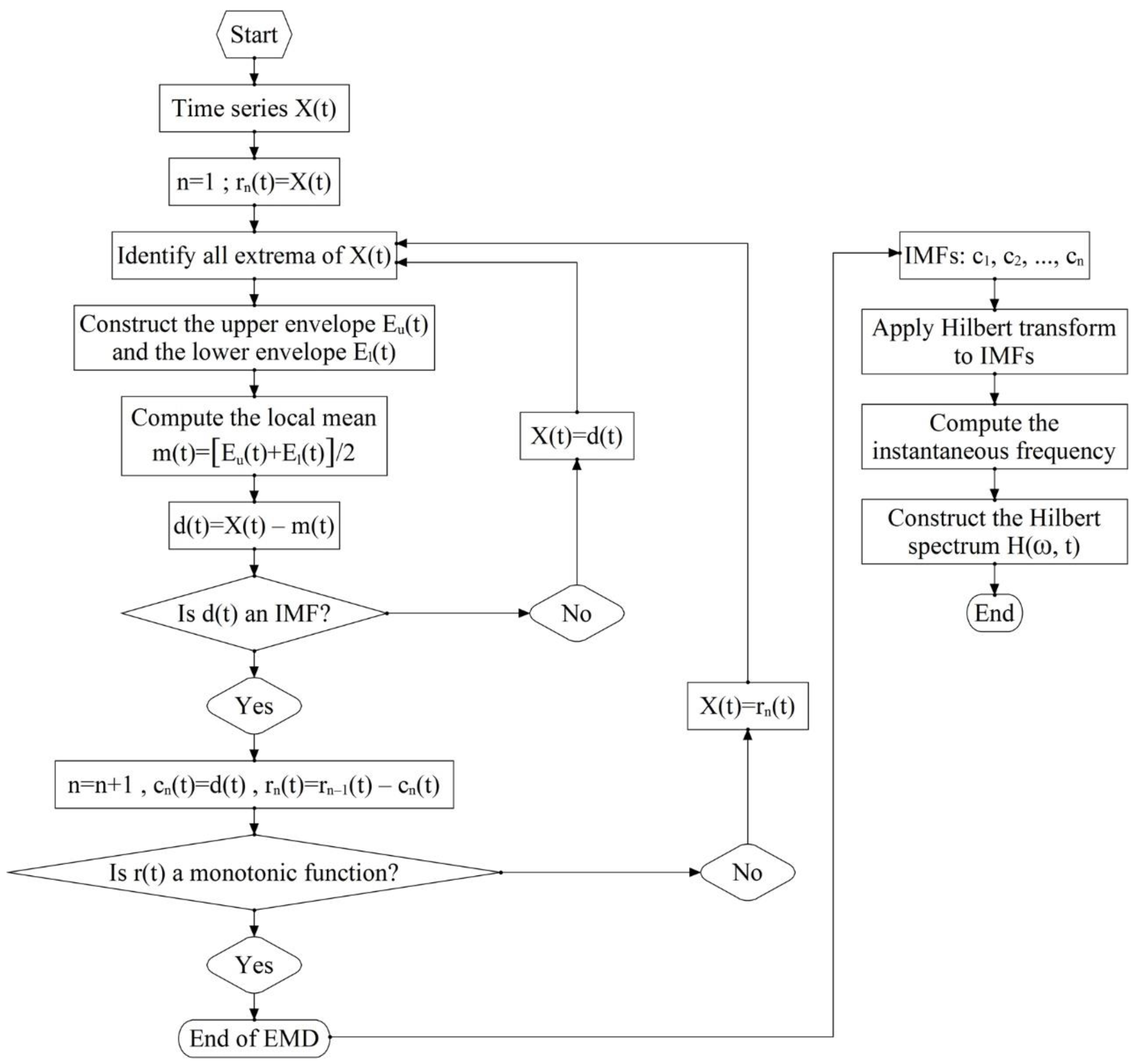
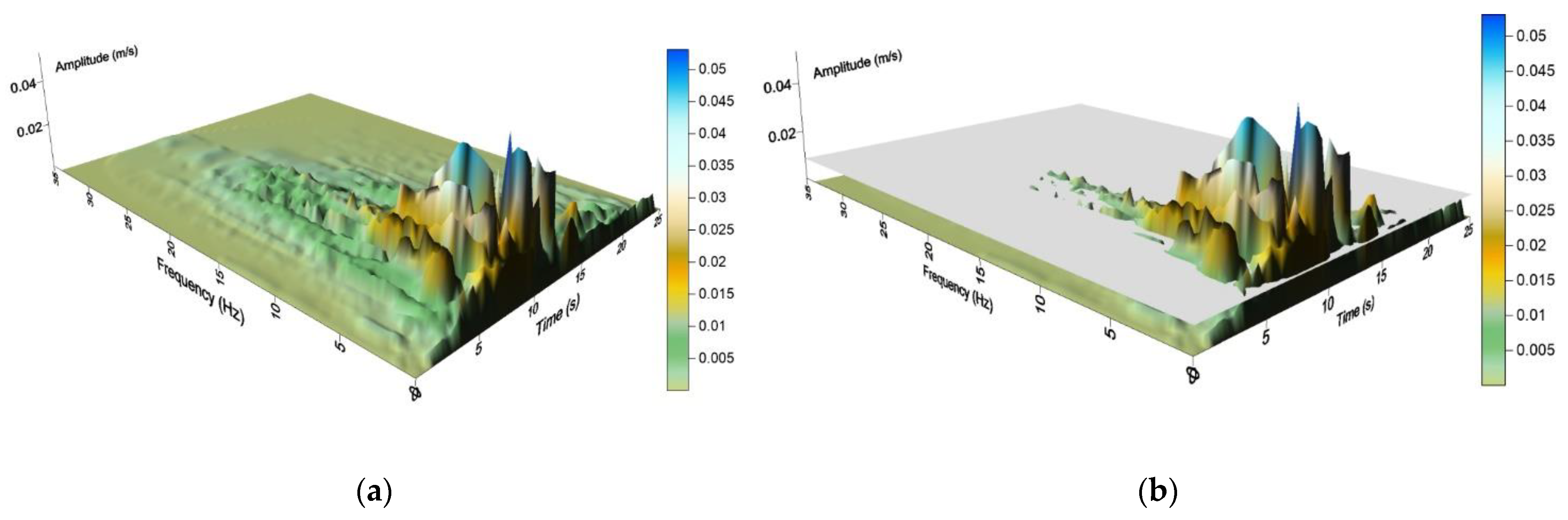
2.1. Hilbert-Huang Transform (HHT) Analysis
2.2. HHT-Based Seismic Parameters
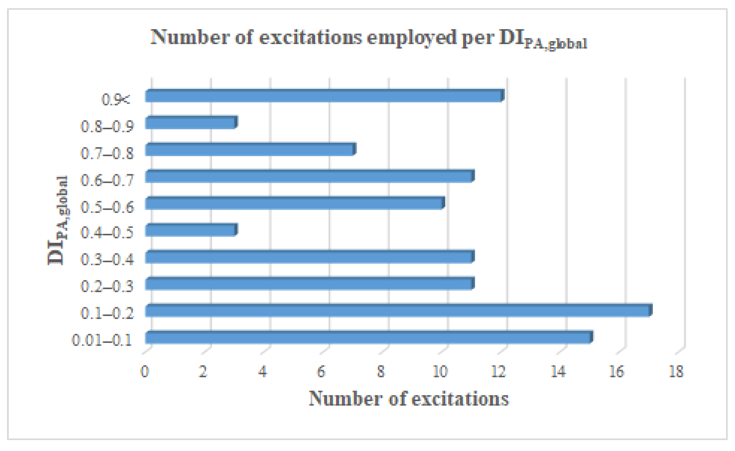
2.3. Global Damage Index of Park and Ang
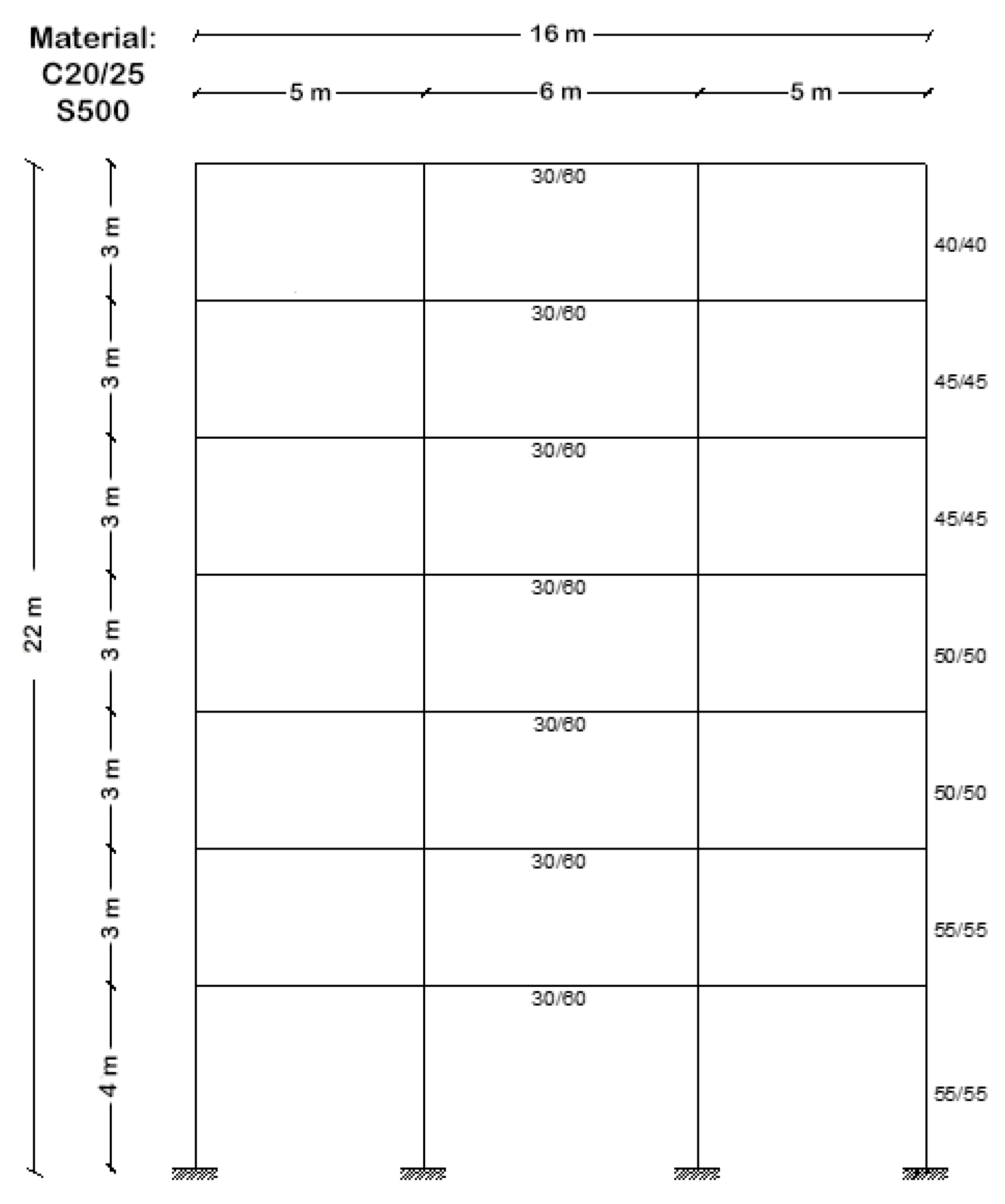
3. Application
4. Results
4.1. Evaluation of the HHT-Based Seismic Intensity Parameters
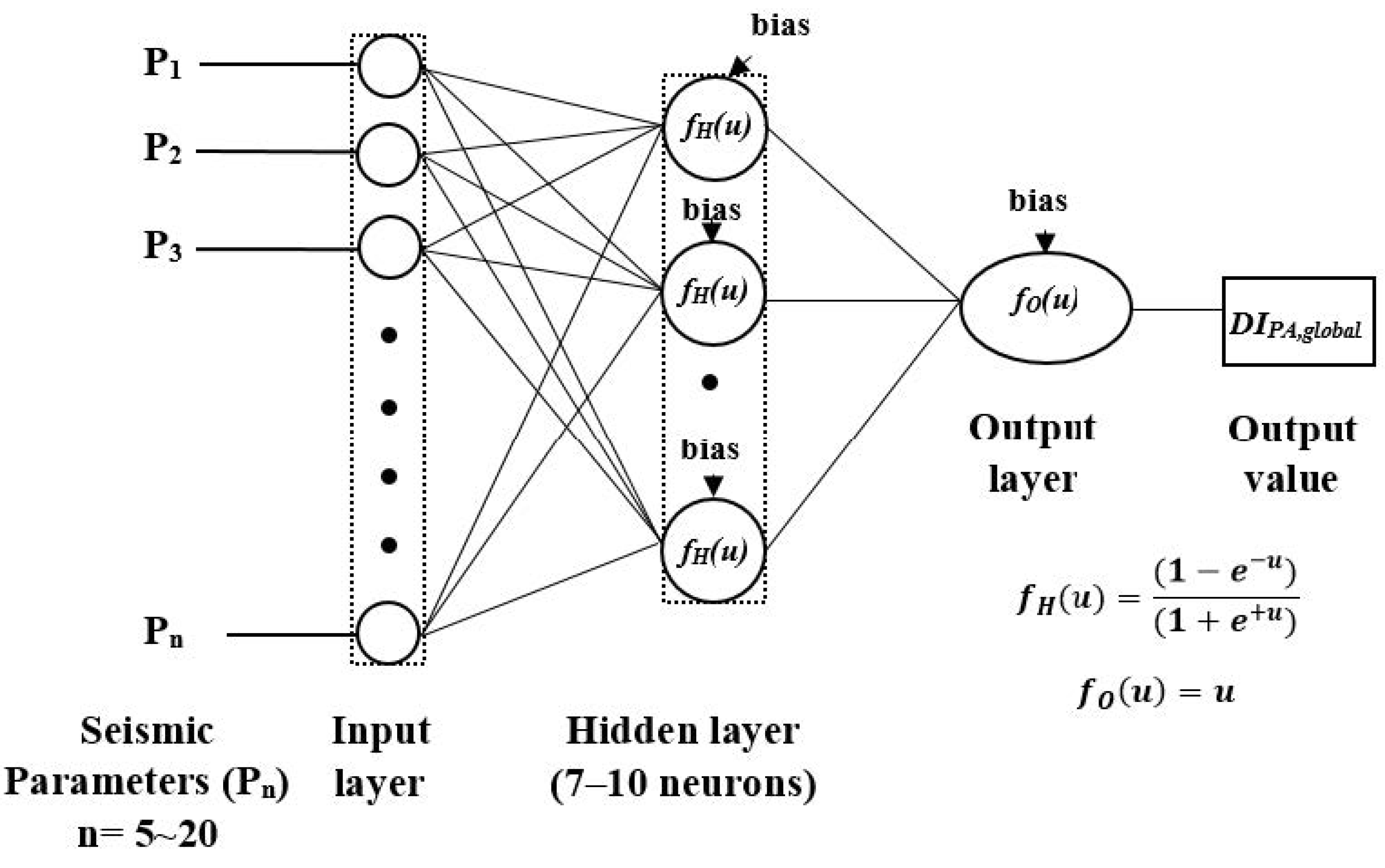
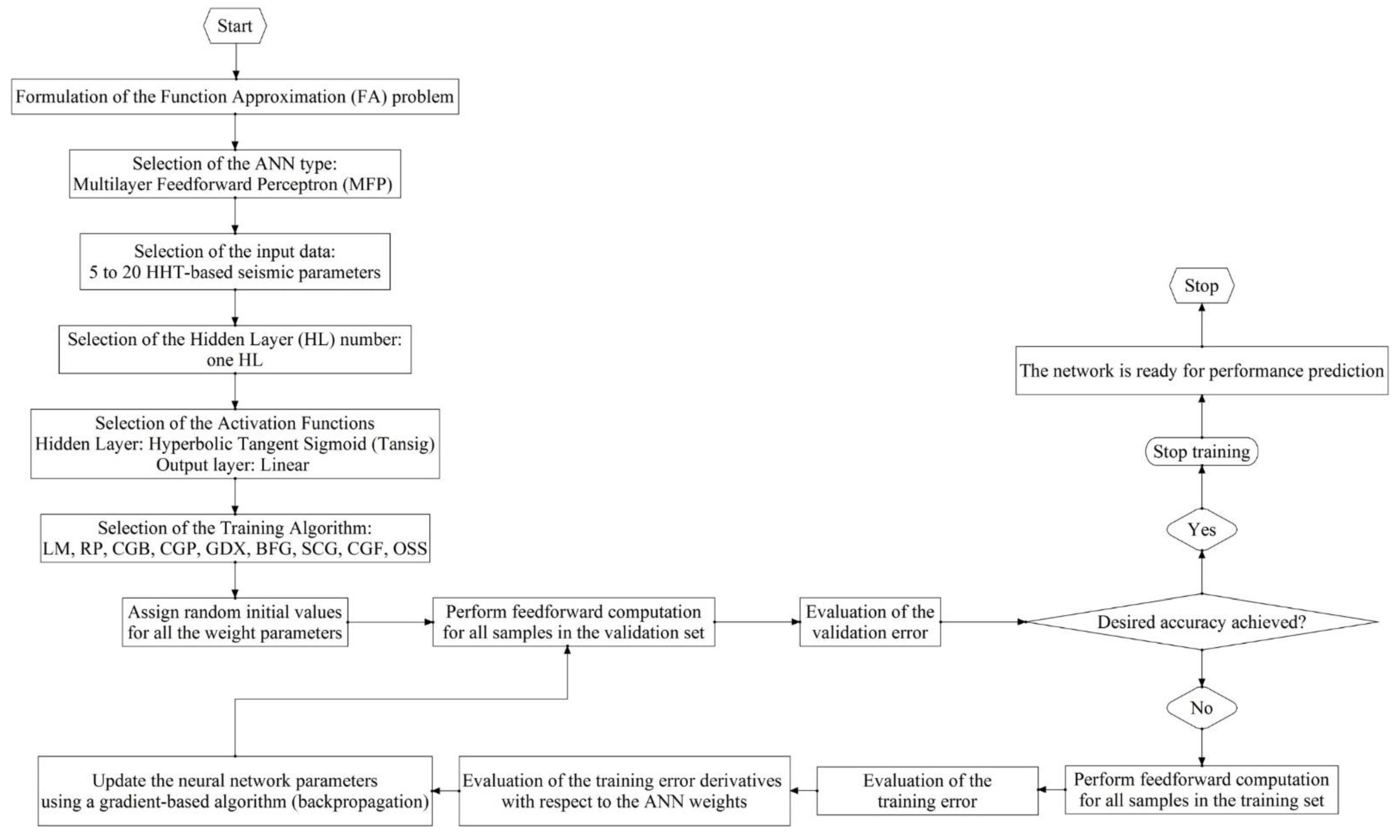
4.2. Problem Formulation and ANN Framework Selection
4.3. Configuration of ANNs
4.4. Calculation of ANNs
5. Discussion
6. Conclusions
Author Contributions
Funding
Institutional Review Board Statement
Informed Consent Statement
Data Availability Statement
Conflicts of Interest
References
- Elenas, A. Correlation between seismic acceleration parameters and overall structural damage indices of buildings. Soil Dyn. Earthq. Eng. 2000, 20, 93–100. [Google Scholar] [CrossRef]
- Elenas, A.; Meskouris, K. Correlation study between seismic acceleration parameters and damage indices of structures. Eng. Struct. 2001, 23, 698–704. [Google Scholar] [CrossRef]
- Alvanitopoulos, P.F.; Andreadis, I.; Elenas, A. A genetic algorithm for the classification of earthquake damages in buildings. In Proceedings of the 5th IFIP Conference on Artificial Intelligence Applications & Innovations, Thessaloniki, Greece, 23–25 April 2009; pp. 341–346. [Google Scholar]
- Alvanitopoulos, P.F.; Andreadis, I.; Elenas, A. A New Algorithm for the Classification of Earthquake Damages in Structures. In Proceedings of the 5th IASTED Conference on Signal Processing, Pattern Recognition and Applications, Innsbruck, Austria, 13–15 February 2008; pp. 151–156. [Google Scholar]
- Alvanitopoulos, P.F.; Andreadis, I.; Elenas, A. Neuro-fuzzy techniques for the classification of earthquake damages in buildings. Measurement 2010, 43, 797–809. [Google Scholar] [CrossRef]
- Elenas, A. Seismic-Parameter-Based Statistical Procedure for the Approximate Assessment of Structural Damage. Math. Probl. Eng. 2014, 2014, 916820. [Google Scholar] [CrossRef]
- Elenas, A. Interdependency between seismic acceleration parameters and the behavior of structures. Soil Dyn. Earthq. Eng. 1997, 16, 317–322. [Google Scholar] [CrossRef]
- Nanos, N.; Elenas, A.; Ponterosso, P. Correlation of different strong motion duration parameters and damage indicators of reinforced concrete structures. In Proceedings of the 14th World Conference on Earthquake Engineering, Beijing, China, 12–17 October 2008. [Google Scholar]
- Kostinakis, K.; Athanatopoulou, A.; Morfidis, K. Correlation between ground motion intensity measures and seismic damage of 3D R/C buildings. Eng. Struct. 2015, 82, 151–167. [Google Scholar] [CrossRef]
- Tyrtaiou, M.; Elenas, A. Seismic Damage Potential Described by Intensity Parameters Based on Hilbert-Huang Transform Analysis and Fundamental Frequency of Structures. Earthq. Struct. 2020, 18, 507–517. [Google Scholar]
- Tyrtaiou, M.; Elenas, A. Novel Hilbert spectrum-based seismic intensity parameters interrelated with structural damage. Earthq. Struct. 2019, 16, 197–208. [Google Scholar]
- Lautour, O.R.; Omenzetter, P. Prediction of seismic-induced structural damage using artificial neural networks. Eng. Struct. 2009, 31, 600–606. [Google Scholar] [CrossRef]
- Morfidis, K.; Kostinakis, K. Approaches to the rapid seismic damage prediction of r/c buildings using artificial neural networks. Eng. Struct. 2018, 165, 120–141. [Google Scholar] [CrossRef]
- Tsou, P.; Shen, M.H. Structural Damage Detection and Identification Using Neural Network. In Proceedings of the 34thAIAA/ASME/ASCEAHS/ASC, Structural, Structural Dynamics and Materials Conference, AIAA/ASME Adaptive Structural Forum, La Jolla, CA, USA, 19–22 April 1993. [Google Scholar]
- Wu, X.; Ghaboussi, J.; Garrett, J. Use of Neural Network in Detection of Structural Damage. Comput. Struct. 1992, 42, 649–659. [Google Scholar] [CrossRef]
- Zhao, J.; Ivan, J.N.; DeWold, J.T. Structural Damage Detection Using Artificial Neural Networks. J. Infrastructural Syst. 1998, 13, 182–189. [Google Scholar] [CrossRef]
- Zameeruddin, M.; Sangle, K.K. Damage assessment of reinforced concrete moment resisting frames using performance-based seismic evaluation procedure. J. King Saud Univ. Eng. Sci. 2021, 33, 227–239. [Google Scholar] [CrossRef]
- Zameeruddin, M.; Sangle, K.K. Review on Recent developments in the performance-based seismic design of reinforced concrete structures. Structures 2016, 6, 119–133. [Google Scholar] [CrossRef]
- Loh, C.H.; Chao, S.H. The Use of Damage Function in Performanced-Based Seismic Design of Structures. In Proceedings of the 13th World Conference on Earthquake Engineering, Vancouver, BC, Canada, 1–6 August 2004. [Google Scholar]
- Gholizadeh, S.; Fattahi, F. Damage-controlled performance-based design optimization of steel moment frames. Struct. Des. Tall Spec. Build. 2018, 27, e1498. [Google Scholar] [CrossRef]
- Jiang, H.J.; Chen, L.Z.; Chen, Q. Seismic Damage Assessment and Performance Levels of Reinforced Concrete Members. In Proceedings of the 12th East Asia-Pacific Conference on Structural Engineering and Construction, Hong Kong, China, 26–28 January 2011. [Google Scholar]
- Huang, N.; Shen, Z.; Long, S.R.; Wu, M.C.; Shih, H.H.; Zheng, Q.; Yen, N.; Tung, C.C.; Liu, H.H. The empirical mode decomposition and the Hilbert spectrum for nonlinear and non-stationary time series analysis. Proc. R. Soc. Lond. A Math. Phys. Eng. Sci. 1998, 454, 903–995. [Google Scholar] [CrossRef]
- Huang, N.; Shen, Z.; Long, S.R. A new view of nonlinear water waves: The Hilbert spectrum. Annu. Rev. Fluid Mech. 1999, 31, 417–457. [Google Scholar] [CrossRef]
- Huang, N.; Wu, M.L.; Qu, W.; Long, S.; Shen, S. Applications of Hilbert–Huang transform to non-stationary financial time series analysis applied stochastic models in business and industry. Appl. Stoch. Models Bus. Ind. 2003, 19, 245–268. [Google Scholar] [CrossRef]
- Yu, M.; Erlei, Y.; Bin, R.; Haiyang, Z.; Xiaohong, L. Improved Hilbert spectral representation method and its application to seismic analysis of shield tunnel subjected to spatially correlated ground motions. Soil Dyn. Earthq. Eng. 2018, 111, 119–130. [Google Scholar]
- Zhang, R.R.; Ma, S.; Safak, E.; Hartzell, S. Hilbert–Huang transform analysis of dynamic and earthquake motion recordings. ASCE J. Eng. Mech. 2003, 129, 861–875. [Google Scholar] [CrossRef]
- Park, Y.J.; Ang, A.H.-S. Mechanistic seismic damage model for reinforced concrete. J. Struct. Eng. 1985, 111, 722–739. [Google Scholar] [CrossRef]
- Park, Y.J.; Ang, A.H.-S.; Wen, Y.K. Damage-limiting aseismic design of buildings. Earthq. Spectra 1987, 3, 1–26. [Google Scholar] [CrossRef]
- Kunnath, S.K.; Reinhorn, A.M.; Abel, J.F. A Computational Tool for Seismic Performance of Reinforced Concrete Building. Comput. Struct. 1992, 41, 157–173. [Google Scholar] [CrossRef]
- Kunnath, S.K.; Reinhorn, A.M.; Lobo, R.F. IDARC Version 3.0: A Program for the Inelastic Damage Analysis of Reinforced Concrete Structures, Report No. NCEER-92-0022; National Center for Earthquake Engineering Research; University at Buffalo: Buffalo, NY, USA, 1992. [Google Scholar]
- Eurocode 8. Design of Structures for Earthquake Resistance—Part 1: General Rules, Seismic Actions, and Rules for Buildings; European Committee for Standardization: Brussels, Belgium, 2004. [Google Scholar]
- Eurocode 2. Design of Concrete Structures—Part 1: General Rules and Rules for Building; European Committee for Standardization: Brussels, Belgium, 2000. [Google Scholar]
- Reinhorn, A.M.; Roh, H.; Sivaselvan, M.; Kunnath, S.K.; Valles, R.E.; Madan, A.; Li, C.; Lobo, R.; Park, Y.J. IDARC2D Version 7.0: A Program for the Inelastic Damage Analysis of Structures; Tech. Rep. MCEER-09-0006; MCEER, State University of New York at Buffalo: Buffalo, NY, USA, 2009. [Google Scholar]
- Gholamreza, G.A.; Elham, R. Maximum damage prediction for regular reinforced concrete frames under consecutive earthquakes. Earthq. Struct. 2018, 14, 129–142. [Google Scholar]
- The Math Works Inc. MATLAB and Statistics Toolbox Release 2016b; The Math Works Inc.: Natick, MA, USA, 2016. [Google Scholar]


| Structural | Structural Damage Degree | |||
|---|---|---|---|---|
| Damage Index | Low | Medium | Large | Total |
| DIPA,global | ≤0.3 | 0.3 < DIPA,global ≤ 0.6 | 0.6 < DIPA,global ≤ 0.8 | DIPA,global > 0.80 |
| Parameters | Statistics | |||
|---|---|---|---|---|
| Min Value | Max Value | Average | Standard Deviation | |
| S1(HHT) (-) | 153.5914 | 4946.3096 | 1350.4544 | 1077.2957 |
| V1(HHT) (m/s) | 0.2050 | 27.8891 | 5.1527 | 4.8203 |
| V1(Pos,HHT) (m/s) | 0.0597 | 7.4880 | 1.5228 | 1.5227 |
| S1(Pos,HHT) (-) | 5.8971 | 548.5377 | 86.5171 | 95.3434 |
| A1(max,HHT) (m/s) | 0.0114 | 0.8559 | 0.2363 | 0.1848 |
| A1(mean,HHT) (m/s) | 0.0005 | 0.1044 | 0.0212 | 0.0200 |
| A1(dif,HHT) (m/s) | 0.0104 | 0.7850 | 0.2151 | 0.1707 |
| A1(Pos,HHT) (m/s) | 0.0016 | 0.1115 | 0.0247 | 0.0196 |
| VA1(mean) (m2/s2) | 0.0002 | 1.1788 | 0.1243 | 0.1637 |
| VA1(max) (m2/s2) | 0.0054 | 7.5185 | 1.4392 | 1.6682 |
| VA1(dif,HHT) (m2/s2) | 0.0053 | 7.1969 | 1.3150 | 1.5428 |
| V2(HHT) (m/s) | 0.0000 | 2.1061 | 0.2515 | 0.3048 |
| S2(HHT) (-) | 0.0024 | 33.9103 | 12.8771 | 9.7173 |
| V2(Pos,HHT) (m/s) | 0.0000 | 0.5207 | 0.1024 | 0.1009 |
| S2(Pos,HHT) (-) | 0.0012 | 14.8652 | 4.0702 | 3.2751 |
| A2(max,HHT) (m/s) | 0.0074 | 0.7622 | 0.1567 | 0.1526 |
| A2(mean,HHT) (m/s) | 0.0006 | 0.2554 | 0.0287 | 0.0456 |
| SEF(HHT) (-) | 0.0237 | 10.0491 | 1.2100 | 1.4582 |
| A3(max,HHT) (m/s) | 0.0056 | 0.7422 | 0.1410 | 0.1380 |
| A3(mean,HHT) (m/s) | 0.0006 | 0.2559 | 0.0292 | 0.0460 |
| A1(Ratio,HHT) (-) | 0.0125 | 0.2241 | 0.0946 | 0.0483 |
| A2(Ratio,HHT) (-) | 0.0339 | 0.4424 | 0.1748 | 0.1040 |
| A3(Ratio,HHT) (-) | 0.0358 | 0.4957 | 0.1950 | 0.1119 |
| A1(HHT) (m/s) | 0.0001 | 0.0259 | 0.0055 | 0.0052 |
| A2(HHT) (m/s) | 0.0006 | 0.2157 | 0.0275 | 0.0407 |
| A2(Pos,HHT) (m/s) | 0.0009 | 0.1490 | 0.0295 | 0.0266 |
| SEFA1(mean) (m/s) | 0.0000 | 0.3947 | 0.0343 | 0.0614 |
| SEFA2(mean) (m/s) | 0.0000 | 2.5669 | 0.0862 | 0.3145 |
| SEFA3(mean) (m/s) | 0.0000 | 2.5718 | 0.0871 | 0.3149 |
| SEFA1(max) (m/s) | 0.0006 | 3.0521 | 0.3912 | 0.6208 |
| SEFA2(max) (m/s) | 0.0002 | 7.6594 | 0.3452 | 0.8981 |
| SEFA3(max) (m/s) | 0.0002 | 7.4580 | 0.3188 | 0.8620 |
| S1A3(max) (m/s) | 3.2803 | 1193.1771 | 172.0672 | 212.8759 |
| S1A1(mean) (m/s) | 0.5230 | 121.8580 | 21.4915 | 21.1580 |
| S1A3(mean) (m/s) | 0.7957 | 350.8138 | 27.3436 | 43.0174 |
| S2A2(mean) (m/s) | 0.0000 | 2.4942 | 0.2603 | 0.3402 |
| A2(dif,HHT) (m/s) | 0.0044 | 0.5721 | 0.1280 | 0.1208 |
| VA2(dif,HHT) (m2/s2) | 0.0000 | 1.0673 | 0.0538 | 0.1251 |
| VA2(mean) (m2/s2) | 0.0000 | 0.5380 | 0.0180 | 0.0660 |
| VA2(max) (m2/s2) | 0.0000 | 1.6053 | 0.0719 | 0.1880 |
| Backpropagation (BP) Training Algorithms | |
|---|---|
| Levenberg–Marquardt (LM) | Powell–Beale conjugate gradient (CGB) |
| BFGS quasi-Newton (BFG) | Fletcher–Powell conjugate gradient (CGF) |
| Resilient backpropagation (RP) | Polak–Ribiere conjugate gradient (CGP) |
| Scaled conjugate gradient (BP) | One step secant (OSS) |
| Gradient descent with momentum and adaptive linear (GDX) | |
| Group 1—R Statistics | ||||||||
|---|---|---|---|---|---|---|---|---|
| Training Algorithm | 7-Neuron Hidden Layer | 8-Neuron Hidden Layer | ||||||
| Min | Max | Mean | st.dev. | Min | Max | Mean | st.dev. | |
| trainlm | −0.6317 | 0.9841 | 0.9042 | 0.0514 | −0.5746 | 0.9882 | 0.9028 | 0.0528 |
| trainbfg | −0.7944 | 0.9642 | 0.8435 | 0.1083 | −0.7071 | 0.9616 | 0.8459 | 0.1013 |
| trainrp | −0.7916 | 0.9601 | 0.8173 | 0.1193 | −0.7038 | 0.9610 | 0.8182 | 0.1168 |
| trainscg | −0.8194 | 0.9618 | 0.8376 | 0.1149 | −0.5916 | 0.9610 | 0.8391 | 0.1075 |
| traincgb | −0.6282 | 0.9700 | 0.8524 | 0.1051 | −0.6858 | 0.9633 | 0.8530 | 0.1004 |
| traincgf | −0.7216 | 0.9626 | 0.8393 | 0.1123 | −0.5956 | 0.9616 | 0.8432 | 0.1048 |
| traincgp | −0.6849 | 0.9681 | 0.8410 | 0.1111 | −0.6858 | 0.9618 | 0.8416 | 0.1060 |
| trainoss | −0.6953 | 0.9551 | 0.8346 | 0.1127 | −0.6866 | 0.9587 | 0.8366 | 0.1052 |
| traingdx | −0.8512 | 0.9529 | 0.5966 | 0.3801 | −0.8566 | 0.9490 | 0.5958 | 0.3822 |
| 9-Neuron Hidden Layer | 10-Neuron Hidden Layer | |||||||
| min | max | mean | st.dev. | min | max | mean | st.dev. | |
| trainlm | −0.6315 | 0.9861 | 0.9017 | 0.0537 | −0.5106 | 0.9838 | 0.9008 | 0.0548 |
| trainbfg | −0.6329 | 0.9622 | 0.8479 | 0.0956 | −0.6748 | 0.9674 | 0.8495 | 0.0918 |
| trainrp | −0.6880 | 0.9571 | 0.8191 | 0.1150 | −0.7202 | 0.9622 | 0.8191 | 0.1147 |
| trainscg | −0.7171 | 0.9721 | 0.8398 | 0.1032 | −0.6387 | 0.9656 | 0.8403 | 0.1005 |
| traincgb | −0.6102 | 0.9661 | 0.8536 | 0.0963 | −0.6650 | 0.9692 | 0.8538 | 0.0937 |
| traincgf | −0.7120 | 0.9618 | 0.8455 | 0.1000 | −0.6384 | 0.9627 | 0.8470 | 0.0963 |
| traincgp | −0.6248 | 0.9616 | 0.8420 | 0.1017 | −0.6650 | 0.9658 | 0.8423 | 0.0990 |
| trainoss | −0.7067 | 0.9607 | 0.8379 | 0.0994 | −0.6939 | 0.9584 | 0.8386 | 0.0959 |
| traingdx | −0.8554 | 0.9524 | 0.5910 | 0.3853 | −0.8609 | 0.9512 | 0.5829 | 0.3904 |
| Group 1—MSE Statistics | ||||||||
|---|---|---|---|---|---|---|---|---|
| Training Algorithm | 7-Neuron Hidden Layer | 8-Neuron Hidden Layer | ||||||
| Min | Max | Mean | st.dev. | Min | Max | Mean | st.dev. | |
| trainlm | 0.0029 | 0.3214 | 0.0183 | 0.0103 | 0.0023 | 0.3745 | 0.0187 | 0.0107 |
| trainbfg | 0.0066 | 0.4275 | 0.0266 | 0.0154 | 0.0070 | 0.4322 | 0.0264 | 0.0149 |
| trainrp | 0.0072 | 0.5305 | 0.0309 | 0.0180 | 0.0071 | 0.5626 | 0.0309 | 0.0182 |
| trainscg | 0.0069 | 0.5355 | 0.0272 | 0.0156 | 0.0070 | 0.4774 | 0.0271 | 0.0151 |
| traincgb | 0.0054 | 0.3952 | 0.0249 | 0.0146 | 0.0067 | 0.4553 | 0.0249 | 0.0143 |
| traincgf | 0.0067 | 0.5486 | 0.0270 | 0.0155 | 0.0070 | 0.5340 | 0.0265 | 0.0149 |
| traincgp | 0.0058 | 0.4636 | 0.0267 | 0.0153 | 0.0070 | 0.4553 | 0.0267 | 0.0150 |
| trainoss | 0.0081 | 0.4828 | 0.0280 | 0.0158 | 0.0074 | 0.4388 | 0.0279 | 0.0153 |
| traingdx | 0.0084 | 0.7099 | 0.0595 | 0.0534 | 0.0091 | 1.0021 | 0.0618 | 0.0579 |
| 9-Neuron Hidden Layer | 10-Neuron Hidden Layer | |||||||
| min | max | mean | st.dev. | min | max | mean | st.dev. | |
| trainlm | 0.0026 | 0.4003 | 0.0190 | 0.0110 | 0.0030 | 0.4343 | 0.0192 | 0.0114 |
| trainbfg | 0.0069 | 0.4309 | 0.0262 | 0.0145 | 0.0059 | 0.4576 | 0.0260 | 0.0141 |
| trainrp | 0.0077 | 0.9272 | 0.0309 | 0.0183 | 0.0069 | 0.6747 | 0.0310 | 0.0187 |
| trainscg | 0.0050 | 0.6328 | 0.0271 | 0.0148 | 0.0062 | 0.7438 | 0.0271 | 0.0148 |
| traincgb | 0.0062 | 0.4318 | 0.0249 | 0.0141 | 0.0056 | 0.6200 | 0.0249 | 0.0140 |
| traincgf | 0.0069 | 0.4737 | 0.0262 | 0.0146 | 0.0068 | 0.5245 | 0.0260 | 0.0144 |
| traincgp | 0.0069 | 0.4597 | 0.0267 | 0.0147 | 0.0062 | 0.6200 | 0.0268 | 0.0147 |
| trainoss | 0.0071 | 0.5018 | 0.0278 | 0.0149 | 0.0075 | 0.6408 | 0.0277 | 0.0147 |
| traingdx | 0.0086 | 0.9054 | 0.0648 | 0.0626 | 0.0087 | 0.9933 | 0.0685 | 0.0677 |
| Group 2—R Statistics | ||||||||
|---|---|---|---|---|---|---|---|---|
| Training Algorithm | 7-Neuron Hidden Layer | 8-Neuron Hidden Layer | ||||||
| Min | Max | Mean | st.dev. | Min | Max | Mean | st.dev. | |
| trainlm | −0.7834 | 0.9730 | 0.8824 | 0.0494 | −0.8028 | 0.9706 | 0.8818 | 0.0502 |
| trainbfg | −0.7816 | 0.9357 | 0.8439 | 0.0594 | −0.7483 | 0.9396 | 0.8443 | 0.0590 |
| trainrp | −0.7842 | 0.9248 | 0.8305 | 0.0692 | −0.7366 | 0.9312 | 0.8298 | 0.0709 |
| trainscg | −0.7808 | 0.9317 | 0.8399 | 0.0655 | −0.7462 | 0.9397 | 0.8394 | 0.0657 |
| traincgb | −0.7319 | 0.9450 | 0.8475 | 0.0604 | −0.8165 | 0.9441 | 0.8474 | 0.0607 |
| traincgf | −0.7618 | 0.9350 | 0.8431 | 0.0640 | −0.7744 | 0.9364 | 0.8433 | 0.0640 |
| traincgp | −0.7618 | 0.9350 | 0.8420 | 0.0629 | −0.7661 | 0.9327 | 0.8415 | 0.0636 |
| trainoss | −0.7750 | 0.9289 | 0.8397 | 0.0607 | −0.8062 | 0.9312 | 0.8396 | 0.0598 |
| traingdx | −0.8783 | 0.9161 | 0.6750 | 0.3145 | −0.8764 | 0.9184 | 0.6622 | 0.3236 |
| 9-Neuron Hidden Layer | 10-Neuron Hidden Layer | |||||||
| min | max | mean | st.dev. | min | max | mean | st.dev. | |
| trainlm | −0.7400 | 0.9698 | 0.8812 | 0.0513 | −0.7718 | 0.9668 | 0.8807 | 0.0519 |
| trainbfg | −0.8010 | 0.9400 | 0.8444 | 0.0595 | −0.6828 | 0.9406 | 0.8445 | 0.0595 |
| trainrp | −0.7421 | 0.9271 | 0.8286 | 0.0735 | −0.7388 | 0.9299 | 0.8275 | 0.0756 |
| trainscg | −0.7310 | 0.9326 | 0.8387 | 0.0662 | −0.7900 | 0.9337 | 0.8377 | 0.0680 |
| traincgb | −0.7702 | 0.9417 | 0.8469 | 0.0618 | −0.7683 | 0.9428 | 0.8463 | 0.0626 |
| traincgf | −0.8038 | 0.9417 | 0.8429 | 0.0655 | −0.7986 | 0.9383 | 0.8426 | 0.0663 |
| traincgp | −0.7792 | 0.9351 | 0.8409 | 0.0640 | −0.7785 | 0.9394 | 0.8403 | 0.0649 |
| trainoss | −0.7717 | 0.9373 | 0.8391 | 0.0601 | −0.7550 | 0.9388 | 0.8385 | 0.0602 |
| traingdx | −0.8769 | 0.9152 | 0.6483 | 0.3341 | −0.8766 | 0.9224 | 0.6326 | 0.3464 |
| Group 2—MSE Statistics | ||||||||
|---|---|---|---|---|---|---|---|---|
| Training Algorithm | 7-Neuron Hidden Layer | 8-Neuron Hidden Layer | ||||||
| Min | Max | Mean | st.dev. | Min | Max | Mean | st.dev. | |
| trainlm | 0.0049 | 0.3890 | 0.0225 | 0.0113 | 0.0055 | 0.6813 | 0.0228 | 0.0119 |
| trainbfg | 0.0115 | 0.6292 | 0.0272 | 0.0097 | 0.0108 | 0.6749 | 0.0273 | 0.0100 |
| trainrp | 0.0134 | 0.4977 | 0.0298 | 0.0117 | 0.0122 | 0.4258 | 0.0300 | 0.0122 |
| trainscg | 0.0122 | 0.3255 | 0.0276 | 0.0100 | 0.0109 | 0.6220 | 0.0278 | 0.0104 |
| traincgb | 0.0099 | 0.3728 | 0.0263 | 0.0093 | 0.0100 | 0.4400 | 0.0264 | 0.0096 |
| traincgf | 0.0116 | 0.3831 | 0.0270 | 0.0098 | 0.0113 | 0.4416 | 0.0270 | 0.0100 |
| traincgp | 0.0119 | 0.3452 | 0.0272 | 0.0096 | 0.0119 | 0.4335 | 0.0274 | 0.0099 |
| trainoss | 0.0126 | 0.5109 | 0.0280 | 0.0099 | 0.0122 | 0.7328 | 0.0281 | 0.0100 |
| traingdx | 0.0149 | 1.0202 | 0.0500 | 0.0407 | 0.0144 | 1.3593 | 0.0529 | 0.0446 |
| 9-Neuron Hidden Layer | 10-Neuron Hidden Layer | |||||||
| min | max | mean | st.dev. | min | max | mean | st.dev. | |
| trainlm | 0.0055 | 0.4265 | 0.0230 | 0.0124 | 0.0060 | 0.5154 | 0.0233 | 0.0129 |
| trainbfg | 0.0107 | 0.4202 | 0.0273 | 0.0102 | 0.0106 | 6.7141 | 0.0274 | 0.0124 |
| trainrp | 0.0129 | 0.4869 | 0.0303 | 0.0129 | 0.0124 | 0.3849 | 0.0306 | 0.0135 |
| trainscg | 0.0119 | 0.3476 | 0.0280 | 0.0107 | 0.0119 | 0.4225 | 0.0282 | 0.0113 |
| traincgb | 0.0105 | 0.6390 | 0.0265 | 0.0100 | 0.0102 | 0.6842 | 0.0267 | 0.0104 |
| traincgf | 0.0105 | 0.4828 | 0.0272 | 0.0105 | 0.0110 | 0.7971 | 0.0273 | 0.0109 |
| traincgp | 0.0115 | 0.3930 | 0.0275 | 0.0103 | 0.0108 | 0.4685 | 0.0277 | 0.0107 |
| trainoss | 0.0111 | 0.3888 | 0.0283 | 0.0103 | 0.0112 | 0.6655 | 0.0285 | 0.0107 |
| traingdx | 0.0150 | 1.1226 | 0.0563 | 0.0494 | 0.0139 | 1.0971 | 0.0600 | 0.0541 |
| Group 1_ Classification of R | ||||||||||
|---|---|---|---|---|---|---|---|---|---|---|
| 7 Neurons in the Hidden Layer | Training Function of ANNs | |||||||||
| Train-lm | Train-bfg | Train-rp | Train-scg | Train-cgb | Train-cgf | Train-cgp | Train-oss | Train-gdx | ||
| R ≥ 0.95 | (%) of ANNs | 3.824 | 0.025 | 0.003 | 0.012 | 0.065 | 0.027 | 0.026 | 0.003 | 0.000 |
| 0.92 ≤ R < 0.95 | (%) of ANNs | 39.795 | 5.825 | 1.796 | 4.789 | 8.921 | 6.053 | 5.833 | 2.933 | 2.433 |
| 0.90 ≤ R < 0.92 | (%) of ANNs | 25.681 | 18.798 | 9.619 | 17.356 | 22.611 | 18.198 | 18.511 | 14.854 | 11.814 |
| Total (%) | 69.300 | 24.623 | 11.415 | 22.145 | 31.532 | 24.251 | 24.344 | 17.787 | 14.247 | |
| 8 Neurons in the Hidden Layer | Training function of ANNs | |||||||||
| train-lm | train-bfg | train-rp | train-scg | train-cgb | train-cgf | train-cgp | train-oss | train-gdx | ||
| R ≥ 0.95 | (%) of ANNs | 3.567 | 0.026 | 0.004 | 0.013 | 0.054 | 0.025 | 0.021 | 0.003 | 0.000 |
| 0.92 ≤ R < 0.95 | (%) of ANNs | 38.888 | 6.099 | 2.105 | 4.828 | 8.836 | 6.400 | 5.744 | 3.062 | 2.542 |
| 0.90 ≤ R < 0.92 | (%) of ANNs | 25.782 | 18.693 | 9.964 | 16.728 | 21.995 | 18.488 | 17.843 | 14.663 | 11.897 |
| Total (%) | 68.237 | 24.792 | 12.069 | 21.556 | 30.831 | 24.888 | 23.587 | 17.725 | 14.439 | |
| 9 Neurons in the Hidden Layer | Training function of ANNs | |||||||||
| train-lm | train-bfg | train-rp | train-scg | train-cgb | train-cgf | train-cgp | train-oss | train-gdx | ||
| R ≥ 0.95 | (%) of ANNs | 3.429 | 0.028 | 0.007 | 0.014 | 0.051 | 0.028 | 0.025 | 0.003 | 0.000 |
| 0.92 ≤ R < 0.95 | (%) of ANNs | 38.294 | 6.350 | 2.445 | 4.895 | 8.871 | 6.681 | 5.622 | 3.176 | 2.639 |
| 0.90 ≤ R < 0.92 | (%) of ANNs | 25.803 | 18.640 | 10.333 | 16.402 | 21.433 | 18.632 | 17.407 | 14.492 | 11.871 |
| Total (%) | 67.526 | 24.990 | 12.778 | 21.297 | 30.304 | 25.313 | 23.029 | 17.668 | 14.510 | |
| 10 Neurons in the Hidden Layer | Training function of ANNs | |||||||||
| train-lm | train-bfg | train-rp | train-scg | train-cgb | train-cgf | train-cgp | train-oss | train-gdx | ||
| R ≥ 0.95 | (%) of ANNs | 3.400 | 0.029 | 0.009 | 0.015 | 0.053 | 0.030 | 0.023 | 0.004 | 0.000 |
| 0.92 ≤ R < 0.95 | (%) of ANNs | 37.896 | 6.681 | 2.720 | 4.964 | 8.863 | 6.982 | 5.654 | 3.301 | 2.672 |
| 0.90 ≤ R < 0.92 | (%) of ANNs | 25.542 | 18.710 | 10.626 | 16.184 | 21.061 | 18.586 | 16.933 | 14.224 | 11.744 |
| Total (%) | 66.838 | 25.391 | 13.346 | 21.148 | 29.924 | 25.568 | 22.587 | 17.525 | 14.416 | |
| Group 1_ Classification of MSE | ||||||||||
|---|---|---|---|---|---|---|---|---|---|---|
| 7 Neurons in the Hidden Layer | Training Function of ANNs | |||||||||
| Train-lm | Train-bfg | Train-rp | Train-scg | Train-cgb | Train-cgf | Train-cgp | Train-oss | Train-gdx | ||
| MSE ≤ 0.02 | (%) of ANNs | 73.845 | 39.738 | 22.742 | 37.373 | 47.960 | 39.114 | 39.759 | 32.559 | 24.172 |
| 0.02 < MSE ≤ 0.05 | (%) of ANNs | 24.297 | 53.256 | 67.244 | 55.197 | 46.043 | 53.267 | 53.122 | 59.590 | 35.775 |
| MSE > 0.05 | (%) of ANNs | 1.858 | 7.006 | 10.013 | 7.430 | 5.997 | 7.619 | 7.120 | 7.851 | 40.053 |
| 8 Neurons in the Hidden Layer | Training function of ANNs | |||||||||
| train-lm | train-bfg | train-rp | train-scg | train-cgb | train-cgf | train-cgp | train-oss | train-gdx | ||
| MSE ≤ 0.02 | (%) of ANNs | 72.489 | 39.623 | 23.289 | 36.359 | 46.871 | 39.802 | 38.576 | 32.031 | 24.230 |
| 0.02 < MSE ≤ 0.05 | (%) of ANNs | 25.411 | 53.858 | 66.622 | 56.650 | 47.445 | 53.435 | 54.580 | 60.565 | 35.736 |
| MSE > 0.05 | (%) of ANNs | 2.100 | 6.519 | 10.089 | 6.991 | 5.684 | 6.763 | 6.844 | 7.404 | 40.033 |
| 9 Neurons in the Hidden Layer | Training function of ANNs | |||||||||
| train-lm | train-bfg | train-rp | train-scg | train-cgb | train-cgf | train-cgp | train-oss | train-gdx | ||
| MSE ≤ 0.02 | (%) of ANNs | 71.505 | 39.575 | 23.939 | 35.687 | 46.013 | 40.113 | 37.558 | 31.539 | 24.049 |
| 0.02 < MSE ≤ 0.05 | (%) of ANNs | 26.190 | 54.330 | 65.894 | 57.610 | 48.541 | 53.649 | 55.862 | 61.414 | 35.374 |
| MSE > 0.05 | (%) of ANNs | 2.305 | 6.094 | 10.167 | 6.703 | 5.446 | 6.238 | 6.580 | 7.048 | 40.578 |
| 10 Neurons in the Hidden Layer | Training function of ANNs | |||||||||
| train-lm | train-bfg | train-rp | train-scg | train-cgb | train-cgf | train-cgp | train-oss | train-gdx | ||
| MSE ≤ 0.02 | (%) of ANNs | 70.517 | 39.710 | 24.408 | 35.199 | 45.344 | 40.257 | 36.821 | 31.122 | 23.675 |
| 0.02 < MSE ≤ 0.05 | (%) of ANNs | 26.923 | 54.526 | 65.203 | 58.330 | 49.395 | 53.846 | 56.803 | 62.073 | 34.845 |
| MSE > 0.05 | (%) of ANNs | 2.560 | 5.765 | 10.389 | 6.471 | 5.261 | 5.897 | 6.376 | 6.805 | 41.480 |
| Group 2_ Classification of R | ||||||||||
|---|---|---|---|---|---|---|---|---|---|---|
| 7 Neurons in the Hidden Layer | Training Function of ANNs | |||||||||
| Train-lm | Train-bfg | Train-rp | Train-scg | Train-cgb | Train-cgf | Train-cgp | Train-oss | Train-gdx | ||
| R ≥ 0.95 | (%) of ANNs | 0.024 | 0.000 | 0.000 | 0.000 | 0.000 | 0.000 | 0.000 | 0.000 | 0.000 |
| 0.92 ≤ R < 0.95 | (%) of ANNs | 11.006 | 0.061 | 0.001 | 0.011 | 0.102 | 0.046 | 0.023 | 0.003 | 0.000 |
| 0.90 ≤ R < 0.92 | (%) of ANNs | 26.009 | 1.431 | 0.627 | 0.839 | 2.351 | 1.709 | 1.094 | 0.527 | 0.204 |
| Total (%) | 37.039 | 1.492 | 0.628 | 0.850 | 2.453 | 1.755 | 1.117 | 0.530 | 0.204 | |
| 8 Neurons in the Hidden Layer | Training function of ANNs | |||||||||
| train-lm | train-bfg | train-rp | train-scg | train-cgb | train-cgf | train-cgp | train-oss | train-gdx | ||
| R ≥ 0.95 | (%) of ANNs | 0.031 | 0.000 | 0.000 | 0.000 | 0.000 | 0.000 | 0.000 | 0.000 | 0.000 |
| 0.92 ≤ R< 0.95 | (%) of ANNs | 10.794 | 0.067 | 0.004 | 0.012 | 0.113 | 0.057 | 0.025 | 0.004 | 0.000 |
| 0.90 ≤ R < 0.92 | (%) of ANNs | 25.706 | 1.687 | 0.874 | 1.021 | 2.586 | 2.031 | 1.250 | 0.616 | 0.268 |
| Total (%) | 36.531 | 1.754 | 0.878 | 1.033 | 2.699 | 2.088 | 1.275 | 0.620 | 0.268 | |
| 9 Neurons in the Hidden Layer | Training function of ANNs | |||||||||
| train-lm | train-bfg | train-rp | train-scg | train-cgb | train-cgf | train-cgp | train-oss | train-gdx | ||
| R ≥ 0.95 | (%) of ANNs | 0.030 | 0.000 | 0.000 | 0.000 | 0.000 | 0.000 | 0.000 | 0.000 | 0.000 |
| 0.92 ≤ R< 0.95 | (%) of ANNs | 10.717 | 0.073 | 0.006 | 0.014 | 0.123 | 0.067 | 0.029 | 0.004 | 0.000 |
| 0.90 ≤ R < 0.92 | (%) of ANNs | 25.692 | 1.943 | 1.107 | 1.155 | 2.871 | 2.373 | 1.415 | 0.737 | 0.328 |
| Total (%) | 36.439 | 2.016 | 1.113 | 1.169 | 2.994 | 2.440 | 1.444 | 0.741 | 0.328 | |
| 10 Neurons in the Hidden Layer | Training function of ANNs | |||||||||
| train-lm | train-bfg | train-rp | train-scg | train-cgb | train-cgf | train-cgp | train-oss | train-gdx | ||
| R ≥ 0.95 | (%) of ANNs | 0.032 | 0.000 | 0.000 | 0.000 | 0.000 | 0.000 | 0.000 | 0.000 | 0.000 |
| 0.92 ≤ R< 0.95 | (%) of ANNs | 10.723 | 0.086 | 0.007 | 0.017 | 0.141 | 0.080 | 0.031 | 0.006 | 0.000 |
| 0.90 ≤ R < 0.92 | (%) of ANNs | 25.727 | 2.238 | 1.367 | 1.325 | 3.160 | 2.643 | 1.577 | 0.849 | 0.377 |
| Total (%) | 36.482 | 2.324 | 1.374 | 1.342 | 3.301 | 2.723 | 1.608 | 0.855 | 0.377 | |
| Group 2_ Classification of MSE | ||||||||||
|---|---|---|---|---|---|---|---|---|---|---|
| 7 Neurons in the Hidden Layer | Training Function of ANNs | |||||||||
| Train-lm | Train-bfg | Train-rp | Train-scg | Train-cgb | Train-cgf | Train-cgp | Train-oss | Train-gdx | ||
| MSE ≤ 0.02 | (%) of ANNs | 50.924 | 9.995 | 6.220 | 8.388 | 13.713 | 11.564 | 9.326 | 6.209 | 3.938 |
| 0.02 < MSE ≤ 0.05 | (%) of ANNs | 46.544 | 86.798 | 88.399 | 88.132 | 83.578 | 85.282 | 87.567 | 90.324 | 63.407 |
| MSE > 0.05 | (%) of ANNs | 2.533 | 3.207 | 5.381 | 3.480 | 2.709 | 3.153 | 3.107 | 3.467 | 32.655 |
| 8 Neurons in the Hidden Layer | Training function of ANNs | |||||||||
| train-lm | train-bfg | train-rp | train-scg | train-cgb | train-cgf | train-cgp | train-oss | train-gdx | ||
| MSE ≤ 0.02 | (%) of ANNs | 50.028 | 10.902 | 7.247 | 8.975 | 14.576 | 12.550 | 9.914 | 6.722 | 4.214 |
| 0.02 < MSE ≤ 0.05 | (%) of ANNs | 47.193 | 85.896 | 86.977 | 87.449 | 82.668 | 84.300 | 86.904 | 89.805 | 60.522 |
| MSE > 0.05 | (%) of ANNs | 2.778 | 3.202 | 5.776 | 3.575 | 2.757 | 3.150 | 3.182 | 3.473 | 35.264 |
| 9 Neurons in the Hidden Layer | Training function of ANNs | |||||||||
| train-lm | train-bfg | train-rp | train-scg | train-cgb | train-cgf | train-cgp | train-oss | train-gdx | ||
| MSE ≤ 0.02 | (%) of ANNs | 49.432 | 11.812 | 8.166 | 9.455 | 15.237 | 13.451 | 10.431 | 7.158 | 4.412 |
| 0.02 < MSE ≤ 0.05 | (%) of ANNs | 47.556 | 84.887 | 85.491 | 86.791 | 81.856 | 83.177 | 86.251 | 89.213 | 57.669 |
| MSE > 0.05 | (%) of ANNs | 3.012 | 3.301 | 6.344 | 3.754 | 2.907 | 3.372 | 3.318 | 3.628 | 37.919 |
| 10 Neurons in the Hidden Layer | Training function of ANNs | |||||||||
| train-lm | train-bfg | train-rp | train-scg | train-cgb | train-cgf | train-cgp | train-oss | train-gdx | ||
| MSE ≤ 0.02 | (%) of ANNs | 48.984 | 12.710 | 8.854 | 9.912 | 15.907 | 14.177 | 10.927 | 7.529 | 4.492 |
| 0.02 < MSE ≤ 0.05 | (%) of ANNs | 47.765 | 83.859 | 84.351 | 86.051 | 80.954 | 82.254 | 85.507 | 88.662 | 54.944 |
| MSE > 0.05 | (%) of ANNs | 3.251 | 3.431 | 6.795 | 4.037 | 3.139 | 3.568 | 3.567 | 3.809 | 40.564 |
Publisher’s Note: MDPI stays neutral with regard to jurisdictional claims in published maps and institutional affiliations. |
© 2022 by the authors. Licensee MDPI, Basel, Switzerland. This article is an open access article distributed under the terms and conditions of the Creative Commons Attribution (CC BY) license (https://creativecommons.org/licenses/by/4.0/).
Share and Cite
Tyrtaiou, M.; Elenas, A.; Andreadis, I.; Vasiliadis, L. Hilbert-Huang Transform-Based Seismic Intensity Parameters for Performance-Based Design of RC-Framed Structures. Buildings 2022, 12, 1301. https://doi.org/10.3390/buildings12091301
Tyrtaiou M, Elenas A, Andreadis I, Vasiliadis L. Hilbert-Huang Transform-Based Seismic Intensity Parameters for Performance-Based Design of RC-Framed Structures. Buildings. 2022; 12(9):1301. https://doi.org/10.3390/buildings12091301
Chicago/Turabian StyleTyrtaiou, Magdalini, Anaxagoras Elenas, Ioannis Andreadis, and Lazaros Vasiliadis. 2022. "Hilbert-Huang Transform-Based Seismic Intensity Parameters for Performance-Based Design of RC-Framed Structures" Buildings 12, no. 9: 1301. https://doi.org/10.3390/buildings12091301