Assessment of a Full-Scale Unreinforced Stone Masonry Building Tested on a Shaking Table by Inverse Engineering

Abstract

The material deterioration of an unreinforced stone masonry (URSM) building, due to subsequent dynamic loadings of increasing intensity on a shaking table, is investigated by means of inverse engineering, i.e. calibrating a finite element (FE) model to the experimental response data. The mechanical properties of the structure were initially estimated by preliminary characterisation tests. A two-storey full scale URSM building was tested on a shaking table using a sequential testing procedure of stationary and strong motion vibrations. The building was submitted to five uniaxial time-histories with gradually increasing intensity on a shaking table at the EUCENTRE laboratory (Pavia, Italy) up to a near collapse damage state, each one followed by a stationary vibration test. A frequency domain calibration was carried out to extract the mechanical properties of the equivalent elastic model. To this end, the stationary measurements were used to build up the state-space model. On the other hand, a recognition model was employed using the finite element method (FEM), whose stiffness and mass matrices were used to derive the corresponding analytical state-space model, which was compared to the experimental one. The calibration of the model against the experimental dynamic results includes increased complexity and high computational effort. Through an iterative optimisation trial and error procedure, the mechanical properties of masonry and the shear modulus of the flexible diaphragm of the structure for each test phase were derived. It is shown that the deterioration is more intense for the shear modulus of the walls compared to their elastic modulus. The ratio of the in-plane shear to the elastic modulus decreases substantially. The deterioration of the shear modulus of the timber floors is comparable with those of masonry walls.

1. Introduction

Structural system identification (SSI) develops a mathematical model for an oscillating structure based on a set of input and corresponding output measurements that are able to estimate the dynamic properties of the structure. On the other hand, finite element (FE) models provide rigorous mathematical models of the response of structures based on stiffness, mass and damping and applying simplifying mechanical and material models. By comparing these two models (the SSI and the FE models), the so-called inverse engineering estimation of the material characteristics can be achieved.

During strong ground vibration, changes occur to the dynamic characteristics of structures due to modification of the material properties when inelastic deformation appears. Therefore, the changes in the material properties are, in reality, damage in their micro-structure, usually observed macroscopically as cracks. SSI is able to determine the dynamic properties of a structure, i.e., its natural periods, dampings and frequencies, based on input–output (IO) measurements. Using these measurements, it is possible to establish a global multi-input multi-output (MIMO) system mainly characterised by its transfer function (TF). The accurate calibration of a FE model using MIMO characterisation, due to the intricate analysis of dynamic response and the significant expense associated with detailed measurements of the response, is a challenging issue, for which a variety of procedures have been proposed. Indeed, the calibration of an FE model is a demanding task and it is frequently treated in a simplistic way, with few updates of the model, to achieve reasonable similarity between the experimental response and the model [1,2]. However, it is not recommended to try such a pairing procedure but rather to pair the characteristics of the structure derived from the modal identification of the signals [3]. A rigorous procedure requires one to impose certain criteria for the correlation between the model and the test measurements, known as test-analysis correlation (TAC) [4] and in general, this consists of the following five main steps (see for example [3]): (i) simulation of the test with a model, (ii) extraction of the physical properties from the test measurements, (iii) identification of the critical parameters, (iv) establishment of a validation criterion and definition of the error, and (v) minimisation of the error between the model and the test measurements. One of the first metrics proposed to validate the model is the modal assurance criterion (MAC) [5] between the modes of the model and the test using the orthogonality or the cross orthogonality criterion [6,7]. On the other hand, the obvious shortcoming of this metric is that the response is not evaluated [8].

A metric that overcomes the aforementioned drawback is based on the correlation of the frequency response of the structure [9], which is directly measured during the tests. This method relies on the modal identification of the state-space system [10,11,12,13]. This SSI is based on a linear filter model, such as the extended Kalman filter (EKF) [14,15], for the estimation of dynamic characteristics. Several algorithms for the realization of the system have been proposed, such as the N4SID [10,11] and the Eigen realization algorithms (ERA) [16]. An important advantage is that despite its computational cost, the state-space formulation is not likely to be unstable or ill-conditioned [17].

Unreinforced stone masonry (URSM) buildings are very vulnerable to earthquakes [18,19]. A shaking table experiment of a URSM building was performed to study their seismic response by applying an incremental and consecutive procedure and five time-histories of a scaled real recording are used to shake the structure up to a near collapse state [20,21]. In this series of test phases, cracks were formed, grew and propagated from phase to phase and finally isolated masonry portions were involved in an out-of-plane collapse mechanism [22,23]. Structural health monitoring (SHM) of masonry buildings is usually performed with ambient vibration measurements, e.g., [24,25,26,27]. The scope of this study is to investigate the evolution of the material properties of the structure by applying a dynamic analysis of the stationary response by an iterative optimisation process. An elastic FE model of the structure is prepared and through a calibration process, its equivalent material characteristics are defined. The investigated parameters are limited to six, corresponding to the orthotropic elastic and shear moduli of masonry and the shear modulus of the floor diaphragm.

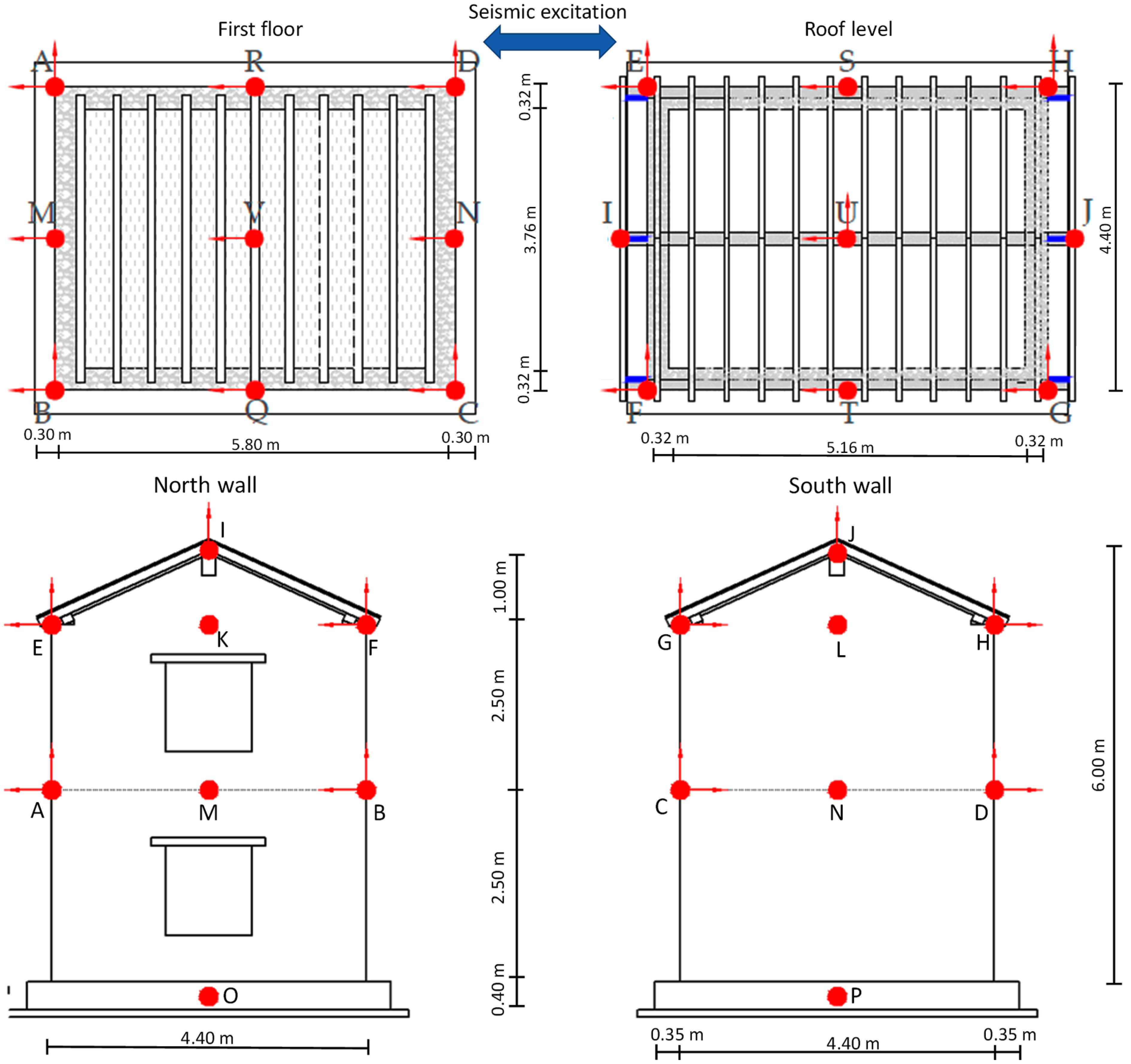
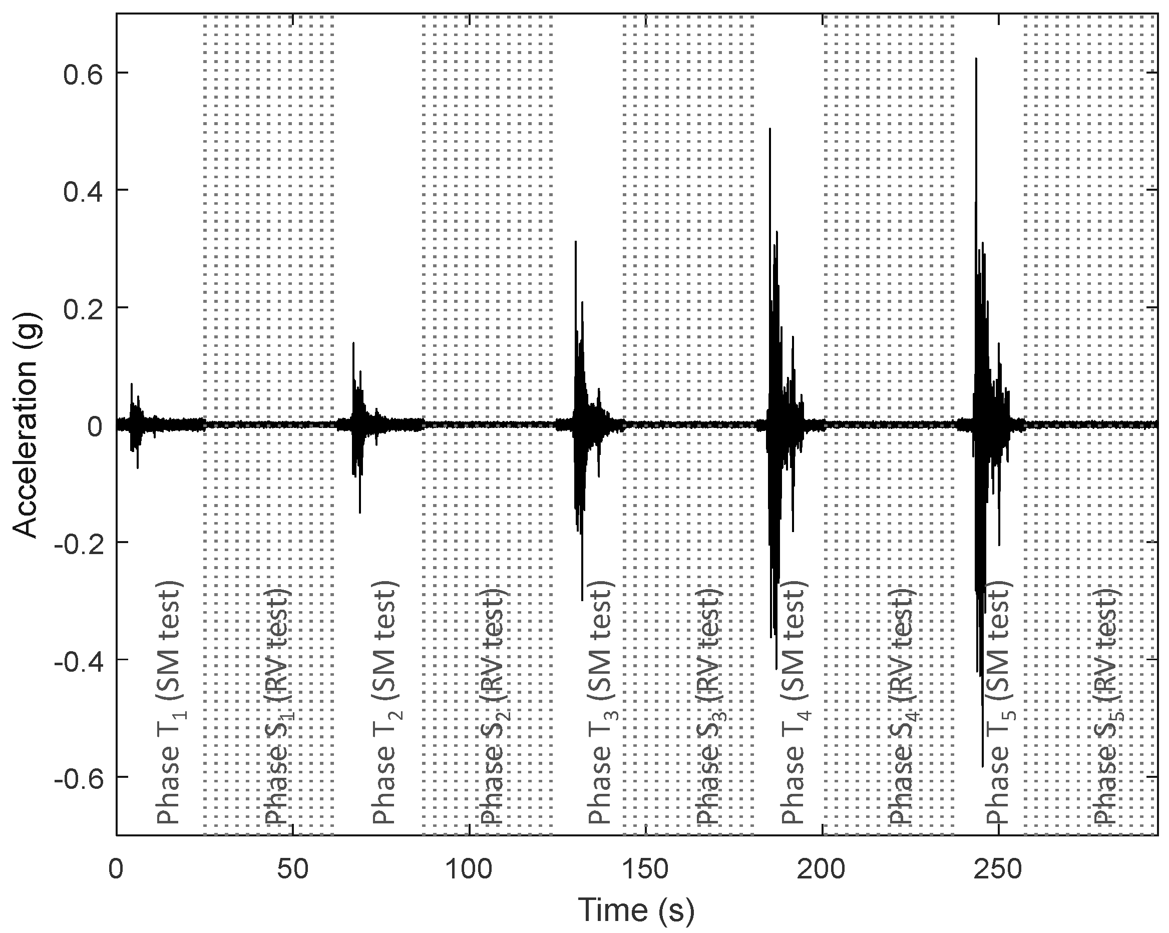
2. Brief Description of the Shaking Table Test Procedure and Response of the Building

A full-scale, two-storey unreinforced stone masonry (URSM) building, 5.80 × 4.40 m² in plan and 6 m high (Figure 1), with flexible diaphragms [20], was tested on a shaking table in Eucentre (Pavia, Italy) to investigate the nonlinear behaviour and the failure mechanism of the existing URSM structures. The details of the experiment can be found in [28].

A sequence of five test series for a progressively increasing seismic intensity was performed by scaling the natural accelerogram of the 1979 Montenegro earthquake along the longitudinal north–south (NS) direction of the URSM building (Figure 2).

The test structure during the fifth phase exhibited a local failure mechanism, characterised by a rocking non-linear (NL) response [29,30,31] of a part of the north second floor wall (perpendicular to the excitation).

Each dynamic test on the shaking table was preceded by calibration tests of random vibrations (stationary process) and preliminary modal identification was performed by recording the vibrations induced in the structure due to random noise.

Figure 2 presents the sequence of the test phases; after each strong motion T_i phase, there is a random stationary vibration S_i test. Detection and monitoring of the structural response in terms of accelerations in the current test series was performed using force feedback capacitive accelerometers. Their position was located on the critical zones of the structure, as presented in Figure 1.

The strong motion tests performed at low levels of PGA, namely T₁ to T₃, with a nominal PGA 0.05 g, 0.10 g and 0.20 g (and actual values ranging from 0.074 to 0.315 g as shown in Figure 2), did not induce visible damage to the structure. Only minor cracks were visible on west and east façades, which were parallel to the excitation (Figure 3). Dynamic identification showed, however, the existence of damage as early as the first phase [21].

The test T₅ performed at a nominal PGA of 0.40 g (and an actual one at 0.629 g, as shown in Figure 2) reached a close to the collapse state (Figure 4). The collapse mechanism had been already formed in the previous test phase T₄ at a nominal PGA of 0.30 g (actual PGA = 0.509 g), where the west wall presented stepped diagonal cracks at its top and bottom of the second-floor north pier, as shown with black lines in Figure 4. The collapse mechanism involved the upper part of the north façade (perpendicular to the excitation), which tended to overturn out-of-plane, the two spandrel beams and wooden lintels on the west and east walls (parallel to the seismic excitation), which rotated and slid on the lintel support, and the gable wall of the south façade, which also tended to overturn following the motion of the north wall due to their connection through the ridge beam (Figure 4).

The stationary tests preceded each strong motion tests and a final stationary test S₅ followed the strong motion test T₅. However, it should be noted that at this test, the structure was mildly reinforced with ties to prevent a total collapse of the facades.

3. State-Space Model of the Acceleration Measurements

The frequency characteristics of the URSM building subjected to subsequent oscillations with gradually increasing intensity vary substantially, as it experiences heavy damage over almost the entire NL domain up to collapse. ERA is able to decompose modes, even when they are very close and coupled. The first step of this method is to calculate the impulse response from the frequency response H(z) of the random vibration tests using the inverse Z-transform for the discrete system, which is as follows:

$$\left\{h\left(t\right)\right\}={\mathcal{Z}}^{-1}\left\{H\left(z\right)\right\}$$

(1)

where {h(t)}^T is the p × n impulse response vector at a given time step for the n sensors of the building.The key point of the method relies on obtaining the system Markov parameters directly from the impulse response {h(t)}, forming the Hankel matrix from the test data [32]. The realisation of the system matrices A, B and C is carried out by the singular value decomposition (SVD) [33] of the estimated Hankel and shifted Hankel matrices H(1) and H(2). The state matrices A, B and C are obtained as follows [34]:

$$\left[A\right]=\left[H(1\right){]}^{*}\left[H\right]\left[H(2\right){]}^{*}$$

(2a)

$$\left[B\right]=\left[H(2\right){]}_{,1}$$

(2b)

$$\left[C\right]=\left[H(1\right)]{\left[D\right]}_{1:m,}$$

(2c)

The physical representation of the system Σ{A, B, C, D} is obtained using a similarity transformation [35], since the direct interpretation of the state-space matrices is only possible in limited cases e.g., [32]. The SVD of the discrete state matrix A is applied as follows [32,36]:

$$\left[A\right]=\left[\Psi \right]\left[\Lambda \right]{[\Psi ]}^{-1}$$

(3)

In the latter Equation (3) Λ is a uniquely determined diagonal matrix containing the complex singular values {λ_k} of A that represent the eigenvalues of the system and Ψ is a square matrix. The eigenvectors Φ ={φ_i} of the system are obtained as follows:

$$\left[\Phi \right]=\left[C\right]\left[\Psi \right]$$

(4)

It should be emphasized that the eigen values λ_k of the discrete system should be transformed to the continuous-time model. λ_i denotes the Eigen values of the continuous-time system, A_c the continuous-time state matrix, F_s the frequency sampling and ζ_i the modal damping. Then, it can be easily found that [14,37]

$$\underset{¯}{A}=e^{\frac{1}{F_s}{\underset{¯}{A}}_c}$$

(5a)

$${\lambda }_i=F_s\left(\mathit{ln}{\lambda }_k\right)$$

(5b)

$${\zeta }_i=\frac{\mathit{Re}\left({\lambda }_i\right)}{\left|{\lambda }_i\right|}$$

(5c)

It is noted here that the transformation of Equation (5) is not unique as any ±κ·2π, κЄℤ can be added to the natural logarithm [14].

4. FEM Calibration

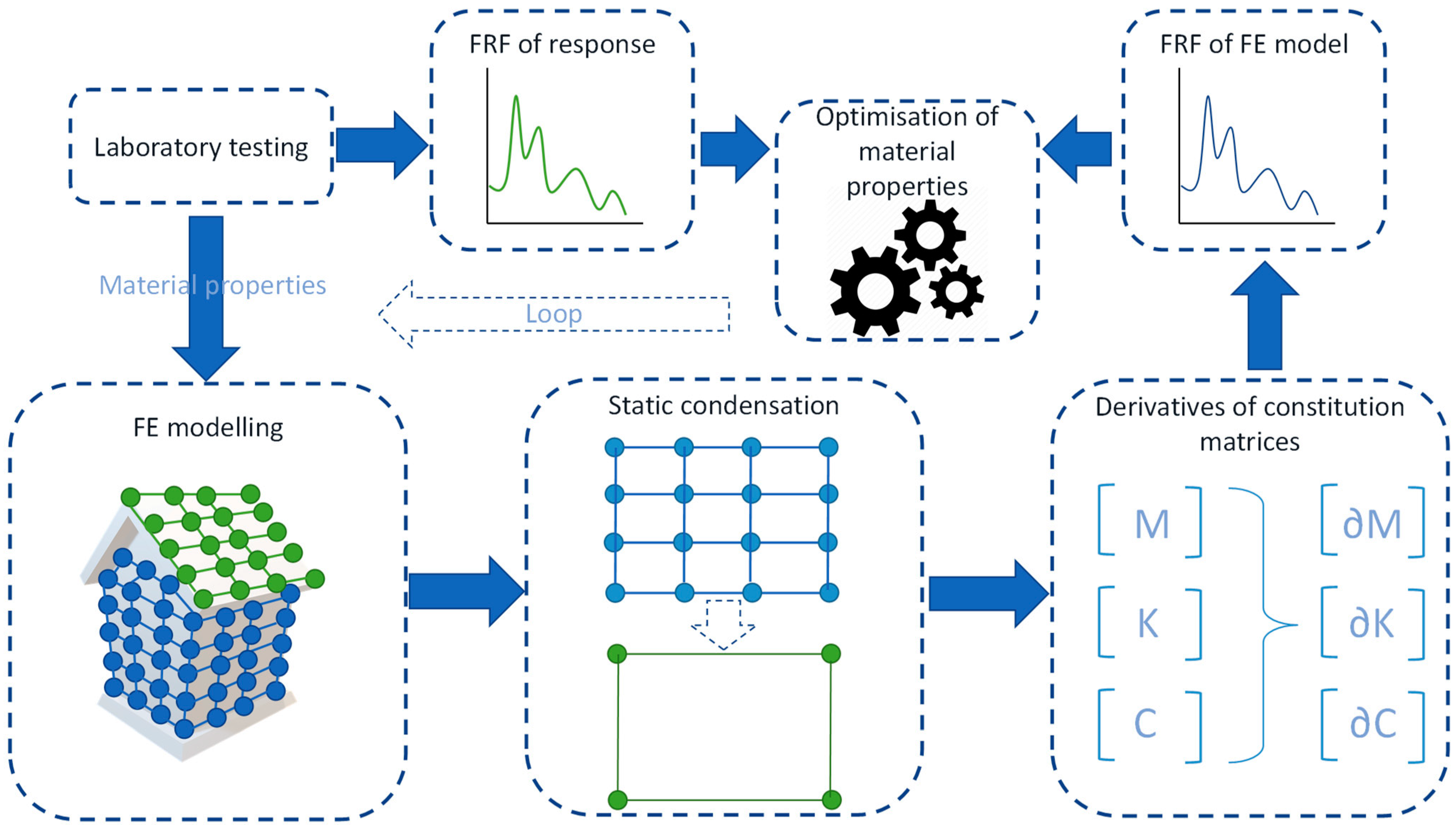
4.1. Overview of the Calibration Procedure

By analysing the random vibration tests, it is possible to estimate the equivalent elastic properties of the building after the suffered damage (Figure 3 and Figure 4), due to the preceding strong motion tests (sequence of tests presented in Figure 2). The main assumption of the procedure is that each structural wall (east, west, north and south) and the flexible diaphragms can have different elastic moduli due to cracking.

The procedure is illustrated in Figure 5 and can be summarised as follows:

• Step 1: from the laboratory testing, the material properties and the frequency response functions (FRF’s) of the structure are obtained.
• Step 2: an FE model of the structure is built based on the previously found material properties.
• Step 3: static condensation is performed to reduce the degrees of freedom (DOFs) of the model.
• Step 4: the derivatives of the constitution matrices of the model (M mass, K stiffness and C damping) are estimated.
• Step 5: using the data from steps 2 to 4, the FRF’s are estimated.
• Step 6: FRF’s from steps 1 and 6 are compared and new material properties are estimated.
• Step 7: the optimisation procedure returns to step 2 until the comparison shows an acceptable convergence.

Steps 2 to 7 are explicitly described in the following Section 4.2 to Section 4.7. As aforementioned, the basic assumption of the FE modelling is to assume that masonry remains a continuum and cracking is not directly simulated but indirectly taken into account by the modified mechanical properties of an equivalent elastic response, in accordance with the smeared crack approach. The initial values for the calibration procedure are those found from the material testing.

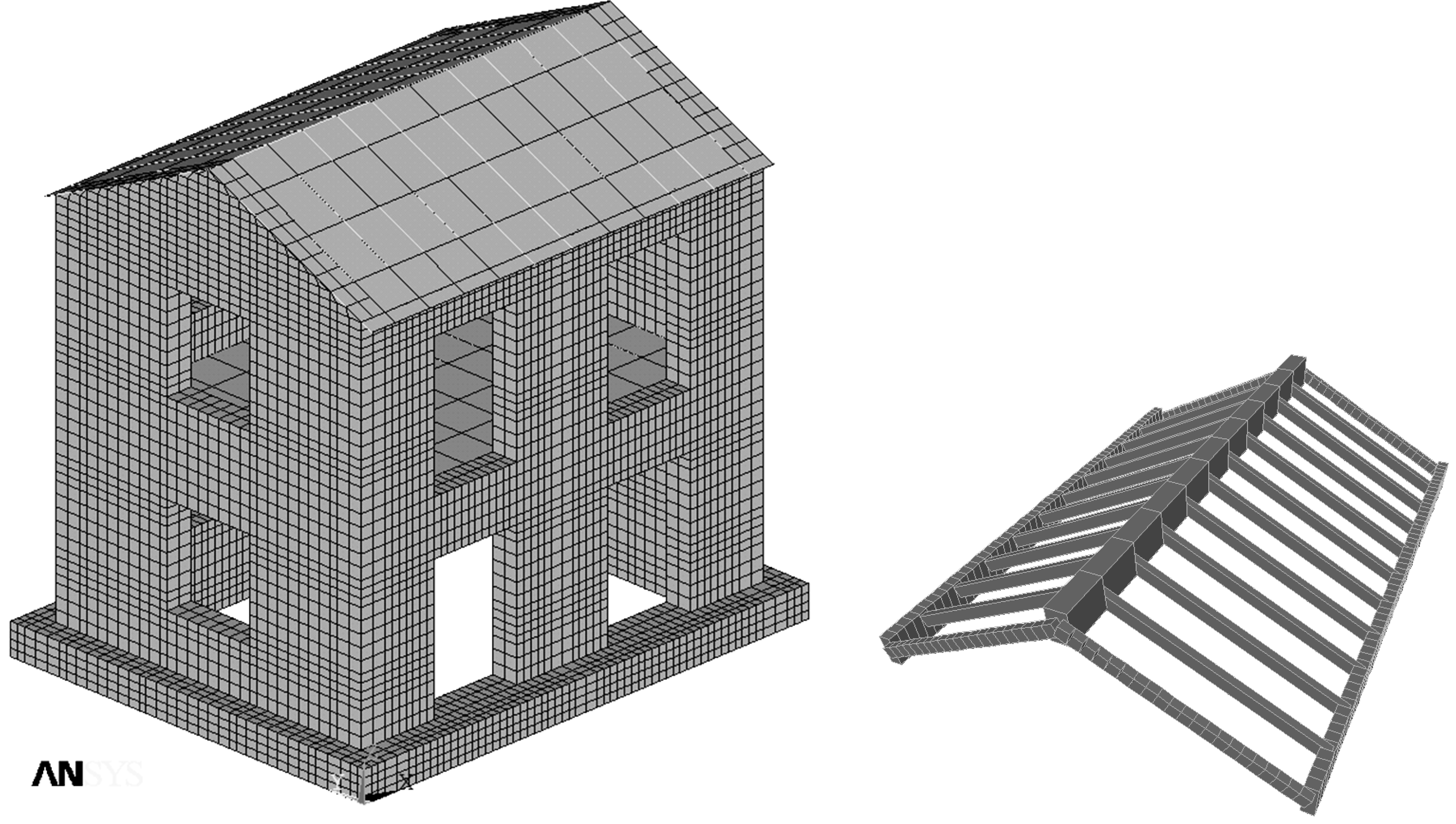
4.2. Set-Up of the FE Model and Calibration Parameters

A linear elastic FE model is employed following the exact dimensions of the structure to study the evolution of the material properties due to cracking and damage. The model is elastic, as it is calibrated with the elastic response of the stationary random vibrations. The building suffers damage that accumulates in every next test phase [38]. Therefore, the elastic properties identified from the random vibration tests in each test phase i reflect the secant modulus of masonry walls, assuming a smeared crack equivalent elastic modulus of the damaged structure up to the specific test phase i. This approach simulates the propagation of cracks inside the body of masonry by modifying its elastic properties, i.e., using ‘softer’ ones for a cracked wall.

Masonry as a material is far from an elastic homogeneous media, with uniform and constant properties throughout. On the contrary, masonry is a material characterised by strong heterogeneity on a micro or meso-scale. Consequently, the macroscopic properties depend strongly on the configuration of the construction. Brickwork has a standard pattern that is repeatedly replicated [39]. Stonework, on the contrary, has an intrinsic ‘non-periodic’ construction, resulting from the variability in the stone units and mortar joints. Moreover, the construction of the walls in a double-wythe fashion, scarcely connected between them at the edges, makes the equivalent homogenous isotropic elastic properties more problematic. Therefore, an anisotropic model fits better with the actual situation.

During the calibration process, masonry is considered as an orthotropic material [40,41,42,43,44]. Orthotropy is essential to study the evolution of the shear to elastic moduli ratio G/E. Masonry properties vary among the walls in the calibration process as a result of the different cracking and despite the fact that all of them were built from the same constituents and with the same technique.

The shear moduli G_i is assumed equal to all the three directions, as this was estimated from diagonal compression tests and no testing was performed for the out-of-plane one. Elastic moduli of masonry in the out-of-plane direction E₂ and the horizontal one E₃, as no testing was performed, are assumed proportional to the 80% of the vertical direction E₁ based on standard values from the literature [39,41,42,45]. The calibration parameters are presented in

Table 1. The material parameters considered in the calibration process.

	E1	E2	E3	G1	G2	G3
West wall	P1	0.8P1	0.8P1	P2	P2	P2
East wall	P3	0.8P3	0.8P3	P4	P4	P4
North wall	P5	0.8P5	0.8P5	0.33P5	0.33P5	0.33P5
South wall	P5	0.8P5	0.8P5	0.33P5	0.33P5	0.33P5
Diaphragm	-	-	-	P6	P6	P6

. The north and south walls presented a similar damage mechanism involving the gable roof, and therefore have the same parameters P₅. As the damage of the north and south walls is out-of-plane, the shear modulus is assumed to remain constant (i.e., G/E = 0.33).

The initial material properties are determined from material testing [46]. Then, the calibration of the FE model is carried out using the FEMCali software [9]. The FE model is built in ANSYS [47] (Figure 6) using the following elements:

• Eight-node solid elements (SOLID185) with three translational DOFs in each node to simulate the concrete base of the structure and the masonry walls. Shell elements with rotational DOFs could be used alternatively but they can simulate the connections with timber less accurately.
• Four-node shell elements (SHELL63) with two in-plane translational DOFs in each node to simulate the timber floor diaphragm and the timber roof diaphragm.
• Two-node beam elements (BEAM4) with six DOFs (translational and rotational) in each node to simulate the timber beams of the floor and the roof.

It is noted that the floor’s diaphragm nodes are not connected to the north and south walls but only to the west and east walls, parallel to the vibration direction. A meticulous simulation of this connection could include NL compression-only springs to simulate the interaction with these walls. However, for the stationary tests, this is deemed unnecessary.

The nominal thickness of the walls is 32 cm (Figure 1). Solid elements (SOLID185) with three DOFs in each node are used to simulate both in-plane (membrane action) and out-of-plane (bending) actions. The roof of the building is covered with 430 tiles, each one weighing 3 kg, i.e., 3 × 9.81 = 29.43 N; hence, the total weight of the tiles can be estimated as 12.7 kN. The corresponding mass is distributed evenly in the 90 joints that comprise the roof structure. Each of the 81 nodes of the first-floor diaphragm has an added mass equal to 0.39 t; hence, the total mass of 30.6 t has been evenly distributed. These added masses have only in-plane DOFs to avoid any unwanted vibration in the vertical axis.

Then, an analysis is performed to retrieve the mass M and stiffness K matrices. The damping matrix C_ζ is constructed at a later phase numerically using the estimated damping from Equation (5c) of the experimental modal identification. In the follοwing expression, Φ is the modal matrix and Z is a diagonal matrix that contains the modal damping ratios ζ_i identified through the modal identification procedure.

$$\left[C_{\zeta }\right]=\left(\left[M\right]\left[\Phi \right]{[M]}^{-1}\right)Z\left({[M]}^{-1}\left[\Phi \right]\left[M\right]\right)$$

(6)

The initial elastic properties of the “intact” walls are determined from a set of six vertical compression tests, six diagonal compression tests and five in-plane cyclic shear tests [48]. From uniaxial compression tests, stress–strain curves were obtained, together with an estimation of the compressive strength of the masonry. The conventional shear modulus was calculated similarly from the shear stress–strain curves obtained in the diagonal compression tests, as a secant modulus at 1/3 of the panel strength. The shear modulus of the diaphragm G_diaph is 354 MPa, whose equivalent thickness is 4 cm. The main results are summarized in

Table 2. Mechanical properties (compressive strength f_m, elastic modulus E, tensile strength f_t and shear modulus) of stone masonry in MPa.

	fm	E	ft	G
Mean	3.28	2550	0.137	840
St. Dev.	0.26	345	0.031	125
c.o.v.	8%	13.50%	21.80%	14.80%

. The initial ratio of shear to elastic moduli G/E is 0.33 smaller than the suggested value in many codes 0.4 [49]. The fact that the proposed ratio of G/E in codes is larger than the actual one has been reported in several studies (e.g., [40,42,43,44]). The experimentally found ratio 0.33 would correspond to the marginal value for a Poisson ratio v = 0.5 of a homogeneous material. This value drops as cracking appears, as shown in the next sections; therefore, the assumption of a heterogeneous material is the only valid one for the current analysis.

4.3. Static Condensation of the FE Model

A key issue associated with full scale experiments of structures is the location of sensors. Due to availability, computation capabilities and cost considerations, a minimum number of sensors should be placed so that the locations fulfill the requirements of an efficient system identification. However, the FE model of the structure includes thousands of DOFs, with some eigenvalues outside the frequency range of practical interest. For this reason, it is necessary to reduce the order of the FE model to the size of measurements accordingly, in order to transform the high dimensional system of equations from the FE modeling of the mechanical structure into the lower experimental dimensionality.

The static condensation is the basis for the model reduction [50]. An FE model of the structure under investigation is prepared using the mechanical properties from monotonic and cyclic tests of the materials before the shaking table test (Figure 6). This model is constrained by applying the relevant laboratory conditions and restrains and properly loaded with gravitational loads. The total number of the degrees of freedom (DOFs) is denoted as σ, normally equal to the double, threefold or sixfold of the number of nodes of shells, solids and beams, respectively. This set σ can be subdivided into c (constrained) and f (free) DOFs. Static analysis equations (i.e., forces F_f equal to the product of stiffness K_ff times the displacements δ_f of the f DOFs) take on a matrix form after applying the respective constraint conditions, which are as follows:

$$\left[K_{ff}\right]\cdot \left\{{\delta }_f\right\}=\left\{F_f\right\}$$

(7)

Free (f) DOFs are divided in two sets, m (masters) and s (slaves) DOFs. Master DOFs are kept during the reduction process, while slave DOFs are those who should be eliminated. Therefore, Equation (7) is decomposed in m and s DOFs as follows:

$$\left[\begin{array}{cc}{K}_{mm}& K_{ms}\\ K_{sm}& K_{ss}\end{array}\right]\cdot \left\{\begin{array}{c}{\delta }_m\\ {\delta }_s\end{array}\right\}=\left\{\begin{array}{c}{F}_m\\ F_s\end{array}\right\}$$

(8)

4.4. Estimation of the Derivatives of the FE Matrices

The direct optimisation of the deviation function between the FE model and the experimental data using, in each step, a new FE analysis should be avoided due to the high computational cost involved in the procedure. This would lead inevitably to an almost infinite time for the FE matrices that have an order of magnitude of ten thousand approximately. In order to perform an efficient iterative update of the FE model, it is necessary to estimate the derivatives of the mass, damping and stiffness matrices M, C, K $\in {ℝ}^{n\times n}$. This method avoids the computational challenges of building the structural matrices using a direct FE analysis by using an extrapolation method to obtain a reliable difference quotient for the structural matrices [9]. The Newton central difference-quotient is used in Equation (9). The gradient of the structural matrices, with respect to the parameters to be calibrated, is obtained using the step-wise Ridders interpolation procedure to minimise the error [51].

$$f^{\prime }\left(x\right)\approx \underset{h\to 0}{lim}\frac{f\left(x+h\right)-f\left(x-h\right)}{2h}$$

(9)

4.5. Estimation of the Frequency Response Function of the FE Model

The state-space formulation of the building specimen is based on the transformation of the second order differential system equation into the form of a first order matrix differential equation, which can be easily solved using numerical integration. Thus, the system is represented by a model that can be used to retrieve the dynamic response of any general input excitation. It is emphasized that the state-space formulation a priori assumes that the system performs linearly; therefore, the matrix model remains constant during the response [52]. As aforementioned, the shaking table tests of the two-storey masonry building presents a highly NL response, as extensive cracking appears at high intensities. However, by focusing only on random vibration tests, which are performed at a low magnitude, the response is linear, and it is possible to measure the ‘linear effective’ response of the gradually damaged building specimen that represents the secant moduli after the damage of each strong motion test phase.

The response of an n degrees-of-freedom (DOFs) system excited by random vibration tests is governed by a second order differential equation. The differential equation of a continuous-time system is solved for the highest order derivative in Equation (10), where M, C, K $\in {ℝ}^{n\times n}$ stand for the building structural matrices of mass, damping and stiffness, respectively. The input matrix is denoted as B $\in {ℝ}^{n\times p}$ and $u\left(t\right)\in {ℝ}^p$ represents the input signals sent to the system, where p is equal to 1. Equation (10) is a large scale second order differential-algebraic equation, assuming that M is invertible, which is the case for real structures.

$$\ddot{y}\left(t\right)=-M^{-1}{C}_{\zeta }\dot{y}\left(t\right)-M^{-1}Ky\left(t\right)+M^{-1}{B}_{0}u\left(t\right)$$

(10)

Using the following transform,

$$x\left(t\right)=\dot{y}\left(t\right)+y\left(t\right).$$

(11)

Equation (10) takes the following expression:

$$\frac{dx}{dt}=\underset{¯}{A}x+\underset{¯}{B}u,\mathrm{where}A=\left[\begin{array}{cc}{0}_{n\times n}& I_{n\times n}\\ -M^{-1}K& -M^{-1}{C}_{\zeta }\end{array}\right],\mathrm{and}B=\left[\begin{array}{c}{0}_{n\times 1}\\ M^{-1}{B}_0\end{array}\right]$$

(12)

Equation (12) describe the dynamics of the vibration of the two-storey URSM structure in terms of the state variable $x\left(t\right)\in {ℝ}^n$ in Equation (11). Then, the following expressions relate the measured output $y\left(t\right)\in {ℝ}^m$ to the state variable:

$$y\left(t\right)=C\cdot x\left(t\right)+D\cdot u\left(t\right),C=\left[\begin{array}{cc}-C_a{M}^{-1}K& -C_{\zeta }{M}^{-1}K\end{array}\right],D=\left[-C_a{M}^{-1}B\right]$$

(13)

For a discrete state space system, the transfer function matrix can be obtained, applying the z-transform of Equation (11) as follows [37]:

$$H\left(z\right)=C {\left(z I - A\right)}^{-1} B+D$$

(14)

4.6. Estimation of Deviation between FE Model and Recording Response

The deviation ε between the experimental data and the FE model is estimated using the frequency response function H(jω). The error e(jω) is defined as the ratio of frequency response functions between the FE model H_FE(jω) and the test data H_test(jω) [8] and can be obtained as follows:

$$e\left(j{\omega }_i\right)=\mathit{ln}\frac{H_{FE}\left(j{\omega }_i\right)}{H_{test}\left(j{\omega }_i\right)}$$

(15)

Then, the deviation is the vector of the real and imaginary parts of the error is defined as follows [8]:

$$\overrightarrow{{\epsilon }_i}=\frac{\left\{\begin{array}{cc}\mathit{Re}(e_i)& Im(e_i)\end{array}\right\}}{\sqrt{2\mathit{max}\left(i\right)}}$$

(16)

4.7. Iterative Method for Solving the Calibration Set of Equations

The minimum of the function of the deviation ε(p_i), i = {1,6} between the recordings and the response of the FEM model for the selected parameters p_i is identified using the steepest descent method. The Levenberg–Marquardt algorithm [53] for fitting a nonlinear regression in order to solve the non-linear least squares problem has been applied. The algorithm interpolates between the Gauss–Newton algorithm and the method of gradient descent. To find the model parameters, the initial estimates are updated during each iteration in the downhill direction to the gradient, decreasing the average square error with a damped least-squares approach. However, a standard local search approach is only applicable for the non-linear least-squares optimization, leading to a good approximation, as long as the estimates are close to the real values. The Jacobian matrix is built from the partial derivatives that are computed numerically during each iteration. The calibrated values of each test phase are used as the starting points for the optimisation loop of the next test phase.

5. Calibrated Model

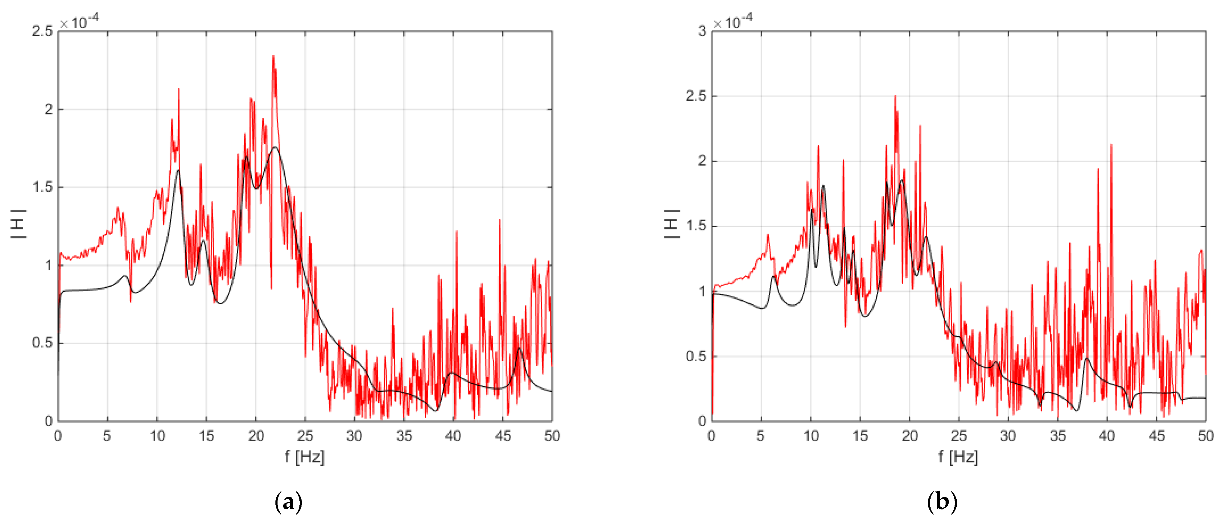
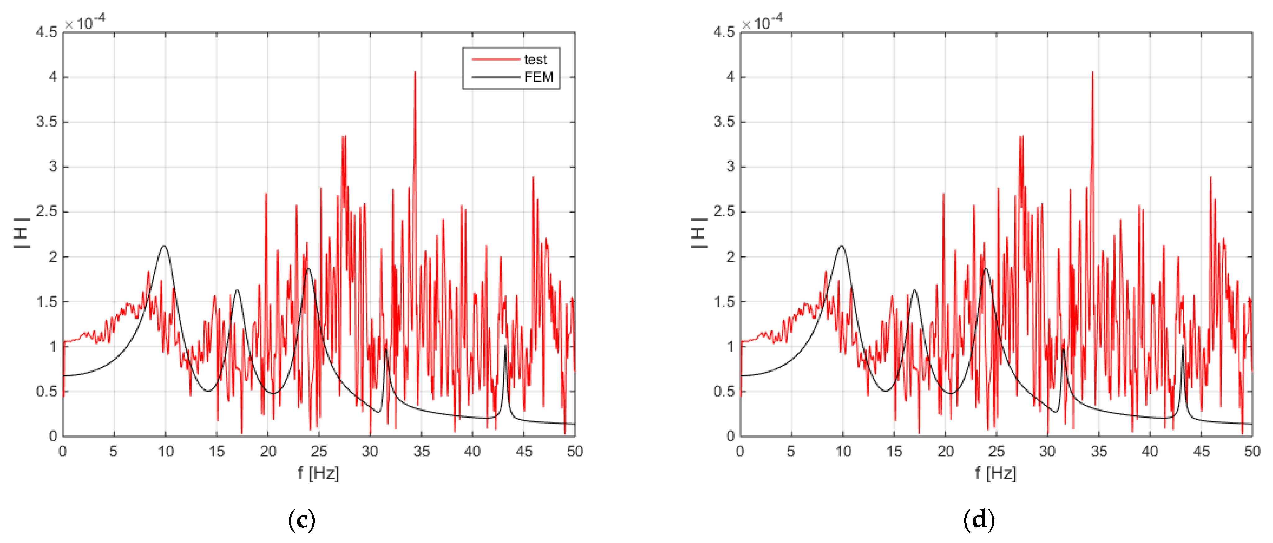
5.1. Calibrated Frequency Response

The metric used to optimise the difference between the experimental data and the FE model is the frequency response visualised in Figure 7. It is shown that the calibration process achieves very good results. Moreover, it is observed that the deviation of the calibration increases with the magnitude of the shaking. This is an inherent weakness of the FE model and the procedure. The adopted smeared crack model does not discriminate among the floor levels and piers, which would result in higher ‘heterogeneity’ between structural members as a result of the different level of damage and more accurate depiction of the cracking. However, as already mentioned, a higher number of variables in the calibration model leads to a higher numerical cost. Therefore, a discrepancy in the FR is justified with the test phases of the experiment.

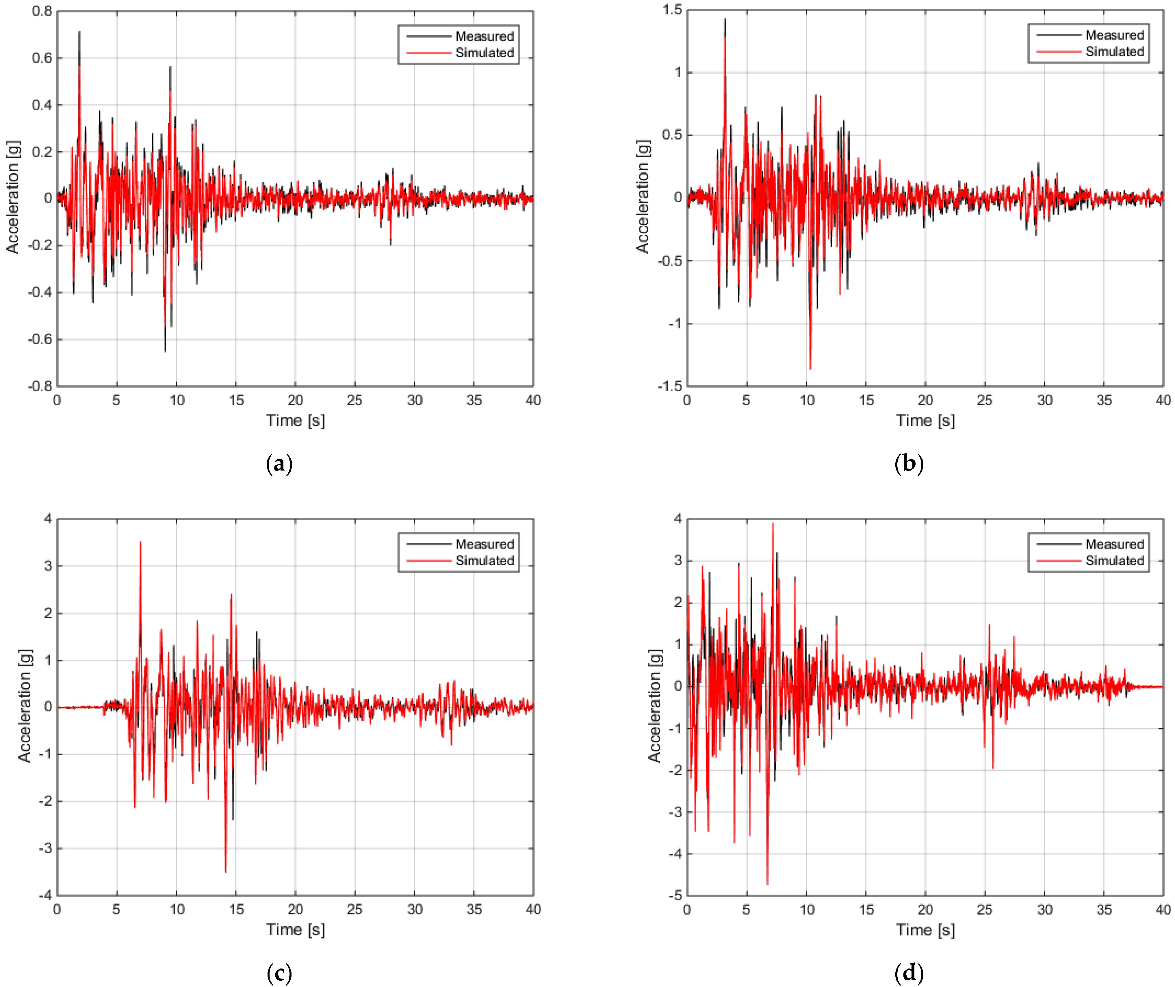
5.2. Calibrated Acceleration Response

The calibrated FE models are loaded with the strong motion time history (Figure 2) and the response in point B (Figure 1) of the structure is detected for each test phase depicted in Figure 8. Therefore, the identified mechanical properties are assumed that they represent the effective (secant) elastic properties of the NL structure.

It can be observed in Figure 8 that the FE model response is very accurate with regard to the frequency content and peaks when compared to the experimental results for the first two test phases and there is a slight difference in the estimation of the last two test phases. Therefore, the effective calibrated properties can be assumed to be representative of the structural behaviour given the simplifications of the smeared crack approach. In any case, the efficiency is better for the lower magnitude tests.

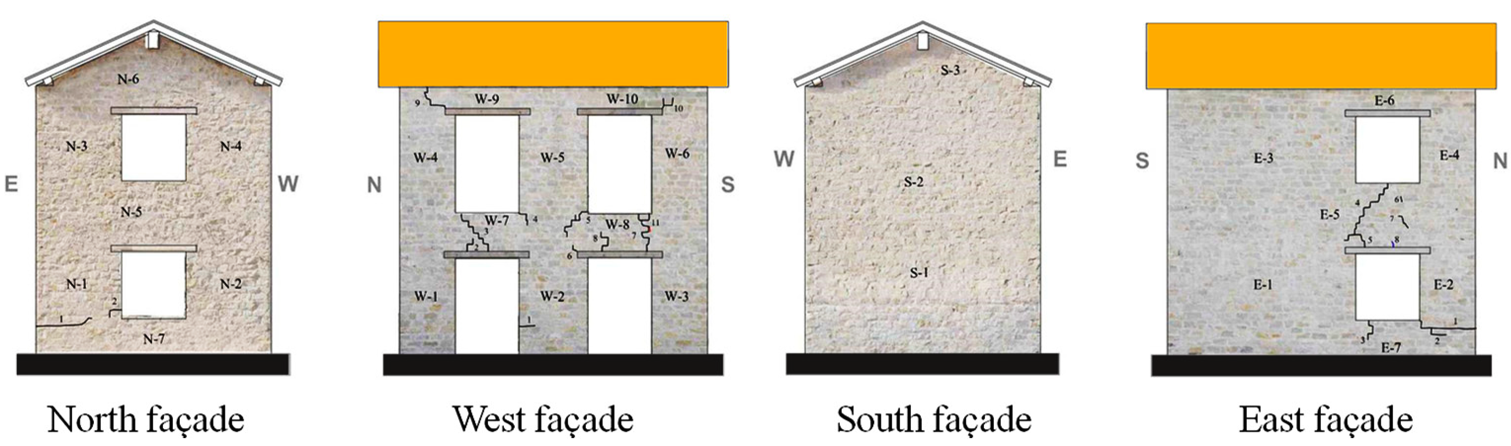
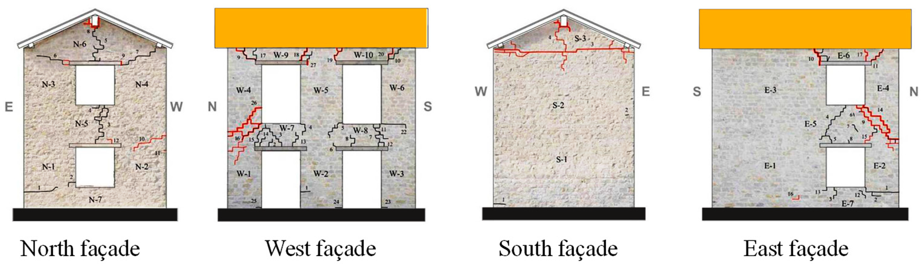
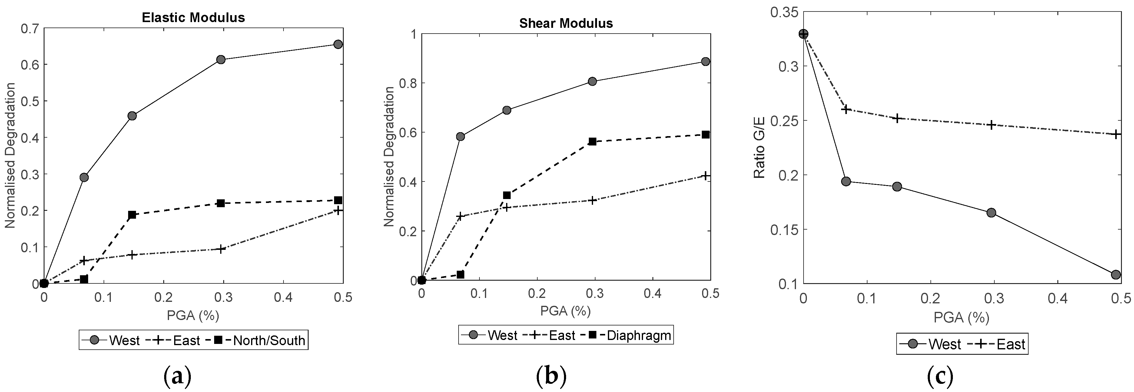
5.3. Mechanical Deterioration

The normalised degradation p_i,χ of the parameter P_i,χ(Table 1) is defined as follows, where P_i,χ is the value of the parameter i at the step of the analysis χ:

$$P_{i,\chi }=P_{i,\chi -1}\left(1-p_{i,\chi }\right)$$

(17)

Table 3. Elastic (E) and shear (G) moduli in GPa for each test phase of the building’s structural members.

Member	Modulus	Initial	Phase 1	Phase 2	Phase 3	Phase 4
East wall	E	2.55	1.81	1.38	0.99	0.88
	G	0.84	0.35	0.26	0.16	0.10
West wall	E	2.55	2.39	2.35	2.31	2.04
	G	0.84	0.62	0.59	0.57	0.48
OOP walls	E	2.55	2.52	2.07	1.99	1.97
Diaphragm	G	0.35	0.35	0.23	0.16	0.14

and Figure 9 present the evolution from phase to phase of the equivalent elastic moduli and the normalised degradation p_i,χ for each parameter. The degradation of the elastic modulus E₁ of the west wall (parallel to the excitation) presents a regular shape (Figure 9a), due to the fact that the wall has a rather uniform distribution of cracks in all of its piers and spandrels (see Figure 3 and Figure 4). On the contrary, the degradation of the east wall (parallel to the excitation) is lower and has a sudden increase from the third to the fourth phase (Figure 9a). This is in line with the diagonal cracks that appear in this wall at this phase (see Figure 3 and Figure 4). The elastic modulus of the north and south facades (perpendicular to the excitation) has a steeper increase in the degradation between the second to the third phases when the horizontal cracks are initially formed and subsequently propagated (Figure 9a). Therefore, the analysis shows very good coincidence with the actual damage of the structure.

The degradation of shear moduli appears to be higher than that of the elastic moduli. In the last phase, the degradation approaches 60 and 90% for the east and west walls, respectively (Figure 9b). East wall has again a very steep escalation of the degradation after the second phase, which keeps increasing in the next two phases (Figure 9b). The evolution of the degradation of the diaphragm shear modulus has a smoother change, which shows an important increase (i.e., a decrease in the actual value of the shear modulus) in the third and the fourth phases (Figure 9b), during which the damage mechanism is formed. The drop of the shear modulus in the diaphragm occurs due to the shearing of the wood around the area of the stitching screws and nails of the wooden floor planks. During the first and the last phase, only a small change in the shear modulus is observed.

The ratios of shear to elastic moduli for the east and west walls increase with the magnitude of the vibration. The initial value G/E = 0.33 drops below 30%, even from the first phase of the vibration (Figure 9c). East wall appears to have a ratio value that approaches 0.25, whereas west wall’s G/E ratio keeps decreasing more approaching 10% (Figure 9c). These low values have also been noticed experimentally [40,44].

6. Conclusions

FE calibration with the results derived from SSI and state-space modelling was carried out for the evaluation of the material secant moduli of a URSM building consecutively tested on a shaking table. The building was full-scale and experienced increasing levels of damage as the vibration intensity augmented. Random vibration tests after the strong motion tests allowed to derive a state-space model of the structure and calibrate a FE simulation of the building. The calibration suggests a gradual deterioration of the mechanical parameters that comprised the materials of the structure. Six parameters were chosen to be calibrated in the framework of a smeared cracked approach, involving the elastic moduli of the walls and the wooden diaphragm of the building. The selection of these parameters is a balance between the need to differentiate the mechanical properties of the structural parts with variable responses and damage and on the other hand, to maintain a reasonable numerical cost of the procedure.

The calibration procedure adopts a deviation metric based on the frequency response between the experimental data and the FE response. The optimisation process which follows minimises the deviation and estimates the best-fit parameters. The gradients of the structural matrices are numerically defined using Ridders interpolation. The calibration shows robust and reliable results as compared to the structural response and damage.

The results of the analyses give an insight into the structural response of URSM buildings and show a degradation of the mechanical characteristics with increasing shaking intensity in the framework of an equivalent linear elastic model. Under strong shaking, the structure presents a significant degradation of the stiffness of its structural members, in accordance with the actual damage of the building. The shear modulus appears to decrease more than the elastic modulus of the respective walls. The west wall which is uniformly damaged has a regular curve with increasing shaking intensity. The east wall instead has steep drops in some phases. The shear modulus of the timber diaphragm deteriorates from phase to phase. The shear to elastic moduli ratio drops to values as low as 10% for the more damaged wall.

References

1. Aras, F.; Krstevska, L.; Altay, G.; Tashkov, L. Experimental and numerical modal analyses of a historical masonry palace. Constr. Build. Mater. 2011, 25, 81–91. [Google Scholar] [CrossRef]
2. Krstevska, L.; Tashkov, L.; Gocevski, V.; Garevski, M. Experimental and analytical investigation of seismic stability of masonry walls at Beauharnois powerhouse. Bull. Earthq. Eng. 2009, 8, 421–450. [Google Scholar] [CrossRef]
3. Kerschen, G.; Worden, K.; Vakakis, A.F.; Golinval, J.-C. Past, present and future of nonlinear system identification in structural dynamics. Mech. Syst. Signal Process. 2006, 20, 505–592. [Google Scholar] [CrossRef]
4. Doebling, S.W. Structural dynamics model validation: Pushing the envelope. In Proceedings of the International Conference on Structural Dynamics Modelling: Test, Analysis, Correlation and Validation, Madeira, Portugal, 3–5 June 2002. [Google Scholar]
5. Allemang, R.J.; Brown, D.L. A correlation coefficient for modal vector analysis. In Proceedings of the First International Modal Analysis Conference; Union Coll: Orlando, FL, USA, 1982; pp. 110–116. [Google Scholar]
6. Lourenço, P.B.; Trujillo, A.; Mendes, N.; Ramos, L.F. Seismic performance of the St. George of the Latins church: Lessons learned from studying masonry ruins. Eng. Struct. 2012, 40, 501–518. [Google Scholar] [CrossRef]
7. Aguilar, R.; Marques, R.; Sovero, K.; Martel, C.; Trujillano, F.; Boroschek, R. Investigations on the structural behaviour of archaeological heritage in Peru: From survey to seismic assessment. Eng. Struct. 2015, 95, 94–111. [Google Scholar] [CrossRef]
8. Abrahamsson, T.S.; Kammer, D. FEM Calibration with FRF Damping Equalization. In Model Validation and Uncertainty Quantification; Atamturktur, H.S., Moaveni, B., Papadimitriou, C., Schoenherr, T., Eds.; Conference Proceedings of the Society for Experimental Mechanics Series; Springer: Cham, Switzerland, 2014; Volume 3, pp. 265–278. ISBN 978-3-319-04551-1. [Google Scholar]
9. Abrahamsson, T.J.S.; Kammer, D.C. Finite element model calibration using frequency responses with damping equalization. Mech. Syst. Signal Process. 2015, 62–63, 218–234. [Google Scholar] [CrossRef]
10. Van Overschee, P.; De Moor, B. N4SID: Subspace algorithms for the identification of combined deterministic-stochastic systems. Automatica 1994, 30, 75–93. [Google Scholar] [CrossRef]
11. Ljung, L.; McKelvey, T. Subspace identification from closed loop data. Signal Process. 1996, 52, 209–215. [Google Scholar] [CrossRef]
12. Peeters, B.; De Roeck, G. Reference-Based Stochastic Subspace Identification for Output-Only Modal Analysis. Mech. Syst. Signal Process. 1999, 13, 855–878. [Google Scholar] [CrossRef]
13. Deraemaeker, A.; Reynders, E.; De Roeck, G.; Kullaa, J. Vibration-based structural health monitoring using output-only measurements under changing environment. Mech. Syst. Signal Process. 2008, 22, 34–56. [Google Scholar] [CrossRef]
14. Juang, J.-N.; Phan, M.Q.; Dewell, L. Identification and Control of Mechanical Systems; Cambridge University Press: Cambridge, UK, 2004; Volume 55, ISBN 0-521-78355-0. [Google Scholar]
15. Hoshiya, M.; Saito, E. Structural Identification by Extended Kalman Filter. J. Eng. Mech. 1984, 110, 1757–1770. [Google Scholar] [CrossRef]
16. Juang, J.-N.; Pappa, R.S. An eigensystem realization algorithm for modal parameter identification and model reduction. J. Guid. Control. Dyn. 1985, 8, 620–627. [Google Scholar] [CrossRef]
17. Hu, S.-L.J.; Yang, W.-L.; Liu, F.-S.; Li, H.-J. Fundamental comparison of time-domain experimental modal analysis methods based on high- and first-order matrix models. J. Sound Vib. 2014, 333, 6869–6884. [Google Scholar] [CrossRef]
18. Indirli, M.; Kouris, L.A.S.; Formisano, A.; Borg, R.P.; Mazzolani, F.M. Seismic Damage Assessment of Unreinforced Masonry Structures After The Abruzzo 2009 Earthquake: The Case Study of the Historical Centers of L’Aquila and Castelvecchio Subequo. Int. J. Archit. Herit. 2013, 7, 536–578. [Google Scholar] [CrossRef]
19. Kouris, L.A.S.; Borg, R.P.; Indirli, M. The L’Aquila Earthquake, April 6th, 2009: A review of seismic damage mechanisms. In Proceedings of the COST ACTION C26 “Urban Habitat Constructions under Catastrophic Events”, Final Conference, Naples, Italy, 16–19 September 2010; Mazzolani, F.M., Ed.; Taylor & Francis Group: London, UK, 2010; pp. 673–681. [Google Scholar]
20. Magenes, G.; Penna, A.; Galasco, A. A full-scale shaking table test on a two-storey stone masonry building. In Proceedings of the 14th European Conference on Earthquake Engineering, Ohrid, Republic of Macedonia, 30 August–3 September 2010. [Google Scholar]
21. Kouris, L.A.S.; Penna, A.; Magenes, G. Seismic damage diagnosis of a masonry building using short-term damping measurements. J. Sound Vib. 2017, 394, 366–391. [Google Scholar] [CrossRef]
22. Kouris, L.A.S. Dynamic Identification and Assessment of the Response of a Full Scale Unreinforced Masonry Building Tested on Shaking Table. Ph.D. Thesis, Istituto Universitario di Studi Superiori di Pavia, Pavia, Italy, 2015. [Google Scholar]
23. Kouris, L.A.S.; Penna, A.; Magenes, G. Dynamic Modification and Damage Propagation of a Two-Storey Full-Scale Masonry Building. Adv. Civ. Eng. 2019, 2019, 2396452. [Google Scholar] [CrossRef]
24. Aloisio, A.; Antonacci, E.; Fragiacomo, M.; Alaggio, R. The Recorded Seismic Response of the Santa Maria Di Collemaggio Basilica to Low-intensity Earthquakes. Int. J. Archit. Herit. 2021, 15, 229–247. [Google Scholar] [CrossRef]
25. Lorenzoni, F.; Casarin, F.; Caldon, M.; Islami, K.; Modena, C. Uncertainty quantification in structural health monitoring: Applications on cultural heritage buildings. Mech. Syst. Signal Process. 2016, 66–67, 268–281. [Google Scholar] [CrossRef]
26. Kouris, L.A.S.L.; Penna, A.; Magenes, G. Damage detection of an unreinforced stone masonry two storeys building based on damping estimate. In Brick and Block Masonry; CRC Press: Boca Raton, FL, USA, 2016; pp. 2425–2432. ISBN 978-1-138-02999-6. [Google Scholar]
27. Chrysostomou, C.Z.; Kyriakides, N.; Kappos, A.J.; Kouris, L.; Georgiou, E.; Millis, M. Seismic retrofitting and health monitoring of school buildings of Cyprus. Open Constr. Build. Technol. J. 2013, 7, 208–220. [Google Scholar] [CrossRef]
28. Magenes, G.; Penna, A.; Rota, M.; Galasco, A.; Senaldi, I. Verifica Numerico-Sperimentale Delle Indicazioni Relative ad Edifici Esistenti in Muratura Presenti Nell’ordinanza PCM 3274 Del 20/03/2003 e s.m.i.; EUCENTRE: Pavia, Italy, 2010. [Google Scholar]
29. Kouris, E.-G. Dynamic Characteristics and Rocking Response of a Byzantine Medieval Tower. J. Civ. Eng. Sci. 2017, 6, 14–23. [Google Scholar] [CrossRef]
30. Kouris, E.-G.S.; Kouris, L.-A.S.; Konstantinidis, A.A.; Kourkoulis, S.K.; Karayannis, C.G.; Aifantis, E.C. Stochastic Dynamic Analysis of Cultural Heritage Towers up to Collapse. Building 2021, 11, 296. [Google Scholar] [CrossRef]
31. Kouris, E.-G.; Kouris, L.-A.S.; Konstantinidis, A.A.; Karayannis, C.G.; Aifantis, E.C. Assessment and Fragility of Byzantine Unreinforced Masonry Towers. Infrastructures 2021, 6, 40. [Google Scholar] [CrossRef]
32. Lenzen, A.; Waller, H. Damage detection by system identification. An application of the generalized singular value decomposition. Arch. Appl. Mech. 1996, 66, 555–568. [Google Scholar] [CrossRef]
33. Golub, G.H.; Reinsch, C. Singular value decomposition and least squares solutions. Numer. Math. 1970, 14, 403–420. [Google Scholar] [CrossRef]
34. De Callafon, R.A.; Moaveni, B.; Conte, J.P.; He, X.; Udd, E. General Realization Algorithm for Modal Identification of Linear Dynamic Systems. J. Eng. Mech. 2008, 134, 712–722. [Google Scholar] [CrossRef]
35. De Angelis, M.; Luş, H.; Betti, R.; Longman, R.W. Extracting Physical Parameters of Mechanical Models From Identified State-Space Representations. J. Appl. Mech. 2002, 69, 617. [Google Scholar] [CrossRef]
36. Lardies, J. Modal parameter identification based on ARMAV and state–space approaches. Arch. Appl. Mech. 2009, 80, 335–352. [Google Scholar] [CrossRef]
37. Reynders, E. System Identification Methods for (Operational) Modal Analysis: Review and Comparison. Arch. Comput. Methods Eng. 2012, 19, 51–124. [Google Scholar] [CrossRef]
38. Aloisio, A.; Pelliciari, M.; Bergami, A.V.; Alaggio, R.; Briseghella, B.; Fragiacomo, M. Effect of pinching on structural resilience: Performance of reinforced concrete and timber structures under repeated cycles. Struct. Infrastruct. Eng. 2022, 1–17. [Google Scholar] [CrossRef]
39. Kouris, L.A.S.; Bournas, D.A.; Akintayo, O.T.; Konstantinidis, A.A.; Aifantis, E.C. A gradient elastic homogenisation model for brick masonry. Eng. Struct. 2020, 208, 110311. [Google Scholar] [CrossRef]
40. Kržan, M.; Bosiljkov, V. In-plane seismic behaviour of ashlar three-leaf stone masonry walls: Verifying performance limits. Int. J. Archit. Herit. 2021, 1–14. [Google Scholar] [CrossRef]
41. Di Nino, S.; Zulli, D. Homogenization of Ancient Masonry Buildings: A Case Study. Appl. Sci. 2020, 10, 6687. [Google Scholar] [CrossRef]
42. Wilding, B.V.; Godio, M.; Beyer, K. The ratio of shear to elastic modulus of in-plane loaded masonry. Mater. Struct. 2020, 53, 40. [Google Scholar] [CrossRef] [PubMed]
43. Tomaževič, M. Shear resistance of masonry walls and Eurocode 6: Shear versus tensile strength of masonry. Mater. Struct. Constr. 2009, 42, 889–907. [Google Scholar] [CrossRef]
44. Croce, P.; Beconcini, M.L.; Formichi, P.; Cioni, P.; Landi, F.; Mochi, C.; De Lellis, F.; Mariotti, E.; Serra, I. Shear modulus of masonry walls: A critical review. Procedia Struct. Integr. 2018, 11, 339–346. [Google Scholar] [CrossRef]
45. Cluni, F.; Gusella, V. Homogenization of non-periodic masonry structures. Int. J. Solids Struct. 2004, 41, 1911–1923. [Google Scholar] [CrossRef]
46. Magenes, G.; Penna, A.; Galasco, A.; Rota, M. Experimental characterisation of stone masonry mechanical properties. In Proceedings of the 8th International Masonry Conference, Dresden, Germany, 4–7 July 2010; pp. 1–10. [Google Scholar]
47. Manual, A.U. Revision 13.0; Swanson Analysis System Inc.: Houston, PA, USA, 2011. [Google Scholar]
48. Magenes, G.; Galasco, A.; Penna, A.; Paré, M.; Da; DaParé, M. In-plane cyclic shear tests of undressed double leaf stone masonry panels. In Proceedings of the 8th International Masonry Conference, Dresden, Germany, 4–7 July 2010. [Google Scholar]
49. CEN. Eurocode 6: Design of Masonry Structures; Part 1: General Rules for Buildings; European Union: Brussels, Belgium, 2004; Volume 1. [Google Scholar]
50. Paz, M.; Leigh, W. Integrated Matrix Analysis of Structures; Springer: Boston, MA, USA, 2001; ISBN 978-1-4613-5640-0. [Google Scholar]
51. Ridders, C.J.F. Accurate computation of F′(x) and F′(x) F″(x). Adv. Eng. Softw. 1982, 4, 75–76. [Google Scholar] [CrossRef]
52. Ditommaso, R.; Ponzo, F.C.; Auletta, G. Damage detection on framed structures: Modal curvature evaluation using Stockwell Transform under seismic excitation. Earthq. Eng. Eng. Vib. 2015, 14, 265–274. [Google Scholar] [CrossRef]
53. Matlab Documentation. Matlab R2012b. 2012. Available online: https://www.mathworks.com/help/matlab/ (accessed on 7 August 2022).
Figure 1. Location of 20 capacitive accelerometers A, B, C, D, E, F, G, H, I, J, K, L, M, N, O, P, Q, R, S, T, U and V (red bullets) on the critical positions of the building.
Buildings 12 01235 g001
Figure 2. Sequence of 5 seismic inputs (strong motion SM and random vibration RV) of the scaled 1979 Montenegro earthquake.
Buildings 12 01235 g002
Figure 3. Crack pattern during test phases T1–T3: cracks shown in black.
Buildings 12 01235 g003
Figure 4. Crack pattern during test phase T5: in red, new cracks induced at PGA = 0.629 g and in black, the pre-existing ones.
Buildings 12 01235 g004
Figure 5. Flowchart of the calibration procedure.
Buildings 12 01235 g005
Figure 6. Simulation of the building (left) and the roof timber structure (right) under the tiles.
Buildings 12 01235 g006
Figure 7. Frequency response functions of the calibrated FE models vs. the experimental data for test phases 1 to 4 from (ad) respectively.
Buildings 12 01235 g007aBuildings 12 01235 g007b
Figure 8. Comparison of the acceleration responses for strong motion tests between experimental recordings and the calibrated FE model in point B for test phases 1 to 4 from (ad) respectively.
Buildings 12 01235 g008
Figure 9. Degradation of (a) elastic and (b) shear moduli Equation (17) and (c) their ratio between subsequent phases from FE calibration.
Buildings 12 01235 g009