Article

Energy Prediction and Optimization Based on Sequential Global Sensitivity Analysis: The Case Study of Courtyard-Style Dwellings in Cold Regions of China

1
School of Architecture, Tianjin University, Tianjin 300072, China
2
Tianjin International Engineering Institute, Tianjin University, Tianjin 300072, China
*
Author to whom correspondence should be addressed.
Buildings 2022, 12(8), 1132; https://doi.org/10.3390/buildings12081132
Submission received: 19 June 2022 / Revised: 20 July 2022 / Accepted: 27 July 2022 / Published: 31 July 2022
(This article belongs to the Topic Bioclimatic Designs to Enhance Urban/Rural Resilience)

Abstract

:
A great abundance of rural houses lacking design guidance exists in the cold regions of China, often accompanied by huge energy loss. Particularly, a courtyard-style dwelling (CSD) has more complex and diverse building elements than a common house, rendering the design optimization extremely costly. Sensitivity analysis (SA) can screen the significant parameters of energy consumption for prediction and optimization. In this paper, (1) the design variables related to CSDs and their data details were extracted; (2) a ranking of parameters sensitive to energy demand was formulated; (3) an energy prediction model was trained and (4) dual-objective optimization was carried out. Using the survey data from 150 units in nine villages, 25 control variables were extracted for sequential global sensitivity analysis (GSA). Thus, the ranking of sensitivity parameters was formulated with the two-stage-and-three-sort GSA method. Furthermore, an energy prediction model was then trained with Gaussian Process Regression (GPR) and compared with the other four high-precision models. Based on the obtained prediction model, optimization was then carried out on energy and economic concerns. Consequently, a GSA-based workflow for CSD optimization was proposed to help architectural designers figure out the most efficient energy-saving parameter strategy.

1. Introduction

Building performance analysis (BPA) is a powerful tool that integrates different design and operation factors into a comprehensive assessment of buildings [1]. Although complete coverage of various input parameters can improve the accuracy and robustness, it is unacceptable for complex models. Sensitivity analysis (SA) is a feasible solution to this problem since it is a science that focuses on how to allocate the uncertainty of outputs to each of the inputs [2].
SA methods can be classified into two main categories: local sensitivity analysis (LSA) and global sensitivity analysis (GSA). LSA is a one-parameter-at-a-time (OAT) method, which usually entails evaluating the significance of input parameters by calculating the derivatives at specific points [3] or averaging the derivatives at several points [4]. LSA is not appropriate for dependent input parameters and nonlinear or non-additive models [5]. Moreover, its results rely highly on the central values of the parameters and cannot be used to estimate the uncertainty of the model output [6].
Distinct from LSA, GSA allows for a more comprehensive exploration into the effects of input parameters on output results, and therefore, an increasing preference for GSA is emerging to identify the sensitive variables of the building energy model (BEM) [7,8]. GSA methods can be divided into four primary categories: screening-based [9,10,11], regression-based [12,13,14], variance-based [15,16], and metamodel-based [17,18,19].
As an advanced version of LSA, the screening-based method filters out factors from a vast quantity of parameters based on no reduction in output variance. Distinct from the OAT concept of LSA, the global screening method directly alters another input argument x 2 after the first argument x 1 changes, that is, all the inputs are changed in a single iteration, which is also known as the Morris method. This method has been broadly used for BPA due to its high efficiency. Heiselberg et al. [20] used the Morris method to present the dominant design parameters for heating energy consumption, taking an office building in Denmark as an example. Maučec et al. [21] employed the Morris method to derive the overall U-value of windows, solar heat gain coefficient (SHGC), and heating setpoint temperature as the most sensitive parameters affecting the energy loads, which provides design guidelines for wood-frame buildings in various climatic conditions.
Most commonly used in BPA are the regression-based methods, including Standard Regression Coefficients (SRC), Partial Correlation Coefficients (PCC), Standardized Rank Regression Coefficients (SRRC), and Partial Rank Correlation Coefficients (PRCC). SRC calculates the regression equations using normalized data. PCC is the correlation coefficient between two variables when the effects of other variables are eliminated. SRRC and PRCC are the rank transformations of SRC and PCC, respectively, which can be employed in nonlinear monotonic functions. The various regression-based methods differ in the correlation requirements of the inputs. Tian and de Wilde [22] adopted SRC and ACOSSO to explore the uncertainty and sensitivity in predicting the building thermal performance under climate change, by taking a school building in the UK as an example. Yildiz and Arsan [23] performed the GSA and uncertainty analysis (UA) of an existing apartment building in Izmir, Turkey, using the SRRC with the Latin Hypercube Sampling technique.
To quantify the sensitivity more precisely, a variance-based approach is proposed, which decomposes the output variance into the effects of individual and combined parameters. Thus, it can quantify the independent input effects on the output as well as the joint effects between the inputs. The most popular variance-based methods are Sobol and FAST. The Sobol method assesses the parameter sensitivity by evaluating the contribution of single and multiple parameters to the output variance. It is considered a non-model approach and applies to various linear or non-linear models, provided that the inputs are mutually independent. FAST focuses on calculating the contribution of individual arguments to the output variance, which is widely applicable but cannot take into account the interactions between inputs. The variance-based method is extensively applied in BPA due to its quantifiability and reliability, even though it demands a massive computing process. Spitz et al. [24] used the Sobol method with 6669 simulations to identify influential parameters in building energy performance and to determine the influence of parameter uncertainty on the building performance based on an experimental house in France. Shen and Tzempelikos [25] applied an expanded FAST method to a private office space in Philadelphia, USA, taking seven parameters including window-to-floor ratio, shading transmittance, shading front and back reflectance, spatial aspect ratio, thermal insulation, and glass type to find the significant factors affecting daily illumination, lighting power consumption, as well as heating and cooling demand of the building.
Further, the metamodel-based method can be regarded as developing to address the drawbacks of the variance-based method with high computational expense. The basic idea is to calculate sensitivity measures with nonparametric regression models before performing variance-based SA, thus providing more efficient sensitivity indices. The frequently used metamodels include Random Forest, Neural Networks, Treed Gaussian Process, Multivariate Adaptive Regression Splines, Support Vector Regression, etc. Although such method can effectively reduce the execution time of the model, it also results in the validity domain and the applicability depending heavily on the training data [26]. Owing to the advances in computing technology, this method maintains its full vitality and potential in the field of BPA. Pang and O’Neill [27] conducted an uncertainty and sensitivity analysis on the usage behavior of hotel domestic hot water as well as its key influencing factors using a Bayesian Network-based Sobol method. Østergård et al. [28] compared the accuracy, efficiency, ease-of-use, robustness, and interpretability of the six prevalent metamodeling techniques based on five metrics of building performance and eight test problems to find suitable metamodeling techniques for different outputs of BPA.
A comparative review of the features of the dominant GSA methods is presented in Figure 1, where the metamodel-based method is excluded since the variance-based method remains in use, bringing them in line with each other except for the lower computational expense and more efficient sensitivity indices [29]. Yet, although the GSA method has been well established in the BPA field, it is rare to find its application in the huge stock of courtyard-style dwellings (CSDs) in China. These differ significantly from urban buildings in various aspects such as building form, layout, occupancy patterns, thermal requirements, etc. Tabadkani et al. [30] employed a brute-force approach to conducting a parametric analysis of courtyard design variants in residential buildings for different climates to assess the occupant thermal comfort, energy loads, and costs in air-conditioned residential buildings. Furthermore, highly accurate deep learning models were constructed to provide superior forecasting skills for courtyard design thermal comfort and utility costs. Soflaei et al. [31] performed a library and field research study to compare the socio-environmental sustainability of traditional courtyards in Iran and China. They derived a series of socio-environmental design concepts which they suggested for application to all scenarios with similar climatic circumstances. However, the research on the huge energy consumption of traditional rural dwellings in China is still dominated by orthogonal experiments and LSA [32,33]. Worse still, the adoption of a single SA method tends to deviate the results, while a multi-category and multi-stage SA method can strengthen the robustness of the conclusions. Therefore, in this paper, a two-stage with three-method sequential SA was carried out for Chinese traditional CSDs to identify the globally significant factors regarding building energy demand. More specifically, a balance between efficiency and accuracy was achieved by first pre-screening a wide range of design parameters with the highly efficient Morris and the SRRC, followed by the second stage of SA on the previous screened results using the even more detailed variance-based Sobol method. This is the first time within our limited horizon that sequential GSA embedded in three methods has been used to obtain robust conclusions for CSDs and applied to design optimization studies. The key procedures of this research are as follows:
  • Extract 25 design variables from CSDs in cold regions of China and their data details by field research
  • Conduct a sequential SA to recognize and inspect energy-influential design variables
  • Set up a reliable prediction model on the energy demand of CSDs
  • Obtain and inspect the energy-economy-optimal solutions of CSD key parameters
  • Propose a set of GSA-based workflow for CSD design optimization.
The paper is organized in the following way: Section 2 presents the sequential SA method with BPA and the route of the whole study. Section 3 describes the data details of the extracted important variables and the established parametric BEM. In Section 4, the findings of the two-stage GSA are compared and discussed in detail. In Section 5, based on the reliable energy prediction model, dual-objective optimization solutions are successively obtained. Finally, the principal research findings, limitations, and recommendations for future work are summarized.

2. Methodology

2.1. SA Method with BPA

The benefit of the SA method with BPA lies in that it is based on the Monte Carlo method to generate pseudo-random values and sample point sets from joint probability distributions, which can substantially conserve the resource consumption of the simulations while ensuring that the outcomes do not have significant bias occurring. To achieve this goal, this paper establishes a link between Simlab and Grasshopper platform, through Honeybee & Ladybug and TT Toolbox to enable the traversal calculation of samples, with all inputs and outputs automatically integrated into Excel and then read by Simlab to complete the GSA. The whole process of the research is shown in Figure 2.

2.1.1. Step 1: Define Inputs and Combine Sampling

The first step, always the most critical one, tends to have the greatest impact on the final results. To begin with, the details of the design variables, derived from the literature review and field research, were specified in Simlab as in Section 3.1 (containing the data type, interval length, upper and lower thresholds, and distribution type). Then, the type and size of sampling were determined by various SA methods as shown in Table 1, thus completing the sampling of the input arguments. Eventually, the sampled N sets of data were stored in Excel.

2.1.2. Step 2: Construct Parametric BEM

To conduct an SA, a tunable parametric model is essential. Rhino & Grasshopper were employed to create a prototype CSD following the field research (as Section 3.1). On this basis, Ladybug & Honeybee were called to set up an energy simulation program to convert the geometric model into a BEM that has thermal properties.

2.1.3. Step 3: Read and Store Data Automatically

GSA requires a substantial volume of samples that would be virtually infeasible to manipulate manually. To automate the data reading and storage, TT Toolbox was called to access Excel, which could read the N sets of the sample data stored in Step 1 and could assign the variables of each set of the sample data to the BEM. The greatest feature of TT Toolbox is the ability to automatically traverse N sets of input arguments, enabling the BEM to perform N calculations. The TT Toolbox then wrote the N sets of inputs and outputs to Excel.

2.1.4. Step 4: Run SA Program

The data stored in Excel were imported into Simlab to identify the sensitivity of cooling and heating demands to each design variable. The option of SA methods is also critical, a wide range of which is provided in Simlab, such as SRC, PCC, SRRC, PRCC, Morris, Sobol, FAST, etc.

2.2. Sequential SA Method

Since different SA methods have different characteristics, adopting multi-sort and multi-stage SA methods provides the benefits of (1) mutual validation to prevent single-method unreliability, (2) a comprehensive conclusion drawn by complementary methods, and (3) balanced accuracy and efficiency. The hybrid SA method requires that the proper methods be specified in a reasonable order. Thus, a two-stage SA was performed to provide more robust conclusions.

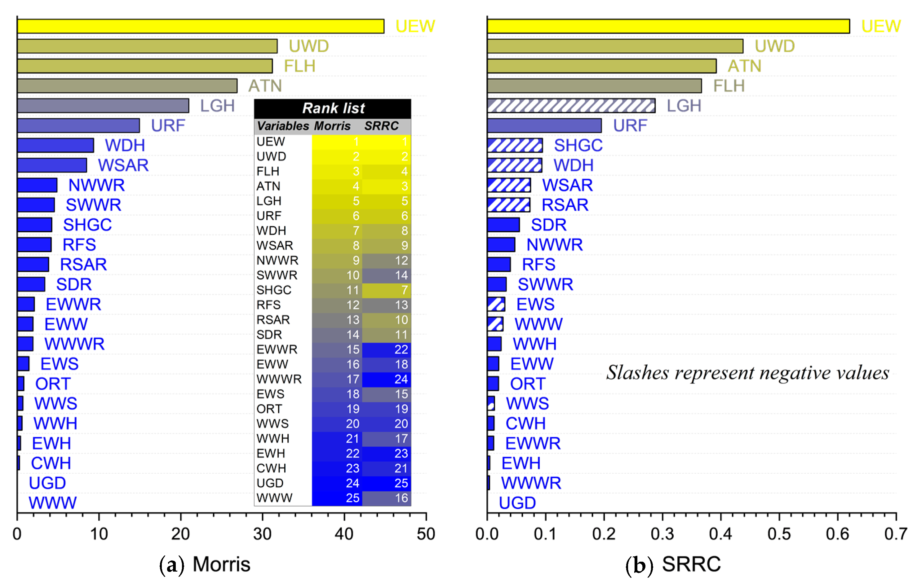
2.2.1. Stage 1: Morris and SRRC

In the initial stage, Morris and SRRC were used to preselect the relatively significant ones from a vast set of variables, thereby fixing or eliminating the minor ones. These two methods both have their own strengths in SA. Morris offers high operational efficiency and the ability to account for the interactions between input variables; SRRC is similarly computationally small and applicable to the nonlinear monotonic functions between inputs and outputs. However, neither can exactly quantify the variance of the output for various input elements, and the aim of the pairing is to synthesize and identify which input variables have a major impact on the output uncertainty of the high-dimensional models. Morris has two evaluation indicators: μ is used to assess the primary effect of the input on the output, while σ can be employed to determine the interaction of the parameters with nonlinear response. The primary computational process of Morris can be expressed as [5,20,34]:
E E i = y ( x + e i Δ i ) y ( x ) Δ i ,
μ i = 1 r i = 1 r E E i ,
σ i = 1 ( r 1 ) i = 1 r ( E E i μ i ) ,
where E E i represents the elementary effect to determine the effect of input variations on outputs; y ( x ) and y ( x + e i Δ i ) represent the model outputs before and after input variations, respectively; e i is zero vector; Δ i is variation value of x i ; μ i and σ i are mean value and standard deviation, respectively.
Regression-based methods have numerous types, all of which establish the correlation between inputs and outputs by modeling the mathematical expressions, but with different application conditions. Therefore, the correlation of the independent variables and the monotonic nonlinearity of the model need to be determined well in advance before it starts formally working. SRRC was employed in this paper, with its pre-processing discussed in more detail in Section 4.1.

2.2.2. Stage 2: Sobol Indices

In the second stage, the effect of the inputs on the outputs was quantitatively evaluated using the even more robust Sobol, which not only quantifies the output variances due to each of the inputs, but also takes into account the interactions between the variables. Nevertheless, it requires mutually independent inputs and a high sample size to ensure model convergence, dramatically increasing the computational effort. That is the key benefit of setting Stage 1. The Sobol results consist of the first-order effect and total effect indices of the variables. The variance-based SA are premised on decomposing a square integrable mathematical function into [35,36]:
Y ( x ) = Y 0 + i k Y i ( x i ) + i < j k Y i j ( x i , x j ) + + Y 12 k ( x 1 , x 2 x k ) ,
where Y 0 is a constant; x i represents an input.
The total model variance V ( Y ) can be decomposed into the variance generated by the independent action and the joint effect of parameters [37]:
V ( Y ) = i V i + i < j V i j + + V 12 k ,
where V i denotes the effect of the i   t h input to the output; V i j and V 12 k are the effect of the interactions between two inputs and k inputs on the output.
Thus, the first-order effect that reflects the contribution of x i to the total variance of Y can be expressed as S i , which is an estimate of the expected variance fraction in the model output [37]:
S i = V i V ( Y ) ,
For both sides of Equation (5) divide simultaneously by V ( Y ) to be able to find i S i ≤ 1, where i S i = 1 for linear and additive models:
1 = i S i + i < j S i j + + S 12 k ,
Further, the total effect indices S T i can be calculated as [38]:
S T i = S i + S i j + S 12 k = 1 V ~ i V ( Y ) ,

3. Case Study

3.1. Control Variables and Parameters

Rural and urban housing share distinctly different patterns in terms of both design and use. Consequently, the design lessons of urban buildings cannot be transferred to rural ones. From nine villages in the cold IIB region of China, 150 units were studied in the field to bring the findings as close to practice as possible. Details on this work can be found in Appendix A. By field research and literature review [31,39,40,41], 25 variables were identified for SA, where No. 1–13 refer to the spatial parameters while No. 14–25 refer to the envelope parameters. All variables were set as uniformly distributed continuous data. The abbreviated names, intervals, and reference values of each variable follow in Table 2. The reference value comes close to the mean of the actual measured parameters of CSDs.

3.2. Parametric BEM

Single-story CSDs of L-shaped and U-shaped layouts were designated for the research, which could be interchanged by adapting the dimensions of the wings. The BEM built with Rhino & Grasshopper was used to estimate the annual heating and cooling demands, with heating and cooling setpoints at 15 °C and 26 °C, respectively. The occupant density was 0.1 person/m2, and the occupancy rate as indicated in Figure 3. The lighting power density was set to 4.0 W/m2 which remained on between 6:00–8:00 and 18:00–22:00. Other less-used devices dissipating heat were neglected. The calculated U-values of the interior walls and ceilings were 1.72 W/m2K and 1.62 W/m2K, respectively. The U-values of the interior walls and ceilings, roughly calculated by layers and material properties, were 1.72 W/m2K and 1.62 W/m2K, respectively.

4. Results and Discussion

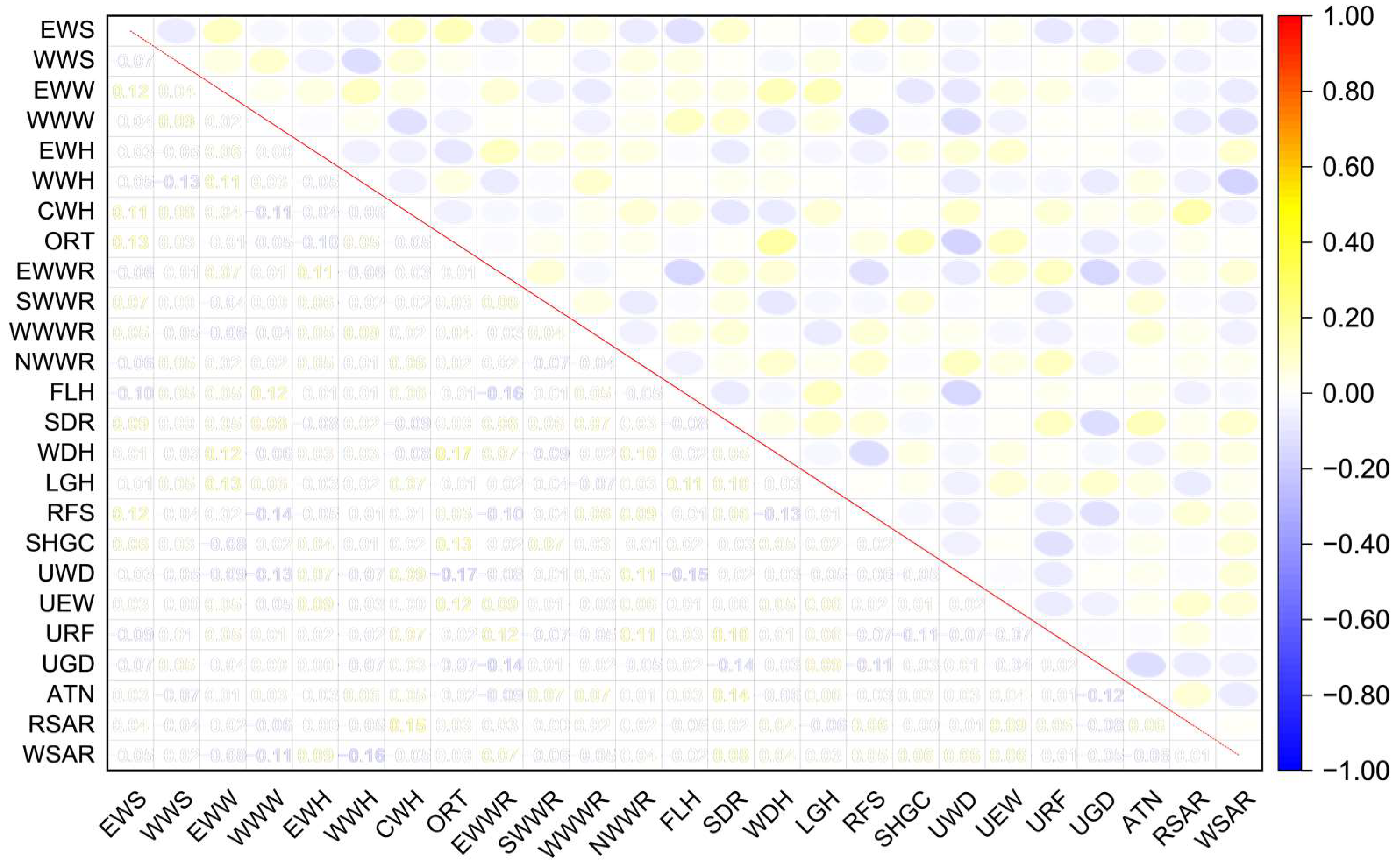
4.1. Parameters Screening by SRRC & Morris

The parameter correlation and model nonlinearity always dictate the selection of SA methods, especially the regression-based method. Therefore, the monotonicity of the model needs to be determined first to ascertain the validity of the method. A parametric sweep of 25 variables using the OAT approach yields the fluctuation trend of energy demand as shown in Figure 4. Definitively, the outputs maintained monotonically vary to different inputs, without extreme points within the interval, which could provide the basis for the subsequent SA method selection.
The correlations between the inputs, as shown in Figure 5, were identified with the Pearson correlation coefficient. The entire graph was shaded extremely faintly, indicating that the variables had very weak mutual correlations. The elliptical direction of the upper triangle indicated the positive and negative correlations between the variables, and the bottom triangle gave the precise values. The overwhelming majority of the variables had correlation coefficients with absolute values less than 0.1, while a small minority were also below 0.2. It suggested that the variables were so weakly correlated that they could be regarded as uncorrelated. Thus, for the regression-based method, SRC and SRRC could be initially identified as the applicable SA methods for this study. For further examination of the approach validity, whether the model was linear or not was then discussed, and a linear regression study of 25 variables versus annual cooling and heating demands was conducted. It was evident that the linear correlation of annual energy demand with variables was less robust (R2 = 0.51 for cooling demand; R2 = 0.62 for heating demand), that is, only 51% of the cooling demand data and 62% of the heating demand data could be linearly explained with the inputs. Furthermore, the p-values of cooling and heating demands were 4.89 × 10⁻²⁵ and 2.19 × 10−44, respectively, which were both far below 0.001. Therefore, a significant nonlinear correlation could be concluded between the inputs and outputs. To sum up, SRRC and Morris were used as the mutually complementary SA methods at the first stage to screen the significance parameters rationally.
With regard to cooling demand, Figure 6 shows the sensitivity rankings of the variables presented by Morris and SRRC. Surprisingly, the two SA methods exhibited fairly consistent results on this issue. From the 25 parameters, the top 12 highly sensitive parameters were sorted out and used as the inputs for the subsequent SA rounds, namely RSAR, ATN, FLH, WSAR, SHGC, UEW, LGH, NWWR, WWWR, EWWR, SDR, WDH. Despite that, the rankings of the 12 parameters still differed slightly between the two methods. First, the shading ratio was the most sensitive variable in terms of the spatial parameters, except for the width, the depth, and the floor height. It was once speculated that the presence of wings and fences in courtyard houses might interfere with the solar absorption of the principal building and thus the energy demand. However, apparently, the dimensional parameters concerning the courtyard fences and the wings, inclusive of the spacing between the wings and the principal building, were identified as secondary parameters ranked in the bottom ten. The phenomenon most likely arose because these variables even when taken to the boundary values, still could not shade the principal building: in fact, the heights of the wings and fences were less than the floor heights of the principal building and the wings had a distance of 1 m closest to the principal building. Then it also suggested that in certain higher latitudes, the sensitivity rankings of these parameters might shift forward. The impact of south-side window-to-wall ratio was less significant than that of the north-side one due to the sun-shading effect, while the highest influential factor was found on the east–west side. Second, in terms of envelope parameters, the U-value ranked high as expected, but only for those of exterior walls, while those of other parts such as exterior windows, roofs, and floors showed only limited significance. Compared to the U-value, the radiation properties of the envelope had a more significant effect on cooling demand. The solar absorptivity of roofs and façades as well as SHGC ranked in the top five by both methods. The impact of envelope parameters on cooling demand tended to be more significant than that of spatial ones, owing to the pronounced role of solar heat gain on building cooling.
Several of the previous patterns were retained for the heating demand, but there were a few differences. Figure 7 shows the sensitivity ranking of the variables for the heating energy consumption presented by Morris and SRRC. Both methods consistently identified 14 highly sensitive parameters, which, as expected, still had slightly different rankings. The inputs screened for the second SA round consisted of UEW, UWD, ATN, FLH, LGH, URF, SHGC, WDH, WSAR, SDR, NWWR, SWWR, RSAR, RFS. Roof slope was the spatial parameter that had a significant effect on the heating demand in addition to the four aforementioned sensitive variables. The previous situation was reversed in terms of envelope parameters: the heat transfer coefficient became the primary significant parameter. At this point, the heat transfer coefficients of either exterior walls, exterior windows, or roofs exerted a strong impact on the heating demand. The reason for such a result might be that radiation was relatively weak in winter, while the indoor–outdoor temperature difference was much larger than that in summer, so the heat transfer driven by the temperature difference would be even greater if the thermal resistance of the large area of the envelope was poor. In addition, the airtightness of the building had a remarkable impact on heating demand. Similar to the results for cooling demand, the spatial parameters had a minor impact on energy consumption compared to the envelope ones.

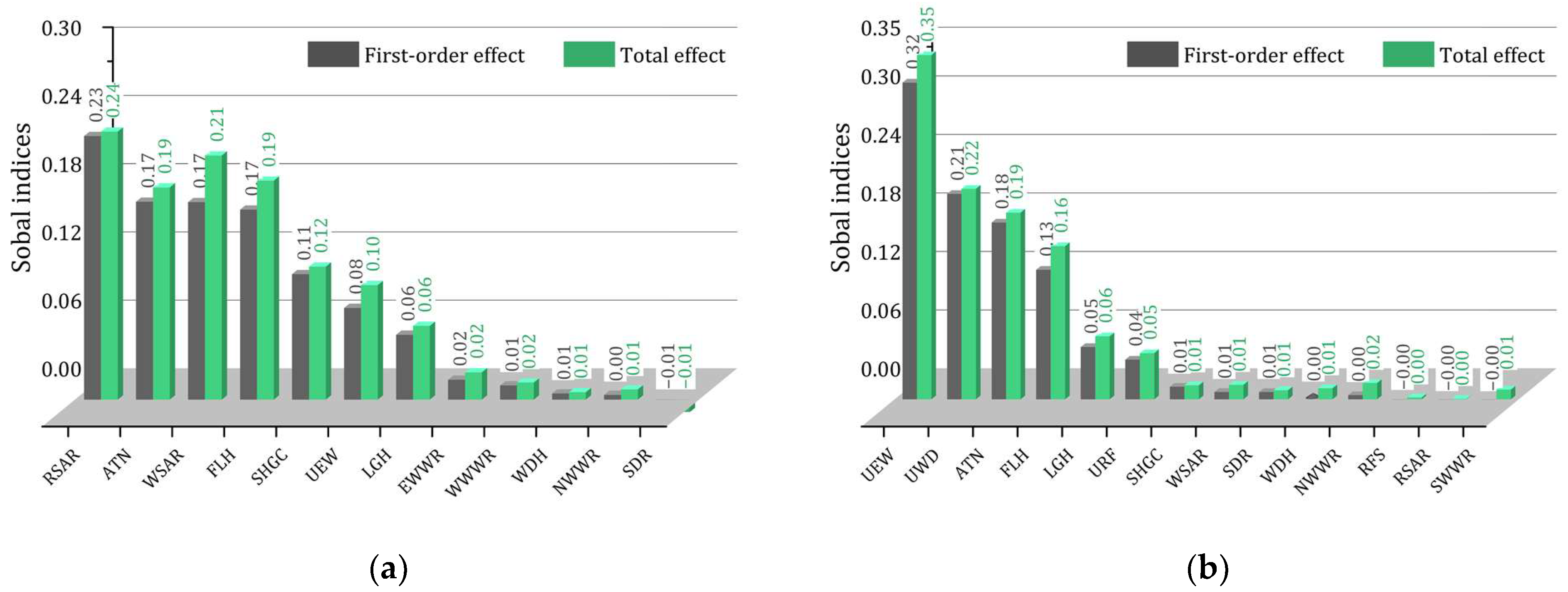
4.2. Quantitative Analysis by Sobol

From the initial SA screening, 12 and 14 significant parameters remained on cooling and heating demands, respectively. Although both Morris and SRRC gave superior sensitivity rankings for these variables in their SA results, the rankings within these variables differed. To rectify this deficiency and to quantify the sensitivities more precisely, Sobol, a variance-based method, was used in the second-stage SA.
Figure 8 shows the distributions of the cooling and heating demands corresponding to the 3328 sample sets, which were attempted to be depicted as lognormal vs. normal. The cooling demand was positively skewed, and its values were concentrated in the interval 27.4, 45.3. At this point, the geometric mean μg was 34.9 ± 0.2 kWh/m2 ranging from 21.7 kWh/m2 to 64.6 kWh/m2, which indicated the significant effect of these 12 parameters on cooling demand. Likewise, the heating demand also showed a positive skewed distribution whose values concentrated at the interval 30.3, 87.1. At this point, the geometric mean μg was 53.1 ± 1.2 kWh/m2 ranging from 12.2 kWh/m2 to 135.9 kWh/m2, suggesting that the effect of these 14 parameters on the heating demand was considerable. Then, the normal Q-Q plot revealed that the cooling and heating demands could meet the normal distribution. The mean values of cooling and heating demands μ were 37.1 kWh/m2 and 62.5 kWh/m2 respectively at that time, with the standard deviation σ of 6.9 and 21.1, respectively.
Figure 9 indicates the first-order effect indices (S1) and the total effect indices (St) obtained by Sobol. Among the parameters that had a significant effect on the annual cooling demand, those concerning the solar absorptivity of the envelope occupied three of the top five. The solar absorptivity of roofs and facades as well as SHGC could induce variations in cooling demand of 23.2%, 17.4%, and 11.7% (52.3% in total), respectively. Meanwhile, the airtightness, the floor height, and the heat transfer coefficient of the exterior wall were also parameters not to be ignored, which were capable of causing 17.4%, 16.7%, and 8.1% (42.2% in total) variations in cooling energy consumption independently. The sensitivity of the cooling demand to the solar absorptivity of the facade increased by 4% when the interaction of other parameters was considered. In addition, the floor height, the U-value of exterior walls, and the airtightness were also significantly affected by the interaction, while the other parameters showed little difference. Out of the significant parameters affecting the annual heating demand, the U-value and airtightness of the envelope were the most prominent. The U-value of exterior walls and windows as well as the airtightness could induce 32.5%, 21.1%, and 18.1% (71.7% in total) variations in heating demand separately. Similar to the cooling demand, the floor height had considerable sensitivity to heating demand, which acted alone to induce a 13.3% variation in heat demand. Regarding the parameter interaction, except for the heat transfer coefficient of the exterior windows and the floor height, the S1 and St of the remaining parameters were quite similar, that is, the variability of the parameter sensitivity due to the interaction was not considerable.
The Sobol method had been proven to be the most accurate of the three methods in previous studies [38,42]. In this study, it was also easy to find the conclusion differences between the three methods given, as shown in Table 3. Out of the 12 significant variables for cooling demand, the three methods consistently provided the top five parameters, even if their rankings differed somewhat. The sensitivity ranking of the parameters was essentially the same for SRRC compared to S1, where their maximum ranking difference did not exceed two. Since the interaction between these 12 parameters was not very prominent, similar findings could be found in the comparison of SRRC vs. St., while Morris yielded a three-position difference in rankings compared to Sobol. As can be seen, although Morris could effectively screen most of the significant parameters, its ranking of parameter sensitivity was not yet quite robust, for which one potential solution was to expand the sample size. Among the 14 significant variables for heating demand, the three methods were in general agreement in determining the top six parameters in the sensitivity ranking. For these six parameters, SRRC agreed exactly with the ranking given by Sobol, while Morris presented the different one for ATN and FLH. For the latter eight parameters in the sensitivity ranking, SRRC was relatively close to the conclusion reached by S1, while Morris fully underestimated the significant effect of SHGC on heating demand in the process. In general, the ranking discrepancy between SRRC, Morris, S1, and St could be attributed to two main aspects: (1) the mis-ranking of the not significant parameters might be because their sensitivity indices were so small that the absolute differences were negligible; (2) the ranking discrepancy between St and the others might be due to the fact that the sensitivity indices themselves were small enough that although the interaction was not obvious, it was sufficient to shift the sensitivity ranking of those parameters.

5. Energy Prediction and Optimization Study

5.1. Prediction Model Description

Building energy simulations tend to require a vast number of complex inputs, requiring substantial effort to access and difficult to control uncertainty. SA helps the designer to exclude a large amount of secondary information and thus obtain a highly accurate output by the saliency parameters alone, which supports the design aspects that need to be adjusted iteratively to optimize the building performance. Here in this section, the prediction model of cooling and heating demands was developed based on the significant parameters identified in the previous study. Several assumptions should be stated in advance to ensure the model validity: (1) the experimental building form could be approximately described by the established model as in Figure 3; (2) the parameter ranges of the experimental building could be contained in or approximated to those of the established model; (3) the fixed parameters in the model building, such as heating and cooling setpoints, user schedules, etc., could describe closely the actual situation; (4) the meteorological conditions should be consistent with or similar to those of the established model.
Gaussian Process Regression (GPR) was used to train prediction models, which were typically appropriate for addressing nonlinearities. Since the GPR achieved prediction by the very process of probabilistic inference, it was capable of quantifying the prediction uncertainty in a principled way. However, the drawback of GPR was that as a non-parametric model, its computational complexity surged with the volume of data; specifically, for N samples, it would have a complexity of O (N3), exactly the problem solved by the previous SA. Likewise, Support Vector Machine (SVM), Random Forest (RF), and Multi-layered Perceptron (MLP) were all recognized as excellent prediction algorithms; thus they were used to verify the training precision. In addition, Linear Regression (LR) was employed to compare the results with the machine learning algorithms.

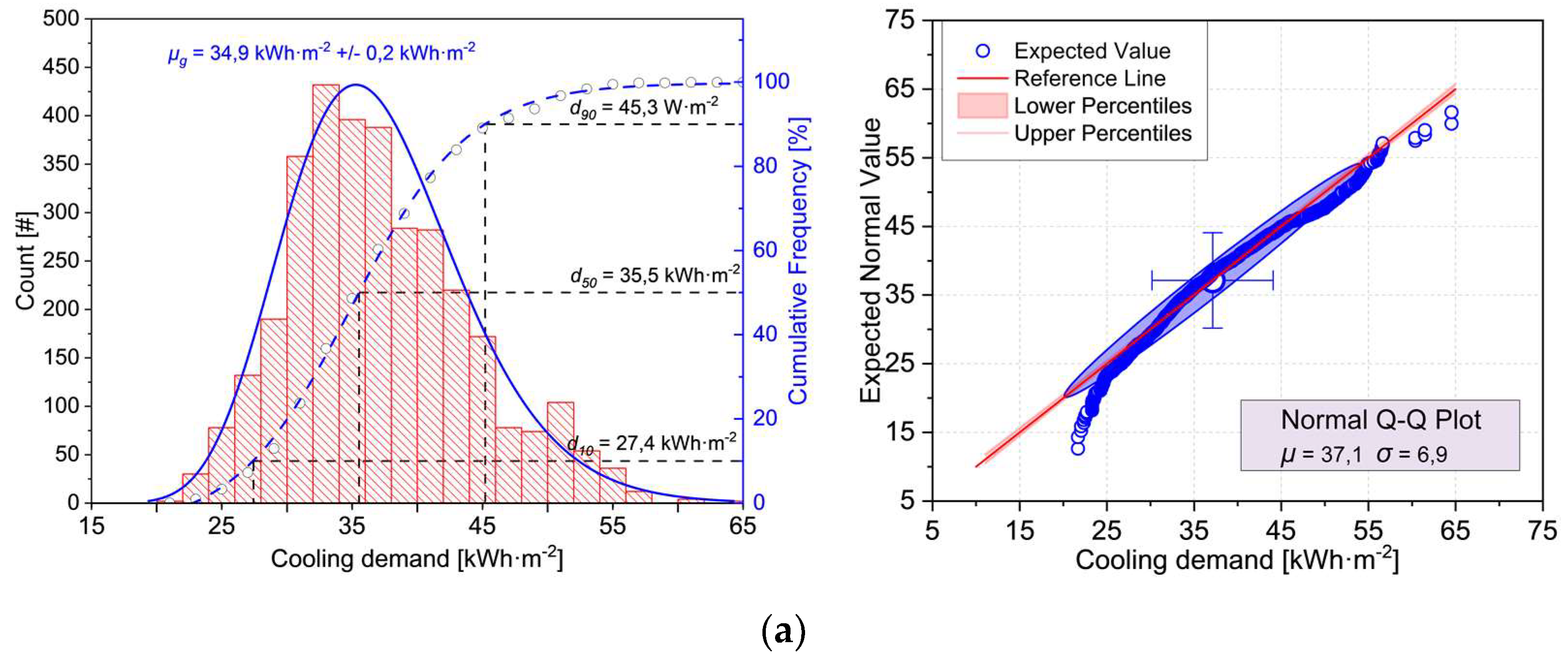
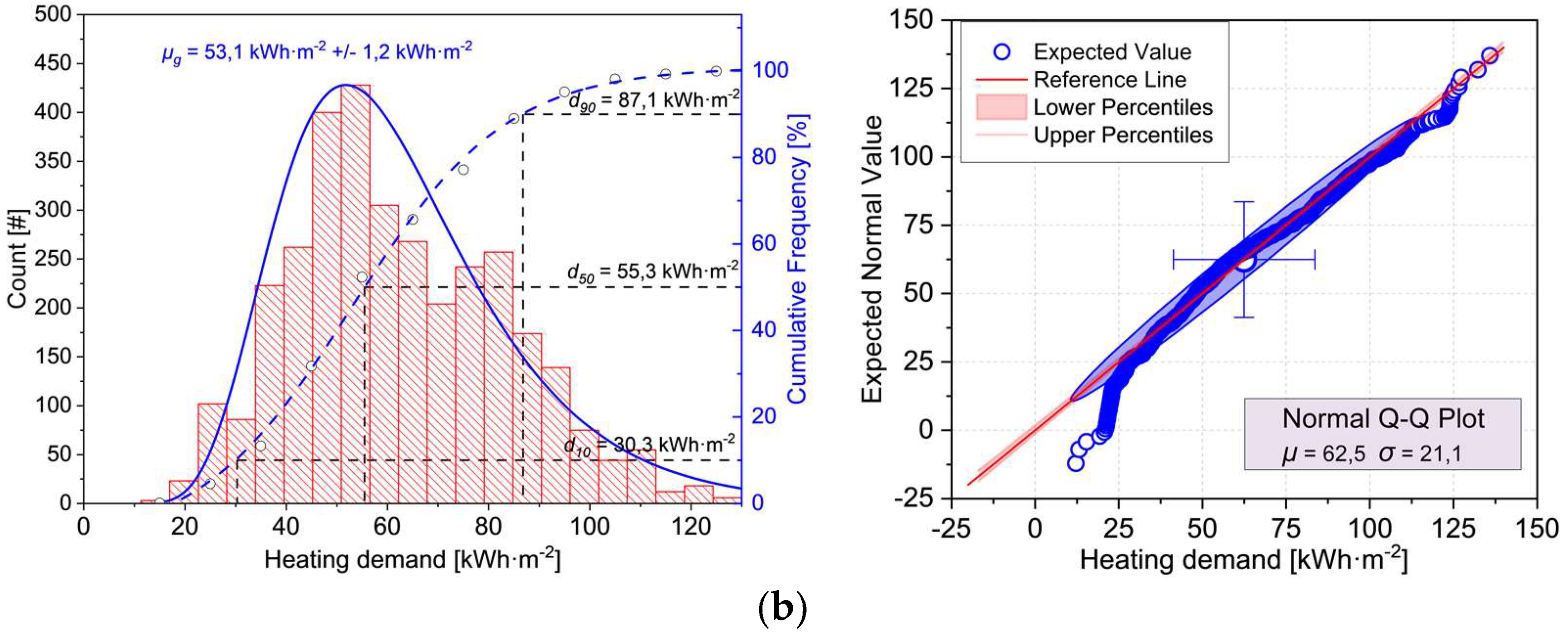
5.2. Model Performance Evaluation

During the model training, the significant parameters with St larger than 0.04 were retained, namely RSAR, WSAR, FLH, ATN, SHGC, UEW, LGH, UWD, and URF. The GPR model was trained and tested with 10 cross-validation folds based on a set of 7122 samples. Several factors might affect the accuracy of GPR models, such as basis function, kernel function, kernel scale, sigma, etc., which gave difficulty in specifying artificially the optimal or near-optimal values. Thus, Bayesian optimization was employed to identify the specific values of the hyperparameters so as to obtain a highly accurate GPR model. At this point, the acquisition function was set as expected improvement per second plus and the signal standard deviations of the energy demand models were predefined as 4.91 and 14.95, respectively. Table 4 shows the optimized hyperparameters of the GPR model as well as their search range. Eventually, the optimization process for both the cooling demand and heating demand models went through 30 iterations. Figure 10 shows the optimizable GPR models and their prediction results for energy. From the results, it could be seen that the accuracy of the model was significantly improved by optimization, with good consistency between the predicted and actual values, and the residuals could be kept within an acceptable range.
A comparative experiment was conducted using linear regression and machine learning algorithms (including SVM, RF, and MLP) to further evaluate the prediction accuracy of the GPR model. The specific configurations of these algorithms are shown in Table 5, and the performance of all these algorithms was compared with 10-fold cross-validation. Figure 11 is a box plot comparing the prediction residuals of the models derived from GPR vs. LR and three machine learning algorithms. As we can see, the residuals of all five models were well controlled, with the absolute value of the residuals distributed below three for the vast majority of the data. However, whether for predicting cooling or heating demand, the GPR model remained the best performance among these models. For cooling demand prediction, the RMSEs of each model were ranked as LR (2.7564) > MLP (1.9426) > SVM (1.5231) > RF (1.5109) > GPR (1.2901). Similarly, in heating demand, the RMSE ranking of the models was LR (4.8936) > MLP (3.5804) > RF (3.3442) > SVM (2.8163) > GPR (2.3259).

5.3. Optimization

In this part, optimal design was used as an instance of the advanced usage of prediction models. Naturally, the main purpose of this paper would be to provide decision support for the design of CSDs, thus the optimization was centered on minimizing the total annual energy demand with the above screened sensitive parameters. On this basis, construction cost was introduced as the second objective, which in turn led to a dual-objective optimization for the nine parameters. Here, the construction cost was assumed to conform to a linear function, fitted by the collected data during field research. The optimization process was performed based on the Nondominated Sorting Genetic Algorithm III (NSGA-III). The crossover fraction was set to 0.8, and the population size and stall generation limit were set to 200 and 500, respectively. Figure 12 illustrates the final optimization result. The random data shown in Figure 12 were the output solutions corresponding to the random matrix generated with the rand function following the interval of nine variables for verifying the reliability of the Pareto front.
After the dual-objective optimization, 80 sets of optimal combinations regarding the nine variables were obtained. To comprehensively evaluate and compare their technical economy (TE), the definition of RB was introduced as:
R B = { E avg E opt C opt C avg , E avg > E opt 0 , E avg < E opt ,
where Eavg and Eopt represent the mean energy demand of the random matrix output and the energy demand of the Pareto front, respectively; Similarly, Cavg and Copt are the mean cost of the random matrix output and the cost of the Pareto front, respectively.
When using RB for evaluation, the larger its value indicates that the solution would yield better energy investment benefits, and solutions without energy conservation effect were excluded as zero. Figure 13 gives a comparative evaluation of the 80 optimal parameter sets. From the selected optimal TE solutions, it could be found that most of the variables were not completely biased towards the interval boundaries. The bias of the optimal variables towards the interval boundary might be explained in two reasonable ways: (1) the additional investment in the variable exceeded the improvement in energy efficiency by a large margin; (2) the same energy objective could be achieved more efficiently by adding investments to other variables. Therefore, it could be believed that the specific state of the optimal solution depended heavily on the mutual response between the two objective functions, which indicated that the uncertainty of the objective function would significantly cut the generalizability of the optimal solution. Nevertheless, the resulting Pareto front could still preserve its learning value for design decisions.

6. Conclusions

The present research set out to organize a GSA-based workflow for the optimal design of CSDs in cold regions of China. This workflow comprised several fragmentation processes such as UA, GSA, energy prediction model regression, and multi-objective optimization. First, the principles and characteristics of the four prevailing SA methods were reviewed and identified. Second, the uncertainty of energy demand to parameters and the sensitivity ranking of parameters were acquired by the sequential SA with Morris, SRRC, and Sobol. Third, a GPR model capable of predicting the annual energy demand was trained and outperformed in comparison with the accuracy of LR, SVM, RF, and MLP. Fourth, based on the obtained prediction models, an optimal design of the case building with a dual objective of energy and economy was accomplished by using NSGA-III. These efforts provide a relatively complete and robust strategy to support the CSD design, screening nine significant parameters on energy demand to aid qualitative optimization, as well as a set of 80 techno-economically sound Pareto front solutions for quantitative strategies. Further, the GSA-based optimization workflow ties the above fragmented studies into a logical sequence, offering a framework for further depth and richness in each area of research.
One limitation of this study lies in the insufficient sample size, which may make these findings less generalizable to CSDs in each region. For practical analytical reasons, it is quite challenging to retrieve the perfect parameter intervals and to fit the full range of cost data, which will lead to a certain bias of the final Pareto front. To remedy this deficiency, the research samples were persistently expanded to cover as much information as possible, even though this entails a substantial cost, which in fact will still take quite a bit of time for the vast size of China. Despite its limitations, the study certainly adds to our understanding of the problems of energy-saving design strategy support of CSDs, which would be a fruitful area for further work. Thus, greater efforts might be needed to expand the scope of application as follows: (a) Developing a plug-in for real-time parameter adjustment—a python-based framework is under development to address the dependency of multiple fragmented studies of this workflow on their respective software platforms, and in the near future, the workflow could be easily available to architects as a plug-in of grasshopper; (b) Refining more efficiency–accuracy balanced sequential SA methods—the hybrid SA approach can effectively integrate the merits of various SA methods, of which the sequential SA method with Morris/SRRC and Sobol proposed in this paper is just one, and numerous other possible rational hybrid methods deserve to be explored; (c) Establishing a set of constantly improving rural housing databases—our team is persisting with extensive field research and statistics on rural building data in cold regions of China, covering the construction historical information, building prototype clustering, occupant behavior data, construction cost statistics, etc. This work serves as a data basis for the replication of more generalized findings.

Author Contributions

Conceptualization, J.G. and Y.J.; methodology, Y.J.; software, C.S. and Y.J; formal analysis, Y.J. and M.L.; data curation, C.S. and Z.W.; writing—original draft preparation, Y.J.; writing—review and editing, J.G. and Y.J.; supervision, J.G.; funding acquisition, J.G. All authors have read and agreed to the published version of the manuscript.

Funding

This work was funded by the National Key R & D Program of China, Grant Number 2019YFD1101004.

Institutional Review Board Statement

Not applicable.

Informed Consent Statement

Not applicable.

Data Availability Statement

Not applicable.

Conflicts of Interest

The authors declare no conflict of interest.

Abbreviations

BPABuilding performance analysis
SASensitivity analysis
LSALocal sensitivity analysis
GSAGlobal sensitivity analysis
OATOne-parameter-at-a-time
BEMBuilding energy model
SHGCSolar heat gain coefficient
SRCStandard Regression Coefficients
PCCPartial Correlation Coefficients
SRRCStandardized Rank Regression Coefficients
PRCCPartial Rank Correlation Coefficients
UAUncertainty analysis
CSDCourtyard-style dwelling
S1First-order effect indices
StTotal effect indices
GPRGaussian Process Regression
SVMSupport Vector Machine
RFRandom Forest
MLPMulti-layered Perceptron
LRLinear Regression
NSGA-IIINondominated Sorting Genetic Algorithm III
TETechnical economy

Appendix A

Figure A1. Basic characteristics of field research samples: (a) building location; (b) construction age; (c) floor count; (d) total cost; (e) user count; (f) production mode.
Buildings 12 01132 g0a1
Figure A2. Common courtyard layout of CSDs in the survey: (a) I-shaped; (b) II-shaped; (c) L-shaped; (d) U-shaped.
Buildings 12 01132 g0a2
Table A1. Common enclosure structure form of rural houses in the survey.
TypeMain MaterialConstruction Layer (Inside Out)
Layer 1Layer 2Layer 3
Exterior wallClay brickGypsum/PVCMain structure
(Without insulation)
Mortar/Tile/Vacant
Hollow blockGypsum/PVCMortar/Tile/Vacant
AdobeWrapped clay brick/
Choi steel/Vacant
Gypsum
RoofHollow slab/
Concrete slab
Main structure
(Without insulation)
Cinder limeTile/Vacant
Tile/Choi steel/
WindowSingle glassCurtain/VacantWood/PVC/Aluminum alloy/Bridge-cut-off aluminum alloyPlastic cloth/Vacant
Double glass
DoorWood/Stainless steel /Aluminum alloyMain structureCurtain/

References

  1. Hensen, J.; Lamberts, R. Building Performance Simulation for Design and Operation; Taylor & Francis: Abingdon, UK, 2011; ISBN 978-0-415-47414-6. [Google Scholar]
  2. Saltelli, A. Sensitivity Analysis in Practice: A Guide to Assessing Scientific Models; Wiley: Hoboken, NJ, USA, 2004; ISBN 978-0-470-87093-8. [Google Scholar]
  3. Iooss, B.; Lemaître, P. A Review on Global Sensitivity Analysis Methods. arXiv 2014, arXiv:1404.2405. [Google Scholar]
  4. Hamby, D.M. A Review of Techniques for Parameter Sensitivity Analysis of Environmental Models. Environ. Monit. Assess. 1994, 32, 135–154. [Google Scholar] [CrossRef]
  5. Kristensen, M.H.; Petersen, S. Choosing the Appropriate Sensitivity Analysis Method for Building Energy Model-Based Investigations. Energy Build. 2016, 130, 166–176. [Google Scholar] [CrossRef]
  6. Xu, C.; Gertner, G. Understanding and Comparisons of Different Sampling Approaches for the Fourier Amplitudes Sensitivity Test (FAST). Comput. Stat. Data Anal. 2011, 55, 184–198. [Google Scholar] [CrossRef] [PubMed] [Green Version]
  7. Goffart, J.; Woloszyn, M. EASI RBD-FAST: An Efficient Method of Global Sensitivity Analysis for Present and Future Challenges in Building Performance Simulation. J. Build. Eng. 2021, 43, 103129. [Google Scholar] [CrossRef]
  8. Neale, J.; Shamsi, M.H.; Mangina, E.; Finn, D.; O’Donnell, J. Accurate Identification of Influential Building Parameters through an Integration of Global Sensitivity and Feature Selection Techniques. Appl. Energy 2022, 315, 118956. [Google Scholar] [CrossRef]
  9. Paleari, L.; Movedi, E.; Zoli, M.; Burato, A.; Cecconi, I.; Errahouly, J.; Pecollo, E.; Sorvillo, C.; Confalonieri, R. Sensitivity Analysis Using Morris: Just Screening or an Effective Ranking Method? Ecol. Model. 2021, 455, 109648. [Google Scholar] [CrossRef]
  10. Wang, C.; Peng, M.; Xia, G. Sensitivity Analysis Based on Morris Method of Passive System Performance under Ocean Conditions. Ann. Nucl. Energy 2020, 137, 107067. [Google Scholar] [CrossRef]
  11. King, D.M.; Perera, B.J.C. Morris Method of Sensitivity Analysis Applied to Assess the Importance of Input Variables on Urban Water Supply Yield—A Case Study. J. Hydrol. 2013, 477, 17–32. [Google Scholar] [CrossRef]
  12. Zhao, J.; Zhang, J.J.; Grunewald, J.; Feng, S. A Probabilistic-Based Method to Evaluate Hygrothermal Performance of an Internally Insulated Brick Wall. Build. Simul. 2021, 14, 283–299. [Google Scholar] [CrossRef]
  13. Tøndel, K.; Vik, J.O.; Martens, H.; Indahl, U.G.; Smith, N.; Omholt, S.W. Hierarchical Multivariate Regression-Based Sensitivity Analysis Reveals Complex Parameter Interaction Patterns in Dynamic Models. Chemom. Intell. Lab. Syst. 2013, 120, 25–41. [Google Scholar] [CrossRef] [Green Version]
  14. Haahtela, T.J. Regression Sensitivity Analysis for Cash Flow Simulation Based Real Option Valuation. Procedia-Soc. Behav. Sci. 2010, 2, 7670–7671. [Google Scholar] [CrossRef]
  15. Li, X.; Li, L.; Yang, Y.; Zhao, G.; He, N.; Schmidt, E. Variance-Based Sensitivity Analysis for the Influence of Residual Stress on Machining Deformation. J. Manuf. Process. 2021, 68, 1072–1085. [Google Scholar] [CrossRef]
  16. Pohya, A.A.; Wicke, K.; Kilian, T. Introducing Variance-Based Global Sensitivity Analysis for Uncertainty Enabled Operational and Economic Aircraft Technology Assessment. Aerosp. Sci. Technol. 2022, 122, 107441. [Google Scholar] [CrossRef]
  17. Chen, X.; Yang, H.; Sun, K. Developing a Meta-Model for Sensitivity Analyses and Prediction of Building Performance for Passively Designed High-Rise Residential Buildings. Appl. Energy 2017, 194, 422–439. [Google Scholar] [CrossRef]
  18. Yun, W.; Lu, Z.; He, P.; Jiang, X.; Dai, Y. Parameter Global Reliability Sensitivity Analysis with Meta-Models: A Probability Estimation-Driven Approach. Aerosp. Sci. Technol. 2020, 106, 106040. [Google Scholar] [CrossRef]
  19. Zhao, Y.; Guo, Z.; Niu, F.; Yu, Y.; Wang, S. Global Sensitivity Analysis of Passive Safety Systems of FHR by Using Meta-Modeling and Sampling Methods. Prog. Nucl. Energy 2019, 115, 30–41. [Google Scholar] [CrossRef]
  20. Heiselberg, P.; Brohus, H.; Hesselholt, A.; Rasmussen, H.; Seinre, E.; Thomas, S. Application of Sensitivity Analysis in Design of Sustainable Buildings. Renew. Energy 2009, 34, 2030–2036. [Google Scholar] [CrossRef] [Green Version]
  21. Maučec, D.; Premrov, M.; Leskovar, V.Ž. Use of Sensitivity Analysis for a Determination of Dominant Design Parameters Affecting Energy Efficiency of Timber Buildings in Different Climates. Energy Sustain. Dev. 2021, 63, 86–102. [Google Scholar] [CrossRef]
  22. Tian, W.; de Wilde, P. Uncertainty and Sensitivity Analysis of Building Performance Using Probabilistic Climate Projections: A UK Case Study. Autom. Constr. 2011, 20, 1096–1109. [Google Scholar] [CrossRef]
  23. Yıldız, Y.; Arsan, Z.D. Identification of the Building Parameters That Influence Heating and Cooling Energy Loads for Apartment Buildings in Hot-Humid Climates. Energy 2011, 36, 4287–4296. [Google Scholar] [CrossRef] [Green Version]
  24. Spitz, C.; Mora, L.; Wurtz, E.; Jay, A. Practical Application of Uncertainty Analysis and Sensitivity Analysis on an Experimental House. Energy Build. 2012, 55, 459–470. [Google Scholar] [CrossRef]
  25. Shen, H.; Tzempelikos, A. Sensitivity Analysis on Daylighting and Energy Performance of Perimeter Offices with Automated Shading. Build. Environ. 2013, 59, 303–314. [Google Scholar] [CrossRef]
  26. Pang, Z.; O’Neill, Z.; Li, Y.; Niu, F. The Role of Sensitivity Analysis in the Building Performance Analysis: A Critical Review. Energy Build. 2020, 209, 109659. [Google Scholar] [CrossRef]
  27. Pang, Z.; O’Neill, Z. Uncertainty Quantification and Sensitivity Analysis of the Domestic Hot Water Usage in Hotels. Appl. Energy 2018, 232, 424–442. [Google Scholar] [CrossRef]
  28. Østergård, T.; Jensen, R.L.; Maagaard, S.E. A Comparison of Six Metamodeling Techniques Applied to Building Performance Simulations. Appl. Energy 2018, 211, 89–103. [Google Scholar] [CrossRef]
  29. Sun, H.; Leng, M. Analysis on Building Energy Performance of Tibetan Traditional Dwelling in Cold Rural Area of Gannan. Energy Build. 2015, 96, 251–260. [Google Scholar] [CrossRef]
  30. Tabadkani, A.; Aghasizadeh, S.; Banihashemi, S.; Hajirasouli, A. Courtyard Design Impact on Indoor Thermal Comfort and Utility Costs for Residential Households: Comparative Analysis and Deep-Learning Predictive Model. Front. Archit. Res. 2022, 1–18. [Google Scholar] [CrossRef]
  31. Soflaei, F.; Shokouhian, M.; Zhu, W. Socio-Environmental Sustainability in Traditional Courtyard Houses of Iran and China. Renew. Sustain. Energy Rev. 2017, 69, 1147–1169. [Google Scholar] [CrossRef]
  32. Wang, F.; Liu, Y. Thermal Environment of the Courtyard Style Cave Dwelling in Winter. Energy Build. 2002, 34, 985–1001. [Google Scholar] [CrossRef]
  33. Deng, Q.; Wang, G.; Wang, Y.; Zhou, H.; Ma, L. A Quantitative Analysis of the Impact of Residential Cluster Layout on Building Heating Energy Consumption in Cold IIB Regions of China. Energy Build. 2021, 253, 111515. [Google Scholar] [CrossRef]
  34. Loeppky, J.L.; Sacks, J.; Welch, W.J. Choosing the Sample Size of a Computer Experiment: A Practical Guide. Technometrics 2009, 51, 366–376. [Google Scholar] [CrossRef] [Green Version]
  35. Sobol, I.M. Global Sensitivity Indices for Nonlinear Mathematical Models and Their Monte Carlo Estimates. Math. Comput. Simul. 2001, 55, 271–280. [Google Scholar] [CrossRef]
  36. Mara, T.A.; Tarantola, S. Application of Global Sensitivity Analysis of Model Output to Building Thermal Simulations. Build. Simul. 2008, 1, 290–302. [Google Scholar] [CrossRef] [Green Version]
  37. Saltelli, A.; Annoni, P.; Azzini, I.; Campolongo, F.; Ratto, M.; Tarantola, S. Variance Based Sensitivity Analysis of Model Output. Design and Estimator for the Total Sensitivity Index. Comput. Phys. Commun. 2010, 181, 259–270. [Google Scholar] [CrossRef]
  38. Homma, T.; Saltelli, A. Importance Measures in Global Sensitivity Analysis of Nonlinear Models. Reliab. Eng. Syst. Saf. 1996, 52, 1–17. [Google Scholar] [CrossRef]
  39. Zheng, H.; Long, E.; Cheng, Z.; Yang, Z.; Jia, Y. Experimental Exploration on Airtightness Performance of Residential Buildings in the Hot Summer and Cold Winter Zone in China. Build. Environ. 2022, 214, 108848. [Google Scholar] [CrossRef]
  40. Lu, Y.; Xiang, Y.; Chen, G.; Liu, J.; Wang, Y. On-Site Measurement and Zonal Simulation on Winter Indoor Environment and Air Infiltration in an Atrium in a Severe Cold Region. Energy Build. 2020, 223, 110160. [Google Scholar] [CrossRef]
  41. Evans, M.; Yu, S.; Song, B.; Deng, Q.; Liu, J.; Delgado, A. Building Energy Efficiency in Rural China. Energy Policy 2014, 64, 243–251. [Google Scholar] [CrossRef]
  42. Yang, S.; Tian, W.; Cubi, E.; Meng, Q.; Liu, Y.; Wei, L. Comparison of Sensitivity Analysis Methods in Building Energy Assessment. Procedia Eng. 2016, 146, 174–181. [Google Scholar] [CrossRef] [Green Version]
Figure 1. Performance differences and characteristics of each SA method in six aspects.
Buildings 12 01132 g001
Figure 2. Flow chart of sensitivity analysis and subsequent research.
Buildings 12 01132 g002
Figure 3. Parametric building energy model with geometric variables and the floor plan of the case: (a) parametric BEM; (b) occupancy rate.
Buildings 12 01132 g003
Figure 4. Fluctuation trend of energy demand with 25 variables.
Buildings 12 01132 g004
Figure 5. The correlation between 25 variables expressed by Pearson correlation coefficient.
Buildings 12 01132 g005
Figure 6. Ranking of sensitivity parameters to cooling demand obtained by the two methods in the first-stage SA: (a) Morris (left); (b) SRRC (right).
Buildings 12 01132 g006
Figure 7. Ranking of sensitivity parameters to heating demand obtained by the two methods in the first-stage SA: (a) SRRC; (b) Morris.
Buildings 12 01132 g007
Figure 8. Frequency distribution of cooling and heating demands and normal Q-Q plot: (a) cooling demand; (b) heating demand.
Buildings 12 01132 g008aBuildings 12 01132 g008b
Figure 9. First-order effect indices (S1) and total effect indices (St) of sensitivity parameters to energy demand obtained by the Sobol method in the second-stage SA: (a) cooling demand; (b) heating demand.
Buildings 12 01132 g009
Figure 10. Energy prediction model trained by optimizable GPR with 10 cross-validation folds through 30 iterations: (a) cooling demand; (b) heating demand.
Buildings 12 01132 g010
Figure 11. The comparison on the accuracy of 10-fold cross validation using linear regression and machine learning: (a) cooling demand; (b) heating demand.
Buildings 12 01132 g011
Figure 12. Pareto front generated by NSGA-III dual-objective optimization and target distribution generated by 9–10,000,000 random matrix.
Buildings 12 01132 g012
Figure 13. Evaluation and comparison of the technique-economy of 80 optimal parametric combinations by using RB.
Buildings 12 01132 g013
Table 1. The sampling type and scale specified by different SA methods in different stages.
SA MethodSampling TypeSampling SizeCalculation Method
(K as Custom Factor)
SRRCLatin Hypercube Sampling250 (K = 10)K · N, K ≥ 10 [34]
MorrisMorris Sampling216 (K = 8)K · (N + 1), K = 4, 6, 8….
SobolSobol Sampling3328 for cooling (>2600 when K = 100)
3328 for heating (>3000 when K = 100)
K · (2N + 2), K = 100, 200, 500…. [35]
Table 2. Extracted design variables and their details.
#VariableAbbr.IntervalRef. ValueUnit
1EastWingSpacingEWS[1.00, 4.00]2.50m
2WestWingSpacingWWS[1.00, 4.00]2.50m
3EastWingWideEWW[0.00, 4.50]3.60m
4WestWingWideWWW[0.00, 4.50]3.60m
5EastWingHeightEWH[2.80, 4.00]3.00m
6WestWingHeightWWH[2.80, 4.00]3.00m
7CourtyardWallHeightCWH[2.80, 4.00]3.00m
8OrientationORT[−45.00, 45.00]0.00deg
9FloorHeightFLH[2.80, 4.00]3.80m
10ShadingRatioSDR[0.20, 1.20]0.80/
11WidthWDH[11.00, 17.00]12.60m
12LengthLGH[4.50, 7.50]7.00m
13RoofSlope RFS[15.00, 45.00]30.00deg
14EastWindowWallRatioEWWR[0.00, 0.30]0.15/
15SouthWindowWallRatioSWWR[0.20, 0.50]0.40/
16WestWindowWallRatioWWWR[0.00, 0.30]0.15/
17NorthWindowWallRatioNWWR[0.00, 0.30]0.10/
18SolarHeatGainCoefficientSHGC[0.20, 0.50]0.35/
19U-valueofWindowsUWD[1.20, 5.00]4.00W/m2K
20U-valueofExteriorWallUEW[0.20, 2.00]1.50W/m2K
21U-valueofRoofURF[0.20, 1.70]1.50W/m2K
22U-valueofGroundUGD[0.40, 3.40]3.00W/m2K
23AirTightnessATN[0.17, 1.00]0.50h−1
24RoofSolarAbsorptionRateRSAR[0.10, 0.90]0.48/
25ExteriorWallSolarAbsorptionRateWSAR[0.10, 0.90]0.48/
Table 3. The difference comparison of parameter ranking of energy demand given by various methods in the sequential SA process.
Cooling DemandHeating Demand
Var.MorrisSRRCS1StVar.MorrisSRRCS1St
RSAR1111UEW1111
WSAR4432UWD2222
FLH3343ATN4333
ATN2224FLH3444
SHGC5555LGH5555
UEW8666URF6666
LGH6777NWWR912117
EWWR11988WSAR8988
WWWR7899SHGC11779
NWWR12101110WDH781010
WDH10121011SWWR10141411
SDR9111212SDR1411912
/RFS12131213
RSAR13101314
Table 4. Hyperparameter search range of optimizable GPR model training.
#HyperparameterSearch Range
1Sigma0.0001~69.38 for cooling demand, 0.0001~211.45 for heating demand
2Basis functionConstant, Zero, Linear
3Kernel functionNonisotropic Exponential, Nonisotropic Matern 3/2, Nonisotropic Matern 5/2, Nonisotropic Rational Quadratic, Nonisotropic Squared Exponential, Isotropic Exponential, Isotropic Matern 3/2, Isotropic Matern 5/2, Isotropic Rational Quadratic, Isotropic Squared Exponential
4Kernel scale0.0029062~2.9062 for cooling, 0.00465~4.65 for heating
5Standardizetrue, false
Table 5. Configurations of the regression models concerned.
#Model TypeConfigurations
1Linear regressionTerms = ‘Interactions, Robust option = ‘On’
2Support vector machinesKernel function = ‘Gaussian’, Kernel scale = 2.6, Box constraint = 6.601, Epsilon = 0.6601, Standardize data = ‘On’ (for cooling)
Kernel function = ‘Gaussian’, Kernel scale = 2.4, Box constraint = 22.72, Epsilon = 22.72, Standardize data = ‘On’ (for heating)
3Random forest regressionMinimum leaf size = 8, No. of learners = 30
4Multi-layered perceptronNo. of fully connected layers = 3, Each layer size = 10, Activation = ‘ReLU’, Iteration limit = 1000, Regularization strength = 0; Standardize data = ‘Yes’
Publisher’s Note: MDPI stays neutral with regard to jurisdictional claims in published maps and institutional affiliations.

