Article

Energy Analysis and Forecast of a Major Modern Hospital

1
School of Architecture and Built Environment, Queensland University of Technology, Brisbane, QLD 4000, Australia
2
Children’s Health Queensland Hospital and Health Services, Brisbane, QLD 4101, Australia
*
Author to whom correspondence should be addressed.
Buildings 2022, 12(8), 1116; https://doi.org/10.3390/buildings12081116
Submission received: 27 June 2022 / Revised: 21 July 2022 / Accepted: 26 July 2022 / Published: 28 July 2022
(This article belongs to the Collection Low-Carbon Buildings and Urban Energy Systems)

Abstract

:
Healthcare buildings often have high energy use intensity, which is potentially influenced by a few factors, such as occupancy and climate. A suite of data analysis methods, including principal component analysis and regressions, is applied to analyse monthly electricity data of a modern major hospital in subtropical Australia. The analysis shows that occupancy is not highly correlated with the hospital’s electricity use, nor is it important for building energy modelling. However, outdoor environment temperature is highly correlated with the hospital’s electricity use. Then, the hospital’s electricity uses in 2030 to 2090 scenarios are forecast with future climate files. The impacts are analysed in terms of bill increases and renewable capacity needed to offset the increased electricity use. This study has established a process to predict future hospital energy use using data-driven energy modelling. This succinct article provides vital evidence to support the healthcare sector to continuously improve energy efficiency for health buildings, which is a major asset to adapt to the changing climate.

1. Introduction

As society develops, more hospitals and healthcare facilities are being built in regions of population growth [1,2]. Hospitals are typically energy-intensive, which results in high greenhouse gas emissions [3,4]. Globally, the healthcare sector contributes 4.4% of all CO2 emissions, with half of the emissions related to energy [5]. On a per capita level, the top four healthcare emitting countries are the U.S., Canada, Australia, and Switzerland [5]. In Australia, the healthcare sector is estimated to account for 7.2% of the country’s carbon emission footprint and its healthcare spending was approximately 9.1% of its gross domestic product in 2014 [6,7]. The public health sector is regularly the leading energy user and emitter for Australian state governments, such as in the state of Victoria [8].
There is diverging evidence to suggest the role of occupancy on building energy use. Occupancy is often a key aspect in building energy data analysis, modelling, and forecasting [9]. Occupancy has been found to be relatively highly correlated with energy use for a health centre in Singapore [10]. However, other evidence suggests a low correlation between occupancy and building energy use in residential aged care facilities [11]. A further study identified that occupancy may not be as significant as the occupants’ behaviour in influencing energy use, such as changing air conditioner thermostat settings [12]. Hospitals are a restorative environment with quite strict requirements for the buildings’ operation, and there is a gap in understanding how occupancy is correlated with energy use for large hospitals.
In addition to the occupancy, climate conditions, especially temperature data, are often related to electricity use in buildings, suburbs, or at a grid level [13,14]. Climate is also a significant factor impacting energy use in healthcare facilities. For example, a national study found that heating ventilation and air conditioning systems (HVAC) account for around 52% of energy use for U.S. healthcare buildings [15]. Climate change is impactful to people’s health and the healthcare sector [16,17]. Nematchoua explored the impact of future climate scenarios on heating and cooling energy for hospitals on six Indian Ocean islands [18]. Overall, there have been limited publications on the impact of future climate on health facilities.
Therefore, this research aims to provide vital evidence to support continuous improvement for hospital building energy efficiency measures and major energy assets, such as strategies to improve the thermal performance of the building envelope, increase the efficiency of space cooling, and reduce the impact of the urban heat island effect. This paper is the first, to the authors’ knowledge, to report on a modern major hospital’s electricity use forecast in 2030 to 2090 scenarios under the changing climate.
The next section presents the methodology, including a number of data analysis methods and major steps.

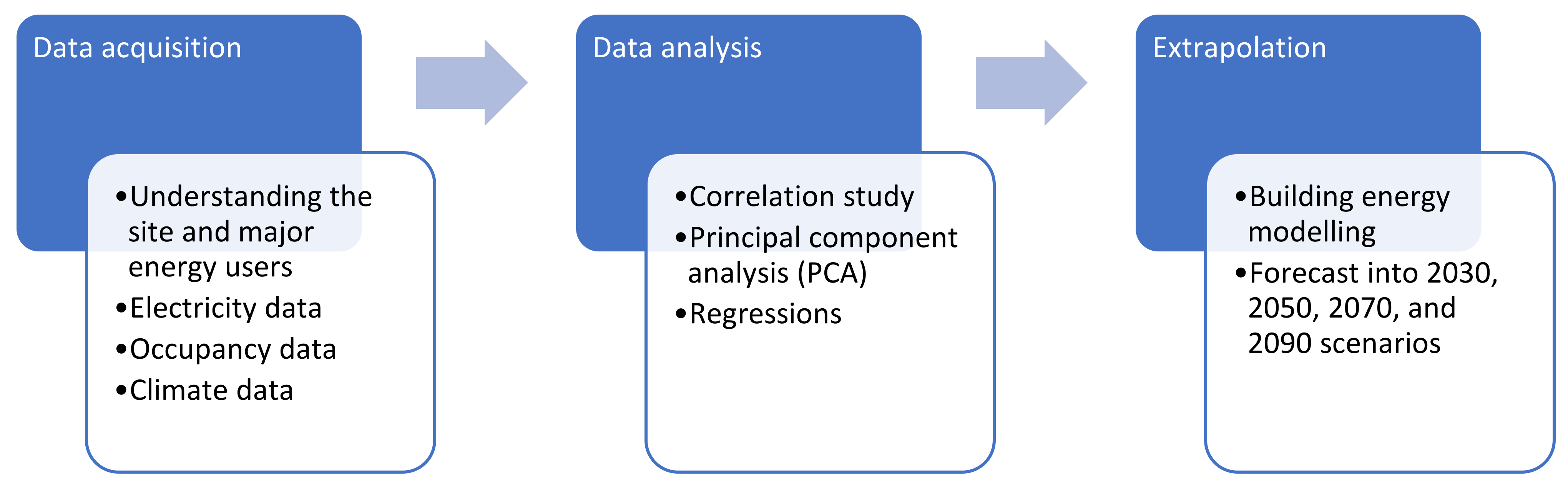
2. Inputs and Methods

The research methodology flow is illustrated in Figure 1. Overall, this research applies a suite of data analysis methods to a major modern hospital in subtropical Brisbane, Queensland, Australia [19].

2.1. Data Acquisition

At the data acquisition step, the site building types, operation mode, and major energy users were identified. In this research, the defined period is each calendar month because, in the Australian context, metering and billing are applied monthly for commercial and industrial (C&I) customers.
Monthly electricity use data and occupancy data can be obtained from site facility management. Occupancy data included occupied bed days and separations in each month. Occupied bed days are “the total number of bed days of all admitted patients” in a defined period [20]. Separations are the total number of patients who are recorded as having “cessation of treatment and/or care and/or accommodation” in a defined period [20].
Climate data can be obtained from a local Australian Bureau of Meteorology weather station (Table 1). Monthly climate data were used, and daily maximum and minimum temperatures were obtained from an Australian Bureau of Meteorology station, No. 040842 [21].

2.2. Data Analysis

After the site was understood and relevant data were obtained in the previous stage, this stage analysed the relationship between monthly electricity use data and occupancy data, and between monthly electricity use data and temperature data.
Three common analytical methods were applied: Pearson correlation coefficient (PCC), principal component analysis (PCA), and regression [22]. PCC has low computational requirements and can time-efficiently provide an overview of correlations between many sets of variables. Equation (1) calculates PCC, which is a value between −1 and +1, as an indicator for the relationship between changes in variable A and changes in variable B [23,24]. PCC ρ A , B is obtained using covariance between variable A and variable B C O V A ,   B divided by the standard deviation of A σ A and the standard deviation of B σ B .
ρ A , B = C O V A , B σ A σ B
Principal component analysis (PCA) uses the singular value decomposition method to identify another set of numerical components which may have fewer dimensions than the input datasets [10,25]. In this way, a reduced number of inputs may be identified with a similar accuracy in energy modelling. Consequently, reduced model complexity and lower computational overheads may be achieved.
In the regression part, polynomial fitting and artificial neural networks (ANN) are applied to the datasets. The models’ accuracy comparisons are undertaken to select the most accurate model. First-order polynomial fitting Equation (2) and second-order polynomial fitting Equation (3) are used in this research. X are monthly input variables used as matrix forms in (2) and (3). Also in (2) and (3), α , β , δ , η , θ are fitted coefficients for the two polynomial equations.
1 st   order   polynomial :   E = α X + β
2 nd   order   polynomial :   E = δ X . 2 + η X + θ
A single hidden-layer feedforward ANN with N number of hidden neurons and activation function g is presented in Equation (4) [26]:
G N X t = i = 1 N β i g W i X t + b i     w i t h   t = 1 , ,   T
where W i is the input weight vector; β i is the output weight vector; b i is the bias term; g is the activation function; T is the number of samples. The activation function is a smooth bounded monotonic function, often a sigmoid [27]. A backpropagation method has been commonly used to train neural network models [28]. Cross-validation is useful in terms of identifying the optimal ANN model for a given set of input variables [29].
For model Equations (2)–(4), inputs can include different combinations of monthly variables, such as monthly temperature variables, monthly occupancy variables, and a combination of both. Daily temperature inputs (row 2 and 3 of Table 1) are calculated into monthly intervals as a type of input variable. The three different models and combinations of inputs are evaluated with root mean squared errors (RMSE) and mean absolute errors (MAE) [30]. The model with the highest accuracy is selected for the next stage.

2.3. Forecasting

The Commonwealth Scientific and Industrial Research Organisation (CSIRO), Australia’s national science agency, has released future weather files for Australian climates in 2030, 2050, 2070, and 2090 scenarios [31], as described in Table 2. The temperature variables from these files are then recalculated into various monthly inputs, which are inserted into the best model identified out of Equations (2)–(4) to forecast the site’s future electricity use.
For this data-driven research, the following facts and assumptions are included:
  • No significant expansion is considered for the site precinct. The case study is a modern major urban vertical hospital and the physical site boundary is limited.
  • Like-for-like replacements are considered for existing facility assets when they are out of service lifetime. Potentially new assets would have higher efficiency for the same output rating.
  • Increased energy use due to new clinical equipment is largely offset by energy efficiency improvements from other facility assets.
  • Indoor thermal comfort is maintained through the 2030 to 2090 scenarios. For example, HVAC systems fully meet the thermal conditioning and ventilation needs of the site buildings.
The next section provides a site description first, followed by data analysis and forecast results into 2030 to 2090 climate scenarios.

3. Case Study Results

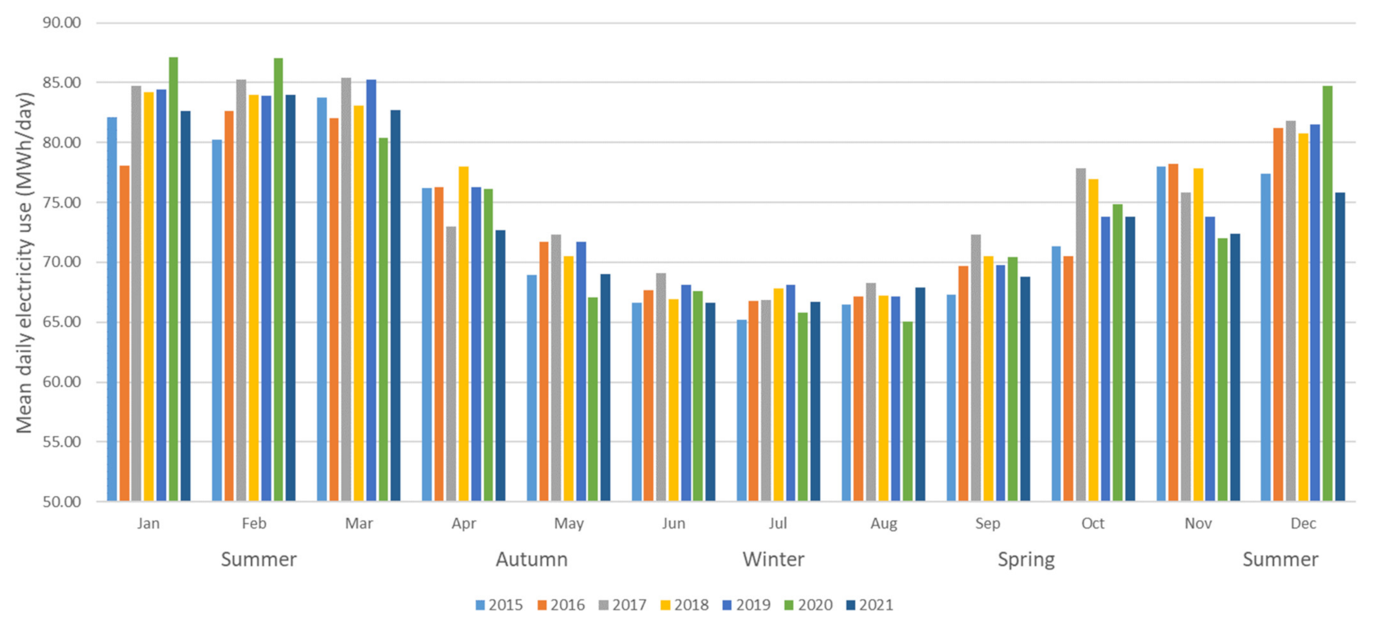
3.1. Case Study Site

The site is Queensland Children’s Hospital (QCH, coordinates: 27.4839° S 153.0279° E), a major modern hospital precinct commissioned in November 2014. The hospital precinct has three buildings with a total floor area of 134,800 m2. The site is in Australian Climate Zone 2, with warm humid summers and mild winters, and its Köppen Climate Classification is Cfa (Humid, Subtropical).
QCH is Queensland’s only quaternary hospital for children’s health and it accepts patients for the whole state of Queensland and northern New South Wales. QCH is also a COVID-19 hospital with negative pressure wards. Each year, QCH services an average of 100,000 occupied bed days and 40,000 separations (definitions in Section 2.1).
The QCH precinct uses a total of 26 to 27 GWh of electricity annually [19,34]. The HVAC system accounts for the largest share of electricity use onsite. Natural gas is used onsite to produce hot water (for domestic hot water and space heating) and steam, which will be studied in a future project and is beyond the scope of this article.
Exploratory data analysis indicates that the site energy is related to ambient temperature, as shown in Figure 2. Electricity use is regularly high in summer months from December to March, between 75 MWh/day and 87 MWh/day. Winter months from June to August tend to have lower electricity use, ranging between 65 MWh/day and 68 MWh/day. Mild months (April, May, September, October, November) are the ‘shoulder seasons’, transitioning between summer and winter.

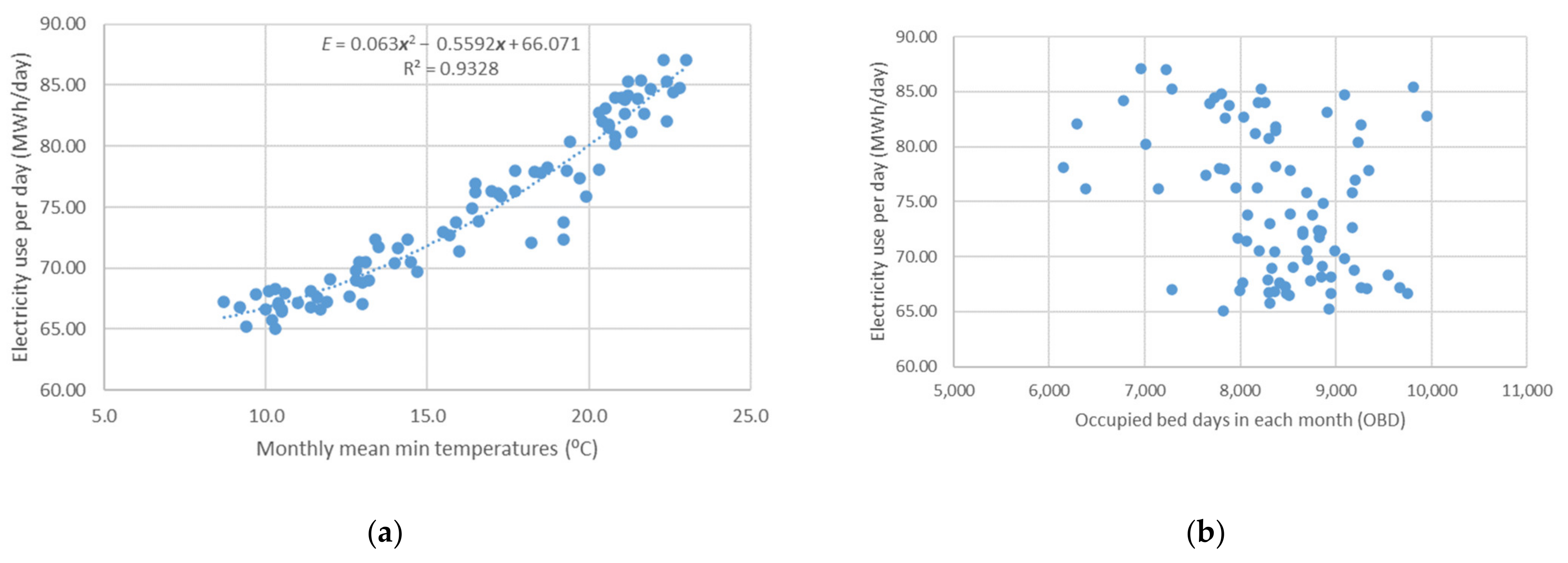
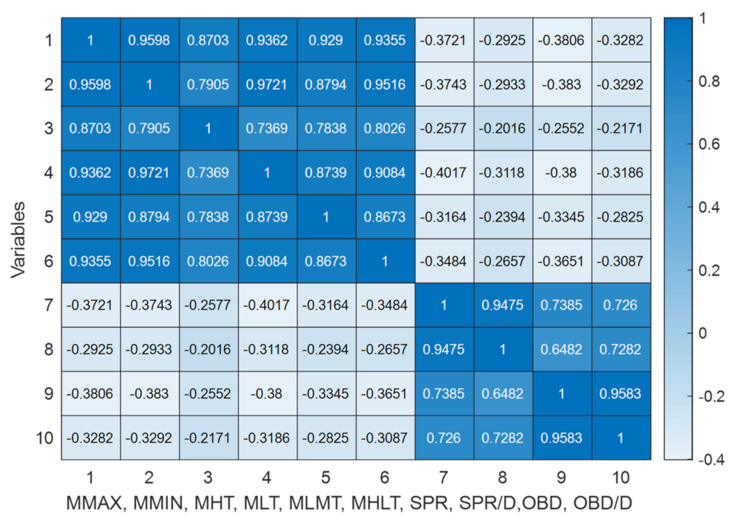
3.2. Correlation Study

Table 3 presents PCC values for monthly mean daily electricity use vs. six temperature variables, and monthly mean daily electricity use vs. four occupancy variables. Overall, monthly mean daily minimum temperatures have the highest PCC values with monthly mean daily electricity use. Regarding the temperature variables, monthly mean daily minimum temperatures and monthly lowest temperatures have the highest PCC values with monthly mean daily electricity use. No occupancy variable is highly correlated with the site energy use, while occupied bed days (OBD, row 9) and separations in each calendar month (row 7) have the highest PCC values among occupancy variables as inputs. All the PCC values can be considered statistically significant as all the p-values are less than 0.05 (if 0.95 is considered as the cut-off).
Then, the variables with the highest PCCs (row 2 and row 9 of Table 3) are plotted against the monthly mean daily electricity use values. Figure 3a presents the scatterplot for monthly mean daily electricity vs. monthly mean daily minimum temperature. A second-order fitting is also presented in the figure, with quite a good R2 value (goodness of fitting). However, there is no visible relationship shown between OBDs and the electricity use variable in Figure 3b.
Figure 4 shows cross-correlations calculated for the ten variables in Table 3. All the temperature variables are quite highly correlated, with PCC between 0.7389 and 0.9721, in the top left corner of Figure 4. Occupancy variables are mostly highly correlated with each other, with PCC between 0.6482 and 0.9583, in the bottom right corner of Figure 4. This indicates that for the site energy modelling, there is probably no need to have more than one variable out of those temperature variables, nor to have more than one variable from those occupancy variables. The next step, principal component analysis (PCA), helps to further determine key input variables, rather than having redundant variables of a similar nature.

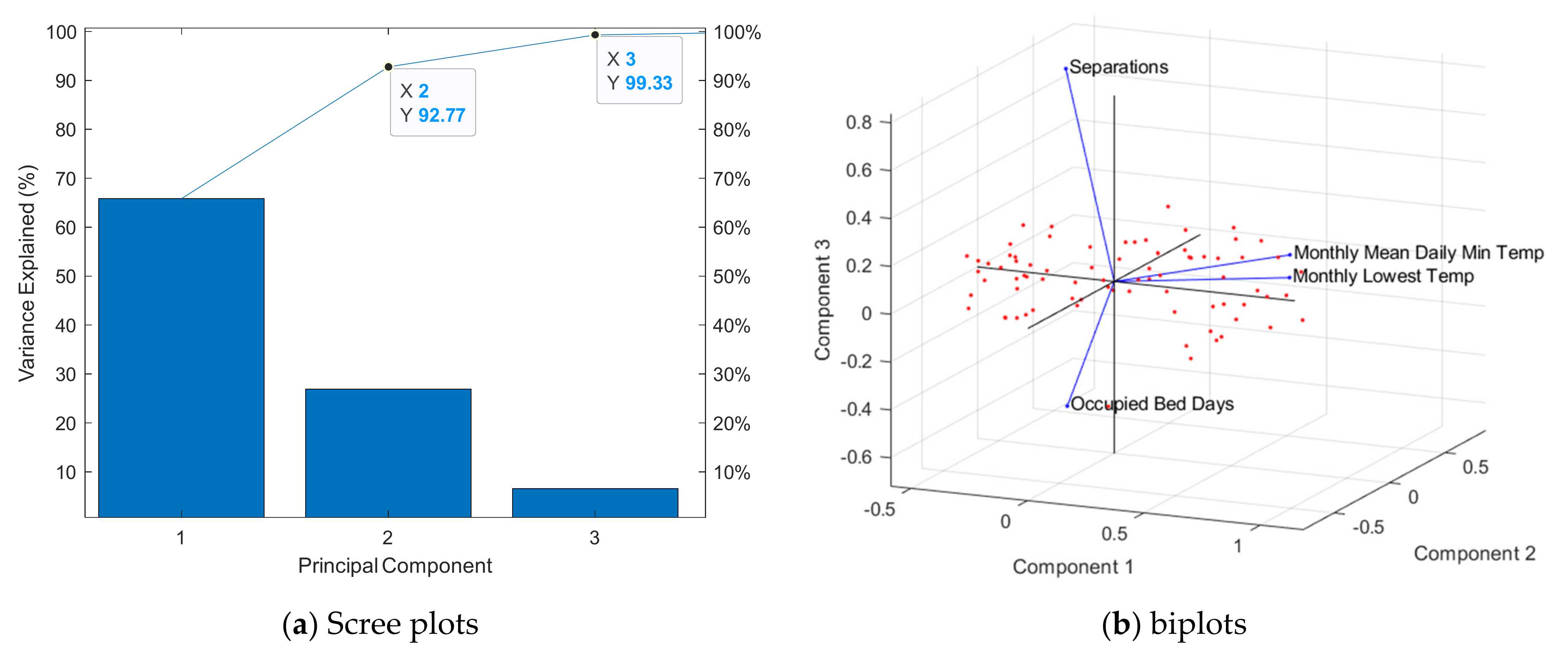
3.3. Principal Component Analysis

PCA can help to mathematically identify the principal components that are impactful for modelling and improve the multicollinearity issue. Two temperature variables and two occupancy variables were used in the principal component analysis, namely monthly mean daily minimum temperatures, monthly lowest temperatures, separations, and occupied bed days in each calendar month. The four variables were selected due to their leading PCC values in the previous analysis. PCA transforms input variables into another set of orthogonal principal components (PC).
Scree plots and analysis of PC can help to identify impactful PC and remove redundant variables. Figure 5a shows the scree plot of three principal components. The first principal component can explain 65.84% of variance; the first two PC together can explain 92.77% of variance, and the three PC together can explain 99.33% of variance.
Figure 5b shows the impacts of input variables on the three principal components. MDMIN and MLT are very close to each other and have similar impacts on the first PC. This indicates a need of having one of the two variables, rather than having both. SPR and OBD have similar impacts on the first PC and an opposite directional impact on the third PC. All four variables have similar impacts on the second PC.

3.4. Regressions

After the previous PCC and PCA analysis, monthly mean daily minimum temperatures (MMIN) were selected as the temperature input for the case study energy modelling. The occupancy modelling inputs can be either occupied bed days or separations.
Next, 2015 to 2020 data were used as the training datasets for model fitting and the latest 2021 data were used as the testing dataset to calculate the root mean squared error (RMSE) and mean absolute error (MAE) for the fitted models, as shown in Table 4. For the three types of fitting, both RMSE and MAE show that modelling with monthly mean minimum temperature inputs (MMIN) led to the best outcome because of the lowest RMSE and MAE values in each type of modelling, i.e., rows 1, 4, and 7. Modelling accuracy dropped when either occupied bed days (OBD) or separations (SPR) were added. The models with SPR tended to have higher accuracy than the models with OBDs.
Overall, ANN with monthly mean minimum temperature inputs (MMIN) on row 7 has the lowest RMSE, which is 23% better than row 4’s, and row 7’s MAE is also slightly better than row 4’s MAE. In the next section, ANN with MMIN inputs is used to forecast electricity use for the case study’s 2030 to 2090 scenarios.

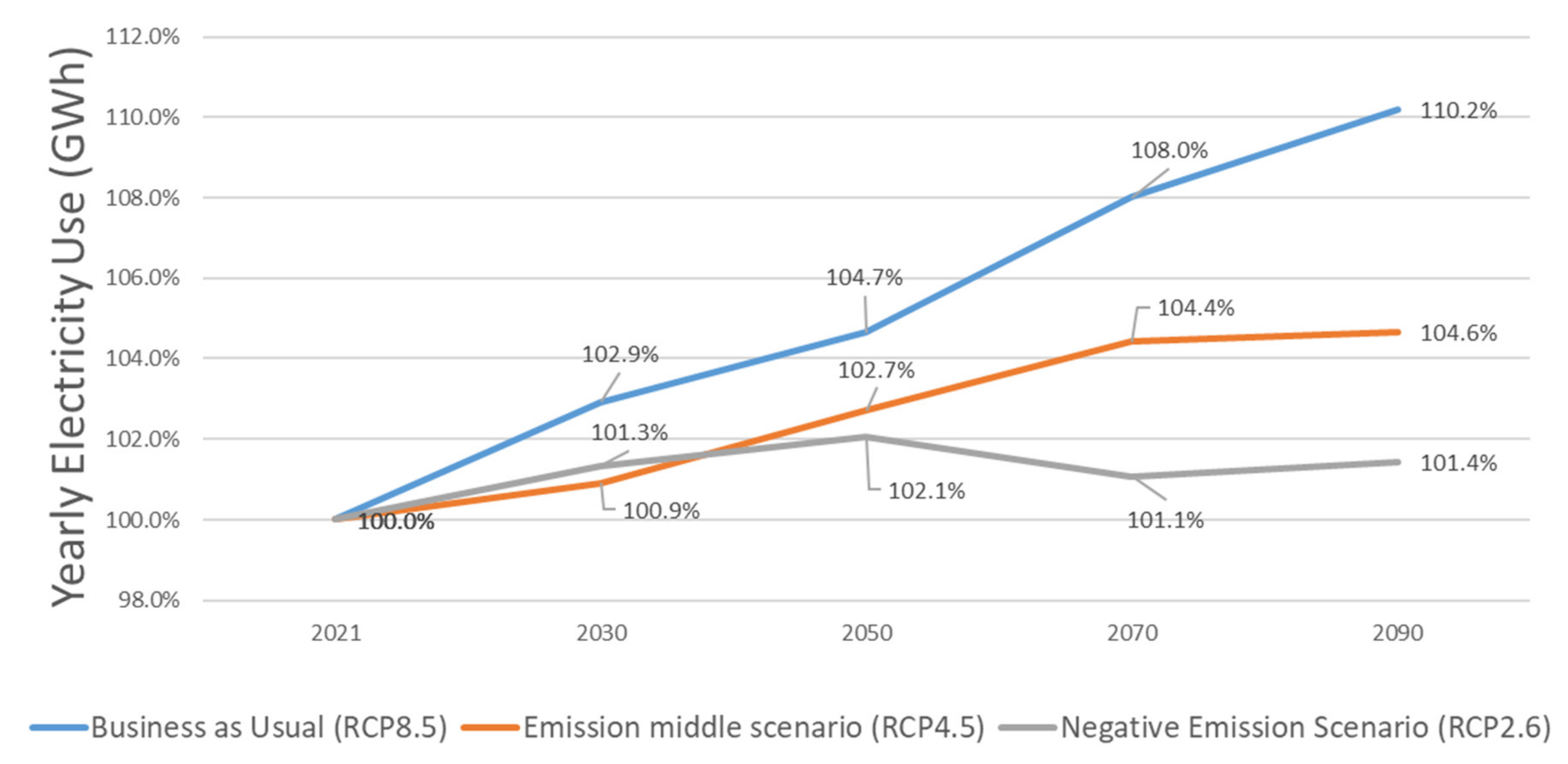
3.5. Forecast into 2030–2090 Scenarios

Figure 6 shows the case’s yearly electricity use forecast into 2030, 2050, 2070, and 2090 scenarios. In the business as usual (RCP8.5) scenario, more than 10% electricity use increase is forecast to happen by the period 2080 and 2100. In the best negative emission scenario (RCP2.6), the site’s yearly electricity use is predicted to have a mild increase of 1.4% by the end of the century. Data for the figure are provided in Table 5. These predictions are for typical yearly electricity use in each 20-year period. The potential financial and societal impacts are discussed in the next section.

4. Discussion

Across Australia, there are over 1300 public and private hospitals and 148 of these are major hospitals with over 100 beds [1,35]. QCH is one of the major hospitals. As the climate changes, there is a need to better understand the impact of the future climate on energy use, to better future-proof energy sustainability and financial sustainability for our healthcare sector. The following paragraphs discuss the implications of this research for operational expenditure, renewable energy, policy, and future developments.

4.1. Implication for Operational Expenditure

Assuming an electricity price of AUD 0.15/kWh in 2021 with a 2.5% per year cost increase [36,37,38], the site’s yearly electricity bill increases (above current baseline) for the 2030 to 2090 climate scenarios are presented in Table 6. The site’s electricity costs, a combination of increased energy use and increased cost per unit, places a very high financial burden on the hospital in the business as usual scenario (exceeding 1 million dollars for 2070 and 2 million dollars for 2090). On the positive side, the negative emissions scenario (RCP2.6 scenario) results in a much smaller cost increase. The public resource saving would be in the order of AUD 214,000 in 2050 and AUD 1,937,000 in 2090, if the RCP2.6 scenario occurs instead of RCP8.5. It is unclear whether any public health departments, already under financial pressure, have planned for the likelihood of significantly higher energy bills in the future.

4.2. Implication for Renewable Energy

Renewable energy has been a significant part of the public sector’s procurement strategy and it has been demonstrated to be effective in terms of carbon emission reductions [39]. Most Australian states and territories have set targets for achieving net zero carbon emissions and for increasing the share of renewable energy in the electricity sector. The outcome of this is demonstrated in the rising share of renewable energy as a share of national electricity, and the rising (but still small) share of public hospital energy use being met by renewables (Table 7, [39]).
Solar photovoltaic (PV) is one of the more common renewable technologies [40]. For this research, analysis was undertaken to determine the size of PV system (kWp) required to meet the increased electricity demand into the future. Table 8 shows that for the RCP8.5 and RCP4.5 scenarios, continuously increasing new PV capacity is needed to offset the site’s electricity use increase. Note that each future climate scenario is for a typical 20-year period, which is shorter than the expected life of PV panels (currently guaranteed performance over 25 to 30 years [14,41]). An implication of this is that new investments need to be put into place to construct new solar generation to meet the increased electricity use, as well as coping with declining efficiency for solar panels. It is also worth pointing out that this analysis only considers PVs to cover the increase in electricity demand, not the baseline use.

4.3. Implication for Policy and Future Developments

As the data analysis section shows, occupancy is not highly correlated with the site’s monthly energy use. There are a few potential reasons for why occupancy does not matter much for a major hospital in a warm climate:
  • For the case study, cooling is the dominant HVAC operation mode; electricity is the energy source for cooling. The major hospital is built with concrete and steel structures. Cooling to remove occupants’ metabolic load would probably be much less than the cooling needs for buildings’ thermal mass in the warm climate.
  • The HVAC settings in hospitals are typically determined by standards and regulations based on health, safety, and clinical reasons. The HVAC is typically centrally controlled, with little potential for patients and clinicians to change the thermostat settings. This particular hospital is air-conditioned 24-7 and uses 100% fresh air. This case study provides evidence from another angle to support [12]: occupancy may not be as significant as occupants’ behaviour in influencing energy use.
The consistent high correlation between electricity uses and temperature indicates a strong need to have a better building envelope for healthcare purposes, potentially through continuous improvement of health building guidelines [42]. Another related aspect is to have operational improvement for major space cooling-related equipment, such as optimising chillers’ staging and control [43]. Renovations between 2025 and 2090 may be great opportunities to improve the hospital building envelope and adopt energy efficiency technologies wherever technically feasible and financially viable.
A limitation of this study is that it was based on typical meteorological future climate files. The electricity use forecast results are for typical years within each 20-year period until the end of this century, rather than for years of extreme events, such as some years with extended periods of heatwaves. Higher levels of energy use increase would probably occur in future years, with increased intensity, magnitude, and duration of heatwaves as a result of climate change. This means that there is a need for the development of ‘extreme weather’ climate files that consider events such as extended periods of heatwaves. Such events are known to have an impact on energy, through increased utilisation of air conditioning, reduced efficiency of air conditioners and the electricity network, and increased risk of power failure [44]. Extreme weather climate files would enable modelling and simulation to understand the extent of the energy impacts and make decisions to avoid or limit the negative impacts [45].

5. Conclusions

This research has applied a suite of data analysis tools to model and forecast the energy use of a major modern hospital in subtropical Australia. Pearson correlation coefficients, principal component analysis, polynomial models, and artificial neural network models were used in the analysis and modelling process. With projected future weather files (2030, 2050, 2070, and 2090 scenarios), the hospital’s energy use was forecast to 2030 to 2090 with three RCP pathway scenarios, namely business as usual, a mid-emission scenario, and a negative emission scenario.
The data analysis results show that there is a low correlation between the case hospital’s occupancy and electricity use, but a high correlation with outdoor temperature. This highlights the need for a strong focus on improving the thermal efficiency of the building envelope (to minimise the growth in cooling load) as a priority.
Without addressing hospital buildings and HVAC systems, the changing climate is likely to significantly impact the hospital financially. For 2080–2100, the annual electricity bill could increase by more than AUD 2 million compared to 2021 in the business as usual scenario. This would impact the Queensland state budget, where public health regularly accounts for over 30% of the state’s budget [46]. Savings through hospital energy sustainability projects can offer an opportunity to alleviate some of the budgetary pressure.
This paper’s energy data analysis did not include energy for water heating, but water heating is a key factor of hospital energy use. Current Australian hospitals mostly use natural gas as the primary energy source to produce hot water or steam [47]. However, there are no data available for hot water use in this case study. A potential research direction is to analyse water heating energy use’s correlation with occupancy and explore scenarios of major hospitals with heating fully electrified.
It is likely that major modern hospitals in all climate zones of Australia will have cooling energy highly correlated with climate regardless of occupancy. Future work will test this inference and extend this analysis to include all states and territories of Australia (i.e., a range of climate zones). The outcomes of this data analysis approach to energy forecasting may also be compared with the outcomes of a building simulation approach. It is hoped to demonstrate that data analysis tools can be successfully used for this purpose in the absence of a building model, or in conjunction with a building simulation approach.

Author Contributions

Conceptualization, A.L. and W.M.; methodology, A.L.; software, A.L.; validation, A.L.; formal analysis, A.L., Y.M. and W.M.; investigation, A.L., W.M. and Y.M.; resources, W.M.; data curation, B.B.; writing—original draft preparation, A.L.; writing—review and editing, A.L., Y.M., W.M., B.X., B.B. and S.Z.; visualization, A.L.; supervision, W.M.; project administration, W.M. and B.B.; funding acquisition, W.M. All authors have read and agreed to the published version of the manuscript.

Funding

The research is part of an Australian Renewable Energy Agency Affordable Heating and Cooling Innovation Hub project (www.ihub.org.au (accessed on 3 March 2022)) funded by the Australian Government and Industry. Children’s Health Queensland Hospital and Health Services (Queensland Department of Health) has provided in-kind support for the case study site energy data acquisition.

Data Availability Statement

The climate dataset is publicly available on the Australian Bureau of Meteorology site: http://www.bom.gov.au/Climate (accessed on 3 March 2022). The raw data related to the site are proprietary. If there is an interest in collaboration, please contact the corresponding author.

Acknowledgments

The authors sincerely thank Children’s Health Queensland for the case study data and its effort in futureproofing healthcare environmental and financial resilience. Computational resources and services used in this work were provided by the Research Support Group, Queensland University of Technology (QUT), Brisbane, Australia.

Conflicts of Interest

The authors declare no conflict of interest. The funder, the Australian Renewable Energy Agency, had no role in the design of the study; in the collection, analysis, or interpretation of data; in the writing of the manuscript, or in the decision to publish the results.

Abbreviations

AcronymsDescription
PCCPearson Correlation Coefficient
PCAPrincipal Component Analysis
NNNeural Network
LRLinear Regression
CSIROThe Commonwealth Scientific and Industrial Research Organisation
OBDOccupied Bed Days in a Calendar Month
OBD/DOccupied Bed Days per Day in a Calendar Month
SPRSeparations in a Calendar Month
SPR/DSeparations per Day in a Calendar Month
MMAXMonthly Mean Daily Maximum Temperature
MMINMonthly Mean Daily Minimum Temperature
MHTMonthly Highest Temperature
MLTMonthly Lowest Temperature
MLMTMonthly Lowest Daily Maximum Temperature
MHLTMonthly Highest Daily Minimum Temperature
RCPRepresentative Concentration Pathway
SVDSingular Value Decomposition
RMSERoot Mean Squared Error

References

  1. Australian Institute of Health and Welfare Data Table: Hospital Resources 2018–2019. Available online: https://www.aihw.gov.au/reports-data/myhospitals/content/data-downloads (accessed on 9 May 2022).
  2. Xia, B.; E, J.; Chen, Q.; Buys, L.; Yigitcanlar, T.; Susilawati, C. Understanding Spatial Distribution of Retirement Villages: An Analysis of the Greater Brisbane Region. Urban Sci. 2021, 5, 89. [Google Scholar] [CrossRef]
  3. Miller, W.F.; Liu, A.; Crompton, G.; Ma, Y. Healthcare Sector Energy Baseline and Key Performance Indicators; Australian Institute of Refrigeration, Air-Conditioning and Heating (AIRAH): Brisbane, Australia, 2020. [Google Scholar]
  4. Building Energy Use in NSW Public Hospitals; New South Wales Government: Sydney, Australia, 2013.
  5. Karliner, J.; Slotterback, S.; Boyd, R.; Ashby, B.; Steele, K. Health Care’s Climate Footprint How the Health Sector Contributes to the Global Crisis and Opportunities for Action—Green Paper Number One; Health Care without Harm: Reston, VA, USA, 2019. [Google Scholar]
  6. Health Care Without Harm. Arup Australia Health Sector Emissions Fact Sheet; Health Care without Harm: Reston, VA, USA, 2018. [Google Scholar]
  7. Malik, A.; Lenzen, M.; McAlister, S.; McGain, F. The Carbon Footprint of Australian Health Care. Lancet Planet. Health 2018, 2, e27–e35. [Google Scholar] [CrossRef] [Green Version]
  8. Victorian Auditor-General’s Report Australia (Ed.) Energy Efficiency in the Health Sector; Victorian Government: Melbourne, Australia, 2012.
  9. Anand, P.; Deb, C.; Ke, Y.; Yang, J.; Cheong, D.; Sekhar, C. Occupancy-Based Energy Consumption Modelling Using Machine Learning Algorithms for Institutional Buildings. Energy Build. 2021, 252, 111478. [Google Scholar] [CrossRef]
  10. Zhan, S.; Chong, A. Building Occupancy and Energy Consumption: Case Studies across Building Types. Energy Built Environ. 2021, 2, 167–174. [Google Scholar] [CrossRef]
  11. Liu, A.; Miller, W.; Chiou, J.; Zedan, S.; Chen, X.; Susilawati, C. How Is Occupancy Related to Energy Use in Healthcare Buildings? In Proceedings of the 10th IEEE PES Innovative Smart Grid Technologies Conference—Asia, Brisbane, QLD, Australia, 5–8 December 2021; Saha, T.K., Ed.; IEEE: Brisbane, Australia, 2021. [Google Scholar]
  12. Ahn, K.-U.; Park, C.-S. Correlation between Occupants and Energy Consumption. Energy Build. 2016, 116, 420–433. [Google Scholar] [CrossRef]
  13. Wang, Y.; Chen, Q.; Hong, T.; Kang, C. Review of Smart Meter Data Analytics: Applications, Methodologies and Challenges. IEEE Trans. Smart Grid 2018, 10, 3125–3148. [Google Scholar] [CrossRef] [Green Version]
  14. Liu, A.; Miller, W.; Cholette, M.E.; Ledwich, G.; Crompton, G.; Li, Y. A Multi-Dimension Clustering-Based Method for Renewable Energy Investment Planning. Renew. Energy 2021, 172, 651–666. [Google Scholar] [CrossRef]
  15. Bawaneh, K.; Ghazi Nezami, F.; Rasheduzzaman, M.; Deken, B. Energy Consumption Analysis and Characterization of Healthcare Facilities in the United States. Energies 2019, 12, 3775. [Google Scholar] [CrossRef] [Green Version]
  16. Watts, N.; Adger, W.N.; Agnolucci, P.; Blackstock, J.; Byass, P.; Cai, W.; Chaytor, S.; Colbourn, T.; Collins, M.; Cooper, A.; et al. Health and Climate Change: Policy Responses to Protect Public Health. Lancet 2015, 386, 1861–1914. [Google Scholar] [CrossRef]
  17. Pencheon, D.; Rissel, C.E.; Hadfield, G.; Madden, D.L. Health Sector Leadership in Mitigating Climate Change: Experience from the UK and NSW. In New South Wales Public Health Bulletin; CSIRO: Sydney, Australia, 2009; Volume 20, pp. 173–176. [Google Scholar] [CrossRef] [Green Version]
  18. Nematchoua, M.K.; Yvon, A.; Kalameu, O.; Asadi, S.; Choudhary, R.; Reiter, S. Impact of Climate Change on Demands for Heating and Cooling Energy in Hospitals: An in-Depth Case Study of Six Islands Located in the Indian Ocean Region. Sustain. Cities Soc. 2019, 44, 629–645. [Google Scholar] [CrossRef]
  19. Liu, A.; Miller, W.F. Healthcare Living Laboratories: Queensland Children’s Hospital—Energy Baseline Data; Australian Institute of Refrigeration, Air-Conditioning and Heating (AIRAH): Brisbane, Australia, 2020. [Google Scholar]
  20. NABERS. Energy and Water for Hospitals: Rules for Collecting and Using Data; The National Australian Built Environment Rating System (NABERS): Sydney, Australia, 2017.
  21. Australian Bureau of Meterology Climate Data Online. Available online: http://www.bom.gov.au/climate/data/ (accessed on 15 June 2021).
  22. Trindade, F.C.L.; Ochoa, L.F.; Freitas, W. Data Analytics in Smart Distribution Networks: Applications and Challenges. In Proceedings of the 2016 IEEE Innovative Smart Grid Technologies—Asia (ISGT-Asia), Melbourne, Australia, 28 November–1 December 2016; pp. 574–579. [Google Scholar]
  23. Ma, Z.; Yan, R.; Nord, N. A Variation Focused Cluster Analysis Strategy to Identify Typical Daily Heating Load Profiles of Higher Education Buildings. Energy 2017, 134, 90–102. [Google Scholar] [CrossRef] [Green Version]
  24. Liu, A.L.; Shafiei, M.; Ledwich, G.; Miller, W.; Nourbakhsh, G.; Liu, L.; Shafiei, M.; Ledwich, G.; Miller, W.; Nourbakhsh, G. Correlation Study of Residential Community Demand with High PV Penetration. In Proceedings of the Australasian Universities Power Engineering Conference, Melbourne, Australia, 19–22 November 2017; Volume 2017, p. 6. [Google Scholar]
  25. Li, K.; Hu, C.; Liu, G.; Xue, W. Building’s Electricity Consumption Prediction Using Optimized Artificial Neural Networks and Principal Component Analysis. Energy Build. 2015, 108, 106–113. [Google Scholar] [CrossRef]
  26. Lolli, F.; Gamberini, R.; Regattieri, A.; Balugani, E.; Gatos, T.; Gucci, S. Single-Hidden Layer Neural Networks for Forecasting Intermittent Demand. Int. J. Prod. Econ. 2017, 183, 116–128. [Google Scholar] [CrossRef]
  27. Bennett, C.; Stewart, R.A.; Beal, C.D. ANN-Based Residential Water End-Use Demand Forecasting Model. Expert Syst. Appl. 2013, 40, 1014–1023. [Google Scholar] [CrossRef] [Green Version]
  28. Li, C.; Dong, Z.; Ding, L.; Petersen, H.; Qiu, Z.; Chen, G.; Prasad, D. Interpretable Memristive LSTM Network Design for Probabilistic Residential Load Forecasting. IEEE Trans. Circuits Syst. I Regul. Pap. 2022, 69, 1–14. [Google Scholar] [CrossRef]
  29. Yildiz, B.; Bilbao, J.I.; Dore, J.; Sproul, A.B. Recent Advances in the Analysis of Residential Electricity Consumption and Applications of Smart Meter Data. Appl. Energy 2017, 208, 402–427. [Google Scholar] [CrossRef]
  30. Hu, M.; Xiao, F.F.; Jørgensen, J.B.; Li, R. Price-Responsive Model Predictive Control of Floor Heating Systems for Demand Response Using Building Thermal Mass. Appl. Therm. Eng. 2019, 153, 316–329. [Google Scholar] [CrossRef]
  31. Ren, Z.; Tang, Z.; James, M. Projected Weather Files for Building Energy Modelling—User Guide; CSIRO: Canberra, Australia, 2022.
  32. IPCC. Climate Change 2014: Synthesis Report; Intergovernmental Panel on Climate Change (IPCC): Geneva, Switzerland, 2014. [Google Scholar]
  33. Foo, G. Climate Change: Impact on Building Design and Energy Final Report; DeltaQ: Canberra, Australia, 2020. [Google Scholar]
  34. Liu, A.; Miller, W.F. Healthcare Living Laboratories: Queensland Children’s Hospital—Operation Manual and Baseline Data; Queensland University of Technology: Brisbane, Australia, 2020. [Google Scholar]
  35. Australian Institute of Health and Welfare Australian Hospital Peer Groups Appendix C: Alphabetical Listing of Public and Private Hospitals by Peer Group 2019. Available online: https://www.aihw.gov.au/reports/hospitals/australian-hospital-peer-groups/data (accessed on 9 May 2022).
  36. Reserve Bank of Australia. Australia’s Inflation Target; Reserve Bank of Australia: Sydney, Australia, 2017.
  37. Ma, Y.; Saha, S.C.; Miller, W.; Guan, L. Parametric Analysis of Design Parameter Effects on the Performance of a Solar Desiccant Evaporative Cooling System in Brisbane, Australia. Energies 2017, 10, 849. [Google Scholar] [CrossRef] [Green Version]
  38. Liu, A.; Miller, W. Healthcare Living Laboratories: Queensland Children’s Hospital—Exergenics QCH Chiller System Digital Twin and Optimisation; Australian Institute of Refrigeration, Air-Conditioning and Heating (AIRAH): Brisbane, Australia, 2021. [Google Scholar]
  39. Burch, H.; Anstey, M.H.; McGain, F. Renewable Energy Use in Australian Public Hospitals. Med. J. Aust. 2021, 215, 160–163. [Google Scholar] [CrossRef]
  40. Cortese, T.T.P.; Almeida, J.F.S.D.; Batista, G.Q.; Storopoli, J.E.; Liu, A.; Yigitcanlar, T. Understanding Sustainable Energy in the Context of Smart Cities: A PRISMA Review. Energies 2022, 15, 2382. [Google Scholar] [CrossRef]
  41. Chen, X.; Qu, K.; Calautit, J.; Ekambaram, A.; Lu, W.; Fox, C.; Gan, G.; Riffat, S. Multi-Criteria Assessment Approach for a Residential Building Retrofit in Norway. Energy Build. 2020, 215, 109668. [Google Scholar] [CrossRef]
  42. Guidelines for Sustainability in Capital Works—Creating Healthier Resilient Buildings for a Changing Climate; Victoria State Government: Melbourne, Australia, 2020.
  43. Liu, A.; Miller, W. Healthcare Living Laboratories: Queensland Children ’s Hospital: Technology Evaluation Report for Exergenics’ Optimised Chiller Staging; Queensland University of Technology: Brisbane, Australia, 2022. [Google Scholar]
  44. Panteli, M.; Mancarella, P. Influence of Extreme Weather and Climate Change on the Resilience of Power Systems: Impacts and Possible Mitigation Strategies. Electr. Power Syst. Res. 2015, 127, 259–270. [Google Scholar] [CrossRef]
  45. Moazami, A.; Nik, V.M.; Carlucci, S.; Geving, S. Impacts of Future Weather Data Typology on Building Energy Performance—Investigating Long-Term Patterns of Climate Change and Extreme Weather Conditions. Appl. Energy 2019, 238, 696–720. [Google Scholar] [CrossRef]
  46. Queensland Government. Queensland State Budget 2021–2022. Available online: https://www.treasury.qld.gov.au/resource/state-budget-2021-22/ (accessed on 1 February 2022).
  47. Evans, M.; Belusko, M.; Taghipour, A.; Liu, M.; Keane, P.F.; Nihill, J.; Amin, R.; Liu, A.; Assaf, J.; Lau, T.; et al. RACE for 2030 CRC Research Theme B3 Electrification & Renewables to Displace Fossil Fuel Process Heating Opportunity Assessment Final Report; University of South Australia: Adelaide, Australia, 2021. [Google Scholar]
Figure 1. Research flowchart.
Buildings 12 01116 g001
Figure 2. Monthly mean daily electricity use (MWh/day).
Buildings 12 01116 g002
Figure 3. Scatterplots: (a) monthly mean daily minimum temperature vs. monthly electricity use per day; (b) monthly occupied bed days vs. monthly electricity use per day.
Buildings 12 01116 g003
Figure 4. Cross-correlations of potential input variables.
Buildings 12 01116 g004
Figure 5. PCA plots: (a) scree plots to show principal components for percentages of variance explained; (b) biplots to show impacts of input variables on principal components.
Buildings 12 01116 g005
Figure 6. Benchmarking of electricity forecast into 2030–2090 scenarios.
Buildings 12 01116 g006
Table 1. Data types and description.
No.DescriptionUnits
1Monthly electricity useKilowatt-hours (kWh)
2Daily maximum temperaturesDegree Celsius (°C)
3Daily minimum temperaturesDegree Celsius (°C)
4Monthly separationsSeparations (SPR)
5Monthly occupied bed daysOccupied bed days (OBD)
Table 2. Australian future climate scenarios.
Future Scenario NamesDescriptionPathways
2030representing a typical year between 2020 and 2040
  • Business as usual pathway, Representative Concentration Pathway 8.5 (RCP8.5) [32]
  • Emission middle pathway (RCP4.5)
  • Negative emission pathway (RCP2.6). RCP2.6 is the only pathway to maintain the average temperature increase <1.5 °C [33].
2050representing a typical year between 2040 and 2060
2070representing a typical year between 2060 and 2080
2090representing a typical year between 2080 and 2100
Table 3. Pearson correlation coefficients.
No.TypesMonthly Mean Daily Electricity Use vs. PCCp-Values
1Temperature variablesMonthly mean daily maximum temperatures (MMAX)0.9325.320 × 10−38
2Monthly mean daily minimum temperatures (MMIN)0.9561.626 × 10−45
3Monthly highest temperatures (MHT)0.7755.397 × 10−18
4Monthly lowest temperatures (MLT)0.9382.317 × 10−39
5Monthly lowest daily maximum temperature (MLMT)0.8492.113 × 10−24
6Monthly highest daily minimum temperature (MHLT)0.9221.423 × 10−35
7Occupancy variablesSeparations in each calendar month (SPR)−0.3000.006
8Separations per day in each calendar month (SPR/D)−0.2240.041
9Occupied bed days in each calendar month (OBD)−0.3310.002
10OBD per day in each calendar month (OBD/D)−0.2790.010
Table 4. Model accuracy comparisons.
No.Description RMSEMAE
11st order polynomial with MMIN 2.66391.9587
21st order polynomial with MMIN and OBD2.86701.9970
31st order polynomial with MMIN and SPR2.70791.9611
42nd order polynomial with MMIN 2.36181.4807
52nd order polynomial with MMIN and OBD2.62991.7080
62nd order polynomial with MMIN and SPR2.39741.5322
7ANN with MMIN (10 neurons)1.80931.4593
8ANN with MMIN and OBD (15 neurons)2.32341.8113
9ANN with MMIN and SPR (11 neurons)2.03461.5951
Table 5. Electricity use forecast into future climate scenarios.
Climate Scenario NamesDescriptionEmission Business as Usual
(RCP8.5)
Emission Middle Scenario
(RCP 4.5)
Emission Negative Scenario
(RCP2.6)
2021Yearly electricity use (GWh)26.846 (base)
2030Typical yearly use between 2020 and 2040 (GWh)27.63227.08927.206
Increase compared to 20212.9%0.9%1.3%
2050Typical yearly use between 2040 and 2060 (GWh)28.09427.57227.397
Increase compared to 20214.7%2.7%2.1%
2070Typical yearly use between 2060 and 2080 (GWh)28.99528.03327.133
Increase compared to 20218.0%4.4%1.1%
2090Typical yearly use between 2080 and 2100 (GWh)29.57928.09327.230
Increase compared to 202110.2%4.6%1.4%
Table 6. Yearly bill increase in future climate scenarios.
Climate
Scenarios
Business as Usual (RCP8.5) a,bEmission Middle
Scenario (RCP4.5) a,b
Negative Emission Scenario (RCP2.6) a,bSavings Comparing RCP2.6 to RCP8.5
2030$147,255$45,602$67,501$79,754
2050$383,318$223,028$169,246$214,073
2070$1,081,181$597,236$144,658$936,523
2090$2,253,117$1,027,949$316,407$1,936,710
Notes: a Electricity is assumed to be AUD 0.15/kWh in 2021 excluding goods and services tax. b Electricity price is considered to increase 2.5% annually, in line with Australia’s official long-term inflation target [36].
Table 7. Renewable energy baselines and percentages.
Energy2016/172017/182018/19
National baseline renewables15.7%17.0%24.0%
Total hospital energy consumed4,132,162 MWh4,213,694 MWh4,121,911 MWh
Hospital renewable energy produced13,651 MWh18,350 MWh94,415 MWh
Hospital energy % renewable0.33%0.44%2.29%
Table 8. New solar capacity to offset the increased electricity use compared to 2021 (kW peak).
Climate
Scenarios
Business as Usual (RCP8.5) aEmission Middle Scenario (RCP4.5) aNegative Emission Scenario (RCP2.6) a
2030513159235
2050815474360
20701402775188
20901783814250
Note: a 1 kW peak solar photovoltaic systems in this region generate a yearly average of 4.2 kWh/day.
Publisher’s Note: MDPI stays neutral with regard to jurisdictional claims in published maps and institutional affiliations.

