A Grasshopper Optimization Algorithm-Based Response Surface Method for Non-Probabilistic Structural Reliability Analysis with an Implicit Performance Function

Abstract

Non-probabilistic reliability analysis has great developmental potential in the field of structural reliability analysis, as it is often difficult to obtain enough samples to construct an accurate probability distribution function of random variables based on probabilistic theory. In practical engineering cases, the performance function (PF) is commonly implicit. Monte Carlo simulation (MCS) is commonly used for structural reliability analysis with implicit PFs. However, MCS requires the calculation of thousands of PF values. Such calculation could be time-consuming when the structural systems are complicated, and numerical analysis procedures such as the finite element method have to be adopted to obtain the PF values. To address this issue, this paper presents a grasshopper optimization algorithm-based response surface method (RSM). First, the method employs a quadratic polynomial to approximate the implicit PF with a small set of the actual values of the implicit PF. Second, the grasshopper optimization algorithm (GOA) is used to search for the global optimal solution of the scaling factor of the convex set since the problem of solving the reliability index is transformed into an unconstrained optimal problem. During the search process in the GOA, a dynamic response surface updating strategy is used to improve the approximate accuracy near the current optimal point to improve the computing efficiency. Two mathematical examples and two engineering structure examples that use the proposed method are given to verify its feasibility. The results compare favorably with those of MCS. The proposed method can be non-invasively combined with finite element analysis software to solve non-probabilistic reliability analysis problems of structures with implicit PF with high efficiency and high accuracy.

1. Introduction

To address the uncertain factors in a structure, it is necessary to reasonably select a mathematical model that quantifies the uncertain factors and structural reliability. Many analytical- and simulation-based methods have been developed to calculate the failure probability and reliability index of structures [1,2]. Among them, Monte Carlo simulation (MCS) is probably the most widely used high-precision structural reliability analysis method. However, when the probability of structural failure is small, MCS often needs to simulate a large number of samples to obtain accurate probability values, which will increase a lot of computational costs. Some improved methods, such as the subset simulation method [3], the line sampling method [4], and the importance sampling method (IS) [5], still have a high computation when facing complex problems. Analytical methods, such as first-order reliability methods (FORMs) and second-order reliability methods (SORMs), are computationally efficient but are often not stable enough in the face of structures with implicit PFs. For some improved algorithms, such as the directional stability transformation method (DSTM) [6] and finite-step adaptive length (FAL) [7], it is difficult to solve the convex set reliability problem [8]. On the other hand, by the type of random variable in the structures, Cremona [9] divided structural reliability models into random reliability models, fuzzy reliability models, non-probabilistic reliability models, and mixtures of the three models according to the mechanism of uncertainty factors. Among the various uncertainty models, the most widely used is the probabilistic reliability model based on probability theory and stochastic processes [10,11,12]. However, it is difficult to obtain sufficient statistical sample data in practical engineering structures to construct the probability distribution function of a probabilistic model. Additionally, a small fitting error of the probability distribution function of a random reliability model can lead to a large structural reliability calculation error [13]. This is especially true when there are few samples with which the model can calculate [14].

To address the condition of insufficient samples, in 1993, Ben-Haim [15] and Elishakoff [16] proposed a non-probabilistic reliability model for structural analysis and applied the maximum uncertainty allowed in the system to evaluate the structural reliability. Non-probabilistic reliability theory uses an artificially defined set model to describe the uncertain variables of the structure. The non-probabilistic reliability model only needs the range of the uncertain variables and then constructs the mapping relationship between the uncertain variables and the corresponding feasible domain of the structure under the combined action of multiple variables. It can be seen from this that it is particularly important to use the non-probabilistic reliability method in the reliability analysis of complex engineering structures. Due to factors such as safety and cost, it is difficult to carry out enough field experiments to obtain enough actual samples to establish reliable probability distribution functions in complex engineering structures [17]. Furthermore, small deviations in the probability density function due to data noise are likely to lead to large result errors [13]. However, in the same situation, using a small number of field experiments, the range of random variables can be quickly obtained, and then a structural reliability analysis with high reliability can be constructed through the non-probabilistic reliability method. Then, by comparing the set model and the limit state surface defined by the performance function (PF), the structural reliability index can be evaluated. Subsequently, scholars have conducted many studies that can be summarized into two categories: proposing different non-probabilistic reliability models aimed at better describing multivariable problems and studying how to quantify non-probabilistic reliability indicators according to different models. In 1998, Qiu and Elishakoff [18] used interval theory to establish an interval model to optimize a six-bar truss. In 2011, Wang et al. [19,20] proposed a non-probabilistic reliability model measurement index based on an interval model, where the index was defined by the ratio of the volume of the safety domain of the structure to the total volume of the basic interval variable domain. The interval model can only deal with independent variables [21]; therefore, scholars further proposed ellipsoid models to deal with dependent variables. In 1998, Pantelides et al. [22] proposed an ellipsoid model and compared the structural analysis results of different working conditions based on the ellipsoid model. In 2011, Jiang et al. [23] proposed a modeling method to establish a multidimensional ellipsoid model. To make the dependence of uncertain variables explicit, they introduced a covariance matrix to evaluate the correlations of dependent variables. In 2016, Kang and Zhang [24] constructed a mathematical formula system to develop a compact ellipsoid model. Recently, to address the problem of including independent and dependent variables, scholars have proposed more general models. In 2015, Jiang et al. [21] proposed a multidimensional parallelepiped model that can efficiently deal with complex ‘multi-source uncertainty’ problems. Guo et al. [25] proposed a mixed model composed of a hypercube interval model and a hyper-ellipsoid model. In 2021, Cao et al. [26] proposed a quantifying strategy for non-probabilistic uncertainties by combining the general polygonal convex set model and cluster polygonal convex set model. However, with the development of non-probabilistic reliability models and quantitative indices of reliability, solving non-probabilistic reliability problems quickly and accurately has become a restriction on related field development.

To address the above problems, scholars have explored many methods. Jiang et al. [23] applied the first-order reliability method (FORM) to a non-probabilistic convex model based on multidimensional ellipsoids for uncertainty. Wang et al. [27] proposed an improved second-order reliability method (SORM) for reliability analysis in the presence of both random and interval variables. These methods perform well in reliability analysis with explicit PFs; however, in practical engineering cases, the PF is commonly implicit. Therefore, it is difficult to obtain the exact boundaries of the structural failure domain and the reliable domain. For more complex structures, the reliability can only be calculated by numerical simulation methods such as finite element analysis (FEA), which are very time-consuming in most practical engineering applications. Therefore, the use of an explicit surrogate model of PFs for structural reliability analysis has become mainstream. One of the most commonly used methods is the response surface method (RSM). In 1989, Faravelli [28] first proposed a quadratic polynomial regression model to approximate a function, and this method is also called the classical RSM. The response surface can quickly and accurately fit an implicit PF and, at the same time, can eliminate the interference caused by sample noise through probabilistic methods. RSMs can be simply divided into two types: regression-based models and interpolation-based models [29]. Regression-based models, such as Gaussian process regression [12,30,31], use the probabilistic properties of known samples to perform regression analysis to fit functions in the feasible domain. An alternative model is based on general polynomial chaos expansion (gPCE) [32,33,34]. In this surrogate model, the random variables are placed in the random space expanded by orthogonal polynomials. The coefficients of each dimension are multiplied by the corresponding orthogonal polynomials, and then added to obtain the explicit surrogate model of the implicit PF. Interpolation-based models, such as support vector machines [35,36] and artificial neural networks [37,38,39], correct the values of the weight parameters of the model by learning the characteristics of the known samples to interpolate the function in the feasible domain. However, the RSMs mentioned above are all aimed at probabilistic reliability, and research on RSMs aimed at non-probabilistic reliability is still very rare.

This paper proposes a grasshopper optimization algorithm (GOA)-based RSM for the non-probabilistic reliability analysis of structures with implicit PFs. In this method, a quadratic polynomial response surface is presented to fit the PF. Notably, for general engineering structures, although the newly proposed RSM has high accuracy, the fitting speed is slow. Additionally, the hyper-parameters in models such as support vector machine (SVM) are difficult to determine without manual parameter adjustment [40]. In contrast, the application of the quadratic polynomial RSM in the field of probabilistic reliability is very mature [41] and can be quickly fitted while largely guaranteeing the fitting accuracy in general structures. Then, the proposed method uses a dynamic fitting strategy to find the approximate location of the generalized design point and then performs local fitting of the PF around the generalized design point. To find the globally optimal solution faster in the process of calculating the non-probabilistic reliability index, the GOA is used to search for the reliability index and optimal design point of the structure. This paper is organized as follows: Section 2 introduces the convex model theory to quantify the non-probabilistic reliability with the reliability index. 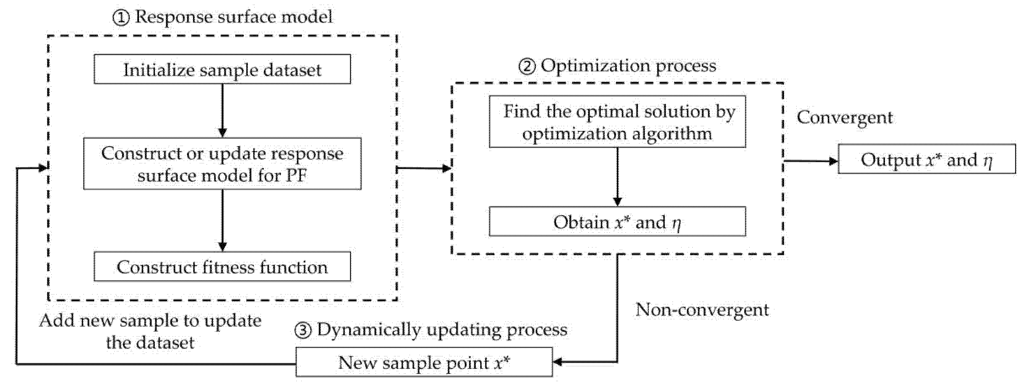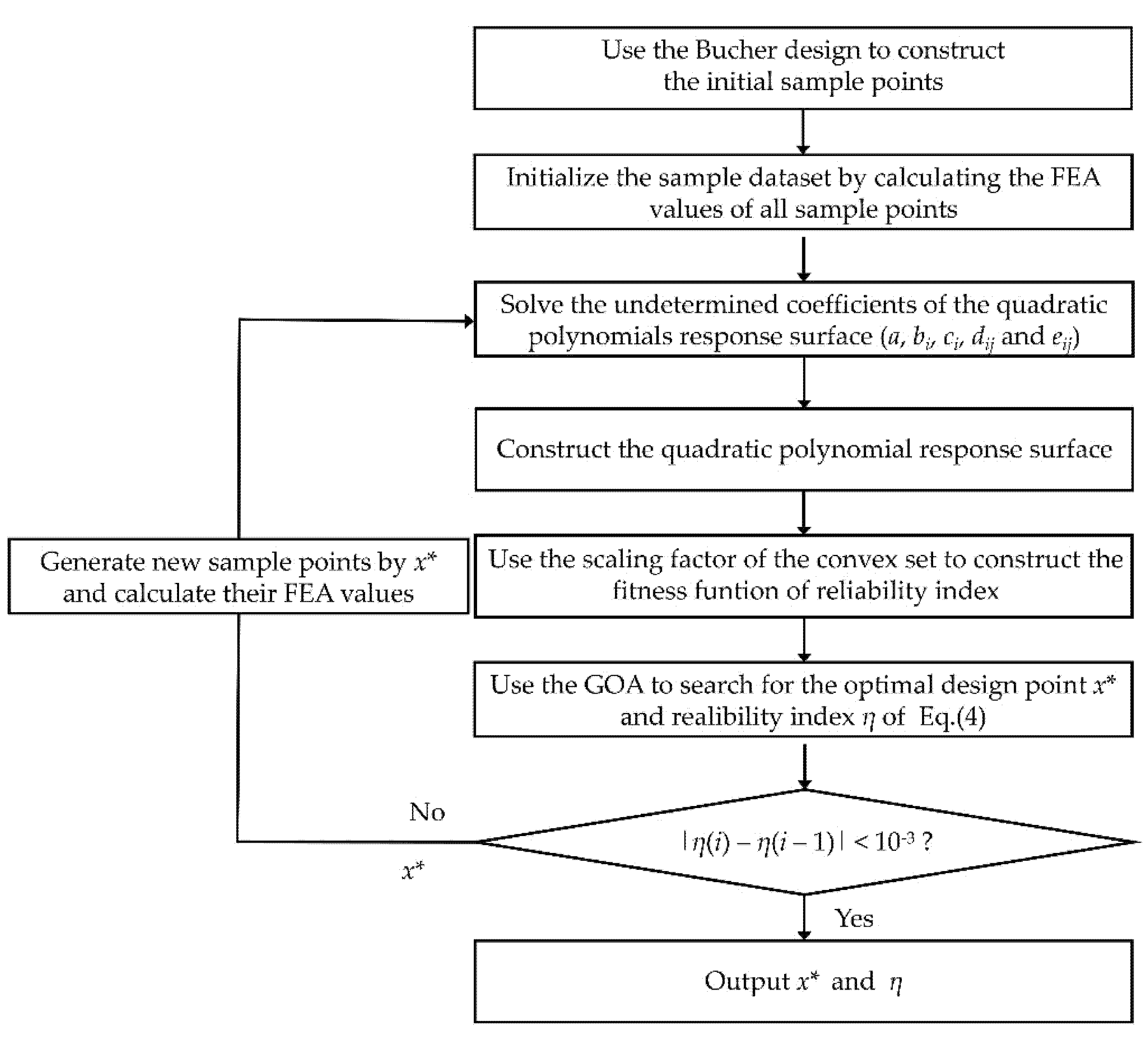Section 3 presents the framework of the proposed method. According to the framework, Section 4 introduces the key technologies of the proposed method. Section 5 introduces the detailed implementation of the proposed method based on the key technologies. Section 6 gives four examples—two mathematical examples and two engineering structure examples—to verify the feasibility of the proposed method. Finally, Section 7 summarizes the conclusion for the proposed method according to the examples.

2. Reliability Index of Non-Probabilistic Reliability

A non-probabilistic reliability model is an effective way to deal with structures with insufficient samples. The question arises of how to characterize the safety of structures in a non-probabilistic setting. Many scholars have proposed multiple reliability indices to quantify the non-probabilistic reliability [42,43,44]. The use of a scaling factor for convex sets is one of the most common methods.

According to the properties of the convex model, the total uncertainty of a structure is the intersection set of m convex sets of all uncertainties [37]. This intersection set can also be considered a feasible domain for the structure to remain stable under the impact of multiple uncertain variables. It can be represented as:

$$\mathit{X}(\mathit{\alpha },\hspace{0.33em}\overline{\mathit{X}})=\underset{i=1}{\overset{n}{\cap }}{\mathit{X}}_i=\left\{\begin{array}{c}\mathit{X}=({\mathit{x}}_1,\hspace{0.33em}\dots ,\hspace{0.33em}{\mathit{x}}_n):{\mathit{x}}_i\in {\mathit{X}}_j({\mathit{\alpha }}_i,\hspace{0.33em}{\overline{\mathit{x}}}_i),\hspace{0.33em}j=1,\hspace{0.33em}\dots ,\hspace{0.33em}m,\\ {\mathit{X}}_1=({\mathit{x}}_1,\hspace{0.33em}\dots ,\hspace{0.33em}{\mathit{x}}_{n_1}),\hspace{0.33em}\dots ,\hspace{0.33em}{\mathit{X}}_m=({\mathit{x}}_{n_{m-1}+1},\hspace{0.33em}\dots ,\hspace{0.33em}{\mathit{x}}_{n_m}),\hspace{0.33em}n=n_m\end{array}\right\}$$

(1)

where $\mathit{\alpha }=\{{\mathit{\alpha }}_1,\hspace{0.33em}{\mathit{\alpha }}_2,\hspace{0.33em}\dots ,\hspace{0.33em}{\mathit{\alpha }}_n\}$ is the size parameter of the convex set family of total uncertain variables, $\overline{\mathit{X}}=\{{\overline{\mathit{x}}}_1,\hspace{0.33em}{\overline{\mathit{x}}}_2,\hspace{0.33em}\dots ,\hspace{0.33em}{\overline{\mathit{x}}}_n\}$ is the position parameter of the convex set family of total uncertain variables, and ${\mathit{X}}_m=({\mathit{x}}_{n_{m-1}+1},\dots ,{\mathit{x}}_{n_m})$ represents a subset of uncertain variables with the same convex set. The stability of the structure under a certain working condition can be determined by Equation (1).

The scale factor $\lambda$ can be used to freely scale the intersection set in Equation (1). The scaled intersection set is as follows:

$$\mathit{X}(\lambda ,\mathit{\alpha },\hspace{0.33em}\overline{\mathit{X}})=\underset{i=1}{\overset{n}{\cap }}{\mathit{X}}_i=\left\{\begin{array}{l}\mathit{X}=({\mathit{x}}_1,\hspace{0.33em}\dots ,\hspace{0.33em}{\mathit{x}}_n):{\mathit{x}}_i\in {\mathit{X}}_j({\lambda \mathit{\alpha }}_i,\hspace{0.33em}{\overline{\mathit{x}}}_i),\hspace{0.33em}j=1,\hspace{0.33em}\dots ,\hspace{0.33em}m,\hfill \\ {\mathit{X}}_1=({\mathit{x}}_1,\hspace{0.33em}\dots ,\hspace{0.33em}{\mathit{x}}_{n_1}),\hspace{0.33em}\dots ,\hspace{0.33em}{\mathit{X}}_m=({\mathit{x}}_{n_{m-1}+1},\hspace{0.33em}\dots ,\hspace{0.33em}{\mathit{x}}_{n_m}),\hspace{0.33em}n=n_m\hfill \end{array}\right\}$$

(2)

The factor acts on the size parameter of each convex set. When the above intersection set in Equation (2) is increased by the factor $\lambda$ to intersect the failure domain divided by the PF, this indicates that the structure is in a failure state under some combination of uncertain variables. Therefore, $\lambda$ must be reduced until the intersection is tangent to the failure domain. This tangent point represents the generalized design point of the structure on the PF [45]. 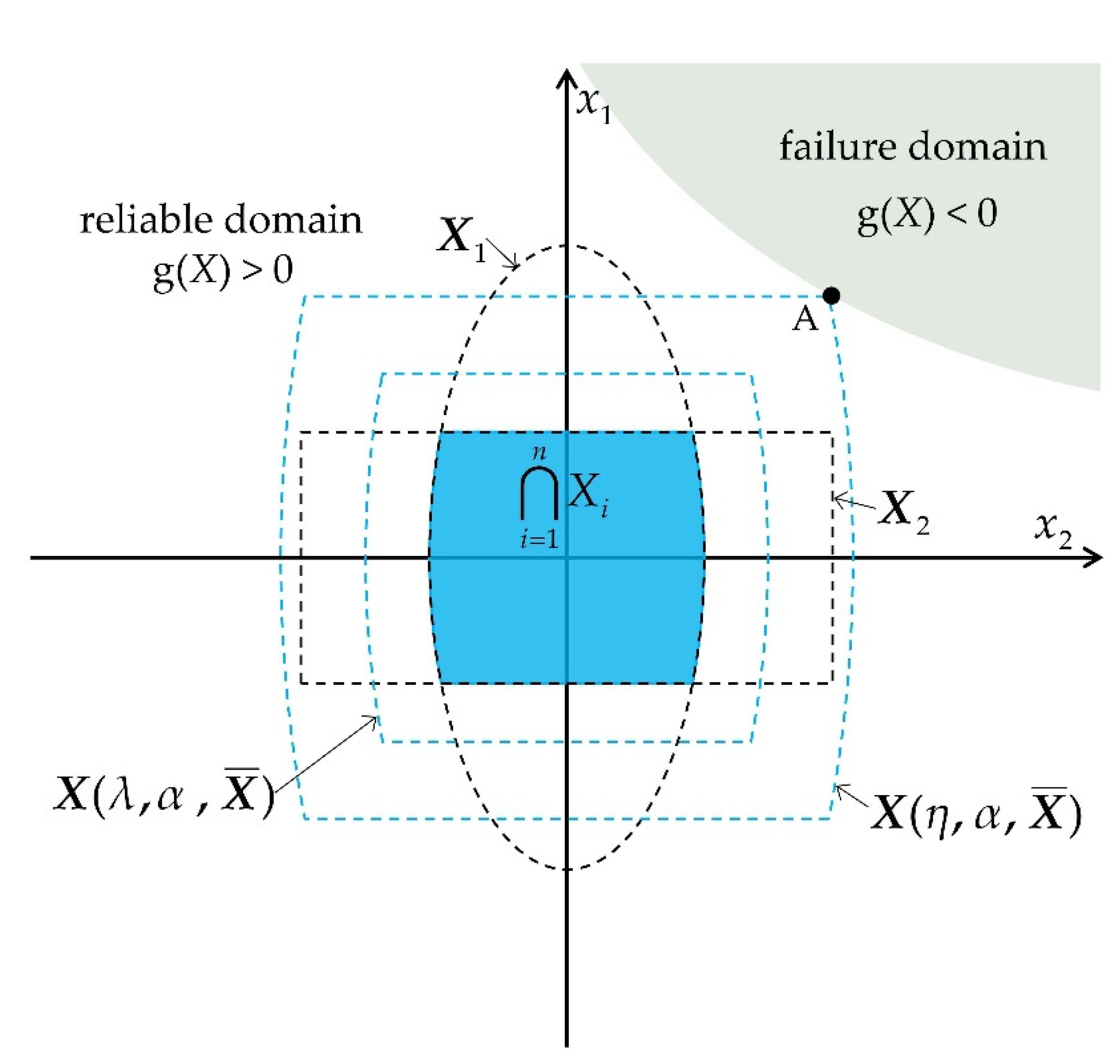Figure 1 shows the non-probabilistic reliability index of a PF considering two uncertain variables in x-space. The failure domain is divided by PF g(X) = 0, and the blue solid area denotes the normalized convex model. It is defined by the intersection of an ellipsoid convex set X₁ and an interval convex set X₂. When the convex set expands to be tangent to the PF, the value of $\lambda$ is the non-probabilistic reliability index η, and the tangent point A is the generalized design point.

Therefore, the minimum $\lambda$ value can be defined as the reliability index η of structural reliability as follows:

$$\begin{array}{c}\eta =\min (\lambda )\hfill \\ s.t.\left\{\begin{array}{c}M=g({\mathit{x}}_1,{\mathit{x}}_2,\dots ,{\mathit{x}}_n)\le 0\hfill \\ {\rho }_i({\mathit{x}}_i,{\overline{\mathit{x}}}_i)\le {\lambda \mathit{\alpha }}_i\hfill \\ {\mathit{X}}_1=({\mathit{x}}_1,\dots ,{\mathit{x}}_n)\in {\mathit{X}}_1({\mathit{\alpha }}_1,{\overline{\mathit{X}}}_1)\hfill \\ \dots \hfill \\ {\mathit{X}}_j=({\mathit{x}}_{n_{j-1}},\dots ,{\mathit{x}}_{n_j})\in {\mathit{X}}_j({\mathit{\alpha }}_j,{\overline{\mathit{X}}}_j)\hfill \\ \dots \hfill \\ {\mathit{X}}_m=({\mathit{x}}_{n_{m-1}+1},\dots ,{\mathit{x}}_{n_m})\in {\mathit{X}}_m({\mathit{\alpha }}_m,{\overline{\mathit{X}}}_m),n_m=n\hfill \end{array}\right.\hfill \end{array}$$

(3)

The index η can be used to simply measure the degree of non-probabilistic reliability to judge whether the structure is in a safe or failure state. The structural reliability problem is then transformed into the problem of finding the optimal solution of η.

The scaling factor of the convex set is used to obtain the optimization formula of η. The optimization formula is obtained by transforming Equation (3) into an unconstrained optimization problem through the penalty method:

$$\min \eta =\lambda +P\cdot \{\max {[0,g(\mathit{X})]}^2+{\displaystyle \sum _{i=1}^m\max {[0,{\rho }_i({\mathit{x}}_i,{\overline{\mathit{x}}}_i)-{\lambda \mathit{\alpha }}_i]}^2}\}$$

(4)

where $\rho (\mathit{x},\overline{\mathit{x}})$ is the functional relation of the convex set model and P is the penalty coefficient, which is generally a large constant. Finally, the non-probabilistic reliability problem is transformed into the problem of finding the optimal solution of Equation (4), which is based on the convex set model X and PF g(X). In other words, Equation (4) can be considered the fitness function of some optimization algorithm, and the optimal solution can be sought.

3. Framework of the Proposed Method

To solve non-probabilistic reliability problems quickly and accurately, there are two possible ways: (1) while ensuring the accuracy of calculation, the time of performing FEA should be reduced as much as possible; that is, the number of calls to the structural PF should be reduced; (2) while ensuring accuracy, the number of samples required by the surrogate model should be reduced as much as possible; that is, the fitting time of the surrogate model should be reduced. As it is also difficult to obtain sufficient samples in practical engineering cases, a dynamic updating mechanism can be used to correct the fitting errors of the surrogate model in local areas on the basis of small samples. The framework of the dynamic surrogate model for non-probabilistic reliability analysis is shown in Figure 2. x* and η are the optimal design point and reliability index searched by the optimization process.

To establish the framework, the dynamic surrogate model needs to include the following three parts: (1) the response surface model; (2) the optimization process; and (3) the dynamic updating process. The first part constructs the response surface model to fit the PF and constructs the fitness function in Equation (4) for non-probabilistic reliability analysis. The second part uses optimization methods to find the optimal value of the fitness function. The third part uses the searched optimal design point as the new center point to construct new sample points and refit the PF if the output does not reach convergence. Finally, the iteration reaches convergence and outputs the optimal solution. These three parts make the computational cost of structural reliability very low. The key technologies of each part of the proposed method are presented in Section 4.

4. Key Technologies of the Proposed Method

4.1. Flexible Construction of the Response Surface with a Small Dataset

To construct the response surface function, a sample dataset related to the uncertain variables must be obtained. The initial sample datasets are constituted by a series of points x_i (i = 1, 2, …, n) and a series of corresponding PF values z_i calculated by FEA. The quality of the sample points directly affects whether the quadratic polynomial response surface can approximate the real PF well.

In traditional structure reliability analysis, the methods of sample point design commonly used in response surface construction are the random sampling design, two-level factorial design [46,47], central composite factorial design [28], Bucher design [48], Latin hypercube sampling design [49], IS design [5,50], and directional simulation [51]. The sampling design method this paper uses is the Bucher design. This is because the number of sample points constructed by the Bucher design grows more slowly than that of other design methods when the number of undetermined variables increases. When the structure is complex and the uncertain variables have a complex high-dimensional form, an increasing number of sample points will reduce the efficiency of fitting the response surface. For example, when there are n factors, the two-level factorial design will construct 2ⁿ sample points, and the central composite factorial design will construct 2ⁿ+ 2n + 1 sample points. Both grow exponentially in number. In contrast, the Bucher design uses the difference set between the central composite factorial design and two-level factorial design, constructing only 2n + 1 sample points, which is linearly increasing. The sampling method in the two-dimensional condition is shown in Figure 3:

In Figure 3, the center of the initial sample points is the position parameter x* = (x₁, x₂, …, x_n). The vertical and horizontal offset distances are kf times the size parameter α_i (interval model k = 1, ellipsoid model k = e_i).

After constructing the initial sample points, the FEM is used to calculate the PF values of the sample points. The obtained function values g(x₁, x₂, …, x_n) and g(x₁, x₂, …, x_i ± kfα_i, …, x_n) and the sample points will be combined by a one-to-one correspondence into 2n + 1 samples of the response surface model.

In this paper, a polynomial response surface is used to fit the PF. When a dynamic fitting strategy is employed, the quadratic polynomial response surface does not need to represent the response of a nonlinear model to multiple uncertainty parameters over the entire feasible region. Instead, it is only necessary to respond to the nonlinear model of the uncertainty parameters near the generalized design point, that is, to realize the local fitting of the response surface near the generalized design point. In local fitting, since the local PF itself is not too complicated, the use of high-order polynomials will not greatly improve the accuracy but will increase a lot of computational costs. So, the use of quadratic polynomials to fit nonlinear PFs is sufficient to achieve high-precision fitting. Simple quadratic polynomials are usually used, as follows:

$$Z=g(\mathit{X})\approx Z_r=\widehat{g}(\mathit{X})=\mathit{A}+{\displaystyle \sum _{i=1}^n{b}_i{\mathit{X}}_i}+{\displaystyle \sum _{i=1}^n{c}_i{\mathit{X}}_i^2+{\displaystyle \sum _{1\le i<j\le n}^n{d}_{ij}{\mathit{X}}_i{\mathit{X}}_j}}$$

(5)

where X are the basic random variables of the structure; a, b_i, c_i, and d_ij are the undetermined coefficients of the polynomial; $g(\mathit{X})$ is the real PF; and $\widehat{g}(\mathit{X})$ is the quadratic polynomial response surface function.

Given the variables X, the corresponding value $\widehat{g}(\mathit{X})$ is calculated by the FEM. Then, the undetermined coefficients can be solved with the following equation:

$$\widehat{g}(\mathit{X})=\lambda \mathit{A}$$

(6)

where $\lambda ={(\mathit{A},\hspace{0.33em}{b}_1,\hspace{0.33em}{b}_2,\hspace{0.33em}\dots ,\hspace{0.33em}{b}_n,\hspace{0.33em}{c}_1,\hspace{0.33em}{c}_2,\hspace{0.33em}\dots ,c_n,\hspace{0.33em}{d}_1,\hspace{0.33em}\dots ,\hspace{0.33em}{d}_n)}^{\mathrm{T}}$, $\widehat{g}(\mathit{X})={({\widehat{g}}_1,\hspace{0.33em}{\widehat{g}}_2,\hspace{0.33em}\dots ,\hspace{0.33em}{\widehat{g}}_{2n+1})}^{\mathrm{T}}$, and A is the coefficient matrix.

To make the response surface fit the real PF better near the checking point, a quadratic polynomial without a cross-product term is usually selected, as follows:

$$Z_r=\widehat{g}(\mathit{X})=\mathit{A}+{\displaystyle \sum _{i=1}^n{b}_i{\mathit{X}}_i}+{\displaystyle \sum _{i=1}^n{c}_i{\mathit{X}}_i^2}$$

(7)

Note that in the non-probabilistic reliability model, if X is a non-probabilistic random variable, the quadratic polynomial response surface function is selected by the above formula. In the case of two random variables X and Y, the response surface model expressed in Equation (7) does not consider the cross product term of random variables; that is, it is equivalent to two variables being independent variables. Therefore, the quadratic polynomial response surface in this case can be obtained by adding the quadratic polynomial constructed by X and the quadratic polynomial constructed by Y, and can be expressed as the following Equation (8):

$$Z_r=\widehat{g}(\mathit{X})=\mathit{A}+{\displaystyle \sum _{i=1}^n{b}_i{\mathit{X}}_i}+{\displaystyle \sum _{i=1}^m{c}_i{Y}_i}+{\displaystyle \sum _{i=1}^n{d}_i{\mathit{X}}_i^2}+{\displaystyle \sum _{i=1}^m{e}_i{Y}_i^2}$$

(8)

The explicit quadratic polynomial response surface model established above is obtained by fitting the implicit PF with sample points. Therefore, the response surface model can be used to replace the PF to divide the structural reliability domain and failure domain and replace the PF to participate in the non-probabilistic reliability analysis of the structure, thus avoiding the impediment of the implicit PF to the structural reliability analysis. Based on the response surface function Equation (8), the optimization problem Equation (4) can be established to determine the non-probabilistic reliability.

4.2. Quickly Searching for the Global Optimal Solution Using the GOA

Due to the diversity of random variables in the structure, the PFs used for structural reliability analysis in engineering structures are often implicit multimodal functions, which means Equation (4) has multiple local optimal solutions. Traditional optimization methods are based on gradient descent to find the global optimum, which often leads to local optimization [52]. Nature-inspired algorithms, such as the genetic algorithm (GA) [53], particle swarm algorithm (PSO) [54], ant colony algorithm (AC) [55], etc., create random input values as candidate optimization schemes. Then, iterative search for the global optimum is achieved by evaluating each scheme, observing the target value, and changing and combining schemes according to the output. However, these algorithms still experience many difficulties in solving complex optimization problems [56]. For example, PSO lacks dynamic adjustment of the search speed and falls into local optimization. GA has a strong global optimization ability but weak local search ability, which makes it difficult to converge quickly. The grasshopper algorithm (GOA) [57] has an adaptively adjusted search speed and can be well combined with non-probabilistic structural reliability solution methods to speed up the solution process [58]. Therefore, GOA becomes the optimization method used in this paper to find the optimal solution of the fitness function Equation (4).

By observing and simulating the collective behavior of grasshopper swarms as they search for food, in 2017, Saremi et al. [57] proposed the grasshopper optimization algorithm (GOA). The basic idea of the GOA is as follows.

The current position of the grasshopper operator X_i can be described as:

$${\mathit{X}}_i=S_i+G_i+{\mathit{A}}_i$$

(9)

where S_i is social interaction, G_i is the force of gravity on the i-th grasshopper, and A_i is the wind advection. These parameters can be defined as follows:

$$S_i={\displaystyle \sum _{j=1,i\ne j}^{N}s(d_{ij}){\widehat{d}}_{ij},\hspace{0.33em}{d}_{ij}=|{\mathit{X}}_i-{\mathit{X}}_j|}$$

(10)

$$G_i=-g{\widehat{e}}_g$$

(11)

$${\mathit{A}}_i=u{\widehat{e}}_w$$

(12)

$$s(r)=f{e}^{\frac{-r}{l}}-e^{-r}$$

(13)

where d_ij is the distance between the i-th and j-th grasshoppers, s is the function shown in Equation (13) to define the strength of social force, and ${\widehat{d}}_{ij}$ is a unit vector of the i-th and j-th grasshoppers. f is the intensity of attraction, and l is the attractive length scale. g is the gravitational constant, and ${\widehat{e}}_g$ is a unit vector towards the center of the Earth. u is a constant drift, and ${\widehat{e}}_w$ is a unit vector in the direction of the wind. Then, the next position of the grasshopper swarm can be defined as follows:

$${\widehat{\mathit{x}}}_i^k=c_1\left({\displaystyle \sum _{j=1}^N{c}_2\frac{u{l}_k-f{l}_k}{2}p\left(d_{ij}^k\right)\frac{{\mathit{x}}_j^k-{\mathit{x}}_j^k}{d_{ij}^k}}\right)+T_g^k$$

(14)

where ${\widehat{\mathit{x}}}_i^k$ indicates the next position of the grasshopper operator x_i in dimension k. $u{l}_k$ and $f{l}_k$ represent the upper and lower bounds of the model in dimension k. If the new positions of some grasshopper operators exceed the upper and lower bounds of the model space, they will be pulled back to the model space. $d_{ij}^k$ represents the distance between grasshopper operator ${\mathit{x}}_i^k$ and grasshopper operator ${\mathit{x}}_j^k$ in dimension k. $T_g^k$ represents the component of the currently found optimal solution in dimension k. c₁ and c₂ are adaptive shrinkage parameters, which can be calculated as:

$$c=c_{\max }-t\frac{c_{\max }-c_{\min }}{t_{\max }}$$

(15)

where t is the current iteration time. c_max and c_min are the maximum and minimum values of the adaptive shrinkage parameters. In this paper, they are set as 1 and 1.0 × 10⁻⁵.

Through the GOA, the proposed method can efficiently search for the optimal solution to Equation (4). The proposed method will gradually approach the generalized design point and the reliability index of non-probabilistic structural reliability.

4.3. Dynamically Updating the Response Surface

After obtaining the initial quadratic polynomial response surface model, the optimal design point can be searched by the GOA. Notably, compared with the initial sample points of the uncertain variables, the optimal design point is much closer to the generalized design point. This indicates that when the structure is impacted by the combination of uncertain variables represented by this optimal point, it is the most likely situation to cause structural failure in the current. This means that this optimal design point is also an effective sample point for the response surface model to learn the characteristics of structural failure. Therefore, we construct an iterative strategy called the dynamic fitting strategy of the response surface: we initialize the response surface model, find the optimal design point, use the searched optimal design point as the new center point to construct new sample points if the outputs do not reach convergence, retrain the response surface model, and find the new optimal design point with the GOA. In addition, since more samples near the generalized design point are found in the dynamic fitting strategy, the response surface model will be fitted near the generalized design point. Therefore, the response surface does not need to be fitted in the entire feasible domain of the PF, thus reducing the cost of fitting. Figure 4 shows the two-dimensional dynamic fitting strategy of the response surface. After two iterations, the response surface model is very close to the PF near the generalized design point.

5. Implementation of the Proposed Method

The proposed method can be implemented through the following steps, as shown in Figure 5.

• Step 1: Create the initial sample points using the Bucher design method. Set x* = (x₁, x₂, …, x_n) as the center of the initial sample points and kfα_i as the offset distance.
• Step 2: Calculate the function values g(x₁, x₂,…, x_n) and g(x₁, x₂,…, x_i ± kfα_i, …, x_n) of each sample point by the FEM. Then, construct 2n + 1 total samples in the dataset.
• Step 3: Solve the undetermined coefficients a, b_i, c_i, d_ij, and e_ij of the quadratic polynomials.
• Step 4: Construct the quadratic polynomial response surface function in the form of Equation (8).
• Step 5: Establish the optimization problem of Equation (4) using the scaling factor of the convex set.
• Step 6: Set the hyper-parameters of the GOA. Search for the global optimal solution of Equation (4) by the GOA to obtain the optimal design point x* and reliability index value η of the current iteration step.
• Step 7: Compare the reliability index value of the current iteration step with that of the previous iteration step. If the convergence conditions are satisfied (|η(i) − η(i-1)| < 10⁻³, where i is the iteration step), stop the iteration and obtain the reliability index. Otherwise, go to Step 8.
• Step 8: Generate new sample points by using the optimal design point x* as the center of Bucher design and calculate the sample FEA value. Then, return to Step 3.

6. Examples and Discussion

To verify the feasibility of this method, four examples—two mathematical examples and two engineering structure examples—are given.

6.1. Example 1

The nonlinear PF of a structure is [37]:

$$g=e^{-{\mathit{x}}_1^2/10}+{({\mathit{x}}_1/5)}^4-{\mathit{x}}_2+2$$

(16)

The variation range of the uncertain variables can be expressed by the following non-probabilistic interval model:

$${\mathit{X}}_1({\mathit{\alpha }}_1,{\overline{\mathit{x}}}_1)=\{{\mathit{x}}_1:|{\mathit{x}}_1-{\overline{\mathit{x}}}_1|\le {\mathit{\alpha }}_1\}$$

(17)

$${\mathit{X}}_2({\mathit{\alpha }}_2,{\overline{\mathit{x}}}_2)=\{{\mathit{x}}_2:|{\mathit{x}}_2-{\overline{\mathit{x}}}_2|\le {\mathit{\alpha }}_2\}$$

(18)

where the position parameters are ${\overline{\mathit{x}}}_1={\overline{\mathit{x}}}_2=0$ and the size parameters are ${\mathit{\alpha }}_1={\mathit{\alpha }}_2=1$.

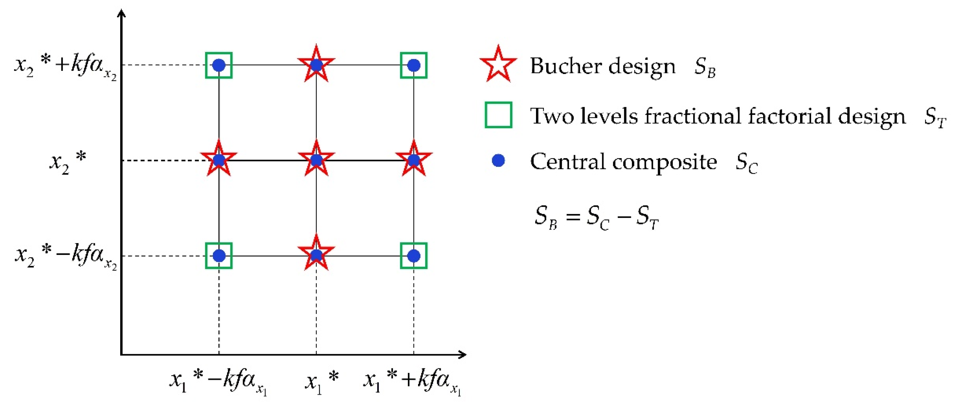
The Bucher experimental design method is used to construct the initial sample points. The position parameter of each variable is taken as the center point. Twice the value of the size parameter is taken as the offset distance of the model.

The parameters of the GOA are set as follows: the dimension is D = 2, the population size is N = 30, the maximum and minimum adaptive shrinkage parameters are c_max = 1 and c_min = 1.0 × 10⁻⁵, the number of iterations is t = 1000, the upper and lower bounds of the model space are ul = 10.0 and fl = −10.0, and the search range of the scaling factor λ is [0, 10].

After three calculation steps, the iteration reaches convergence. The explicit expression of the quadratic polynomial response surface at each iteration step is:

$$\widehat{g}{(\mathit{X})}^{(i)}={\lambda }^{(i)}{\mathit{A}}^{(i)}\hspace{0.33em}\hspace{0.33em}\hspace{0.33em}i=0,\hspace{0.33em}1,\dots ,\hspace{0.33em}3$$

(19)

where $\overline{y}(\mathit{X})$, α, and K in each iteration step are:

Step 1:

$$\begin{gathered} \widehat{g}{(\mathit{X})}^{(0)}=[3.00,\hspace{0.33em}2.91,\hspace{0.33em}4.00,\hspace{0.33em}2.91,\hspace{0.33em}2.00] \\ {\lambda }^{(0)}=[3.00,\hspace{0.33em}0,\hspace{0.33em}-1.00,\hspace{0.33em}-0.0936,\hspace{0.33em}0] \\ {\mathit{A}}^{(0)}=\left[\begin{array}{ccccc}1& 0& 0& 0& 0\\ 1& -1& 0& 1& 0\\ 1& 0& -1& 0& 1\\ 1& 1& 0& 1& 0\\ 1& 0& 1& 0& 1\end{array}\right]; \end{gathered}$$

Step 2:

$$\begin{gathered} \widehat{g}{(\mathit{X})}^{(1)}=[-0.0007,\hspace{0.33em}-0.044,\hspace{0.33em}0.9993,\hspace{0.33em}0.2032,\hspace{0.33em}-1.0007] \\ {\lambda }^{(1)}=[3.4401,\hspace{0.33em}0.5388,\hspace{0.33em}-1.00,\hspace{0.33em}0.0803,\hspace{0.33em}0] \\ {\mathit{A}}^{(1)}=\left[\begin{array}{ccccc}1.0000& -2.5846& 2.5848& 6.6803& 6.6813\\ 1.0000& -3.5846& 2.5848& 12.8495& 6.6813\\ 1.0000& -2.5846& 1.5848& 6.6803& 2.5117\\ 1.0000& -1.5846& 2.5848& 2.5110& 6.6813\\ 1.0000& -2.5846& 3.5848& 6.6803& 12.8509\end{array}\right]; \end{gathered}$$

Step 3:

$$\begin{gathered} \widehat{g}{(\mathit{X})}^{(2)}=[0.0005,\hspace{0.33em}-0.0431,\hspace{0.33em}1.0005,\hspace{0.33em}0.2045,\hspace{0.33em}-0.9995] \\ {\lambda }^{(2)}=[3.4394,\hspace{0.33em}0.5382,\hspace{0.33em}-1.0000,\hspace{0.33em}0.0802,\hspace{0.33em}0] \\ {\mathit{A}}^{(1)}=\left[\begin{array}{ccccc}1.0000& -2.5834& 2.5838& 6.6741& 6.6761\\ 1.0000& -3.5834& 2.5838& 12.8410& 6.6761\\ 1.0000& -2.5834& 1.5838& 6.6741& 2.5085\\ 1.0000& -1.5834& 2.5838& 2.5073& 6.6761\\ 1.0000& -2.5834& 3.5838& 6.6741& 12.8438\end{array}\right]. \end{gathered}$$

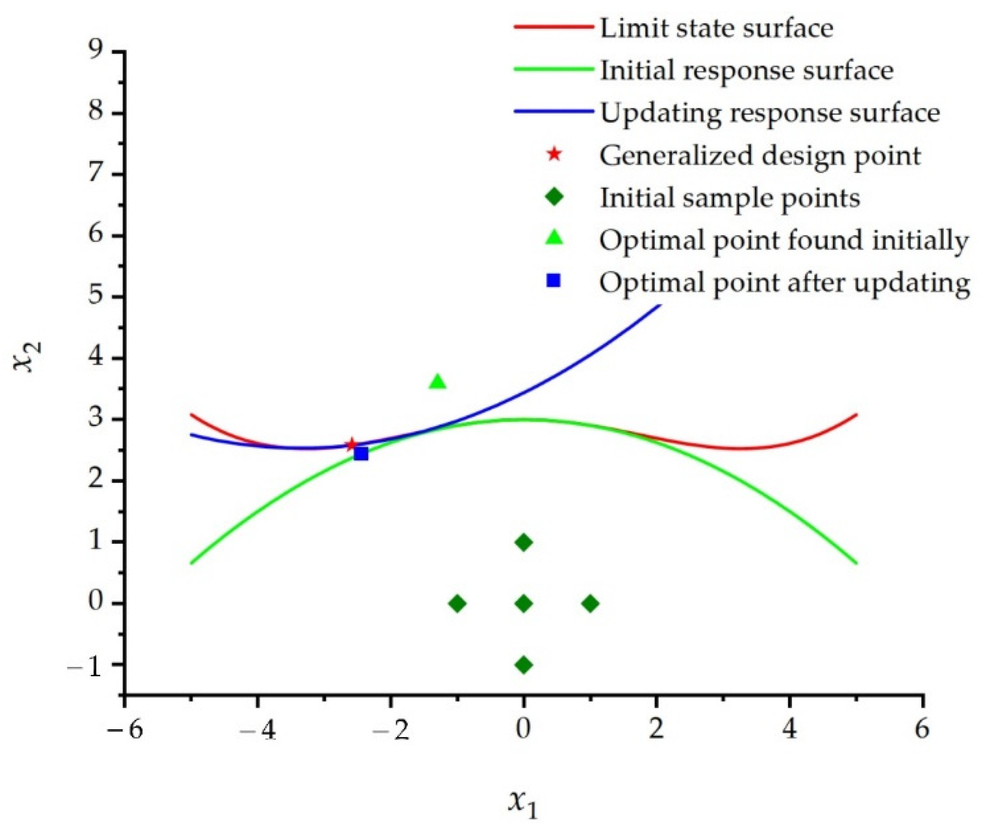
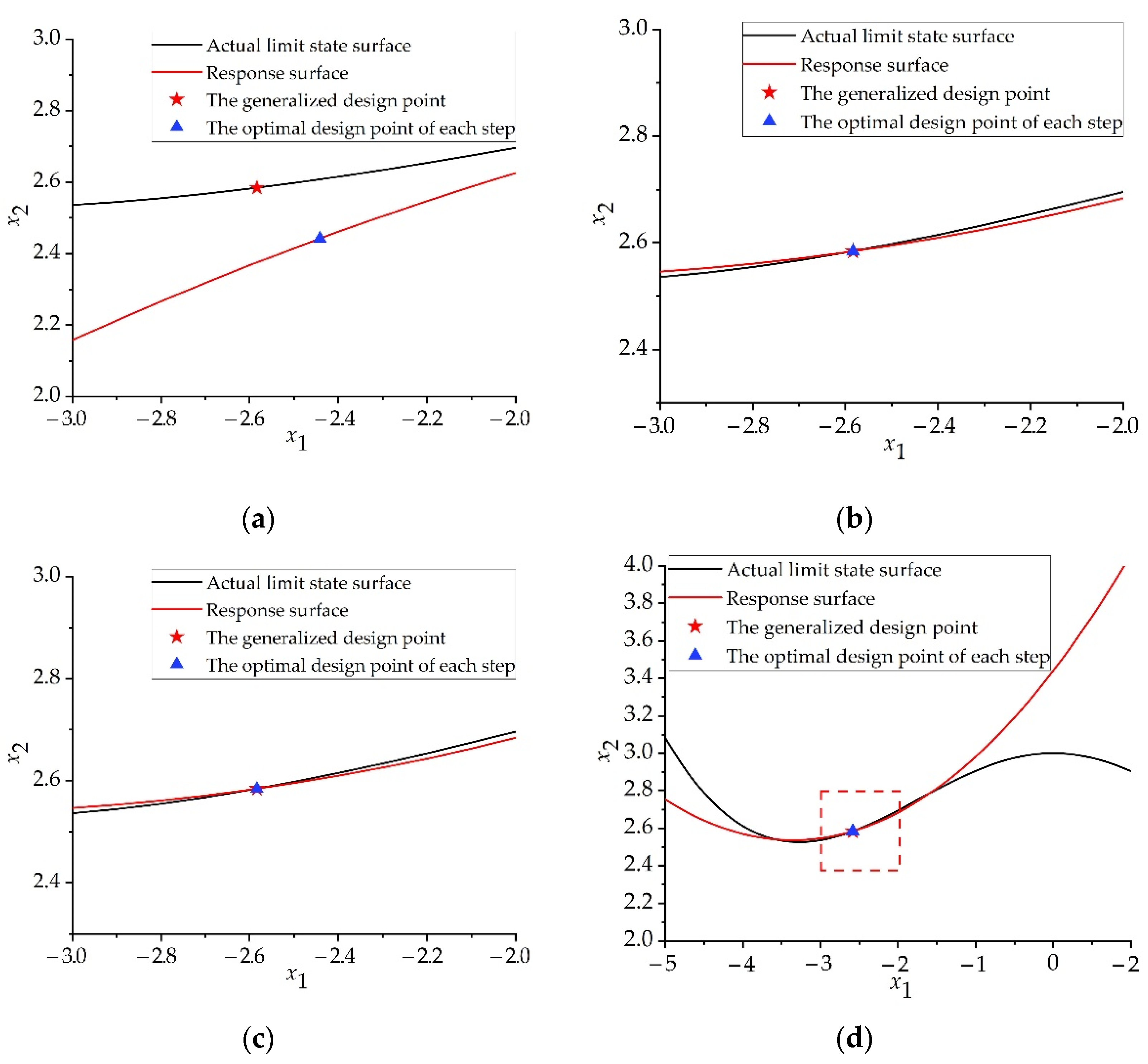
Through the above calculation, the response surface image of each iteration step can be obtained, as shown in Figure 6. Comparing the response surface with the PF and comparing the optimal design point of each iteration step with the generalized design point, it can be seen that the method in this paper can quickly fit the PF and can quickly find the generalized design point. Notably, image (c) is the part in the red box in image (d). This indicates that the proposed method performs local dynamic fitting to the PF in the vicinity of the domain where the generalized design point is located. The proposed method does not focus too greatly on areas far from the generalized design point. Therefore, the fitting process for the PF can be further accelerated on the premise that the generalized design point can be accurately found.

Table 1. Iterative process for solving Example 1.

Iteration Step		I	II	III
Optimal design points	x1*	−2.4417	−2.5834	−2.5835
	x2*	2.4419	2.5838	2.5839
Reliability index η		2.4418	2.5838	2.5838

gives the optimal design points and reliability indices searched by the GOA in each iteration step.

Table 2. Result comparison using different methods for Example 1.

Method	Number of Function Calls	η (×10−3)	Relative Error (%)
MCS	106	2.5846	0
GOA	541	2.5842	0.015
Proposed	16	2.5838	0.031

shows the calculation results of different methods.

In Table 2, the number of function calls f_c can be calculated from the number of sampling points (2n + 1) and the number of iteration steps s. The calculation formula is as follows:

$$f_c=s\times (2n+1)+1$$

(20)

The results of the Monte Carlo simulation (MCS) method with a large number of samples are used as relatively accurate solutions. The result of directly using the GOA to solve the optimization problem of Equation (4) is used as a comparison. Table 1 and Table 2 show two valuable pieces of information. First, the GOA method has higher precision, and the relative error is only 0.015%. Second, the relative error of the proposed method is close to that of the GOA method; however, the number of fitness function calls is significantly lower, only 1/34 that of the GOA method. We place tighter constraints on the convergence conditions of dynamic iterations in our method (|η(i) − η(i − 1)| < 10⁻⁶). The obtained reliability index value is 2.5844, the relative error is reduced to 0.008%, and the number of function calls is 226. It shows that the method in this paper can further increase the accuracy, with a moderate increase in the amount of computation, while still ensuring the computational efficiency. It can be proven that (1) the GOA has a strong optimization capability and can deal with non-probabilistic reliability optimization problems with high precision; (2) the proposed method combines the RSM with the GOA and can improve the efficiency of the solution by reducing the number of calls to the fitness function. The method proposed in this paper has some applicability in solving the non-probabilistic reliability index with the whole interval model of the nonlinear PF of structural reliability.

6.2. Example 2

The PF of a structure is Ref. [37]:

$$g=5{\mathit{x}}_1-\frac{{\mathit{x}}_2{\mathit{x}}_3}{4}$$

(21)

The variation range of the uncertain variables satisfies the following mixed model, which combines the non-probabilistic interval model and super ellipsoid model:

$${\mathit{X}}_1({\mathit{\alpha }}_1,\hspace{0.33em}{\overline{\mathit{x}}}_1)=\{{\mathit{x}}_1:\left|{\mathit{x}}_1-{\overline{\mathit{x}}}_1\right|\le {\mathit{\alpha }}_1\}$$

(22)

$${\mathit{X}}_2({\mathit{\alpha }}_2,\hspace{0.33em}\overline{\mathit{X}})=\{({\overline{\mathit{x}}}_2,\hspace{0.33em}{\overline{\mathit{x}}}_3){\mathit{x}}_1:\frac{{({\mathit{x}}_2-{\overline{\mathit{x}}}_2)}^2}{4}+\frac{{({\mathit{x}}_3-{\overline{\mathit{x}}}_3)}^2}{9}\le {\mathit{\alpha }}_2^2\}$$

(23)

where the position parameters are $\overline{\mathit{X}}=({\overline{\mathit{x}}}_1,\hspace{0.33em}{\overline{\mathit{x}}}_3,\hspace{0.33em}{\overline{\mathit{x}}}_3)=(10,\hspace{0.33em}5,\hspace{0.33em}7)$ and the size parameters are ${\mathit{\alpha }}_1={\mathit{\alpha }}_2=1$.

It is worth noting that GOA has a total of six hyperparameters: the population size N, the maximum number of iterations t, the upper and lower bounds ul and fl of the search, and the maximum and minimum adaptive shrinkage parameters c_max and c_min. The upper and lower search bounds ul and fl represent the search space of the model, which can be reasonably estimated according to the variation range of random variables. The population size N and number of iterations t have similar effects on the operation of the algorithm: when N or t increases, the search operator searches more thoroughly in the entire model space, but if they are too large, it will cause a lot of unnecessary searches, which greatly increases the running time of the algorithm and reduces the efficiency. If N or t is too small, the global optimal solution cannot be searched, which affects the accuracy of the understanding. Therefore, N and the maximum t are two empirical parameters. In general, the more complex the optimization problem to be solved, the greater the N, and the greater the t. The adaptive shrinkage parameter c gradually decreases with the increase in the number of iterations, so that the grasshopper algorithm will not quickly converge to the target. In the early stage of the algorithm, a larger c is set, so that the grasshopper operator is encouraged to perform global optimization, and a small c is set in the later stage of the optimization, so that the grasshopper operator can perform local optimization as much as possible and move toward the target. In addition, the problem dimension D is equal to the number of uncertain variables contained in the optimization problem. Subsequent examples follow the above principles.

The Bucher experimental design method is used to construct the initial sample points. The offset distance of the variables based on the interval model is taken as twice the size parameter value. The offset distance of the variables based on the super ellipsoid model is taken as twice the $e_i{\mathit{\alpha }}_2$ value, where $e=(e_1,\hspace{0.33em}{e}_2)=(2,\hspace{0.33em}3)$.

The parameters of the GOA are set as follows: the dimension is D = 3, the population size is N = 30, the maximum and minimum adaptive shrinkage parameters are c_max = 1 and c_min = 1.0 × 10⁻⁵, the number of iterations is t = 1000, and the upper and lower bounds of the model space are ul = 100.0 and fl = 0.0. The search range of the scaling factor λ is [0, 10].

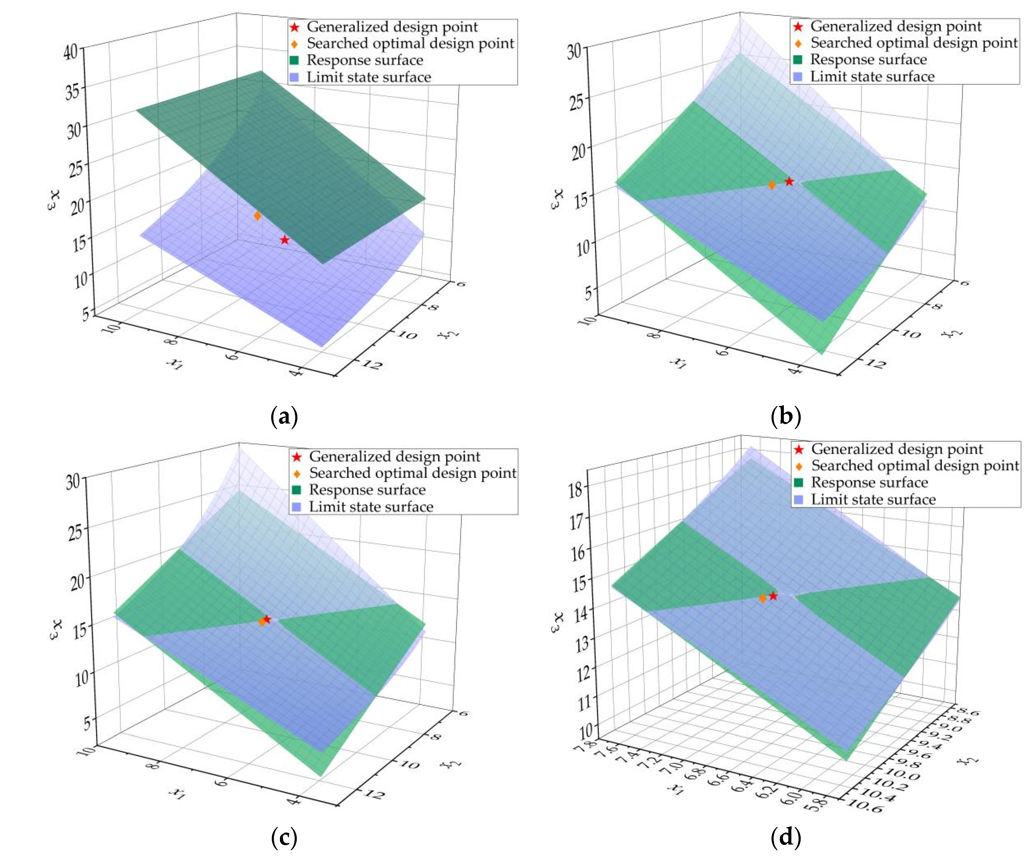
The iteration results of Example 2 are shown in

Table 3. Iterative process for solving Example 2.

Iteration Step		I	II	III	IV
Optimal design points	x1*	5.9263	6.7132	6.7272	6.7219
	x2*	10.774	9.9533	9.4149	9.5114
	x3*	15.6217	13.482	14.2475	14.134
Reliability index η		2.0368	1.6434	1.6384	1.6388

. The comparison results of using different methods are shown in

Table 4. Result comparison using different methods for Example 2.

Method	Number of Function Calls	η	Relative Error (%)
MCS	106	1.6446	-
GOA	506	1.6399	0.286
Proposed	29	1.6388	0.353

, and Figure 7 shows the final response surface $g(\mathit{x})=0$ and the PF $\widehat{g}(\mathit{>x})=0$. The comparison between the final searched optimal point and the generalized design point is also shown.

After four calculation steps, the iteration reaches convergence. In Table 3, with the increase in the iteration steps, the optimal design points and reliability index values tend to become stable gradually. In Table 4, the MCS method is used to simulate 10⁶ calculation results as a relatively accurate solution, and the result of directly using the GOA to solve the optimization problem of Equation (4) is used as a comparison. The error of the proposed method is only 0.353%, and the calculation accuracy is satisfactory. The calculation accuracy of the proposed method is similar to that of the GOA, and the number of function calls is only 29 while the number of function calls of the GOA is 506. The calculation efficiency of the proposed method is obviously higher. Furthermore, Figure 7 shows the dynamic fitting process of the response surface model and the optimal design point of each step. Notably, the range shown in the image in step 4 is smaller than those of the other three steps, and the last step shows that this dynamic fitting strategy makes the response surface model fit the PF very well around the generalized design point. The GOA can quickly determine the optimal design point and makes the iteration quickly reach the convergence condition in four steps.

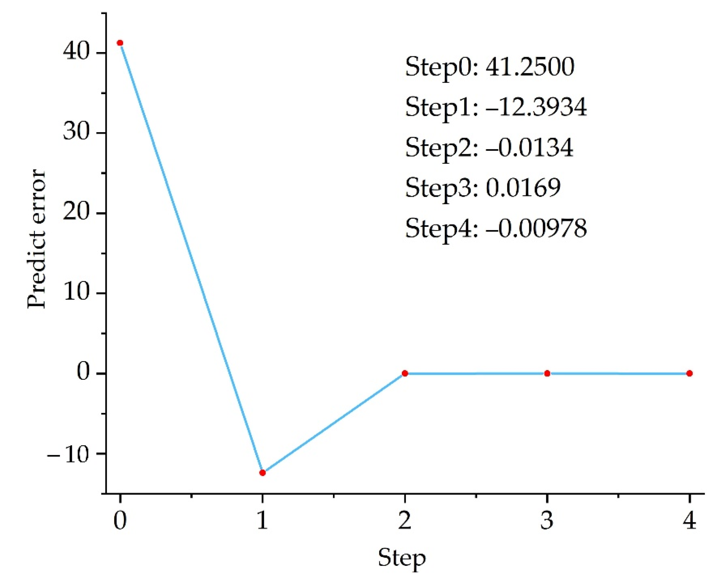
To check the fitting ability of this quadratic polynomial response surface model to the actual PF, after each iteration step, the error between the PF and the response surface model at the optimal design point is calculated (see Figure 8). It can be seen from Figure 8 that the sample points set at the beginning have a large error in the positive direction, and then the dynamic fitting strategy of the proposed method quickly adjusts the parameters, and even a negative error occurs; however, the absolute error is reduced. Finally, according to the errors of the first two steps, the fitting error of the response surface is quickly corrected and reduced, which shows that the surrogate model can fit the implicit PF well.

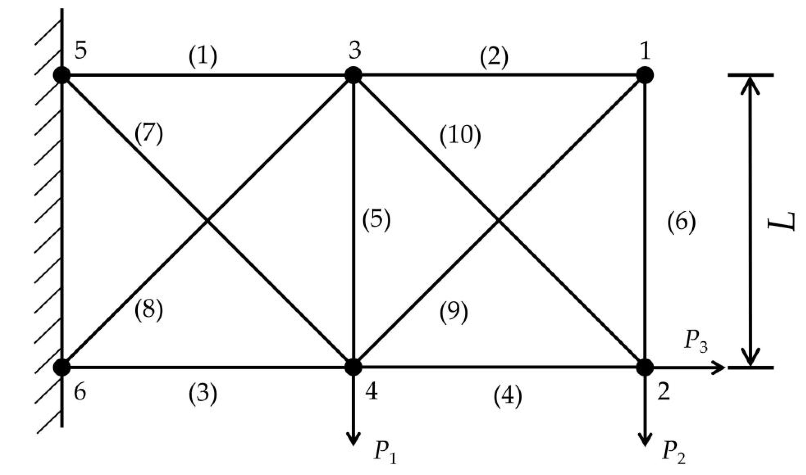
6.3. Example 3: A 10-Truss Girder

Example 3 is a 10-truss girder, as shown in Figure 9. An interval model is used to solve the reliability index with an implicit PF. The length of the horizontal and vertical bars is L, the cross-sectional area of each bar is A_i (i = 1, 2, …, 10), the elastic modulus is E, and the acting positions of the external loads P₁, P₂, and P₃ are shown in the figure. Suppose L, A_i (i = 1, 2, …, 10), E, P₁, P₂, and P₃ are 15 relatively independent interval variables, the position and size parameters of which are shown in

Table 5. Statistical parameters for Example 3.

Random Variable	Unit	Position Parameter	Size Parameter
Ai (i = 1, 2,…, 10)	m2	0.001	0.0002
E	Pa	1 × 1011	1.0 × 1010
P1	N	8 × 105	1.4 × 105
P2	N	1 × 105	1.5 × 104
P3	N	1 × 105	1 × 104
L	m	1	0.01

.

The vertical displacement D(x) of node 2 is considered the intuitive stiffness index in this structure. Therefore, a PF can be established, with D(x) not exceeding 3% of L:

$$g(\mathit{x})=0.06-D(\mathit{x})$$

(24)

The vertical displacement D(x) of node 2 is calculated by the FEA software ANSYS. The parameters of the GOA are set as follows: the dimension is D = 15, the population size is N = 60, the maximum and minimum adaptive shrinkage parameters are c_max = 1 and c_min = 1.0 × 10⁻⁵, the number of iterations is t = 5000, the upper and lower bounds of the model space are ul = 10 and fl = 0.0, and the search range of the scaling factor λ is [0, 10].

The calculation results are shown in

Table 6. Result comparison using different methods for Example 3.

Method	Number of FEA Calls	η	Relative Error (%)
Genetic Algorithm [37]	-	1.4590	-
Linear RSM [37]	135	1.4599	0.060
ANN [37]	280	1.4617	0.190
Proposed	51	1.4611	0.144

. In the table, the search result of the genetic algorithm is taken as the relatively accurate solution [37]. The calculation results of the weighted linear RSM [37] and the ANN [37] are used as a comparison. The result of the weighted linear RSM is the highest, and the accuracy of the proposed method is similar to that of the ANN. However, the number of function calls of the proposed method is significantly lower than those of the above two methods, indicating that the number of FEA calls used in the calculation process of the proposed method is less, so the calculation speed is higher, and the method is more efficient. In another paper by the author of this paper [59], the use of SVM to build a response surface model was proposed and applied to the same structural example. Note that the quadratic polynomial requires fewer samples than SVM, the regression effect is more stable, and the support vector fitting effect is too dependent on the hyperparameters.

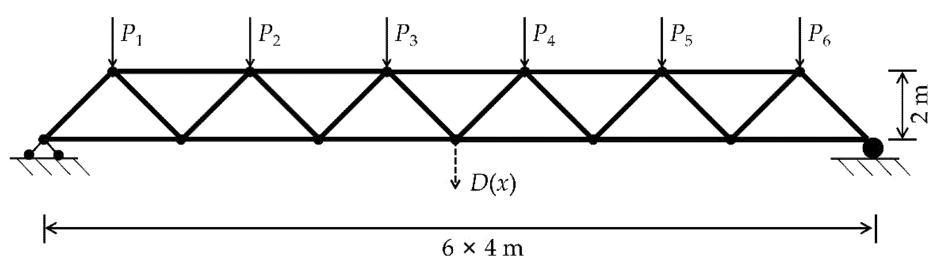
6.4. Example 4: A 23-Truss Girder

Example 4 is a 23-truss girder, as shown in Figure 10 [60]. A mixed model is used to solve the reliability index with an implicit PF. E is the elastic modulus, A is the cross-sectional area, the load P is the uncertain variable of the convex model, and the parameter distributions of the uncertain variables are shown in

Table 7. Statistical parameters for Example 4.

Uncertain Variable	Distribution Type	Unit	Position Parameter	Size Parameter
E1 of horizontal truss	Ellipsoid model	GPa	206.9	1
A1 of horizontal truss	Ellipsoid model	m2	0.002	1
E2 of tilted truss	Ellipsoid model	GPa	206.9	1
A2 of tilted truss	Ellipsoid model	m2	0.002	1
P1	Interval model	kN	49	7.5
P2	Interval model	kN	49	7.5
P3	Interval model	kN	49	7.5
P4	Interval model	kN	49	7.5
P5	Interval model	kN	49	7.5
P6	Interval model	kN	49	7.5

.

The vertical displacement D(x) of the midpoint is considered the intuitive stiffness index in this structure. Therefore, the performance can be established, with D(x) not exceeding 0.15 m:

$$g(\mathit{x})=0.15-D(\mathit{x})$$

(25)

The vertical displacement D(x) of the midpoint is calculated by the FEA software ANSYS. The parameters of the GOA are set as follows: the dimension is D = 10, the population size is N = 80, the maximum and minimum adaptive shrinkage parameters are c_max = 1 and c_min = 1.0 × 10⁻⁵, the number of iterations is t = 6000, the upper and lower bounds of the model space are ul = 20.0 and fl = 0.0, and the search range of the scaling factor λ is [0, 10].

In

Table 8. Result comparison using different methods for Example 4.

Method	Number of FEA Calls	η	Relative Error (%)
MCS	106	2.6013	-
RSM-SQP	111	2.6790	2.987
Proposed	75	2.6102	0.342

, the MCS method is used to simulate 10⁶ calculation results as a relatively accurate solution, and the result of directly using the quadratic polynomial RSM based on sequential quadratic programming (RSM-SQP, implemented using the MATLAB toolbox) to solve the optimization problem of Equation (4) is used as a comparison. It can be seen that in terms of both the number of function calls and the accuracy of the reliability index, the proposed method is better than RSM-SQP.

7. Conclusions

This paper presents a grasshopper optimization algorithm-based RSM for non-probabilistic structural reliability analysis with an implicit PF. The main conclusions are as follows:

1.

By conducting the proposed method, the reliability index of a structure can be quickly found with fewer function calls. The error self-correction fitting of the response surface model near the generalized design point is achieved. This significantly reduces the number of calls to the PF in the calculation process and avoids the decrease in the solution speed caused by the global fitting of the response surface model. Compared with MCS and other methods, the proposed method is more suitable for performing non-probabilistic reliability analysis with an implicit PF, especially for non-probabilistic reliability analysis of complex engineering structures with high computational accuracy requirements; however, it has lower time consumption because there are fewer calls to the FEA.

2.

The proposed method is nonintrusive. An existing structural analysis program or FEA software can be directly invoked to carry out the proposed method. It can be easily applied by structural engineers without any modification to structural analysis programs or FEA software.

The efficiency and convenience of the proposed method make it a new way of quickly solving reliability problems for structures with implicit PFs. However, this research is suitable only for reliability analysis with a unique optimal solution. The case of multiple solutions needs further research. The method in this paper is not suitable for structures with multiple optimal solutions or structures with discontinuous PFs. In the above cases, the proposed method will not be able to obtain all possible results. In addition, in the reliability calculation of more complex engineering structures, the quadratic polynomial response surface model has great limitations, and it is impossible to fit the high-order features of the structural limit state surface from the sample points. Therefore, the following work will focus on applying different response surface models with higher fitting accuracy and more efficient optimization methods to the dynamic fitting framework proposed in this paper.

References

1. Keshtegar, B.; Seghier, M.E.A.B.; Zio, E.; Correia, J.A.; Zhu, S.P.; Trung, N.T. Novel efficient method for structural reliability analysis using hybrid nonlinear conjugate map-based support vector regression. Comput. Methods Appl. Mech. Eng. 2021, 381, 113818. [Google Scholar] [CrossRef]
2. Zhu, S.-P.; Keshtegar, B.; Seghier, M.E.A.B.; Zio, E.; Taylan, O. Hybrid and enhanced PSO: Novel first order reliability method-based hybrid intelligent approaches. Comput. Methods Appl. Mech. Eng. 2022, 393, 114730. [Google Scholar] [CrossRef]
3. Xiao, M.; Zhang, J.; Gao, L.; Lee, S.; Eshghi, A.T. An efficient Kriging-based subset simulation method for hybrid reliability analysis under random and interval variables with small failure probability. Struct. Multidiscip. Optim. 2019, 59, 2077–2092. [Google Scholar] [CrossRef]
4. Zio, E.; Pedroni, N. An optimized Line Sampling method for the estimation of the failure probability of nuclear passive systems. Reliab. Eng. Syst. Saf. 2010, 95, 1300–1313. [Google Scholar] [CrossRef] [Green Version]
5. Au, S.K.; Beck, J.L. A new adaptive importance sampling scheme for reliability calculations. Struct. Saf. 1999, 21, 135–158. [Google Scholar] [CrossRef]
6. Yang, D.; Yi, P. Chaos control of performance measure approach for evaluation of probabilistic constraints. Struct. Multidiscip. Optim. 2008, 38, 83–92. [Google Scholar] [CrossRef]
7. Keshtegar, B.; Chakraborty, S. An efficient-robust structural reliability method by adaptive finite-step length based on Armijo line search. Reliab. Eng. Syst. Saf. 2018, 172, 195–206. [Google Scholar] [CrossRef]
8. Keshtegar, B.; Meng, Z. A hybrid relaxed first-order reliability method for efficient structural reliability analysis. Struct. Saf. 2017, 66, 84–93. [Google Scholar] [CrossRef]
9. Cremona, C.; Gao, Y. The possibilistic reliability theory: Theoretical aspects and applications. Struct. Saf. 1997, 19, 173–201. [Google Scholar] [CrossRef]
10. Zhu, S.-P.; Keshtegar, B.; Chakraborty, S.; Trung, N.-T. Novel probabilistic model for searching most probable point in structural reliability analysis. Comput. Methods Appl. Mech. Eng. 2020, 366, 113027. [Google Scholar] [CrossRef]
11. Johari, A.; Mehrabani, L. System probabilistic model of rock slope stability considering correlated failure modes. Comput. Geotech. 2017, 81, 26–38. [Google Scholar] [CrossRef]
12. Su, G.; Peng, L.; Hu, L. A Gaussian process-based dynamic surrogate model for complex engineering structural reliability analysis. Struct. Saf. 2017, 68, 97–109. [Google Scholar] [CrossRef]
13. Elishakoff, I. Essay on uncertainties in elastic and viscoelastic structures: From AM. Freudenthal’s criticisms to modern convex modeling. Comput. Struct. 1995, 56, 871–895. [Google Scholar] [CrossRef]
14. Bai, Y.; Han, X.; Jiang, C.; Bi, R. A response-surface-based structural reliability analysis method by using non-probability convex model. Appl. Math. Model. 2014, 38, 3834–3847. [Google Scholar] [CrossRef]
15. Ben-Haim, Y. Convex Models of Uncertainty in Radial Pulse Buckling of Shells. J. Appl. Mech. 1993, 60, 683–688. [Google Scholar] [CrossRef]
16. Elishakoff, I.; Elisseeff, P.; Glegg, S. Non-probabilistic convex theoretic modeling of scatter in material properties. AIAA J. 1994, 32, 843–849. [Google Scholar] [CrossRef]
17. Sexsmith, R.G. Probability-based safety analysis—Value and drawbacks. Struct. Saf. 1999, 21, 303–310. [Google Scholar] [CrossRef]
18. Qiu, Z.; Elishakoff, I. Antioptimization of structures with large uncertain-but-non-random parameters via interval analysis. Comput. Methods Appl. Mech. Eng. 1998, 152, 361–372. [Google Scholar] [CrossRef]
19. Wang, X.; Qiu, Z.; Elishakoff, I. Non-probabilistic set-theoretic model for structural safety measure. Acta Mech. 2008, 198, 51–64. [Google Scholar] [CrossRef]
20. Wang, X.; Wang, L.; Elishakoff, I.; Qiu, Z. Probability and convexity concepts are not antagonistic. Acta Mech. 2011, 219, 45–64. [Google Scholar] [CrossRef]
21. Jiang, C.; Zhang, Q.F.; Han, X.; Liu, J.; Hu, D.A. Multidimensional parallelepiped model-a new type of non-probabilistic convex model for structural uncertainty analysis. Int. J. Numer. Methods Eng. 2015, 103, 31–59. [Google Scholar] [CrossRef]
22. Pantelides, C.P.; Ganzerli, S. Design of Trusses Under Uncertain Loads Using Convex Models. J. Struct. Eng. 1998, 124, 318–329. [Google Scholar] [CrossRef]
23. Jiang, C.; Han, X.; Lu, G.; Liu, J.; Zhang, Z.; Bai, Y. Correlation analysis of non-probabilistic convex model and corresponding structural reliability technique. Comput. Methods Appl. Mech. Eng. 2011, 200, 2528–2546. [Google Scholar] [CrossRef]
24. Kang, Z.; Zhang, W. Construction and application of an ellipsoidal convex model using a semi-definite programming formu-lation from measured data. Comput. Methods Appl. Mech. Eng. 2016, 300, 461–489. [Google Scholar] [CrossRef]
25. Guo, S.; Lu, Z. A non-probabilistic robust reliability method for analysis and design optimization of structures with uncertain-but-bounded parameters. Appl. Math. Model. 2015, 39, 1985–2002. [Google Scholar] [CrossRef]
26. Cao, L.; Liu, J.; Xie, L.; Jiang, C.; Bi, R. Non-probabilistic polygonal convex set model for structural uncertainty quantification. Appl. Math. Model. 2020, 89, 504–518. [Google Scholar] [CrossRef]
27. Wang, P.; Yang, L.; Zhao, N.; Li, L.; Wang, D. A New SORM Method for Structural Reliability with Hybrid Uncertain Variables. Appl. Sci. 2020, 11, 346. [Google Scholar] [CrossRef]
28. Faravelli, L. Response-Surface Approach for Reliability Analysis. J. Eng. Mech. 1989, 115, 2763–2781. [Google Scholar] [CrossRef]
29. Liu, M.; Wang, X.; Zhu, X.; Chen, W.; Li, X. Non-probabilistic Integrated Reliability Analysis of Structures with Fuzzy Interval Uncer-tainties using the Adaptive GPR-RS Method. KSCE J. Civ. Eng. 2019, 23, 3978–3992. [Google Scholar] [CrossRef]
30. Luo, D.; Huang, J.; Su, G.; Tao, H. A dynamic Gaussian process surrogate model-assisted particle swarm optimisation algorithm for expensive structural optimisation problems. Eur. J. Environ. Civ. Eng. 2022, 1–21. [Google Scholar] [CrossRef]
31. Li, J.; Xiu, D. Evaluation of failure probability via surrogate models. J. Comput. Phys. 2010, 229, 8966–8980. [Google Scholar] [CrossRef]
32. Janouchová, E.; Sýkora, J.; Kučerová, A. Polynomial chaos in evaluating failure probability: A comparative study. Appl. Math. 2018, 63, 713–737. [Google Scholar] [CrossRef]
33. Ghanem, R.; Red-Horse, J. Polynomial chaos: Modeling, estimation, and approximation. In Handbook of Uncertainty Quantification; Springer: Cham, Switzerland, 2016; pp. 1–31. [Google Scholar]
34. Landi, F.; Marsili, F.; Friedman, N.; Croce, P. gPCE-Based Stochastic Inverse Methods: A Benchmark Study from a Civil Engi-neer’s Perspective. Infrastructures 2021, 6, 158. [Google Scholar] [CrossRef]
35. Richard, B.; Cremona, C.; Adelaide, L. A response surface method based on support vector machines trained with an adaptive experimental design. Struct. Saf. 2012, 39, 14–21. [Google Scholar] [CrossRef]
36. Zhao, H.; Ru, Z.; Chang, X.; Yin, S.; Li, S. Reliability analysis of tunnel using least square support vector machine. Tunn. Undergr. Space Technol. 2014, 41, 14–23. [Google Scholar] [CrossRef]
37. Liu, C. Research on Reliability Analysis and Design of Complex Structure. Ph.D. Thesis, Northwestern Polytechnical University, Xi’an, China, December 2006. [Google Scholar]
38. Gomes, H.M.; Awruch, A.M.; Lopes, P.A.M. Reliability based optimization of laminated composite structures using genetic algorithms and Artificial Neural Networks. Struct. Saf. 2011, 33, 186–195. [Google Scholar] [CrossRef]
39. Herbert, M.; Awruch, M. Comparison of response surface and neural network with other methods for structural reliability analysis. Struct. Saf. 2004, 26, 49–67. [Google Scholar]
40. Claudio, M.; José, A. Fast Monte Carlo reliability evaluation using support vector machine. Reliab. Eng. Syst. Saf. 2002, 76, 237–243. [Google Scholar]
41. Lü, Q.; Low, B.K. Probabilistic analysis of underground rock excavations using response surface method and SORM. Comput. Geotech. 2011, 38, 1008–1021. [Google Scholar] [CrossRef]
42. Ben-Haim, Y.; Elishakoff, I. Discussion on: A non-probabilistic concept of reliability. Struct. Saf. 1995, 17, 195–199. [Google Scholar] [CrossRef]
43. Qiu, Z.; Wang, X. Interval analysis method and convex models for impulsive response of structures with uncertain-but-bounded external loads. Acta Mech. Sin. 2006, 22, 265–276. [Google Scholar] [CrossRef]
44. Ruigang, Y.; Wenzhao, L.; Guangli, Z.; Yuzhen, L.; Weichen, J. Interval non-probabilistic time-dependent reliability analysis of boom crane structures. J. Mech. Sci. Technol. 2021, 35, 535–544. [Google Scholar] [CrossRef]
45. Zhan, J.; Luo, Y.; Zhang, X.; Kang, Z. A general assessment index for non-probabilistic reliability of structures with bounded field and parametric uncertainties. Comput. Methods Appl. Mech. Eng. 2020, 366, 113046. [Google Scholar] [CrossRef]
46. Wong, F.S. Slope Reliability and Response Surface Method. J. Geotech. Eng. 1985, 111, 32–53. [Google Scholar] [CrossRef]
47. Wong, F.S. Uncertainties in Dynamic Soil-Structure Interaction. J. Eng. Mech. 1984, 110, 308–324. [Google Scholar] [CrossRef]
48. Bucher, C.G. A fast and efficient response surface approach for structural reliability problems. Struct. Saf. 1990, 7, 57–66. [Google Scholar] [CrossRef]
49. Wu, Z.; Wang, S.; Ge, X. Application of Latin hypercube sampling technique to slope reliability analysis. Rock Soil Mech. 2010, 31, 1047–1054. [Google Scholar]
50. Deng, J.; Gu, D.; Li, X.; Yue, Z.Q. Structural reliability analysis for implicit performance functions using artificial neural network. Struct. Saf. 2005, 27, 25–48. [Google Scholar] [CrossRef]
51. Ditlevsen, O.; Olesen, R.; Mohr, G. Solution of a class of load combination problems by directional simulation. Struct. Saf. 1986, 4, 95–109. [Google Scholar] [CrossRef]
52. Mirjalili, S.; Jangir, P.; Saremi, S. Multi-objective ant lion optimizer: A multi-objective optimization algorithm for solving engineering problems. Appl. Intell. 2016, 46, 79–95. [Google Scholar] [CrossRef]
53. Koza, J.R. Genetic programming as a means for programming computers by natural selection. Stat. Comput. 1994, 4, 87–112. [Google Scholar] [CrossRef]
54. Poli, R.; Kennedy, J.; Blackwell, T. Particle swarm optimization. Swarm Intell. 2007, 1, 33–57. [Google Scholar] [CrossRef]
55. Blum, C. Ant colony optimization: Introduction and recent trends. Phys. Life Rev. 2005, 2, 353–373. [Google Scholar] [CrossRef] [Green Version]
56. Boussaïd, I.; Lepagnot, J.; Siarry, P. A survey on optimization metaheuristics. Inf. Sci. 2013, 237, 82–117. [Google Scholar] [CrossRef]
57. Saremi, S.; Mirjalili, S.; Lewis, A. Grasshopper Optimisation Algorithm: Theory and application. Adv. Eng. Softw. 2017, 105, 30–47. [Google Scholar] [CrossRef] [Green Version]
58. Zhang, G.; Hamzehkolaei, N.S.; Rashnoozadeh, H.; Band, S.S.; Mosavi, A. Reliability assessment of compressive and splitting tensile strength prediction of roller compacted concrete pavement: Introducing MARS-GOA-MCS. Int. J. Pavement Eng. 2021, 1–18. [Google Scholar] [CrossRef]
59. Yang, Y.; Sun, W.; Su, G. A Novel Support-Vector-Machine-Based Grasshopper Optimization Algorithm for Structural Relia-bility Analysis. Buildings 2022, 12, 855. [Google Scholar] [CrossRef]
60. Lee, S.H.; Kwak, B.M. Response surface augmented moment method for estimating the reliability of long span suspension bridges. Finite Elem. Anal. Des. 2010, 46, 658–667. [Google Scholar]
Figure 1. Schematic of the non-probabilistic reliability index based on a convex set model.
Buildings 12 01061 g001
Figure 2. Framework of the proposed method.
Buildings 12 01061 g002
Figure 3. Two-dimensional schematic of the Bucher design.
Buildings 12 01061 g003
Figure 4. Sketch of the two-dimensional dynamic fitting strategy for the response surface.
Buildings 12 01061 g004
Figure 5. Implementation flowchart of the proposed method.
Buildings 12 01061 g005
Figure 6. The steps of fitting the response surface to the limit state surface and searching for the optimal design point: (a) Step 1, (b) step 2, (c) step 3, (d) the entire feasible domain of step 3.
Buildings 12 01061 g006
Figure 7. Fitting process of the response surface in each step: (a) step 1, (b) step 2, (c) step 3, (d) step 4.
Buildings 12 01061 g007
Figure 8. Absolute errors of the predict values of optimal design points.
Buildings 12 01061 g008
Figure 9. The 10-truss girder in Example 3.
Buildings 12 01061 g009
Figure 10. Twenty-three-truss girder.
Buildings 12 01061 g010