1. Introduction
Non-intrusive load decomposition uses the measurement of the total power data of the household electricity meter to estimate the decomposition in order to obtain the electricity consumption of the common individual appliances in the household [
1]. The decomposition results can help monitor the electricity consumption of the household, help users reduce consumption while identifying faulty appliances and investigating the usage of appliances to maximize efficient grid distribution, and help plan scientific electricity consumption schemes and improve electricity consumption efficiency, thus achieving the purpose of saving electricity and energy and reducing consumption [
2].
Nowadays, a lot of academic achievements have been made in the research on non-intrusive load decomposition. There are two main categories of research methods on non-intrusive load decomposition: one is the event-based load decomposition method, while the other is the load model-based load decomposition method.
In 1982, Hart from MIT first proposed the concept of “non-intrusive load monitoring” [
3]; he extracted the steady-state features for power decomposition and designed a simple non-intrusive load monitoring system. Instead of using individual sockets for specific devices, NILM applies intelligent algorithms to analyze and break down meter data without disturbing the end user, which is more economical and acceptable [
4]. However, the method lacked universality and was only applicable to high-power devices, such as air conditioners, heaters, etc. If additional devices are added, it is difficult to discern the differences between appliances, and there are limitations. Its earliest work dates back to the early 1990s. In those days, most electrical appliances were switching devices (e.g., fans, lamps, heaters, ovens, coolers, etc.), so it was a logical idea for such a monitoring system to be set up. Over time, more complex multi-state devices were introduced, such as computers, printers, etc. In 2007, Chang proposed a BP classifier-based load decomposition model after comparing the adaptation scenarios of various transient and steady-state load features [
5]. In 2009, Berges and Scott were inspired by the detection of load events from the main home circuit and developed a generalized likelihood ratio test for the detection of new load events, which improved the load decomposition of residential electricity with some improvements [
6]. The literature [
7] draws on the method of matrix solving in mathematics to build a load decomposition model by using an efficient sparse optimization matrix approach to solve for accurate non-intrusive load decomposition for residential electricity. In the literature [
8], in addition to adding charge features, other non-traditional charge features such as load running time, load running state, frequency of use distribution, and correlation between appliances were used for analysis to improve the decomposition performance of the algorithm. In 2012, Kolter combined Hidden Markov Models with load decomposition to learn the operating state of individual appliances, further improving the accuracy [
9]. In 2015, Yang proposed a load event detection model based on the adaptive cardinality algorithm, which led to a certain degree of improvement in event detection accuracy [
10]. The literature [
11] describes and analyzes the current non-intrusive load disaggregation techniques in detail and gives alternative research ideas. In recent years, scholars have proposed many event-based decomposition algorithms, which have led to the continuous improvement of the accuracy of non-intrusive load decomposition by this class of methods. However, it is only for data samples with a high sampling rate, so many event detection algorithms have certain limitations.
For research on load model-based decomposition methods, Batra has developed an open-source software platform, NILMTK, with example tutorials that greatly improve the speed of researchers in developing new algorithms [
12]. At present, the methods based on artificial features are mainly solved by combinatorial optimization method [
13] and the Markov model [
14]. Kim [
7] proposed a combined multi-factor Hidden Markov and load decomposition model that uses a single Hidden Markov chain of devices and then tensor multiplication to obtain the Hidden Markov. In the decomposition stage, the multi-factor Hidden Markov chain will find the optimal combination based on the given total power data, but the algorithm is susceptible to local optimal solutions for hidden state estimation and therefore does not yield accurate appliance power values. Parson used unsupervised learning to decompose the high frequency power of the appliance and verified, through data testing, its effectiveness [
15].
However, traditional algorithms that separate appliance power by finding the difference terms between appliances are not only difficult to decompose but are also susceptible to interference between similar appliance powers [
16]. If an inappropriate classifier is chosen—for example, by over-emphasizing a particular electrical feature—a number of errors may arise, ultimately leading to incorrect decomposition [
17]. In contrast, non-intrusive load decomposition by deep learning algorithms can further improve the decomposition accuracy, identify electrical appliances more accurately, and enhance the generalization performance, which is of great research significance in promoting the development of non-intrusive load decomposition technology. The method based on deep learning does not need to construct load features manually. Deep learning can automatically extract features according to the needs of tasks, which is also the biggest difference between the load decomposition method based on deep learning and the traditional load decomposition method based on features. The literature [
18] experimented with deep learning algorithms in the field of load decomposition, using artificial neural networks, recurrent neural networks, and noise-reducing self-encoders for experiments and comparing them with Professor Hart’s combined optimization algorithm, confirming that the noise-reducing self-encoder was the best. Xia et al. [
19] used long- and short-term memory recurrent neural networks to model different loads and effectively improved the decomposition accuracy by learning the correlation information between the load data, but the training time was too long. The literature [
20] proposed the use of CNN to extract load features, which can reduce the computational cost. Zhang used CNN to implement sequence-to-sequence and sequence-to-point non-invasive load decomposition, and the main innovation is that the model structure uses the total power data window to predict the output value, and, compared with other deep learning algorithms, the method in the paper has very good results on electrical devices [
21]. Ali Sharif Razavian also pointed out the results of work that specifically optimized CNN representations for different tasks/datasets, resulting in better results [
22]. Kaselimi et al. [
23] proposed a Bayesian optimized bidirectional LSTM regression model for non-intrusive load monitoring, which introduces a Bayesian optimization framework to select the best configuration of the proposed regression model in order to improve performance. Verma et al. [
24] proposed a multi-label LSTM autoencoder for non-intrusive appliance load monitoring to solve the problem of considering the time variability of input signals in the multi-label classification framework. Zhou et al. [
25] proposed a CNN LSTM hybrid deep learning model for non-intrusive load monitoring, which combines a convolutional neural network (CNN) with a long- and short-term memory network (LSTM) to fully mine the spatio-temporal characteristics of the load data and improve the accuracy of the decomposition. However, the current methods based on LSTM can effectively extract the time-series dependency of sequences, but the ability to extract load characteristics is limited, and the current LSTM model needs to be trained for different loads, which leads to low operation efficiency.
The existing non-intrusive load decomposition is mainly based on traditional load features to establish the decomposition model of an electric load, while the traditional feature extraction method cannot achieve high-precision real-time decomposition, and it has a difficult time meeting the current market demand for the intelligent development of the power grid. Current energy decomposition methods extract features from sequences, a process that tends to lead to the loss of load features and difficulties in detection, resulting in low recognition rates for low-usage appliances [
26]. With the rapid development of deep learning algorithms, more and more models have begun to be applied to the task of non-invasive load decomposition. However, the deepening of the model structure leads to too many parameters, a slow training speed, and a high calculation cost, which leads to the phenomenon of feature redundancy and reduced learning ability. To address the above challenges, this paper constructs an improved non-intrusive load decomposition method based on deep learning models. The non-intrusive load decomposition model based on long- and short-term memory multi-output networks is proposed. In this network, an improved multi-scale fusion residual module is proposed to extract the basic load characteristics, and the LSTM cycle unit is proposed to extract the time series information. Through the combination with the reorganization of the input data, the effect of feature reuse is achieved and respectively input into multiple branches. Then, the deep LSTM cycle unit retains the effective load characteristics in the network and outputs the predicted power values of multiple target loads. The overall model structure reduces the difficulty of network optimization. The structure can decompose the target load power while ensuring the load decomposition accuracy so as to reduce the calculation cost and improve the training efficiency. This paper presents an in-depth study of non-intrusive load decomposition for residential electricity using an experimental analysis and validation of electricity data from the foreign public WikiEnergy dataset and the UK-DALE dataset [
27]. Based on the evaluation and analysis of the experimental results in terms of accuracy, recall, and F1 value respectively, the analysis and validation of the experimental results show that the decomposition effect of the proposed method on the test set is better than that of the traditional algorithm.
2. Proposed Method
From a neural network perspective, the problem of non-intrusive power load disaggregation for residential electricity consumption can be explained in this way. Assuming that
represents the sum of the active power consumption of all electrical devices in a household at a given time, this can then be expressed as Equation (1).
where
represents the active power value of the
th residential electrical appliance at moment
,
represents the number of electrical appliances, and
represents the model noise. Thus, the non-intrusive load disaggregation model can represent the solution to the problem of finding
for all electrical equipment under the condition that
is known.
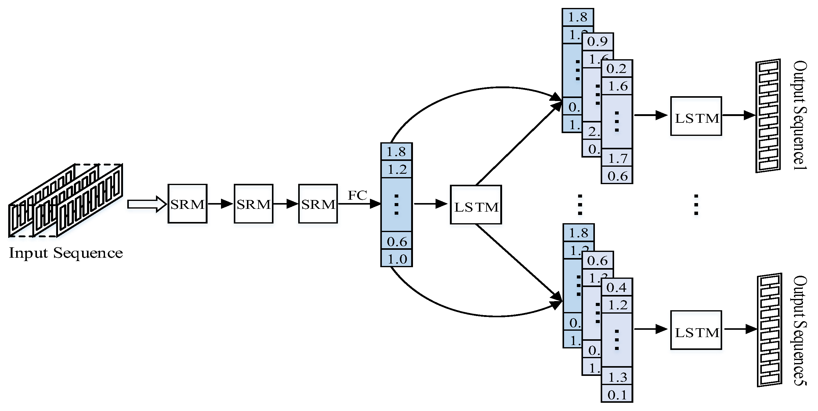
The M-LSTM designed in this work can decompose the total input power data into the power of multiple targets loading at the same time, thus avoiding the repeated training of the network model and saving computational resources, which improves training efficiency. The overall structure of the model is shown in
Figure 1. The network model includes a basic convolutional layer, a multi-scale-fused Residual Module (SRM), an LSTM loot unit, a Fully Connected Layer (FC), etc. In the data pre-processing process, the data sliding window is uniformly set to 128 units in order to meet the window size requirements for all loads. All of the processed data are combined into a training set and input into the network, which is subjected to a basic
convolution containing Relu nonlinear activation, Batch Normalization, and other operations to obtain the base feature map. The final feature map with a large number of loading features is obtained by stacking three multi-scale fusion residual modules, which are stretched into a one-dimensional vector by a fully connected operation (FC layer) and fed into an LSTM recurrent unit. Inspired by residual convolutional neural networks and densely connected neural networks, the “transfer” of load features also draws on the idea of “cross-layer connectivity”. While traditional neural networks tend to be progressive in structure, i.e., they go deeper layer by layer, the network layers of a neural network can also be passed across—in other words, a layer of the network can be derived from the features of the previous layer and can also receive feature information from a layer further up the network. The mutual information between multiple loads is extracted through the previous LSTM cyclic unit and then combined with the previous 1D feature mapping, thus allowing for mixed load features to be input into each branch. The cross-layer multiplexing of feature mappings effectively reduces the generation of data noise and avoids random perturbations in the timing information.
The feature mapping cross-layer input method is
, where
denotes the output of layer
and
is denoted as the output of layer
.
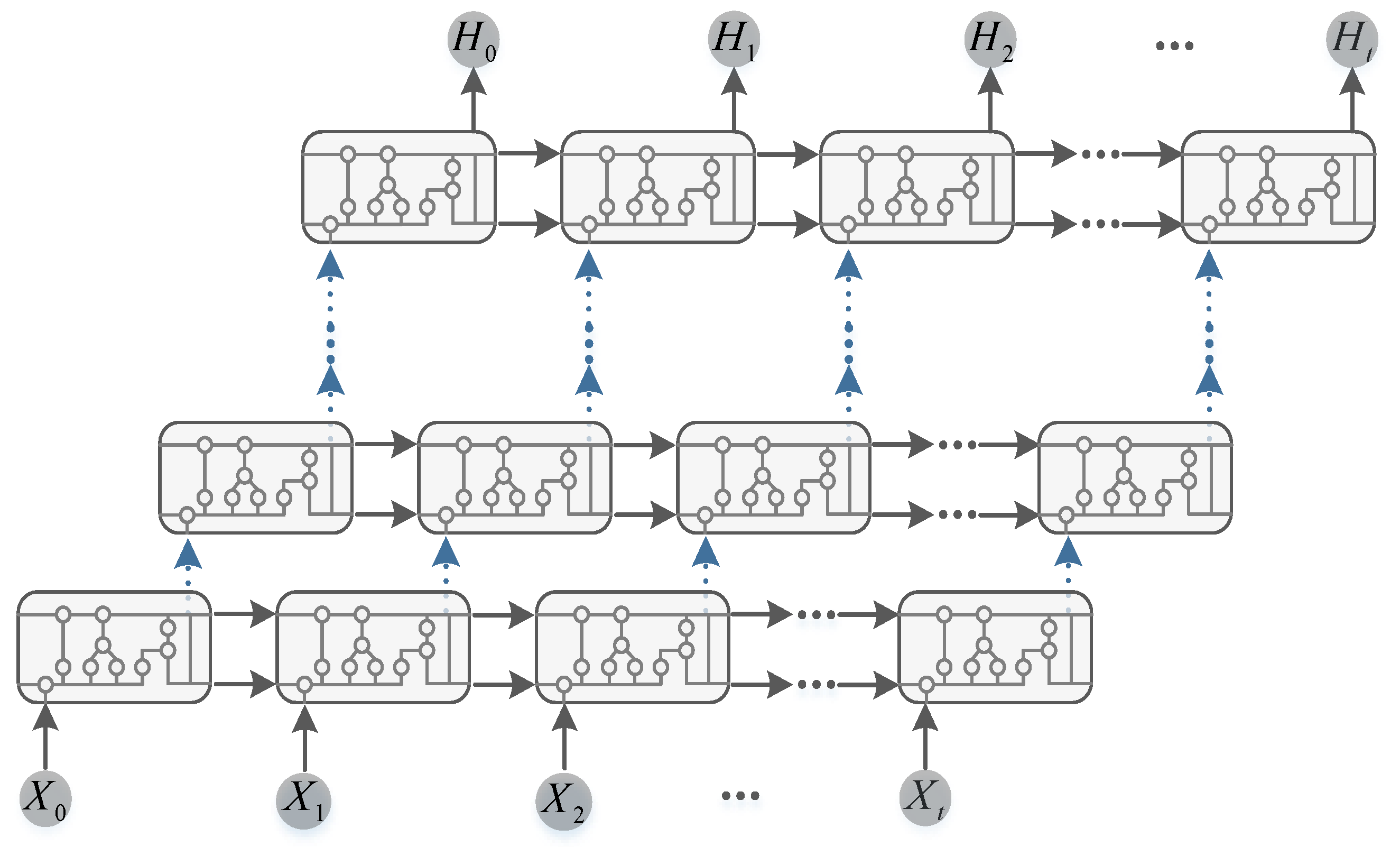
is a non-linear transformation that multiplexes the effective features of the network front-end to enhance the propagation of data through the network. Since the input dimension of the LSTM has to be the same as the number of hidden neurons, the data dimension is reset, the number of hidden neurons of the LSTM is 40, and the deep LSTM is set to two layers. Finally, the mixed load features are input into five branches, and the predicted power values of the target appliance are output through the fully connected layer. The Long and Short Time Memory Multiple Output Network proposed in this section is mainly intended to solve the disadvantages of a high computational cost, a large number of parameters, and a poor overall decomposition of the model, reflecting the more excellent generalization performance of the M-LSTM. The deep LSTM structure is constructed on the basis of the LSTM cycle unit. The deep LSTM structure will be copied many times at the same time. By using the cyclic unit structure, the network model can enhance its ability to extract and express the load time series information and capture the deeper dependence of the load characteristic time series information so as to effectively enhance the decomposition performance of the network model and the identification effect of the load operation state.
Figure 2 shows the time step expansion structure of the deep LSTM structure, and each small part represents an LSTM cycle structure so as to learn the load data patterns and make the network model have a good decomposition effect.
To address the drawback that traditional convolutional neural networks do not sufficiently extract load features and to enhance the generalization ability of long- and short-term memory multi-output networks for better non-invasive load decomposition tasks, this section proposes a multi-scale fusion residual module (SRM) as a pre-activation module for features. Due to the deepening of the layers of the neural network model, it is basically difficult to generate parameter perturbations when the errors are back-propagated to the previous layers, resulting in the parameters of the layers not being updated, which causes the problem of the network having a difficult time learning from the training data.
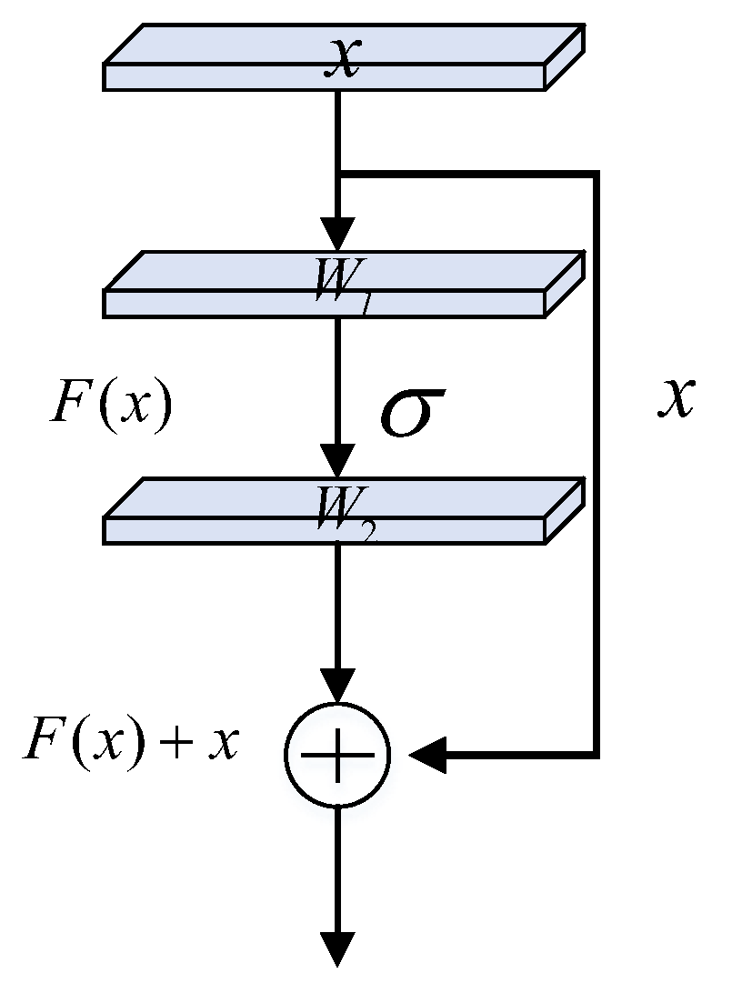
The residual convolutional neural network (Resnet) is a good remedy for gradient dispersion and the degradation of performance due to the deepening of the network. The residual convolutional neural network is based on the idea of “cross-layer connection”, through which the original input feature mapping and the output feature mapping of the later layer are added together and activated by the activation function to complete the fusion of the features, and the residual connection makes the backward and forward information transfer of the network smoother.
Figure 3 shows how the residual structure is connected. Define the underlying mapping as
H(
x) by using the stacked layers to fit
F(
x) =
H(
x) −
x and add the input of the residual
unit to obtain the output of the residual unit
F(
x)—that is, the residual function.
In the underlying structure of the residual connection, the residual connection mainly consists of two weight layers, each of which contains weight parameters.
denotes the input. The expression of the residual connection is as in Equation (2), where
denotes the Relu nonlinear activation function.
Finally, the input is passed
through a cross-layer connection, and the output of the second weighting layer is added to obtain the final output of the whole residual structure. The calculation formula is as in Equation (3).
where
is the residual mapping function that is to be trained to learn in residual connectivity, and
is the set of weight matrices. We can obtain Equation (4) based on Equations (2) and (3).
where
is the output feature mapping of the
L-th residual connection in the residual structure, and
is the input feature mapping of the
L-th residual connection in the residual structure. From this, it can be deduced that the output feature mapping of the
L-th residual unit can be decomposed into the sum of the input feature mapping of the
L-th residual unit and the feature mapping between the two residual connections. According to Equation (5), it is known that the gradient of the neural network does not converge to 0 during back propagation.
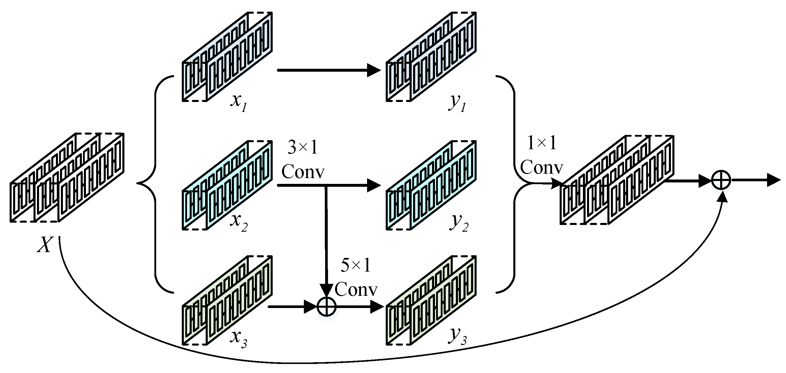
Based on the residual connection, this section proposes a multiscale fusion residual module for the network model to extract the base load features [
28], using the features of different resolutions to improve the multiscale capability of the load and allow the network to have more perceptual fields, with the structure shown in
Figure 4.
The multiscale fusion residual module adjusts the number of channels by convolving the original feature map three times, with 40 convolution kernels, and divides the feature map into feature map1 (in the figure ), feature map2 (in the figure ), and feature map3 (in the figure ). In the first part, feature map1 is directly passed to without any operation; in the second part, feature map2 is convolved, the number of convolution kernels is 40, and the feature map is directly passed to ; in the third part, there is another role, a tensor sum operation with feature map3, which is then convolved, the number of convolution kernels is still 40, and the result is obtained. The feature maps , , , containing different scales, are fused and then convolved to output.
The stacked multi-scale fusion residual module enhances the extraction of complex features of residential household electricity data, preserves the main features of the time-series information, and improves the ability of the network model to fit the load features, while ensuring that the error signal can be continuously transmitted during the back propagation [
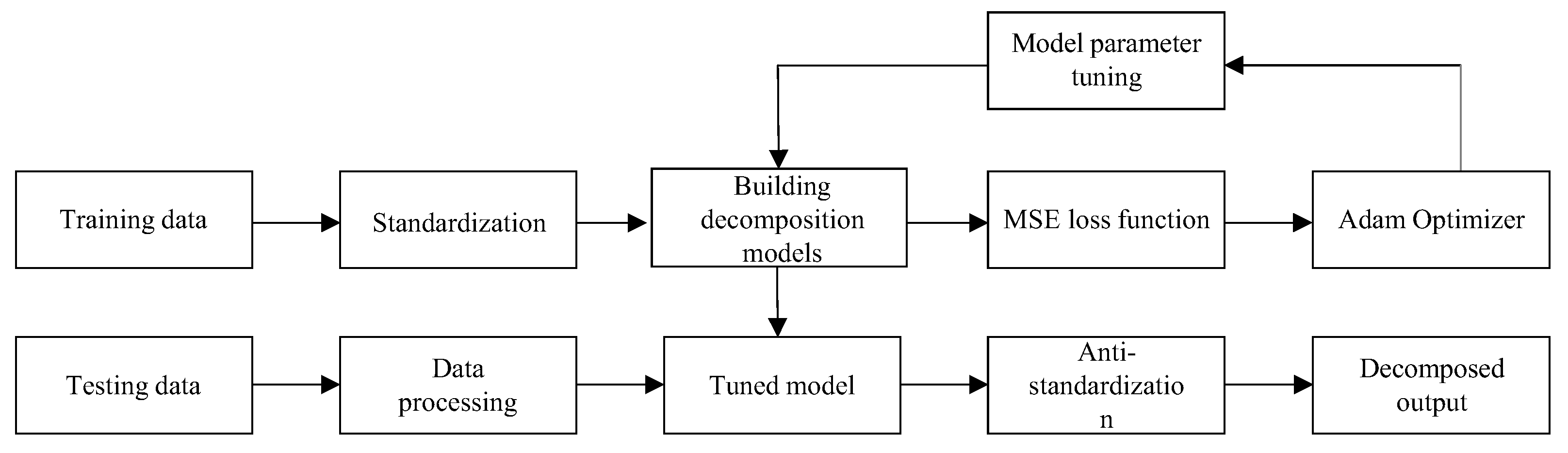
29]. The overall algorithmic flow of the network model is shown in
Figure 5, including the selection of the load device, the division of data samples, the method of data pre-processing, the construction of the model, the training of the model, and the tuning of the model.
To better train the multilayer neural network, the BP algorithm, i.e., the error back propagation algorithm, is used, the pre-processed data samples are passed through the neural network one by one to calculate the weighted sum of the neurons of each layer, and then the result of the activation calculation using the nonlinear activation function of each layer is used as the input of the neurons of the next layer, and this process is repeated at each network layer to obtain the forward propagation calculation result [
30,
31]. In this paper, we use the mean square loss function, i.e.,
, calculate the difference between the computation result of the last layer of the network and the target load power value, and this obtained error value is passed in a backward propagation way to calculate the difference of the previous layers separately, using the adaptive moment estimation optimizer Adam to adjust the parameters of the neurons in each layer to make them optimal, which is a complete learning process [
32]. The specific process is shown below.
The input matrix of the next network layer of the model is calculated using the forward propagation calculation method [
33,
34]. This is shown in Equation (6).
where
represents the input matrix
of the layer neuron,
represents the weight parameter matrix from layer
to layer
,
represents the nonlinear activation function of the layer, and
represents the bias parameter
from layer to layer. Assuming that the input value of the first layer
is represented by a vector
, then the final output value of the first
layer in the neural network is
, as shown as in Equation (7).
where
and
still represent all the weight parameter matrices and bias parameters in the neural network. Finally, the difference in the neurons in each layer of the neural network is calculated by back propagation, and this difference is used to adjust the optimization network, as in Equation (8).
where
denotes the tensor dot product operation,
denotes the
layer error value matrix, which is calculated from the error values of the
layer, and the whole process above represents the error back propagation. The following is the process of updating the parameters of the optimizer Adam, as shown in Equations (9)–(13).
where
denotes the learning rate,
,
denotes the exponential decay rate when the neural network performs moment estimation, and the initial condition is
,
.
3. Results
3.1. Dataset Introduction and Appliance Selection
The model-based load decomposition methods need some high-quality power datasets to evaluate the decomposition performance of these methods in the process of practical application. The Wikienergy dataset is a research power dataset released by the Pecan Street company. It is the most abundant residential power energy database studying power load decomposition in the world. It contains the power data collected by nearly 600 household users over a period, including single load and total household power consumption. All loads and residential active power are obtained at the sampling frequency of 1/60 Hz. The collection of power data began in 2011, but it has not stopped. The database is still expanding, which provides good data support for the research of non-invasive load decomposition. The UK-DALE public dataset [
27] was collected and released by the British scholar Kelly. The dataset mainly contains the information of single load and total household power consumption in five household users. There are up to nine load devices in each household, but the sampling period of each household is different. Here, the active power data collected at a 1/6 Hz sampling frequency is mainly used. The two datasets in the article are the data obtained from practical applications and have corresponding labels. The two test datasets used in this paper are the standard datasets in the field of non-intrusive load disaggregation, which have very good practicality because these two data sets are collected by actual resident families.
The NILMTK toolkit is used to extract five kinds of load appliances from Wikienergy metadata as research objects: air conditioner, refrigerator, microwave oven, washing machine, and dishwasher. Five kinds of loads are extracted from UK-DALE metadata as research objects: kettle, refrigerator, microwave oven, washing machine, and dishwasher. The main reasons for choosing these loads are: (1) these loads exist in multiple families, which means that the load data can contain some similar load changes, which has a better generalization for the training of a network model. (2) There are many kinds of loads in a family, and these loads have different load characteristics and different work cycles. It is not necessary to experiment each load that has a large number of tasks and a high time cost. (3) There are some loads with low power in the family, such as the mobile phone charger, which is easily interfered with by other signals, so it is difficult to decompose, and the power of the overall power consumption data can be ignored, so the research on this kind of electrical appliances is not done. (4) These kinds of loads have accounted for most of the energy in the family, which means that the results of the load decomposition are of certain significance to the energy conservation and consumption reduction of the family. Therefore, the selection of these loads can meet the research purpose of this paper.
3.2. Data Preprocessing
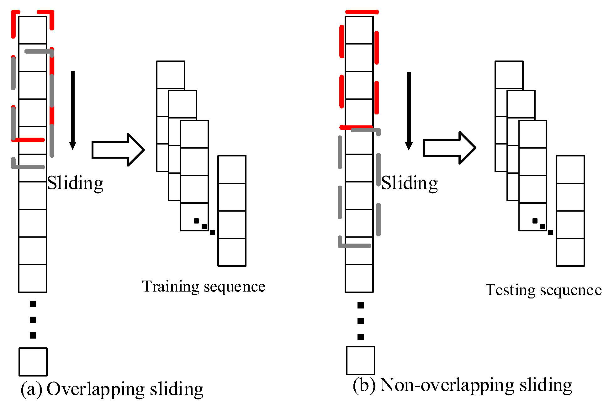
A neural network needs a large number of training samples to fine tune in order to exhibit good performance. In addition, before the data are input into the neural network, they must be transformed into a consistent input dimension, and each piece of data is segmented into a vector of identical length, which is called a window. Therefore, the training sequence and test sequence are sliding processed.
As shown in
Figure 6a, the data are added by overlapping sliding for the sliding window of the training sequence. Assuming that the sequence length is M, cut a window with length N on the original data, and the sliding step is 1, and then conduct the sliding operation to obtain M – N + 1 training samples. Similarly, as shown in
Figure 6b, H/N test samples can be obtained by using the non-sliding window method on the test sequence and assuming that the sequence length is H.
After synthesizing all the data, this paper divides them into a training set and test set for better training and more accurate evaluation. In this work, the data input we use is the total power of electricity, and the output is the decomposition power of each electrical appliance. Take 80% of the data as the training sequence and the remaining 20% as the test sequence. When the input data are close to the “0” average value, the learning efficiency of the deep learning algorithm is the highest. In order to eliminate the impact of the index dimension and numerical range on the experiment, the data are standardized. Common methods include Max-Min Standardization, Z-score standardization, and Nonlinear Scaling. In this paper Max-Min Standardization is used, and the data are mapped between [0, 1]. The standardized function is shown in Equation (14).
where
is the consumption power of the unstandardized target load at time
,
is the maximum value of the total power sequence,
is the minimum value of the total power sequence, and
is the standardization result at time
.
3.3. Experimental Indicators
In this paper, mean absolute error (MAE) and signal aggregate error (SAE) will be used as evaluation indexes to analyze the effect of load decomposition. MAE is mainly used to measure the average error between the power of the single load equipment decomposed at each time and the real power, which reflects the instantaneous load decomposition ability of the decomposition model. However, for some load equipment, the error at each time point is not obvious and important, so it is only interested in the error of total power in a long time. SAE is used to measure the error of total energy consumption of each family in the whole time period.
In addition, when the load is decomposed, the on/off state of load equipment is distinguished by thresholding, and the load decomposition task is transformed into the load identification task. In order to judge the switching state of the load, first set the power threshold as follows: kettle 2000 W, air conditioner 100 W, refrigerator 50 W, microwave oven 200 W, washing machine 20 W, and dishwasher 10 W. Recall, precision, accuracy, and F1 values are used to evaluate whether the load decomposition model correctly classifies the switching state of the load in order to judge the decomposition performance.
3.4. Analysis of Experimental Results for the WikiEnergy Dataset
Experiments were conducted on the WikiEnergy dataset household 25, where several representative load devices—namely, air fade, refrigerator, microwave, washing machine, and dishwasher—were selected for analysis. The built network model is based on the Keras deep learning framework with an RTX1060 6g video memory discrete graphics card and is based on the adaptive matrix optimizer (Adam) when training the network model, where the superparametric learning rate is set to 0.001 and the weight decay rate is 0.0005.
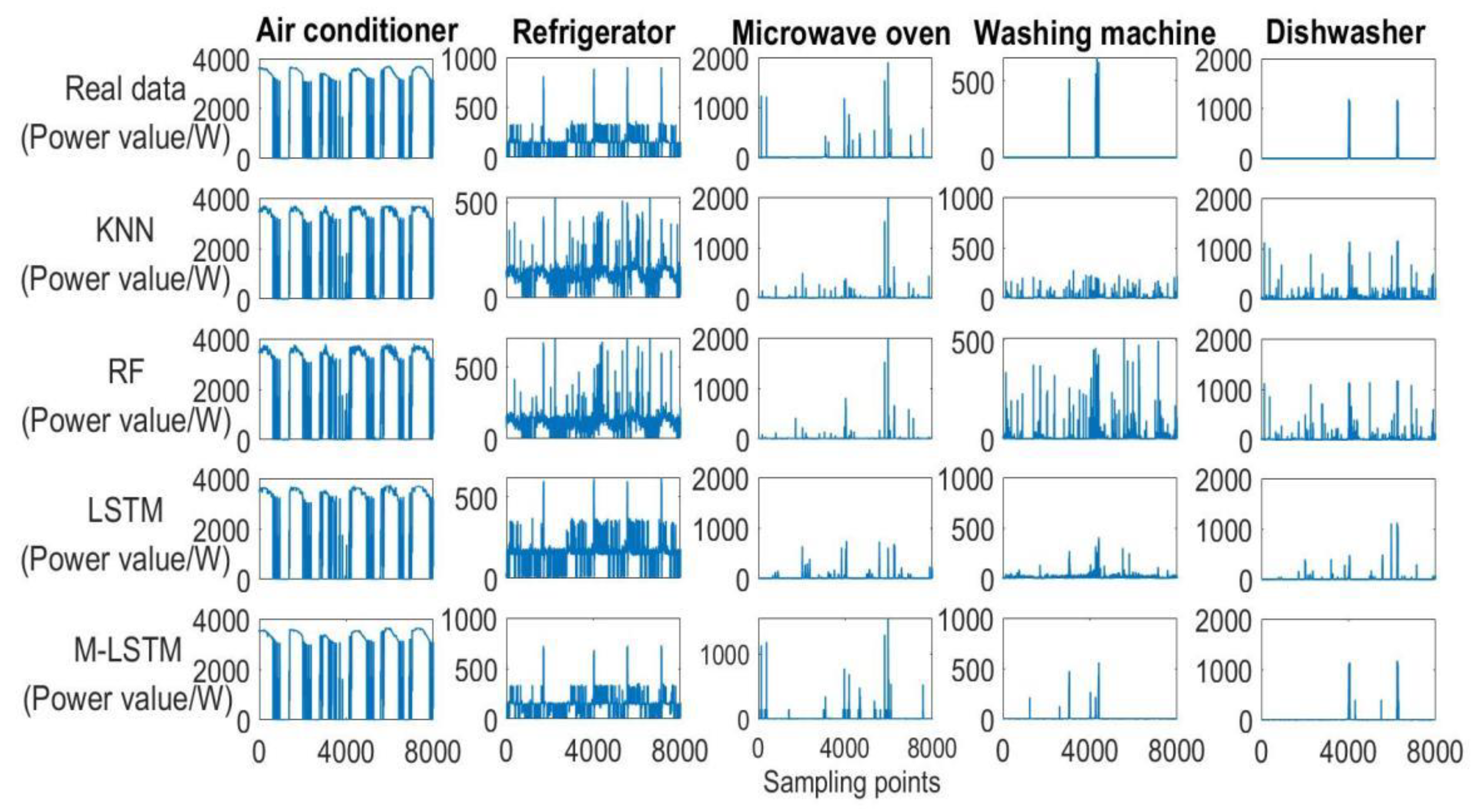
During the experiments on this dataset, we used three methods for comparison experiments with this method, which are the classical KNN algorithm, Random Forest (RF) algorithm, and deep long- and short-term memory network (LSTM), which are used because the KNN algorithm is the more commonly used method in non-intrusive load decomposition. To better reflect the performance of this section algorithm’s generalization performance, Random Forest and LSTM are brought in to compare with it. The experimental results of the load decomposition are shown in
Figure 7. On the loads with more sufficient data samples, such as air conditioners, refrigerators, and microwave ovens, KNN, Random Forest, LSTM, and the M-LSTM proposed in this paper have good decomposition results, especially the M-LSTM model, for which the fitted curve is closer to the real power data curve. However, the decomposition is even less effective than the methods in this section with respect to underutilized appliances such as washing machines and dishwashers.
From
Figure 7, it was found that the decomposition results of the comparison algorithms were very similar for some loads, and it was difficult to distinguish the differences in the algorithm decomposition performance, so a large number of reliability assessment metrics were chosen for the evaluation.
Table 1 shows the results of the WikiEnergy 25 home load decomposition evaluation metrics comparison, using the mean absolute error and the combined absolute error for evaluation and analysis. As can be seen from
Table 1, the LSTM model has a more obvious decomposition advantage in MAE and SAE when comparing the KNN algorithm and Random Forest, an integrated learning algorithm, but the M-LSTM model proposed in this work uses the multi-scale fusion residual module to enhance the extraction capability of the base load features, so it can perform better than the simple stacked LSTM model in achieving an accurate decomposition of the total energy.
To demonstrate the superiority of the model proposed in this work, the operating state of the load equipment is used to judge the effectiveness of the algorithm in identifying individual loads. The operating state of the load is judged and identified by setting the threshold value of the start-stop state of the device and converting the power value into the actual switching state.
Table 2 shows the comparison of the operating states of the WikiEnergy 25 home loads. Based on the three metrics of Precision, Accuracy, and F1 value, the method in this work achieves more accurate prediction results regarding the operating status of all five types of load appliances: air conditioners, refrigerators, microwave ovens, washing machines, and dishwashers. As a whole, the KNN algorithm and Random Forest algorithm do not differ much in each evaluation index, indicating that the simple algorithmic model can only obtain rough decomposition results.
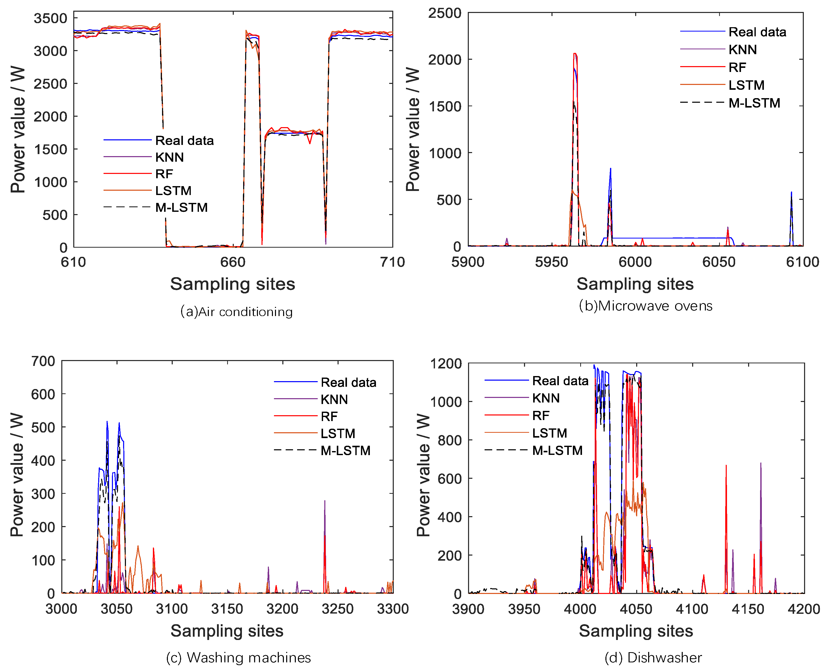
To be able to observe the decomposition effect in specific detail, the analysis was performed using the load local decomposition effect graph. As shown in
Figure 8, a comparison of the local effects of each algorithm on each load device is shown, with the horizontal coordinates representing the sampling point interval.
Figure 7 shows that the M-LSTM model has a better algorithm performance and can fit the actual power curve better compared to other models. While the KNN algorithm and Random Forest algorithm have a poorer fitting ability for load devices with sparser features, the M-LSTM model still fits the power curves of washing machines and dishwashers well to some extent.
3.5. Analysis of Experimental Results for the UK-DALE Dataset
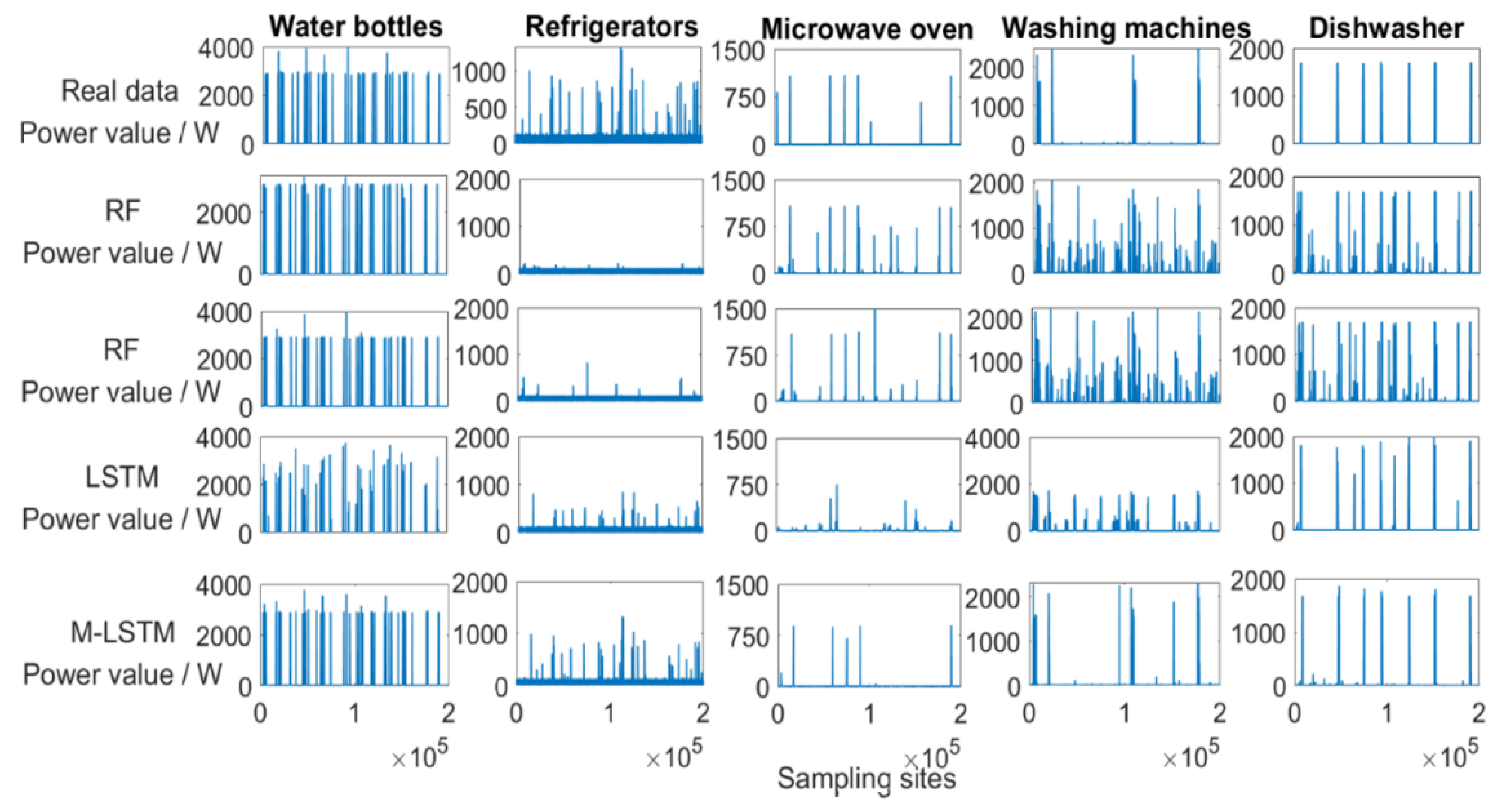
To verify the generalization performance of the model in this work, relevant comparison experiments were conducted on the UK-DALE 5 household. The five loads—kettle, fridge, microwave, washing machine, and dishwasher—were selected for the analysis of this household. The decomposition effect of the test set is shown in
Figure 9. As can be seen from the figure, KNN, Random Forest, LSTM, and the method in this work all achieve good results for this high-powered load refrigerator, but the decomposition on the microwave, washing machine, and dishwasher is indeed not as effective as that of the improved method proposed in this work.
Table 3 shows the comparison of the load decomposition assessment metrics for the methods in this work for UK-DALE 5 households. From
Table 3, it can be seen that, in the MAE metric, the M-LSTM model has the smallest value compared to the other algorithms on the load devices of kettle, washing machine, and dishwasher. In the other evaluation metric, SAE, the KNN algorithm performs the best on the appliance microwave oven, and the LSTM model is poorer. Combining the MAE and SAE metrics, it is feasible to apply the M-LSTM model to the task of non-intrusive load decomposition.
Table 4 provides a comparison of the evaluation metrics for different loads in UK-DALE 5 households in terms of switch operation status recognition. From several of these evaluation metrics, the M-LSTM model proposed in this work has a better recognition performance. The KNN algorithm is relatively simple but still identifies the start-stop state of the kettle and the refrigerator. From the four evaluations metrics, the random forest algorithm and the LSTM algorithm have a weaker load feature extraction and therefore perform poorly on the switch judgement. In this work, the network structure is improved, and the decomposition ability of the model is effectively improved by using multi-scale fusion residual blocks to extract the base load features and deep LSTM cyclic units in order to learn the timing information. Combining
Table 3 and
Table 4, the M-LSTM model has a higher decomposition accuracy than the ordinary LSTM model in the UK-DALE dataset.
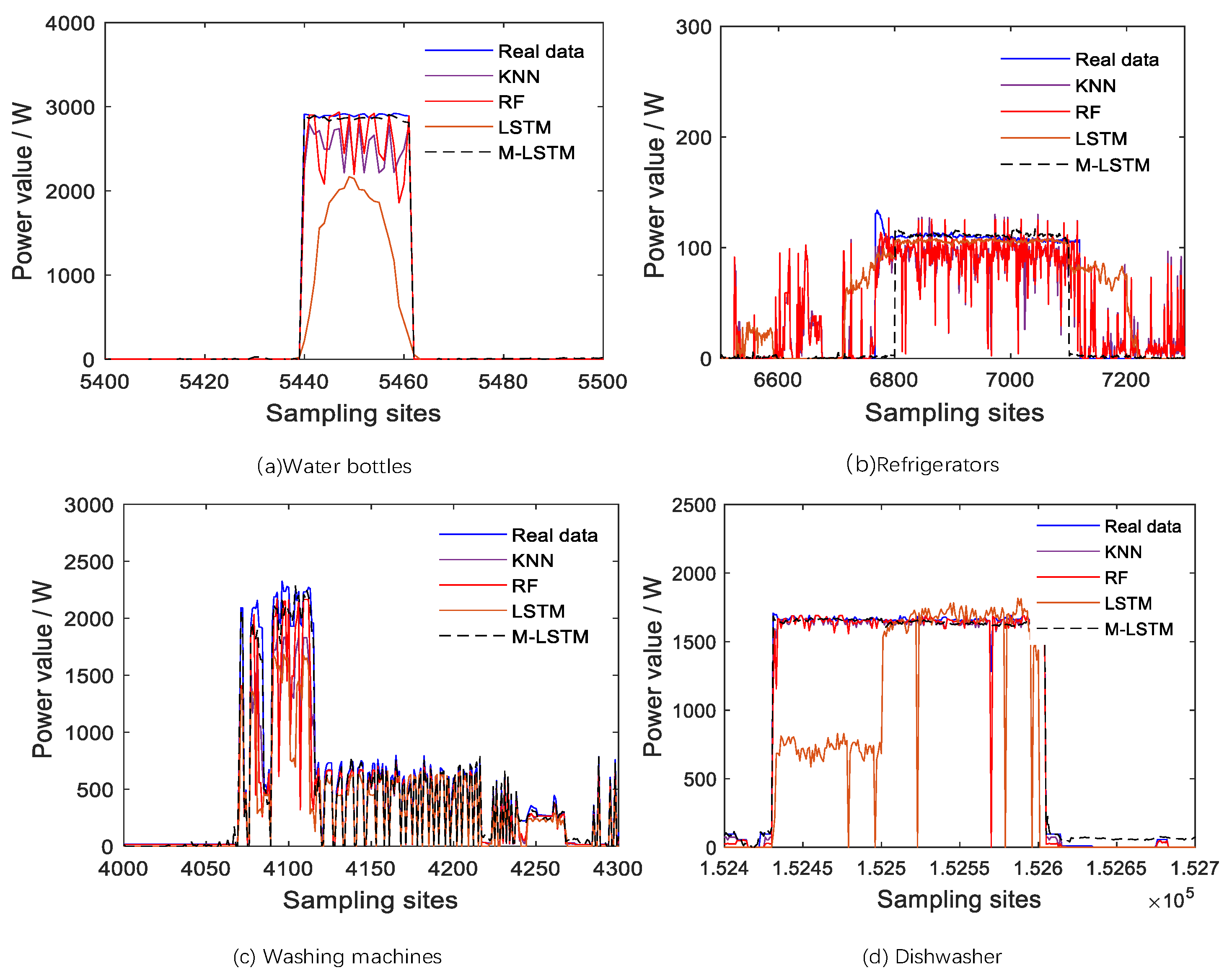
Meanwhile, the local decomposition effect graph of the load device is selected for analysis. From
Figure 9, it can be seen that the decomposition ability of the M-LSTM model is better than the other algorithms, and the power curve is the closest to the curve of the real data. Looking at these detailed decomposition effect plots, the KNN model’s decomposition results have large burrs on multiple devices, and the overall tracking trend is not too good, while the random forest algorithm’s decomposition is found to fluctuate too much in the local decomposition plots of the refrigerator. It can also be seen from
Figure 10 that the decomposition results of the LSTM method are very stable and outperform the KNN model and Random Forest model, but the decomposition performance remains weaker than that of the M-LSTM model proposed in this work because of the simplicity of the model and the inadequate feature extraction.


 and
and 


