
Scale Model Experiments and Simulations to Investigate the Effect of Vehicular Blockage on Backlayering Length in Tunnel Fire

 , ,
, ,
Abstract
:1. Introduction
2. Model Tunnel and Experimental Procedure
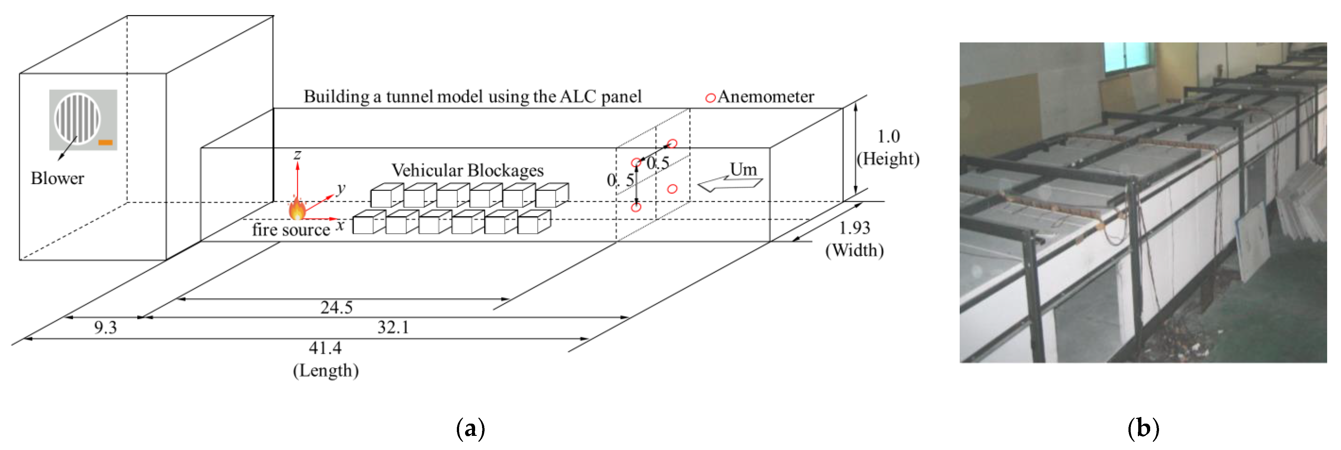
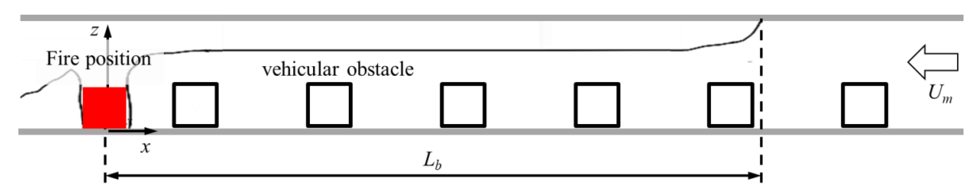
2.1. Scale Model Tunnel
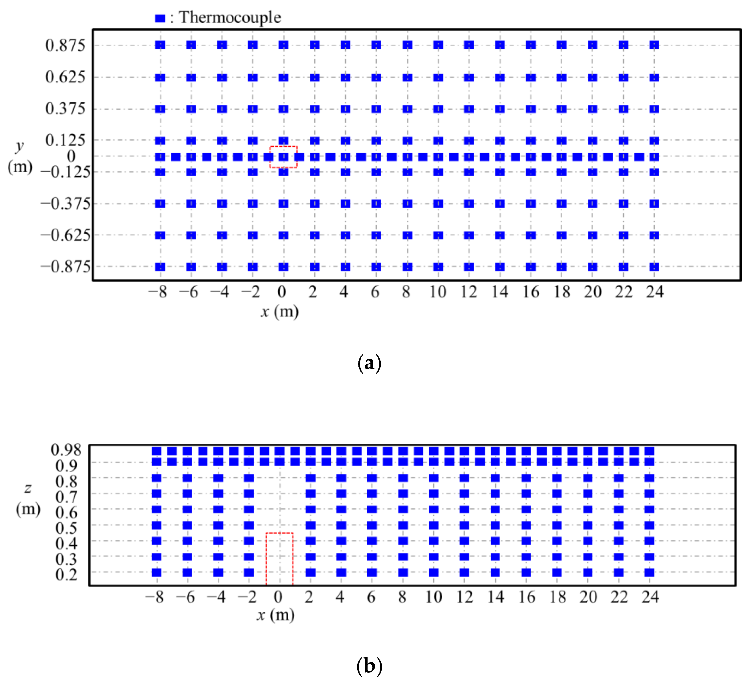
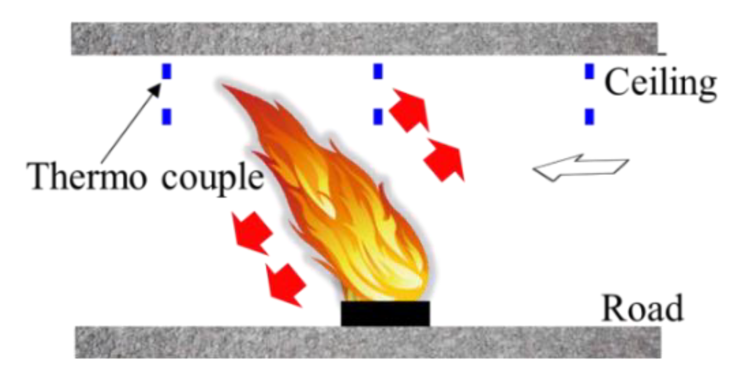
2.2. Temperature and Smoke Measurement System
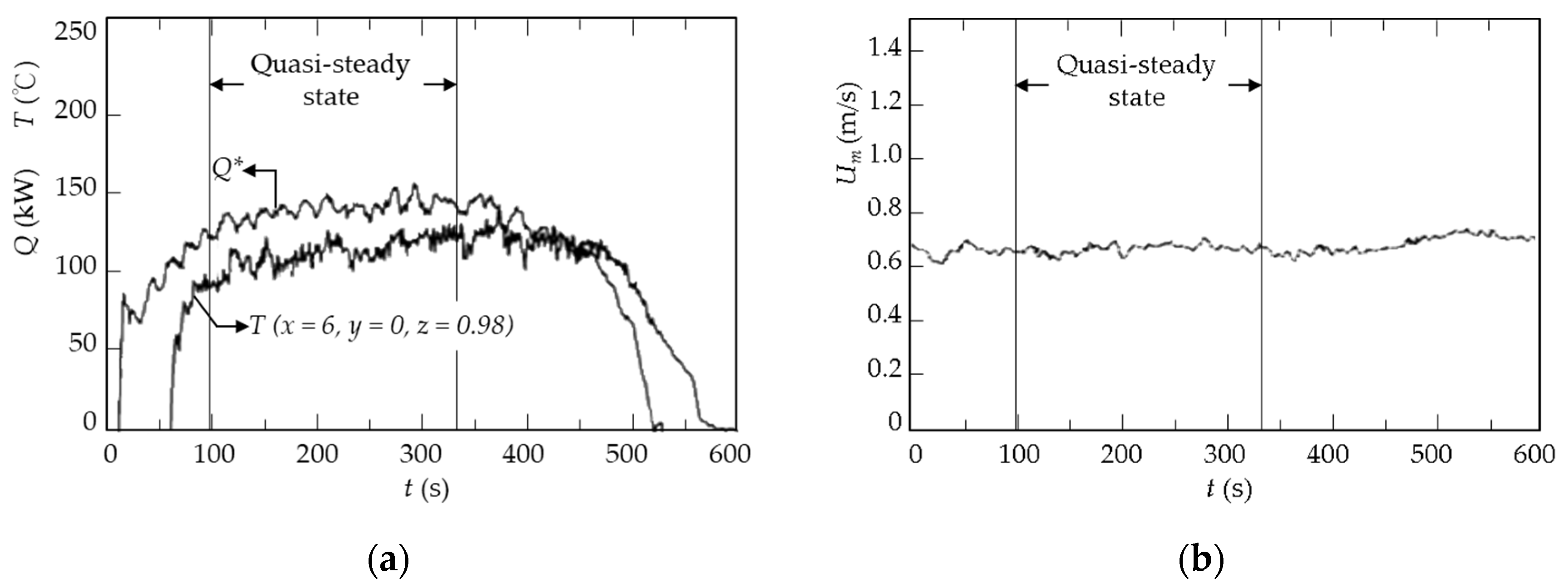
2.3. Heat Release Rates
3. Investigating the Effects of the Configuration and Height of Vehicular Blockages
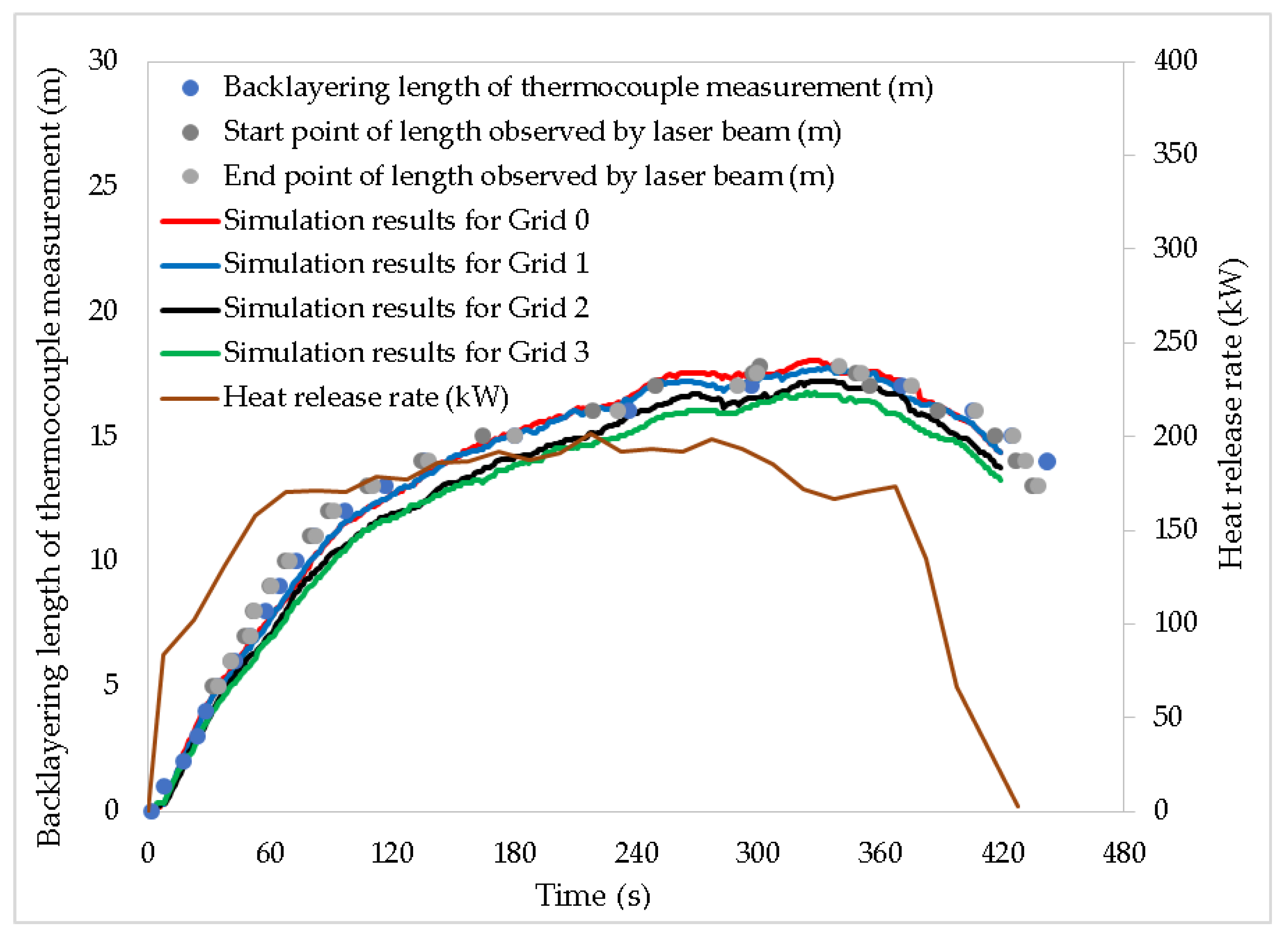
3.1. Simulatior and Verification of the Grid Size
- (i)
- The laminar boundary layer.
- (ii)
- The wall function for a smooth wall involving in the turbulent boundary layer.
- (iii)
- The same as the surface roughness.
- (i)
- h is a constant.
- (ii)
- The Yurges formula:
- (iii)
- Colburn’s analogy.
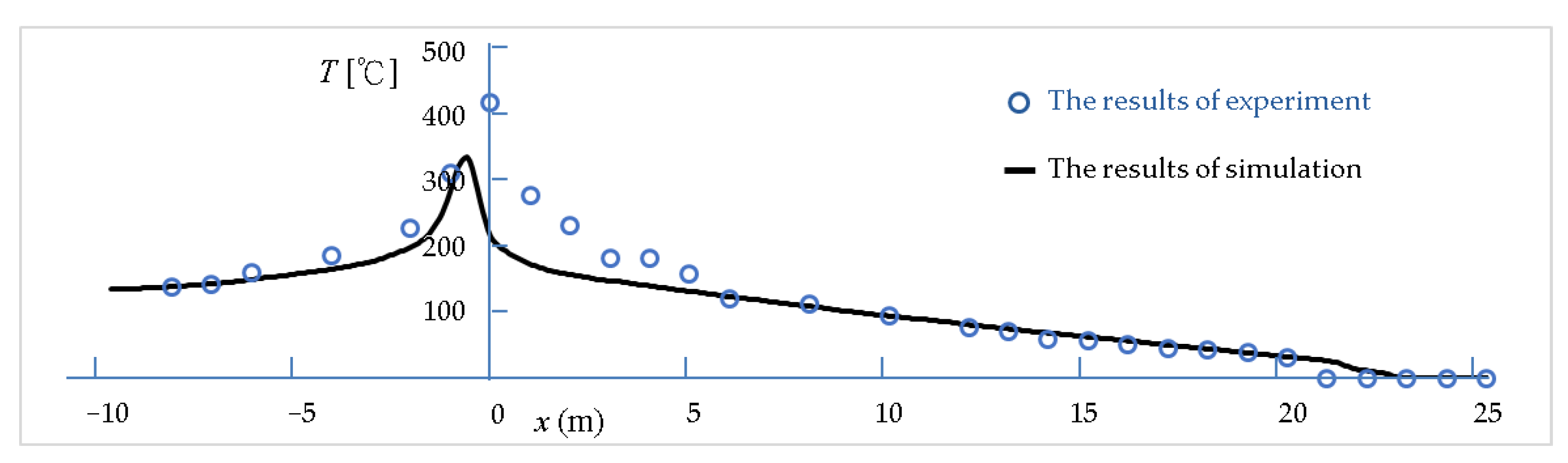
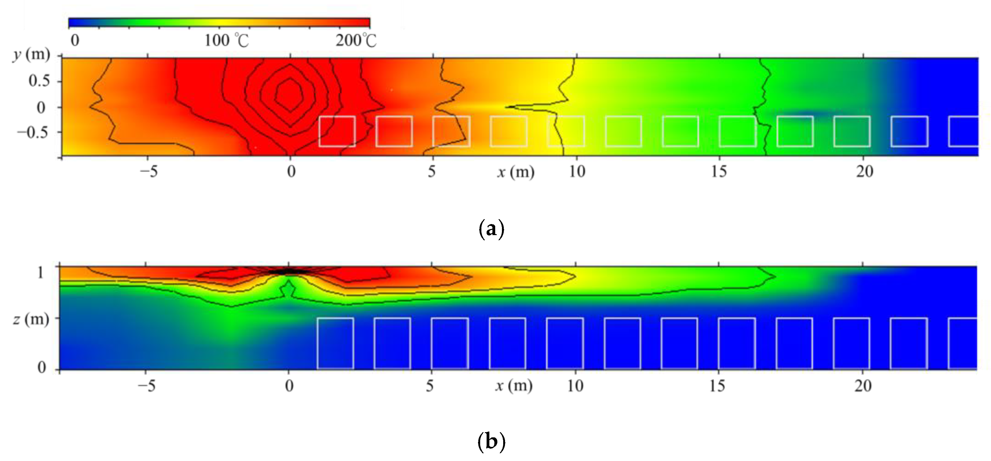
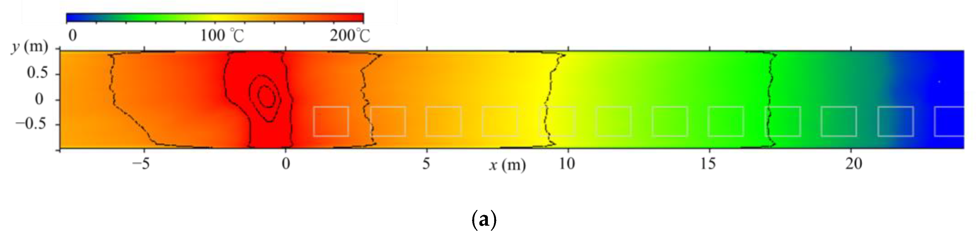
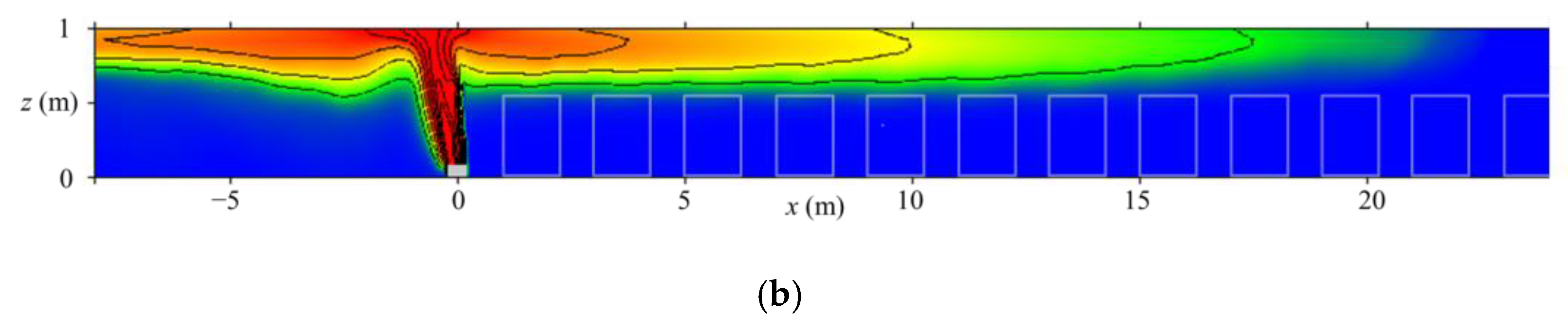
3.2. Comparison of the Experimental Results and Simulation Results
3.3. Comparing the Effects of the Configuration and Height of Vehicle Blockage
4. The effect of Vehicle Blockage Ratio on Backlayering Characteristics
4.1. Li et al.’s Empirical Equation of Backlayering Length
4.2. Comparison and Discussion of Pattern A and Pattern B
4.3. Verification and Discussion of the Approximation Formula
5. Conclusions
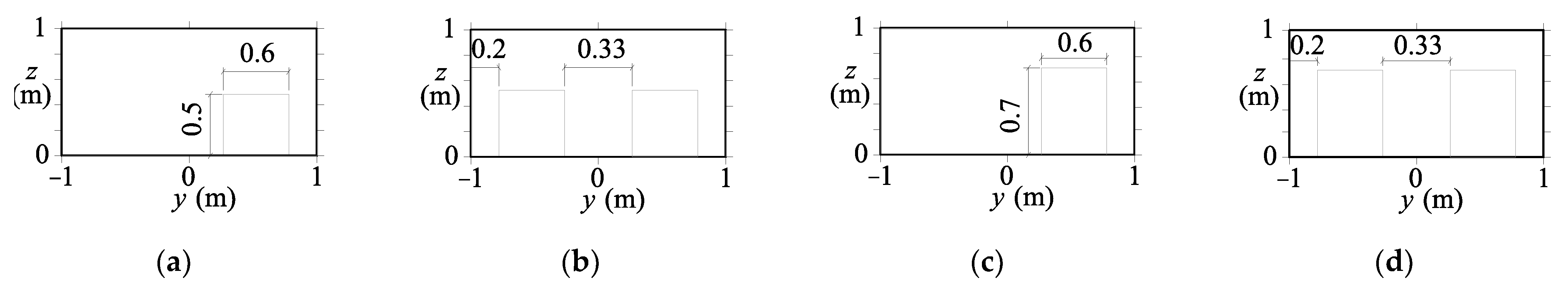
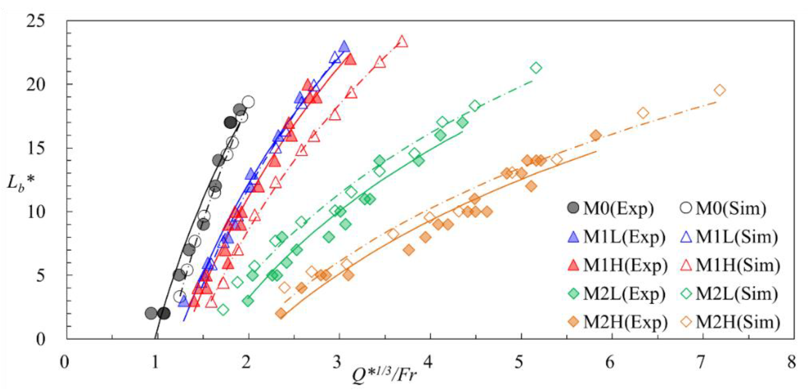
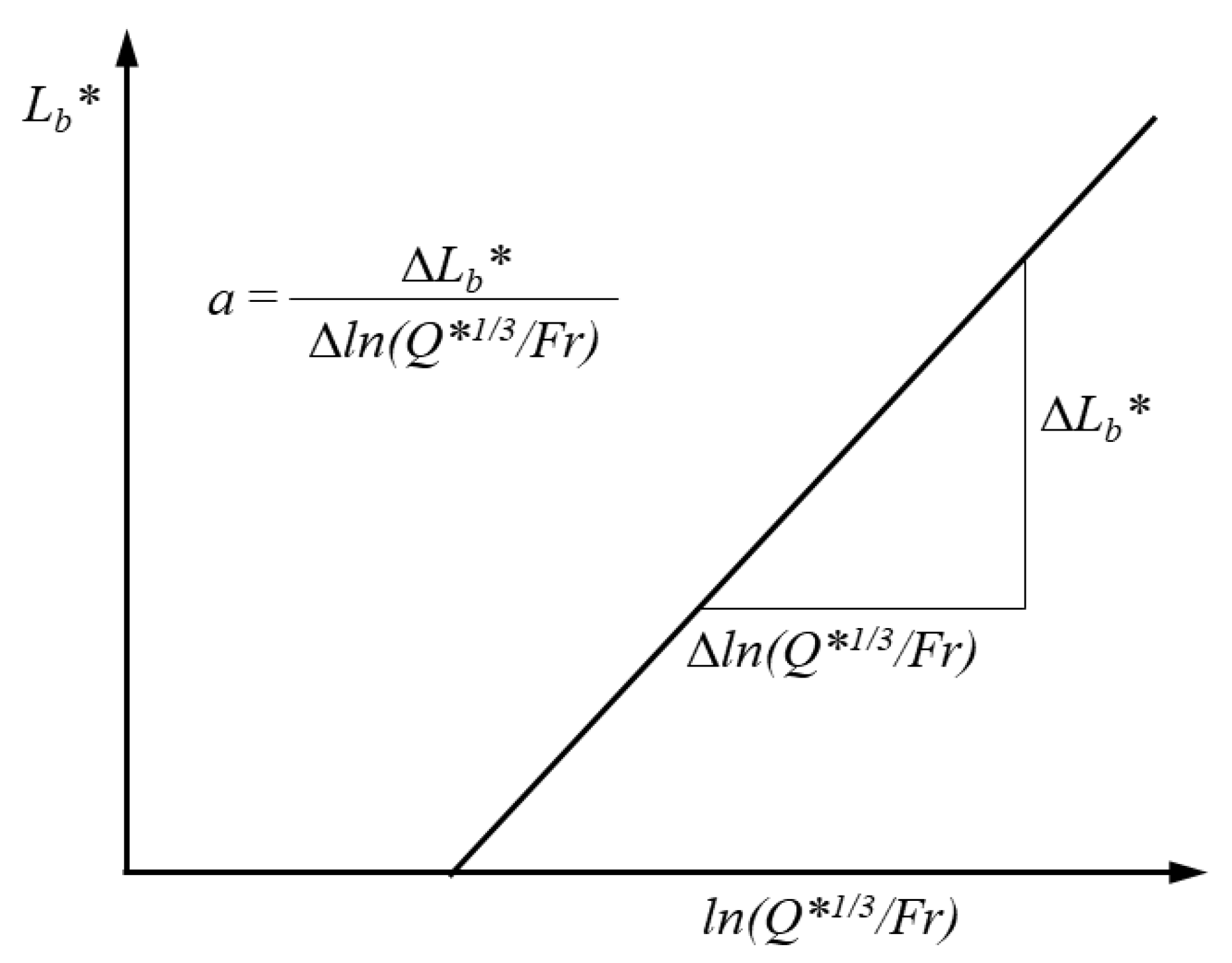
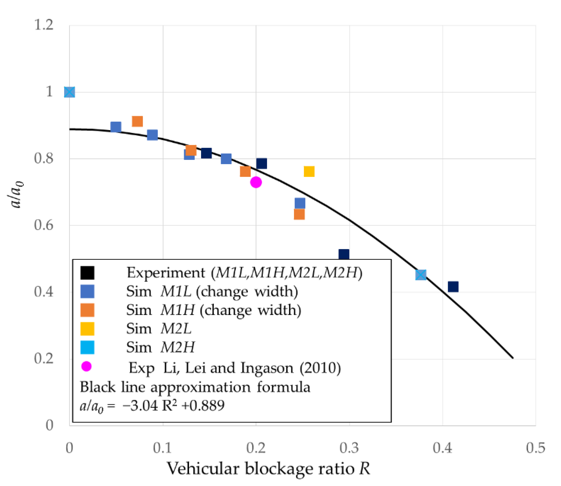
- According to the results, if there were vehicles on one side of Lane 1 (M1L and M1H), the height of the obstacle had little effect on the backlayering length extension rate a. Compared with the situation where there were vehicles on one side of Lane 1, when there were vehicles on both sides of the lane (M2L and M2H), a was significantly reduced. In addition, in the case of M2H, a had the greatest decrease. It was reduced to about 52% of a0 when there was no vehicle with a vehicle height of 2.62 m in M2L and to about 44% of a0 with a vehicle height of 3.57 m in M2H.
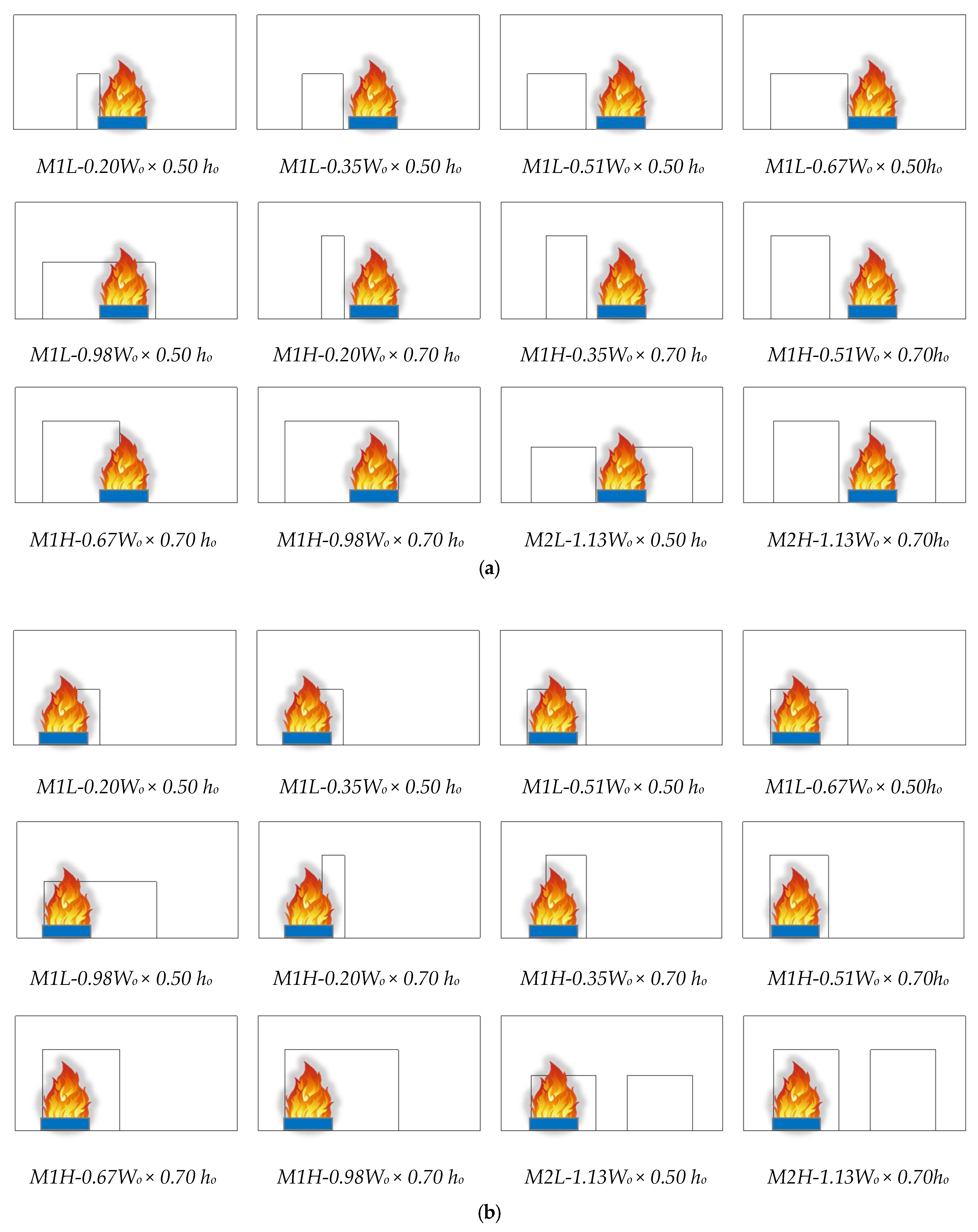
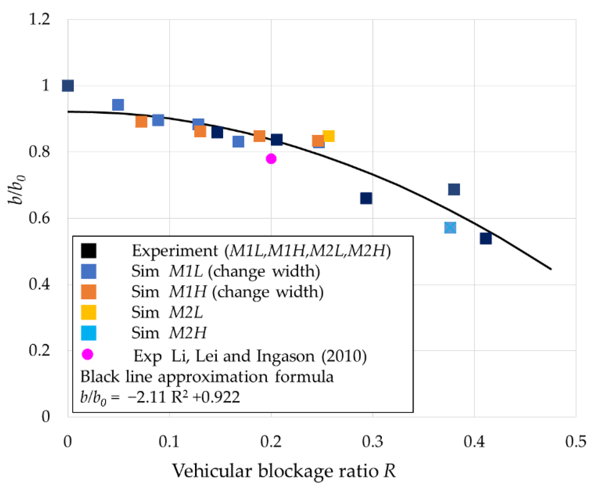
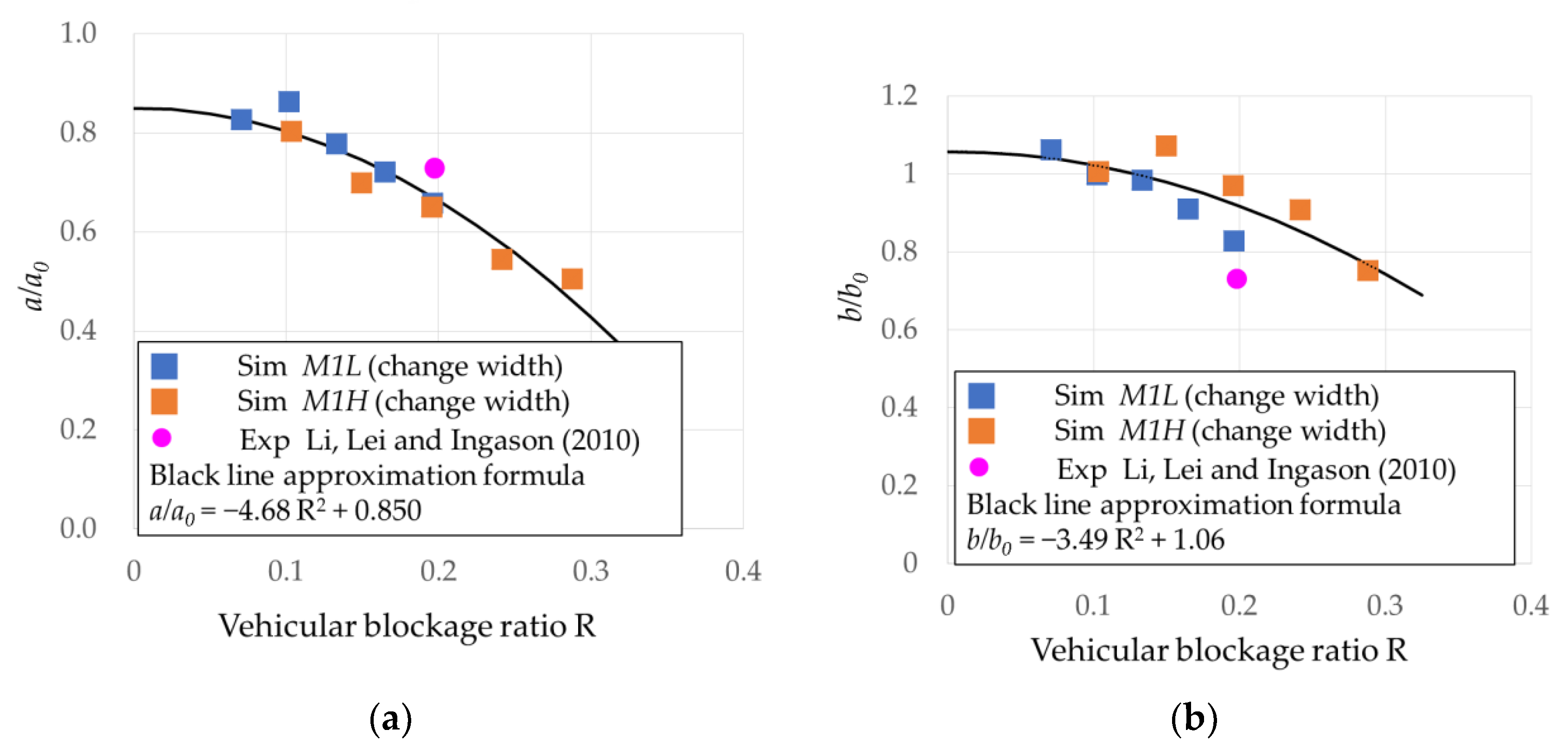
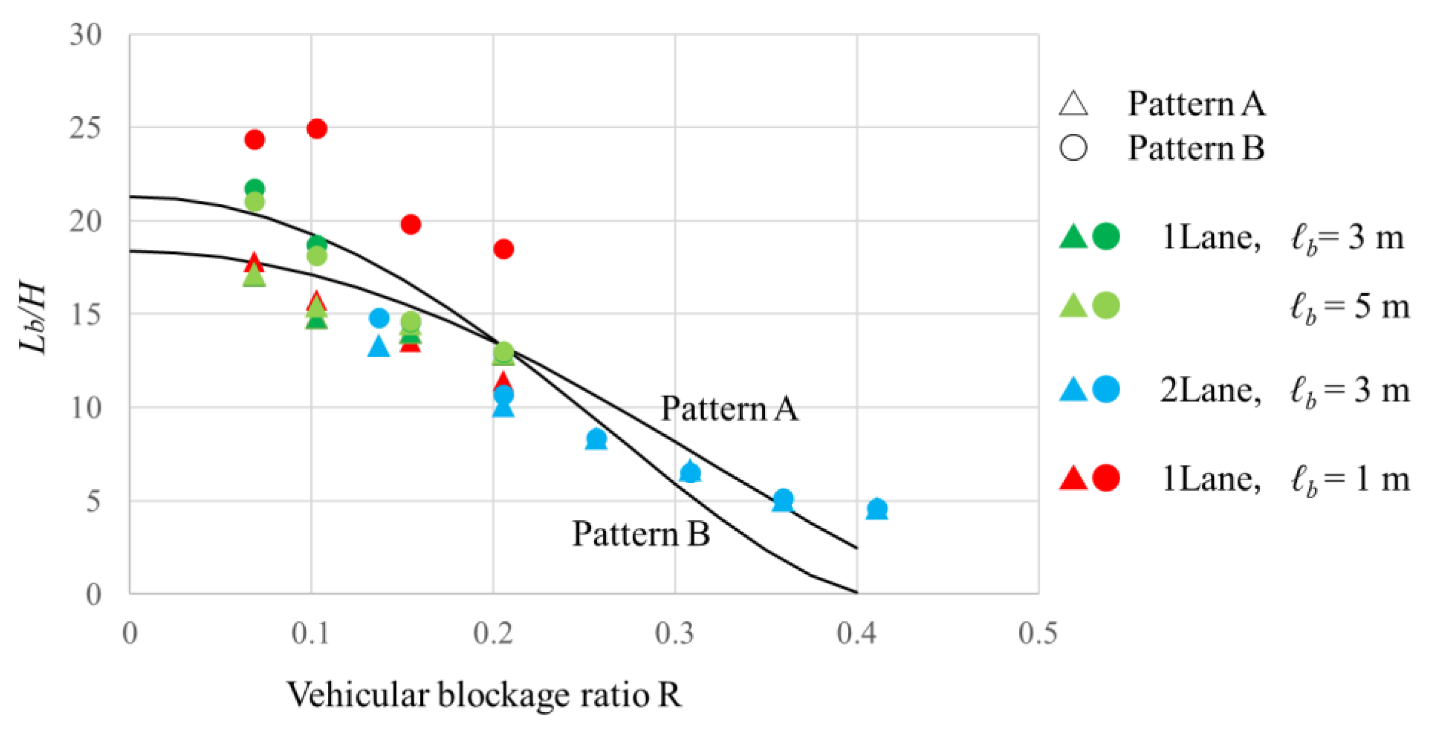
- In the configuration of Pattern A, when R < 0.2 was in the low blocking rate domain, the experimental and simulated results were consistent. Even if R > 0.2, there was no significant deviation. In addition, the rectangular tunnel section used in this study was the same as the semicircular tunnel section used in previous studies. With the configuration of Pattern B, the approximation formulae were coincident with each other in the range of R < 0.2. Although slight deviation could be observed in R > 0.2, in reality, the vehicular blockage ratio R of one large vehicle was only about 0.15–0.2.
- Nearly all backlayering lengths with obstacles could be approximated by the approximation formula of Pattern A. If the blockage ratio was lower than 0.1 when a single lane had an obstacle, the approximation formula of Pattern B was applicable. However, when the fire source was close to the obstacle, the fire plume was pulled to the obstacle through this reflux region and the backlayering length became unstable, and it could not be represented by the approximation formula of this study.
- When the distance between stationary vehicles on the upstream side of the fire source was small, the backlayering length may have been longer than in the case with no vehicular blockage.
Author Contributions
Funding
Institutional Review Board Statement
Informed Consent Statement
Data Availability Statement
Acknowledgments
Conflicts of Interest
Nomenclature
| a | Backlayering length expansion rate |
| At | Tunnel cross-section area (m2) |
| Av | Vehicular cross-section area (m2) |
| b | Block backlayering length characteristic |
| Bi | Biot number: Bi = hH/λ |
| Fo | Fourier number: Fo = α(H/g)1/2/H2 |
| Fr | Froude number, Fr = Um |
| g | Gravitational acceleration (m/s2) |
| h | Heat-transfer coefficient [W/(m2·K)] |
| H | The height of the tunnel (m) |
| HRR | Heat release rate (kW) |
| ho | The height of the obstacle (m) |
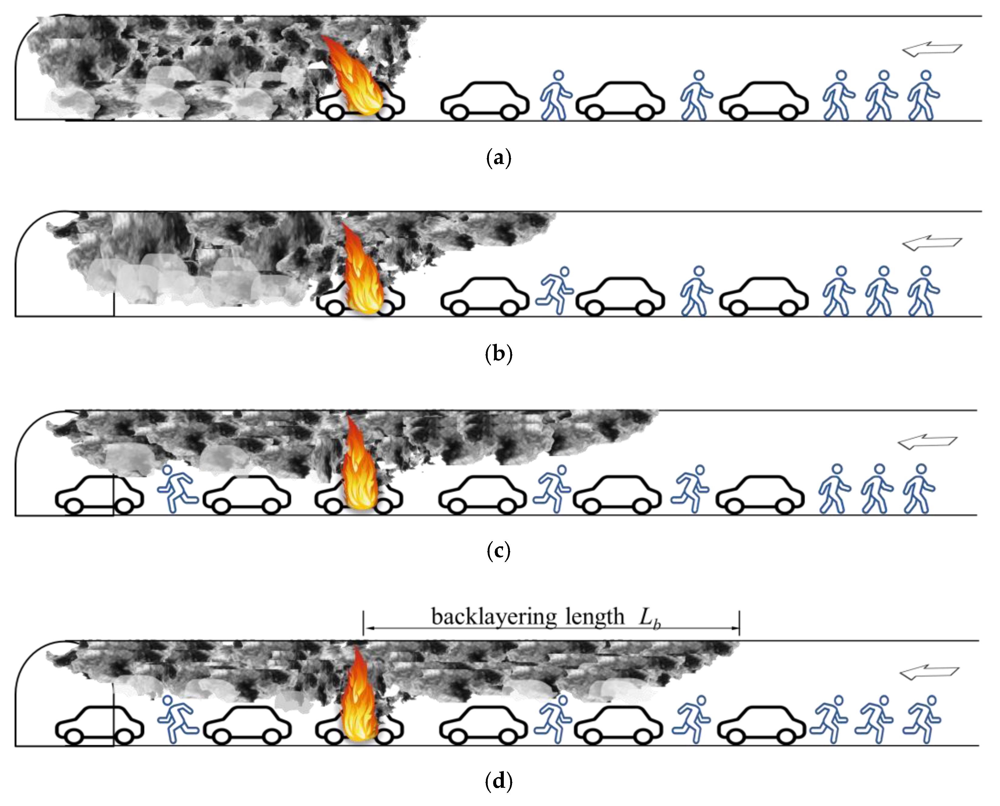
| Lb | Backlayering length of the thermal fume (m) |
| Lb* | Dimensionless backlayering length Lb*= Lb/H |
| M0 | No vehicular blockage |
| M1L | One side with low vehicular blockage |
| M1H | One side with high vehicular blockage |
| M2L | Both sides with low vehicular blockage |
| M2H | Both sides with high vehicular blockage |
| Qm | Average heat release rate (kW) |
| Q* | Dimensionless average heat release rate Q* = Qm) |
| R | Vehicular blockage ratio (Av/At) |
| Re | Reynolds number, Re = Um H/ν |
| Ri | Richardson number |
| t | Elapsed time after ignition (s) |
| T0 | Initial temperature (K)Ucr Critical velocity (m/s) |
| Um | Average ventilation longitudinal velocity in the cross-section (m/s) |
| W | The width of the tunnel (m) |
| Wo | The width of the obstacle (m) |
| x | Longitudinal axis of the tunnel |
| y | Transverse axis of the tunnel |
| z | Vertical axis (z = 0 is the floor) |
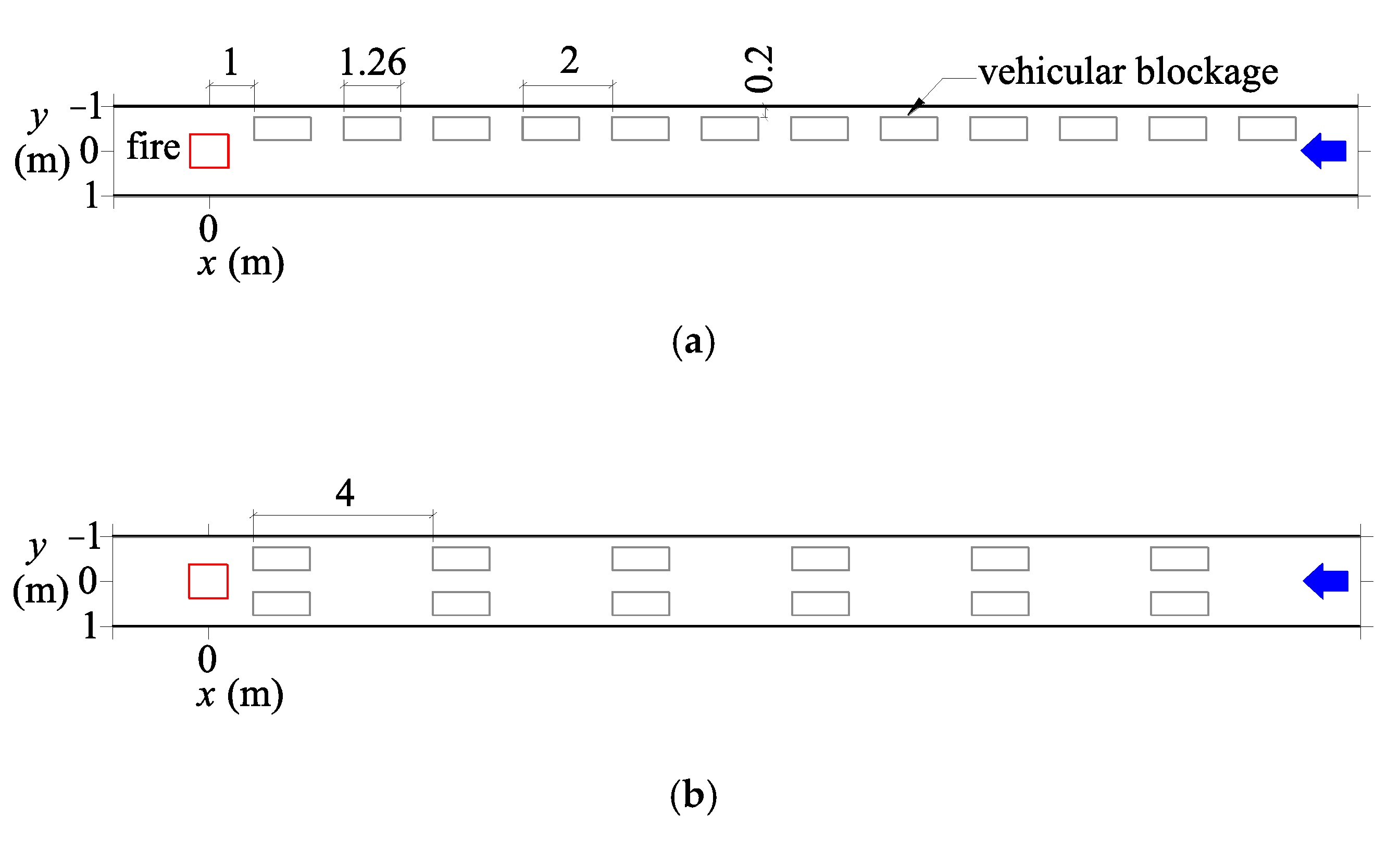
| Pattern A | The fire source is located in the center of the tunnel |
| Pattern B | The fire source is on the side of the tunnel |
| Greek letters | |
| α | Thermal diffusivity, α = λ/ρC (m2/s) |
| λ | friction coefficient |
| ν | Kinematic viscosity (m2/s) |
| ρ0 | Air density at ambient temperature (kg/m3) |
References
- PIARC Fire and Smoke Control. In PARIC Committee on Road Tunnels; World Road Association, Committee on Intelligent Transport (C16): La Défense, France, 1999; ISBN 2-84060-064-1.
- Fujita, K.; Minehiro, T.; Kawabata, N.; Tanaka, F. Temperature Characteristics of Backlayering Thermal Fume in a Tunnel Fire. J. Fluid Sci. Technol. 2012, 7, 275–289. [Google Scholar] [CrossRef] [Green Version]
- Mizuno, A.; Ohashi, H.; Nakahori, I.; Okubo, N. Emergency operation of ventilation for the Kanetsu road tunnel. In Proceedings of the 5th International Symposium on the Aerodynamics and Ventilation of Vehicle Tunnels, Lille, France, 20 May 1985; pp. 77–91. [Google Scholar]
- Mizuno, A. An optimal control with disturbance estimation for the emergency ventilation of a longitudinally ventilated road tunnel. In Flucome 91, Proceedings of the 3rd Triennial International Symposium on Fluid Control, Measurement, and Visualization, San Francisco, CA, USA, 1 June 1991; American Society of Mechanical Engineers: New York, NY, USA; pp. 393–399.
- Mizuno, A.; Ichikawa, A. Controllability of longitudinal air flow in transversely ventilated tunnels with multiple ventilation divisions. In Proceedings of the First International Conference on Safety in Road and Rail Tunnels, Basel, Switzerland, 23 November 1992; pp. 425–437. [Google Scholar]
- Vantelon, J.P.; Guelzim, A.; Quach, D.; Son, D.K. Investigation of Fire-Induced Smoke Movement in Tunnels and Stations: An Application to the Paris Metro. In Proceedings of the Third International Symposium on Fire Safety Science, Edinburgh, Scotland, 8 July 1991; pp. 907–918. [Google Scholar] [CrossRef] [Green Version]
- Saito, N.; Sekizawa, A.; Yamada, T.; Yanai, E.; Watanabe, Y.; Miyazaki, S. Study Report on Fire Performance in Special Space of Use of Underground Space. Fire Def. Res. Datum 1994, 29. [Google Scholar]
- Vauquelin, O.; Telle, D. Definition and Experimental Evaluation of the Smoke “Confinement Velocity” in Tunnel Fres. Fire Saf. J. 2005, 40, 320–330. [Google Scholar] [CrossRef]
- Hu, L.; Peng, W.; Huo, R. Critical wind velocity for arresting upwind gas and smoke dispersion induced by near-wall fire in a road tunnel. J. Hazard. Mater. 2008, 150, 68–75. [Google Scholar] [CrossRef] [PubMed]
- Minehiro, T.; Fujita, K.; Kawabata, N.; Hasegawa, M.; Tanaka, F. Backlayering Distance of Thermal Fumes in Tunnel Fire Experiments Using a Large-Scale Model. J. Fluid Sci. Technol. 2012, 7, 389–404. [Google Scholar] [CrossRef] [Green Version]
- Tang, F.; Li, L.; Mei, F.; Dong, M. Thermal smoke back-layering flow length with ceiling extraction at upstream side of fire source in a longitudinal ventilated tunnel. Appl. Therm. Eng. 2016, 106, 125–130. [Google Scholar] [CrossRef]
- Tanaka, F.; Takezawa, K.; Hashimoto, Y.; Moinuddin, K.A. Critical velocity and backlayering distance in tunnel fires with longitudinal ventilation taking thermal properties of wall materials into consideration. Tunn. Undergr. Space Technol. 2018, 75, 36–42. [Google Scholar] [CrossRef]
- Zhang, T.; Wang, G.; Li, J.; Huang, Y.; Zhu, K.; Wu, K. Experimental Study of Back-layering Length and Critical Velocity in Longitudinally Ventilated Tunnel Fire with Various Rectangular Cross-sections. Fire Saf. J. 2021, 126, 103483. [Google Scholar] [CrossRef]
- Kawabata, N.; Wang, Q.; Yagi, H.; Kawakita, M. Study of Ventilating Operation During Fire Accident in Road Tunnels with Large Cross Section. In Proceedings of the Fourth KSME-JSME Fluid Engineering Conference, Pusan, Korea, October 1998; pp. 53–56. [Google Scholar]
- Kunikane, Y.; Kawabata, N.; Yamada, T.; Shimoda, A. Influence of Stationary Vehicles on Backlayering Characteristics of Fire Plume in a Large Cross Section Tunnel. JSME Int. J. Ser. B 2006, 49, 594–600. [Google Scholar] [CrossRef] [Green Version]
- Li, Y.Z.; Lei, B.; Ingason, H. Study of critical velocity and backlayering length in longitudinally ventilated tunnel fires. Fire Saf. J. 2010, 45, 361–370. [Google Scholar] [CrossRef]
- Tang, W.; Hu, L.; Chen, L. Effect of blockage-fire distance on buoyancy driven back-layering length and critical velocity in a tunnel: An experimental investigation and global correlations. Appl. Therm. Eng. 2013, 60, 7–14. [Google Scholar] [CrossRef]
- Gannouni, S.; Ben Maad, R. Numerical study of the effect of blockage on critical velocity and backlayering length in longitudinally ventilated tunnel fires. Tunn. Undergr. Space Technol. 2015, 48, 147–155. [Google Scholar] [CrossRef]
- Zhang, S.; Cheng, X.; Yao, Y.; Zhu, K.; Li, K.; Lu, S.; Zhang, R.; Zhang, H. An experimental investigation on blockage effect of metro train on the smoke back-layering in subway tunnel fires. Appl. Therm. Eng. 2016, 99, 214–223. [Google Scholar] [CrossRef]
- Meng, N.; Liu, X.; Li, X.; Liu, B. Effect of blockage ratio on backlayering length of thermal smoke flow in a longitudinally ventilated tunnel. Appl. Therm. Eng. 2018, 132, 1–7. [Google Scholar] [CrossRef]
- Meng, N.; Yang, W.; Xin, L.; Li, X.; Liu, B.; Jin, X. Experimental study on backlayering length of thermal smoke flow in a longitudinally ventilated tunnel with blockage at upstream of fire source. Tunn. Undergr. Space Technol. 2018, 82, 315–324. [Google Scholar] [CrossRef]
- Lee, Y.-P.; Tsai, K.-C. Effect of vehicular blockage on critical ventilation velocity and tunnel fire behavior in longitudinally ventilated tunnels. Fire Saf. J. 2012, 53, 35–42. [Google Scholar] [CrossRef]
- Ejiri, Y.; Kawabata, N.; Mori, F. Large eddy simulation of fire in transverse ventilation tunnels. In Proceedings of the Tunnel Fires-Fifth International Conference, Melbourne, Australia, 3–7 October 2004; pp. 121–130. [Google Scholar]
- Tsai, K.-C.; Chen, H.-H.; Lee, S.-K. Critical ventilation velocity for multi-source tunnel fires. J. Wind Eng. Ind. Aerodyn. 2010, 98, 650–660. [Google Scholar] [CrossRef]
- Kunikane, Y.; Kawabata, N.; Takekuni, K.; Shimoda, A. Heat Release Rate Induced by Gasoline Pool Fire in a Large-Cross-Section Tunnel. Tunn. Manag. Int. 2003, 6, 22–29. [Google Scholar]
- Kawabata, N.; Kunikane, Y.; Yamamoto, N.; Takekuni, K.; Shimoda, A. Numerical Simulation of Smoke Descent in a Tunnel Fire Accident. Tunn. Manag. Int. 2003, 6, 357–366. [Google Scholar]
- Jang, H.-M.; Chen, F. On the determination of the aerodynamic coefficients of highway tunnels. J. Wind Eng. Ind. Aerodyn. 2002, 90, 869–896. [Google Scholar] [CrossRef]
- Oka, Y.; Atkinson, G.T. Control of smoke flow in tunnel fires. Fire Saf. J. 1995, 25, 305–322. [Google Scholar] [CrossRef]
- Kang, K. Characteristic length scale of critical ventilation velocity in tunnel smoke control. Tunn. Undergr. Space Technol. 2010, 25, 205–211. [Google Scholar] [CrossRef]


| Years | Research Topics | Authors | Research Methods | Obstacle Condition |
|---|---|---|---|---|
| 1991 | Investigation of Fire-Induced Smoke Movement in Tunnels and Stations: An Application to the Paris Metro [6]. | Vantelon, J.P.; Guelzim, A.; Quach, D.; Son, D.K. | Experimental method | No obstacles |
| 1994 | Study Report on Fire Performance in Special Space of Use of Underground Space [7]. | Saito, N.; Sekizawa, A.; Yamada, T.; Yanai, E.; Watanabe, Y.; Miyazaki, S. | Experimental method | No obstacles |
| 2005 | Definition and Experimental Evaluation of the Smoke “Confinement Velocity” in Tunnel Fres [8]. | Vauquelin, O.; Telle, D. | Experimental and simulation methods | No obstacles |
| 2008 | Critical Wind Velocity for Arresting Upwind Gas and Smoke Dispersion Induced by Near-Wall Fire in a Road Tunnel [9]. | Hu, L. H.; Peng, W.; Huo, R. | Experimental and simulation methods | No obstacles |
| 2012 | Backlayering Distance of Thermal Fume in Tunnel Fire Experiments Using a Large-Scale Model [10]. | Minehiro, T.; Fujita K.; Kawabata, N.; Hasegawa, M.; Tanaka, F. | Experimental and simulation methods | No obstacles |
| 2016 | Thermal Smoke Back-layering Flow Length with Ceiling Extraction at Upstream Side of Fire Source in a Longitudinal Ventilated Tunnel [11]. | Tang, F.; Li, L.J.; Mei, F.Z.; Dong, M.S. | Experimental and simulation methods | No obstacles |
| 2018 | Critical Velocity and Backlayering Distance in Tunnel Fires with Longitudinal Ventilation Taking Thermal Properties of Wall Materials into Consideration [12]. | Tanaka F.; Takezawa K.; Hashimoto Y.; Moinuddin K.A.M. | Experimental method | No obstacles |
| 2021 | Experimental Study of Back-layering Length and Critical Velocity in Longitudinally Ventilated Tunnel Fire with Various Rectangular Cross-sections [13]. | Zhang T.; Wang G.; Li J.; Huang Y.; Zhu K.; Wu K | Experimental method | No obstacles |
| 1998 | Study of Ventilating Operation During Fire Accident in Road Tunnels With Large Cross Section [14]. | Kawabata, N.; Wang, Q.; Yagi, H.; Kawakita, M. | Simulation method | More than two obstacles |
| 2006 | Influence of Vehicular blockage on Backlayering Characteristics of Fire Plume in a Large Cross Section Tunnel [15]. | Kunikane, Y.; Kawabata, N.; Yamada, T.; Shimoda, A. | Simulation method | More than two obstacles |
| 2010 | Study of Critical Velocity and Backlayering Length in Longitudinally Ventilated Tunnel Fires [16]. | Li, Y.Z.; Lei, B.; Ingason, H. | Experimental method | An obstacle |
| 2013 | Effect of Blockage-Fire Distance on Buoyancy Driven Backlayering Length and Critical Velocity in a Tunnel: An Experimental Investigation and Global Correlations [17]. | Tang, W.; Hu, L.H.; Chen, L.F. | Experimental method | An obstacle |
| 2015 | Numerical Study of the Effect of Blockage on Critical Velocity and Backlayering Length in Longitudinally Ventilated Tunnel Fires [18]. | Gannouni, S.; Maad, R.B. | Simulation method | An obstacle |
| 2016 | An Experimental Investigation on Blockage Effect of Metro Train on the Smoke Back-layering in Subway Tunnel Fires [19]. | Zhang, S.; Cheng, X.; Yao, Y.; Zhu, K.; Li, K.; Lu, S.; Zhang, R.; Zhang, H. | Experimental method | An obstacle |
| 2018 | Effect of blockage ratio on backlayering length of thermal smoke flow in a longitudinally ventilated tunnel [20]. | Meng, N.; Liu, X.; Li, X.; Liu, B. | Experimental method | An obstacle |
| 2018 | Experimental Study on Backlayering Length of Thermal Smoke Flow in a Longitudinally Ventilated Tunnel with Blockage at Upstream of Fire Source [21]. | Meng, N.; Yang, W.; Xin, L.; Li, X.; Liu, B.; Jin, X. | Experimental method | An obstacle |
| Type | Experimental Model | Actual Tunnel |
|---|---|---|
| Section shape | rectangular | rectangular |
| The width of the tunnel W (m) | 1.93 | 10 |
| The height of the tunnel H (m) | 1 | 5 |
| Tunnel cross-section area At (m2) | 1.93 | 50 |
| Froude number Fr | 0.07–0.39 | 0.07–0.39 |
| Dimensionless average heat re-lease rate Q* | 0.072 | 0.072 |
| Material (near the fire source) | ALC | concrete |
| Biot number Bi | 42.7–52.8 | 44.7–61.8 |
| Fourier numbers Fo | 6.41 × 10⁻⁸ | 1.72 × 10⁻⁸ |
| Csgs | Um (m/s) | Friction Factor λ | Average Velocity (m/s) | Turbulence Intensity (m/s) |
|---|---|---|---|---|
| 0.10 | 2.0 | Unstable | ||
| 0.12 | 2.0 | 0.0169 | 2.48 | 0.0845 |
| 0.14 | 2.0 | 0.0178 | 2.45 | 0.0874 |
| 0.15 | 2.0 | 0.0179 | 2.47 | 0.1033 |
| 0.17 | 2.0 | 0.0129 | 2.93 | 0.0208 |
| 0.20 | 2.0 | 0.0129 | 2.93 | 0.0001 |
| Tunnel | Vehicular Blockage | ||||||||||||
|---|---|---|---|---|---|---|---|---|---|---|---|---|---|
| x | y | z | x | y | z | ||||||||
| Length | Width | Height | Length | Width | Low Height | High Height | |||||||
| Grid number | Dim. (m) | Grid number | Dim. (m) | Grid number | Dim. (m) | Grid number | Dim. (m) | Grid number | Dim. (m) | Grid number | Dim. (m) | Grid number | Dim. (m) |
| 885 | 44.25 | 49 | 1.93 | 31 | 1 | 25 | 1.25 | 13 | 0.51 | 15 | 0.48 | 22 | 0.71 |
Publisher’s Note: MDPI stays neutral with regard to jurisdictional claims in published maps and institutional affiliations. |
© 2022 by the authors. Licensee MDPI, Basel, Switzerland. This article is an open access article distributed under the terms and conditions of the Creative Commons Attribution (CC BY) license (https://creativecommons.org/licenses/by/4.0/).
Share and Cite
Ho, Y.-T.; Kawabata, N.; Seike, M.; Hasegawa, M.; Chien, S.-W.; Shen, T.-S. Scale Model Experiments and Simulations to Investigate the Effect of Vehicular Blockage on Backlayering Length in Tunnel Fire. Buildings 2022, 12, 1006. https://doi.org/10.3390/buildings12071006
Ho Y-T, Kawabata N, Seike M, Hasegawa M, Chien S-W, Shen T-S. Scale Model Experiments and Simulations to Investigate the Effect of Vehicular Blockage on Backlayering Length in Tunnel Fire. Buildings. 2022; 12(7):1006. https://doi.org/10.3390/buildings12071006
Chicago/Turabian StyleHo, Yu-Tsung, Nobuyoshi Kawabata, Miho Seike, Masato Hasegawa, Shen-Wen Chien, and Tzu-Sheng Shen. 2022. "Scale Model Experiments and Simulations to Investigate the Effect of Vehicular Blockage on Backlayering Length in Tunnel Fire" Buildings 12, no. 7: 1006. https://doi.org/10.3390/buildings12071006