Article

A Novel Support-Vector-Machine-Based Grasshopper Optimization Algorithm for Structural Reliability Analysis

1
Science and Engineering Teaching and Research Office, Zhaoqing Open University, Zhaoqing 526000, China
2
Key Laboratory of Disaster Prevention and Structural Safety of Ministry of Education, College of Civil Engineering and Architecture, Guangxi University, Nanning 530004, China
3
Guangxi Provincial Engineering Research Center of Water Security and Intelligent Control for Karst Region, Guangxi University, Nanning 530004, China
*
Author to whom correspondence should be addressed.
Buildings 2022, 12(6), 855; https://doi.org/10.3390/buildings12060855
Submission received: 28 May 2022 / Revised: 15 June 2022 / Accepted: 15 June 2022 / Published: 19 June 2022
(This article belongs to the Section Building Structures)

Abstract

:
Aiming at the characteristics of high computational cost, implicit expression and high nonlinearity of performance functions corresponding to large and complex structures, this paper proposes a support-vector-machine- (SVM) based grasshopper optimization algorithm (GOA) for structural reliability analysis. With this method, the reliability problem is transformed into an optimization problem. On the basis of using the finite element method (FEM) to generate a small number of samples, the SVM model is used to construct a surrogate model of the performance function, and an explicit expression of the implicit nonlinear performance function under the condition of small samples is realized. Then, the GOA is used to search for the most probable point (MPP), and a reasonable iterative method is constructed. The MPP information of each iteration step is used to dynamically improve the reconstruction accuracy of the surrogate model in the region that contributes most to the failure probability. Finally, with the MPP after the iteration as the sampling center, the importance sampling method (ISM) is used to further infer the structural failure probability. The feasibility of the method is verified by four numerical cases. Then, the method is applied to a long-span bridge. The results show that the method has significant advantages in computational accuracy and computational efficiency and is suitable for solving structural reliability problems of complex engineering.

1. Introduction

The reliability of the structure helps to evaluate the performance of a part or the whole system, which is directly related to people’s safety. Structural reliability analysis is carried out around uncertainty, determined by random variables that represent and differentiate system performance, and based on the performance function of random variables [1]. The performance functions of large and complex engineering structures are often highly nonlinear and implicit. Their function values generally need to be obtained by means of numerical calculation methods, such as the finite element method (FEM), which usually consumes considerable time [2]. For traditional reliability problems, the mean-value first-order second moment (MVFOSM) method, the first-order second moment (FOSM) method and the second order reliability method (SORM) can achieve good results and have been widely used [3]. However, for complex problems with high computational cost, these methods are not suitable, because they require explicit expression of performance functions [4,5,6]. The Monte Carlo simulation (MCS) method and the importance sampling method (ISM) can obtain the ratio of the failure number to the total number of samples through a large number of random samplings to calculate the failure probability of structures. They are suitable for solving the structural reliability of implicit functions with high calculation accuracy. However, to ensure calculation accuracy, the random sampling times of the MCS method and ISM method are very large. In a recent study, Aroob et al. [7] conducted reliability analysis of fiber-reinforced polymer (FRP) reinforced panels by MCS method, and determined the specific target reliability index of the material, verifying the applicability of the MCS method in reliability analysis. For complex engineering structures, whose mechanical response to physical quantities, such as stress and deformation under load, are difficult to obtain directly through simple calculation formulas, the calculation time of single structural reliability analysis is very long, which leads to a great limitation of the MCS method and ISM method in practical engineering applications [8,9,10].
In recent years, the surrogate model method, which constructs explicit performance functions to approximate implicit performance functions in order to simplify calculation, has gradually emerged and become an important means to reduce the high computational cost in the process of reliability solution [11,12]. As a classical surrogate model, the response surface method (RSM) based on polynomial regression is widely used in the research of structural reliability analysis [13,14]. However, the reconstruction accuracy of this method is low in highly nonlinear problems. With the continuous development of machine learning in the field of artificial intelligence, machine learning models, such as artificial neural networks (ANN) [15], radial basis functions (RBF) [16], kriging [17], and support vector machines (SVM) [18,19] have been used as surrogate models of the actual performance function and achieved good results. Existing MCS-based surrogate model methods, such as ANN-MCS [20], RBF-MCS [21], and Kriging-MCS [22], have the advantages of clear concept, no need to calculate checkpoints, and easy implementation. However, models such as ANN and RBF have limitations, such as insufficient extrapolation ability and “overfitting” under the condition of small training samples, and these methods all have the problem of over-reliance on preset samples. Therefore, for reliability problems with high-dimensional random variables, a large number of preset samples are required to ensure the accuracy of the surrogate model. The number of samples grows exponentially with the increase in dimensions, resulting in high construction costs of surrogate models.
In order to reduce the construction cost of the surrogate model, some scholars in recent years have proposed to combine the bionic optimization algorithm with the surrogate model method to approximate the real failure domain boundary of the structure by using its powerful global optimization capability. Bionic optimization algorithm refers to the computing technology and method used to solve various optimization problems, developed by simulating the structural characteristics, evolutionary law, behavior and thinking structures of human, nature and other biological populations [23]. At present, the application scope of bionic optimization algorithm includes various fields, such as industry, agriculture, science, and technology. In the field of structural reliability, J. Cheng first combined ANN and genetic algorithm (GA), using ANN to import the explicit expression of approximate limit state function, so that GA became more effective after obtaining a clear limit state function, thus saving a lot of time-consuming finite element calculations [24]. In 2010, J. E. Hurtado and D. A. Alvarez combined the SVM surrogate model with the particle swarm optimization algorithm (PSO), and proposed a reliability evaluation idea different from MCS as the core [25]. In addition, the authors also pointed out that the swarm intelligence optimization algorithm can be combined with other machine learning models, which lays the foundation for the development of this method. Shortly afterwards, novel bionic optimization algorithms, such as the artificial bee colony algorithm (ABC) [26], the salp optimization algorithm (SOA) [27], and the firefly algorithm [28] were respectively combined with different surrogate models to further improve the computational efficiency of implicit and nonlinear reliability problems.
The purpose of this research is to establish a new dynamic updating surrogate model method to solve the problem of structural reliability with implicit, high nonlinear performance functions that are difficult to solve. In this method, a novel support-vector-machine-based grasshopper optimization algorithm (GOA) for structural reliability analysis is proposed. Combined with finite element calculation software and ISM, this algorithm has made great breakthroughs in solving problems that the implicit high nonlinear performance function cannot readily solve. The method is applied to an actual bridge project, and the results show that it has significant advantages in accuracy and efficiency, which verifies the superiority and practicability of this method in reliability analysis of complex structures.

2. Related Work

2.1. GOA

In 2017, a swarm intelligence optimization algorithm called GOA emerged, showing excellent global optimization capability [29]. The algorithm regards a single individual as a search operator and simulates the large-range fast movement of imagoes and local slow movement of larvae into global and local optimization, respectively. In the optimization process, with additional iterations, the global optimization stage is gradually transformed into the local optimization stage [
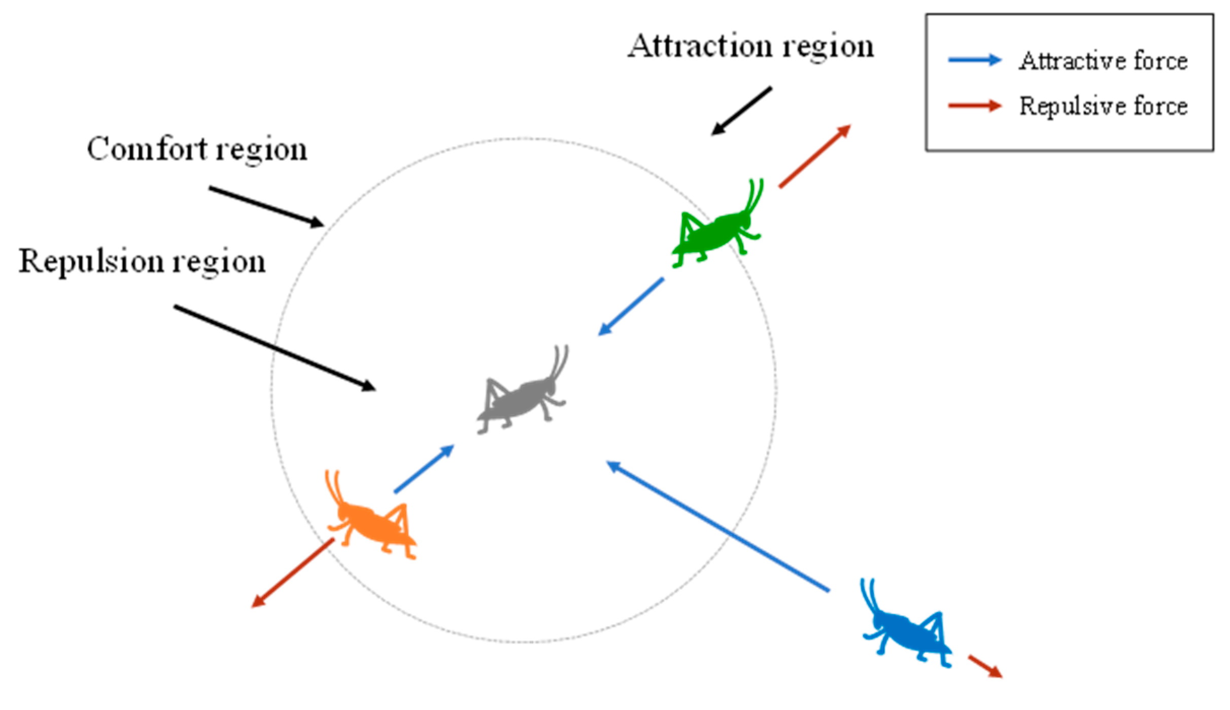
30]. In the stage of global optimization, the operator performs a rapid search in the model space over a large range to obtain the overall information of the model space and lock down a local area. In the stage of local optimization, the operator searches carefully in this local area and optimizes the accuracy of the solution through continuous iteration. According to the distance between the two operators, spatial regions can be divided into attractive regions, comfortable regions and repulsive regions (Figure 1).
When the distance between the two operators is relatively close (less than 2.079 units), they repulse each other, and the operator is in the repulsion region or within the repulsion distance. When the distance between the two operators is exactly 2.079 units, there is neither an attractive nor repulsive force, which is called the comfort region or the comfortable distance. In the same way, when the distance between two operators is more than 2.079 units, they attract each other, and thus this distance is called the attraction region or the distance of attraction [31]. According to this principle, grasshopper operators constantly adjust their positions with other operators to achieve optimization results.
It is important to note that there is no clear boundary between global and local optimization. With increasing iteration times, the search area gradually decreases, and the search gradually changes from global optimization to local optimization. The current grasshopper operator xi is defined by the grasshopper operator xj, as follows:
p d i j = m e d i j n e d i j x j x i d i j
where dij is the spatial distance between the current ith grasshopper operator and the jth grasshopper operator m and n are parameters to evaluate the effect of other agents on the agent; m represents the intensity of attraction, and n represents the spatial scale of attraction.
The next position of the grasshopper operator xi is defined as follows:
x i k ^ = c 1 j = 1 N c 2 u l k f l k 2 p d i j k x j k x i k d i j k + T g k
where x i k ^ is the position to which the i-th grasshopper operator moves next in the k-th dimension; N represents the total number of grasshopper operators; ulk and flk represent the upper and lower limits of the agent in the k-th dimension, respectively; d i j k denotes the spatial distance between the i-th grasshopper and the j-th grasshopper in the k-th dimension; x i k and x j k represent the current position of the i-th and j-th grasshoppers in the k-th dimension, respectively; T g k represents the component of the best solution found thus far in the k-th dimension, and c1 and c2 are known as adaptive shrinkage parameters, which maintain the relative balance between global and local optimization. If c1 and c2 are represented by c, their linear change can be calculated as:
c = c max t c max c min t max
where t represents the current iteration number; tmax represents the maximum number of iterations; cmax is the maximum value of the adaptive shrinkage parameter, and cmin is the minimum value of the adaptive shrinkage parameter.
The algorithm mainly contains six hyperparameters: the population number N, the maximum number of iterations tmax, and the upper and lower limits of the search ul and fl, respectively. The upper and lower limits of the search represent the search space of the model, which can be reasonably estimated according to actual problems. The number of populations and iterations have similar effects on the operation of the algorithm: when the number of populations or iterations increases, the search operator searches in more detail in the whole model space. If the population or iteration is too large, it causes many unnecessary searches, greatly increasing the running time of the algorithm and reducing the efficiency. However, if the population or iteration number is too small, the global optimal solution cannot be searched, which affects the accuracy of understanding. Therefore, it is necessary to constantly adjust these two parameters in a scientific way and select a group of population and iteration times that are more suitable for the current problem. The adaptive shrinkage parameter c gradually decreases with additional iterations so that the grasshopper algorithm does not converge quickly, thus affecting the proportion of the global optimization stage and local optimization stage. A large value of c in the early stage of the algorithm encourages the grasshopper operator to conduct global optimization, while a small value of c in the late stage of optimization encourages the grasshopper operator to conduct local optimization as much as possible and move towards the target.
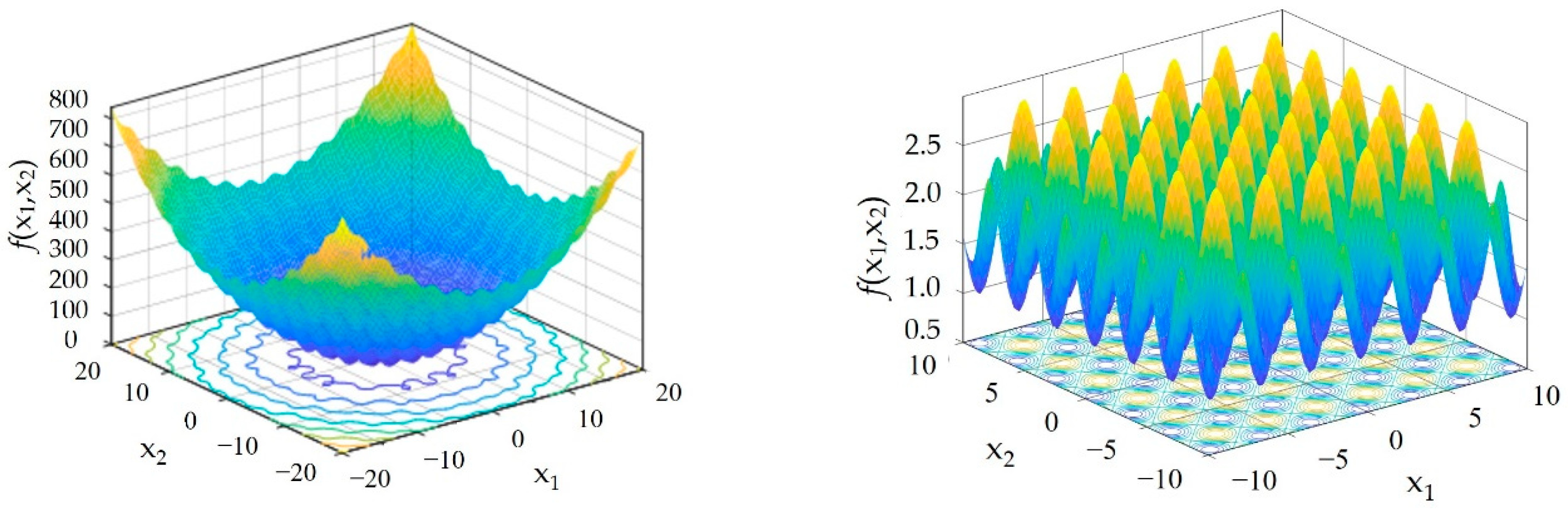
To demonstrate the good performance of the GOA, we adopt two common multi-modal test functions: the egg crate function and the periodic function (Figure 2), which are shown as Equations (4) and (5):
f ( x ) = f x 1 x n = i = 1 n ( x i 2 + 25 sin 2 ( x i ) ) x i [ 200 , 200 ] , i = 1 , 2 , , n
f ( x ) = f x 1 x n = 1 + i = 1 n sin 2 x i 0.1 e i = 1 n x i 2 x i [ 100 , 100 ] , i = 1 , 2 , , n
In the test process for the above two test functions, the dimension D of the test function is 5. In the egg crate function test, the parameter settings of the GOA are as follows: the population size N is 200, and the maximum number of iterations tmax is 500. In the periodic function test, the parameter settings of the GOA are as follows: the population size N is 100, and the maximum number of iterations tmax is 500. The calculation results are shown in Table 1. It can be seen that the difference between the optimal value searched by the algorithm and the minimum value of the function is very small. The difference between the average optimal value of the egg rate function and the minimum value of the function is only 3.99 × 10⁻¹¹, and the difference between the average optimal value of the periodic function and the minimum value of the function is only 4.65 × 10⁻⁵, indicating that the grasshopper algorithm has a strong global optimization ability.

2.2. SVM

The SVM [32] originated from pattern recognition in machine learning and is widely used, including portrait recognition, text classification, handwritten character recognition, bioinformatics and so on. In recent years, it has been applied to solve implicit nonlinear problems and has achieved good results. On the one hand, the SVM is very suitable for small sample fitting problems; on the other hand, the SVM can accurately represent high-dimensional functions and overcome the problem of dimension disaster. It can be divided into support vector classification (SVC) and support vector regression (SVR) according to the different functions used [33]. According to the properties of the hyperplane, the SVM can also be divided into linear and nonlinear.
In the SVM, the input is the sample of basic random variables, and the output is the response of the physical system. For a linearly separable problem yiy = {1, −1}, the analytic expression of the SVM is:
g x = w , x + b
where <.,.> represents the inner product in Rn, w∈Rn is the weight vector, and bR is the threshold.
Compared to SVC machines, the margin of SVR is replaced by a loss function. The original optimization model of the SVR problem can be expressed as:
min J = 1 2 w 2 + C i = 1 m ξ i + ξ i * s . t . y i w , x i b < ε + ξ i i 1 , , m ξ i + ξ i * R + × R +
where ξ i , ξ i * R + , n × R + , n is the relaxation variable and C is the penalty parameter.
By introducing the corresponding Lagrange function, the SVM formula for linear problems can be derived:
g x = i = 1 m α i α i * x , x i + b
where (ααi) is a Lagrange multiplier and must be positive.
However, real problems are often non-linear. To extend Equation (8) to nonlinear functions, we can replace the inner product directly with the kernel function:
g x = i = 1 m α i α i * K x , x i + b
where K x , x i is the kernel function.
There are many kinds of kernel functions of SVM, such as linear kernels, polynomial kernels, neural network kernels, and Markov kernels. One of its advantages is that the model performance can be improved by selecting appropriate kernel functions. Therefore, it is very important to choose an appropriate kernel function for a particular problem. The Gaussian RBF kernel is adopted in this paper, whose expression is given below:
k x 1 , x 2 = exp 1 2 σ 2 x 1 x 2 2
where σ is the width parameter.

3. The Proposed SVM-Based GOA Method

3.1. Basic Concept

In the standard normal space, the geometric meaning of the reliability index is the shortest distance from the origin of coordinates to the limit state equation. According to the geometric meaning of the reliability index, the structural reliability can be solved as the following equation for the constrained optimization problem:
Min β = i = 1 n X i μ i σ i 2 s . t .   g X = g x 1 , x 2 , , x n = 0
where X is a random variable, g(X) is a performance function, μi is the mean value of all design variables, and σi is the standard deviation of all design variables.
By using the penalty function method, the above equation for the constrained optimization problem can be transformed into the following unconstrained optimization problem:
Min β = i = 1 n X i μ i σ i 2 + P g X 2
where P is the penalty coefficient, which is generally a large constant.
The optimal algorithm is used to solve the above optimization problems, and the obtained solution is generally called the most probable point (MPP), which is the point with the largest contribution to the failure probability in the failure domain. For complex structures that are time-consuming for a single calculation, the basic principle for achieving rapid reliability analysis is as follows: On the premise of ensuring a certain calculation accuracy, we aim to reduce the number of finite element reanalysis calculations.
To achieve high efficiency and precision of reliability analysis, the steps involved in the proposed method are listed as follows:
  • Using the GOA to solve the reliability index
The GOA, with its excellent searching performance, is used to quickly search the global optimal solution (MPP) of Equations (11) or (12). When the grasshopper operator finds the information of the probable optimal solution in this region, it uses the information as a new knowledge source to replace the old operator and improves the prediction ability of the SVM model by updating knowledge and gradually approaching the optimal region to predict the particles closer to the optimal solution.
b.
Using the SVM model to construct the surrogate model
In view of the advantages of SVM’s strong generalization ability under the condition of small samples, a small number of samples are used to train the SVM model as a surrogate model for performance functions, thereby establishing a nonlinear mapping relationship between random variables and functional function values. This not only ensures that the sample generation process does not call too many time-consuming finite element programs, but also ensures that performance functions with strong nonlinearity can be reasonably approximated.
c.
Using a dynamic surrogate model strategy to improve the calculation accuracy
The key to the surrogate model method is whether it can fit the region near the point where the maximum contribution to the failure probability of the structure occurs within the failure region. Therefore, this paper constructs an iterative process to achieve dynamic updating of surrogate models. In each iteration process, the new MPP searched by GOA is substituted into the finite element model, and the real performance function value is calculated to obtain a new sample. Then, the new sample is added into the original sample set to retrain the SVM model. By iteratively repeating this process, the fitting error of the SVM surrogate model in the region near the limit state equation can be adaptively corrected. It should be pointed out that only one FEA is required for each iterative step. However, the fitting accuracy is effectively improved, thereby reducing the dependence of the fitting effect on the preset samples and accelerating the convergence speed of the iterative calculation.
d.
Using ISM to further improve computational accuracy
Through the iterative calculation of the GOA-SVM collaborative algorithm, the MPP and its corresponding reliability index can be obtained. However, when the performance function in the vicinity of the MPP is strongly nonlinear, the failure probability directly derived from the reliability index may still have a large error, as shown in Figure 3. Therefore, with MPP as the sampling center, the importance sampling method is used to calculate the failure probability, which can further improve the calculation accuracy.
The basic idea of the ISM is to change the center of random sampling so that the sample points have more chances to fall into the failure domain and increase the chance of structure performance function Z ≤ 0. Let the structural performance function be Z = g(X) and the joint probability density function of the random variable X be fx(x); then, the structural failure probability is
P f = + I g X x f X x d x
where I(x) is an indicative function of x. I(x) = 1 when x < 0, and 0 otherwise.
Assuming that the importance sampling probability density function is PV(v), Equation (13) can be rewritten as
P f = + I g X v f X v P V v P V v d v
If PV(v) is used to sample V, vk(vk1, vk2, …, vkn)T (k = 1, 2, …, N) is obtained. When each variable xi is independent of each other, the unbiased estimate of pf is
p f = 1 N k = 1 N I g v k i = 1 n f X i v k i p V i v k i

3.2. Procedures

The method is realized as shown in Figure 4, and the specific steps are as follows:
Step 1:
According to the characteristic distribution of random variable x, the real performance function values g x 1 , x 2 , , x n and g x 1 , x 2 , , x i ± f σ i , , x n are calculated by the experimental design method. Then, m = 2n + 1 initial training samples are constructed, where the interpolation coefficient f is generally 2.
Step 2:
Train the SVM surrogate model. The nonlinear mapping relationship between random variables and performance function values is established.
Step 3:
According to Equation (12), the global optimal solution, namely, the MPP, is searched through the GOA to obtain the corresponding reliability index.
Step 4:
According to the convergence evaluation formula: β w β w 1 < 10 3 (absolute difference of reliability index in successive iteration steps), if convergence is not satisfied, the MPP and its real function value are re-input into the original training sample set, and we return to Step 2. Otherwise, convergence is satisfied, and the iteration ends.
Step 5:
The MPP obtained in the final iteration step is taken as the sampling center of gravity. According to Equation (15) above, the ISM method is adopted to calculate the failure probability.

4. Results and Discussion

To verify the feasibility of this method, four numerical examples are given. Cases 1 and 2 are reliability problems with explicit performance functions that can be assumed to be “implicit” to investigate the feasibility of the method, while Cases 3 and 4 are examples of structures with implicit performance functions. In addition, after preliminary tests, the polynomial kernel function, RBF kernel function, and sigmoid kernel function of SVM were used in the following four cases, and the results had little difference. However, the calculation time using the polynomial kernel function was the shortest, so the polynomial kernel function and its corresponding parameters were used in the following cases.

4.1. Case 1

A nonlinear performance function is given as:
g x = exp 0.4 x 1 + 2 + 7.0 exp 0.3 x 2 + 5.0 200
where x1 and x2 are normally distributed.
The parameters of the GOA algorithm are set to N = 20, Cmax = 1.0, Cmin = 1.0 × 10⁻⁵, and P = 1000. The polynomial kernel function of SVM is selected, and the parameters of SVM model are set to C = 45 (C is the penalty coefficient), and d = 3 (d is the order). Five initial training samples are generated using the Bucher experimental design, as shown in Table 2. As seen from Table 2, the SVM-predicted value is very close to the true function value. The relative errors of the other three randomly selected test samples are shown in Table 3. It can be seen from this that the maximum relative error is less than 5%, indicating that the trained SVM model can well approximate the original performance function, thus replacing the original performance function for MCS sampling. The calculation results are shown in Table 4. When the results of 106 MCS simulations are used as the exact solution, compared with methods such as RSM and RBF-based FORM, the results of the proposed method are very close to the reference exact solution, and the number of finite element operations is low: only 1/30 of the RBF-based FORM.

4.2. Case 2

A nonlinear performance function is given as:
g x = x 1 2 + 4 x 2 1 20 + sin 5 2 x 1 + 2
where x1~N(1.5,1) and x2~N(2.5,1).
The parameters of the GOA algorithm are set to N = 20, Cmax = 1.0, Cmin = 1.0 × 10⁻⁵, and P = 1000. The polynomial kernel function of SVM is selected, and the parameters of SVM model are set to C = 45, and d = 3. Five initial training samples are predefined by the Bucher experimental design, as shown in Table 5.
The calculation results are shown in Table 6. The result of the FORM method is very poor, and there is a large gap in accuracy and efficiency. Although the RSM method has fewer function calls, the relative error is as high as 94.29%, which means the method has poor fitting accuracy. The problem can be solved more precisely with the GOA method. However, the method in this paper is superior to the GOA method in terms of the number of function calls and relative errors. This case verifies the feasibility of the method in this paper for solving the reliability problem of highly nonlinear implicit performance functions, and effectively overcomes the limitation of the low computational accuracy of traditional methods, such as the FORM and RSM, in solving such problems. Furthermore, it also proves that GOA-SVM outperforms the GOA method by a large margin in terms of computational efficiency.

4.3. Case 3

A plane portal frame is shown in Figure 5. The elastic modulus of each unit is 2.0 × 10⁶ kN/m2, and the relationship between the moment of inertia of the section and the section area is Ii = αiAi2. Taking the horizontal displacement D(x) of node 3 as the maximum deformation control, the structure performance function is
g u 3 = 0.01 D x
where [u] is the maximum allowable displacement, which is taken as 0.01 m. The statistical characteristics of the cross-sectional area of random variables A1 and A2 and the concentrated load P are shown in Table 7.
The parameters of the GOA algorithm are set to N = 20, Cmax = 1.0, Cmin = 1.0 × 10⁻⁵, and P = 1000. The polynomial kernel function of SVM is selected, and the parameters of the SVM model are set to C = 45 and d = 3. Four methods are proposed to calculate the displacement response value, and the results are shown in Table 8. The result of the MCS method is used as the reference solution. Compared with methods such as RSM and ANN-MCS, the calculation accuracy of the proposed method is the closest to the exact solution, and the number of function calls is 34% of that of RSM and 42% of that of ANN-MCS.

4.4. Case 4

A ten-bar truss structure is shown in Figure 6, in which the cross-sectional area of each bar is Ai(i = 1, 2, …, 10), the elastic modulus is E, and the external loads are P1, P2, and P3. There are 15 basic random variables in total, and they all obey the normal distribution. The statistical parameters are shown in Table 9. The function is established with the specification of node 2, not allowing the vertical displacement D(x) to exceed 4 mm:
g X = 0.004 D X
This is a high-dimensional implicit performance function structural reliability problem. The vertical displacement D(x) in the functional function is calculated by ANSYS FEA software.
The parameters of the GOA algorithm are set to N = 20, Cmax = 1.0, Cmin = 1.0 × 10⁻⁵, and P = 1000. The polynomial kernel function of SVM is selected, and the parameters of SVM model are set to C = 45, and d = 3. The calculation results of different methods are shown in Table 10. It can be seen that the relative error of the RSM method is the largest. The results of the SVM-based FORM are not much different from the results of the method in this paper, but the number of finite element calls required by the method in this paper is reduced by 66%, indicating that it has good adaptability to the structural reliability problem of high-dimensional implicit functions.

5. Engineering Application

A two-way six-lane suspension bridge is 1440 m long and has a main span of 616 m in two directions. The south tower of the bridge is 118.972 m high, and the north tower is 139.704 m high. The general arrangement of the bridge is shown in Figure 7 [35].
According to the General Specification for Highway Bridge Design of China (JTG D60-2004), the maximum allowable vertical deflection of the main girder under vehicle loading (excluding impact) is [u] = L/400 = 616/400 = 1.54 m. The normal use state performance function is given as:
g x = 1.54 u v x
where uv(x) is the maximum vertical deflection of the main beam, which can be calculated by ANSYS finite element software.
In the process of static reliability analysis of the bridge, the finite element software ANSYS is needed to calculate the structural response of the MPP generated in the initial training sample and the iteration step, namely, the real performance function values. Figure 8 shows the ANSYS model. In the modeling process, the main tower and the main beam use spatial beam elements, and the main cable and hanger use spatial truss elements. Master–slave constraints are established between the main tower and girder and the double cable planes. The connection between the main tower and the foundation is simplified to a solid connection. In the lower beam of the main tower, the main girder and the beam are set up by rigid arms in the Z and Y directions, with the X-axis along the bridge direction, the Y-axis along the transverse bridge direction, and the Z-axis vertical. In the ANSYS command stream, the random variables of bridge reliability analysis are set as variables, and ANSYS is started directly through the MATLAB executable file in the analysis. The random variables obtained in the MATLAB program analysis are assigned to the corresponding variables in the ANSYS command stream through the data interface file, and the structural response value is obtained. Then, the structural response value obtained by ANSYS is returned to MATLAB to calculate the functional state of the structure through the data interface file, which ensures smooth progress of the iterative program in MATLAB.
The parameters of the GOA algorithm are set to N = 20, Cmax = 1.0, Cmin = 1.0 × 10⁻⁵, and P = 1000. The polynomial kernel function of SVM is selected, and the parameters of SVM model are set to C = 45, and d = 3. This computation is carried out on a PC (Intel Core i5-2320 CPU @ 3.0 GHz).
The calculation results are shown in Table 11. It can be seen that compared with the RSM method, the method in this paper is closer to the calculation results of the MCS method, and the number of function calls in the finite element software is approximately 1/4 that of the RSM. The engineering application shows that the proposed method has good applicability in the reliability analysis of complex structures.

6. Conclusions

This paper combines the GOA, the SVM model and the ISM method and proposes a new structural reliability analysis method called the GOA-SVM-based dynamic surrogate model. This method not only makes use of the characteristics of the GOA, which can quickly and accurately search for the MPP of highly nonlinear performance functions in the global space, but also makes full use of the strengths of the SVM model, which effectively reduces errors and improves accuracy through the establishment of the dynamic response correction mechanism and the introduction of the ISM. The results show that the proposed method can efficiently and accurately solve the reliability problem of multi-peak highly nonlinear performance functions. It effectively solves the problems of large calculation errors or non-convergence of iterations that occur when the structural performance function is highly nonlinear or the failure probability is low, and overcomes the shortcomings of over-reliance on preset samples. Moreover, it is easy to combine with the existing FEA software or structural analysis program, which is convenient for practical engineering applications.

Author Contributions

Conceptualization, Y.Y. and G.S.; methodology, W.S. and G.S.; software, W.S.; validation, Y.Y., W.S. and G.S.; investigation, W.S.; data curation, W.S.; writing—original draft preparation, W.S.; writing—review and editing, Y.Y., W.S. and G.S.; visualization, W.S.; project administration, Y.Y.; funding acquisition, G.S. All authors have read and agreed to the published version of the manuscript.

Funding

This research was funded by the National Natural Science Foundation of China for financial support (Grant Nos. 52169021 and 51869003), and the High Level Innovation Team and Outstanding Scholar Program of Universities in Guangxi province. (Grant No. 202006).

Institutional Review Board Statement

Not applicable.

Informed Consent Statement

Not applicable.

Data Availability Statement

Not applicable.

Conflicts of Interest

The authors declare no conflict of interest.

References

  1. Alkhatib, S.; Deifalla, A. Reliability-based assessment and optimization for the two-way shear design of lightweight reinforced concrete slabs using the ACI and EC2. Case Stud. Constr. Mat. 2022, 17, e01209. [Google Scholar] [CrossRef]
  2. Antonio, C. A hierarchical genetic algorithm for reliability based design of geometrically non-linear composite structures. Compos. Struct. 2001, 54, 37–47. [Google Scholar] [CrossRef]
  3. Alkhatib, S.; Deifalla, A. Punching Shear Strength of FRP-Reinforced Concrete Slabs without Shear Reinforcements: A Reliability Assessment. Polymers 2022, 14, 1743. [Google Scholar] [CrossRef] [PubMed]
  4. Low, B.K. FORM, SORM, and spatial modeling in geotechnical engineering. Struct. Saf. 2014, 49, 56–64. [Google Scholar] [CrossRef]
  5. Skrzypczak, I.; Słowik, M.; Buda-Ożóg, L. The application of reliability analysis in engineering practice—Reinforced concrete foundation. Procedia Eng. 2017, 193, 144–151. [Google Scholar] [CrossRef]
  6. Farag, R.; Haldar, A. A novel concept for reliability evaluation using multiple deterministic analyses. INAE Lett. 2016, 1, 85–97. [Google Scholar] [CrossRef] [Green Version]
  7. Ateyat, A.; Mostafa, O.; Alotaibi, E.; Barakat, S. Reliability-based calibration for punching shear reduction factor for FRP reinforced slabs. In Proceedings of the 2022 Advances in Science and Engineering Technology International Conferences (ASET), Dubai, United Arab Emirates, 21–24 February 2022; pp. 1–6. [Google Scholar]
  8. Palle, T.; Michael, B. Structural Reliability Theory and Its Applications; Springer Science & Business Media: Berlin, Germany, 1982. [Google Scholar]
  9. Hu, J.; Yan, L.; Liu, F.; Duan, Q.; Zhang, Z. Reliability-based structural integrity assessment of Liquefied Natural Gas tank with hydrogen blistering defects by MCS method. In Proceedings of the 6th International Conference on Natural Computation, Yantai, China, 10–12 August 2010. [Google Scholar]
  10. Su, G.; Yu, B.; Xiao, Y.; Yan, L. Gaussian Process machine-learning method for structural reliability analysis. Adv. Struct. Eng. 2014, 17, 1257–1270. [Google Scholar] [CrossRef]
  11. Kaymaz, I.; Mcmahon, C.A. A response surface method based on weighted regression for structural reliability analysis. Probab. Eng. Mech. 2005, 20, 11–17. [Google Scholar] [CrossRef]
  12. Gomes, H.M.; Awruch, A.M. Comparison of response surface and neural network with other methods for structural reliability analysis. Struct. Saf. 2004, 26, 49–67. [Google Scholar] [CrossRef]
  13. Kim, S.; Na, S. Response surface method using vector projected sampling points. Struct. Saf. 1997, 19, 3–19. [Google Scholar] [CrossRef]
  14. Wahab, M.; Kurian, V.J.; Liew, M.S.; Nizamani, Z.; Kim, D.K. Structural reliability analysis using quadratic polynomial response surface and finite element in MATLAB. In Proceedings of the Asme International Conference on Ocean, Busan, Korea, 19 June 2016. [Google Scholar]
  15. Jha, B.N.; Li, H. Structural reliability analysis using a hybrid HDMR-ANN method. J. Cent. South Univ. 2017, 24, 2532–2541. [Google Scholar] [CrossRef]
  16. Jing, Z.; Chen, J.; Li, X. RBF-GA: An adaptive radial basis function metamodeling with genetic algorithm for structural reliability analysis. Reliab. Eng. Syst. Saf. 2019, 189, 42–57. [Google Scholar] [CrossRef]
  17. Zhang, L.; Lu, Z.; Wang, P. Efficient structural reliability analysis method based on advanced Kriging model. Appl. Math. Model. 2015, 39, 781–793. [Google Scholar] [CrossRef]
  18. Rocco, C.M.; Moreno, J.A. Fast Monte Carlo reliability evaluation using support vector machine. Reliab. Eng. Syst. Saf. 2002, 76, 237–243. [Google Scholar] [CrossRef]
  19. Alibrandi, U.; Alani, A.; Koh, C.G. Implications of high-dimensional geometry for structural reliability analysis and a novel linear response surface method based on SVM. Int. J. Comput. Methods 2015, 12, 1540016. [Google Scholar] [CrossRef]
  20. Kaymaz, I. Application of kriging method to structural reliability problems. Struct. Saf. 2005, 27, 133–151. [Google Scholar] [CrossRef]
  21. Deng, J.; Gu, D.; Li, X.; Yue, Z.Q. Structural reliability analysis for implicit performance functions using artificial neural network. Struct. Saf. 2005, 27, 25–48. [Google Scholar] [CrossRef]
  22. Deng, J. Structural reliability analysis for implicit performance function using radial basis function network. Int. J. Solids Struct. 2006, 43, 3255–3291. [Google Scholar] [CrossRef] [Green Version]
  23. Kar, A. Bio inspired computing—A review of algorithms and scope of applications. Expert Syst. Appl. 2016, 59, 20–32. [Google Scholar] [CrossRef]
  24. Cheng, J. Hybrid genetic algorithms for structural reliability analysis. Comput. Struct. 2007, 85, 1524–1533. [Google Scholar] [CrossRef]
  25. Hurtado, J.; Alvarez, D. An optimization method for learning statistical classifiers in structural reliability. Probab. Eng. Mech. 2010, 25, 26–34. [Google Scholar] [CrossRef]
  26. Luo, X.; Li, X.; Zhou, J.; Cheng, T. A Kriging-based hybrid optimization algorithm for slope reliability analysis. Struct. Saf. 2012, 34, 401–406. [Google Scholar] [CrossRef]
  27. Zhong, C.; Wang, M.; Dang, C.; Ke, W. Structural reliability assessment by salp swarm algorithm-based FORM. Qual. Reliab. Eng. 2020, 36, 1224–1244. [Google Scholar] [CrossRef]
  28. Yan, Y. Performance Prediction by an SVM with a Firefly Optimization Method. Int. J. Reliab. Qual. Saf. Eng. 2020, 3, 17–29. [Google Scholar] [CrossRef]
  29. Li, J.; Sun, W.; Su, G.; Zhang, Y. An intelligent optimization back-analysis method for geomechanical parameters in underground engineering. Appl. Sci. 2022, 12, 5761. [Google Scholar] [CrossRef]
  30. Saremi, S.; Mirjalili, S.; Lewis, A. Grasshopper optimisation algorithm: Theory and application. Adv. Eng. Softw. 2017, 105, 30–47. [Google Scholar] [CrossRef] [Green Version]
  31. Saxena, A. A comprehensive study of chaos embedded bridging mechanisms and crossover operators for grasshopper optimisation algorithm. Expert Syst. Appl. 2019, 132, 166–188. [Google Scholar] [CrossRef]
  32. Vanpik, V. The Nature of Statistical Learning Theory; Springer: New York, NY, USA, 2013; pp. 200–218. [Google Scholar]
  33. Sui, W.; Zhang, D.; Qiu, X.; Zhang, W. Prediction of the remaining useful life of rolling bearings based on mutual information and SVR. In Proceedings of the IOP Conference Series Materials Science and Engineering, Iasi, Romania, 16–17 May 2019. [Google Scholar]
  34. Li, H.; Lv, Z.; Zhao, J. A support vector machine method for reliablility analysis based on weighted linear response surface. Eng. Mech. 2007, 7, 67–71. [Google Scholar]
  35. Su, G.; Peng, L.; Hu, L. A Gaussian process-based dynamic surrogate model for complex engineering structural reliability analysis. Struct. Saf. 2017, 68, 97–109. [Google Scholar] [CrossRef]
Figure 1. The figure of the interaction between individual grasshoppers.
Buildings 12 00855 g001
Figure 2. The figures of multi-modal test functions. (a) The egg crate function; (b) the periodic function.
Buildings 12 00855 g002
Figure 3. Regression result comparison among different models.
Buildings 12 00855 g003
Figure 4. Flowchart of the SVM-based GOA method.
Buildings 12 00855 g004
Figure 5. Planar frame structure.
Buildings 12 00855 g005
Figure 6. Ten-bar truss.
Buildings 12 00855 g006
Figure 7. General arrangement of the bridge [35].
Buildings 12 00855 g007
Figure 8. Model diagram in ANSYS.
Buildings 12 00855 g008
Table 1. Test results of the two benchmark functions.
Test FunctionThe Maximum Number of IterationsThe Minimum ValueThe Average Optimal Value
Egg crate50003.99 × 10−11
Periodic5000.90.9 + (4.65 × 10⁻⁵)
Table 2. The initial training samples and function values of Case 1.
Numberx1x2Truth Value of the Performance FunctionPredictive Value of the Performance FunctionRelative Error/%
1−0.190.43648.72648.720.00
21.34−0.691554.881554.880.00
3−0.05−0.96764.36764.360.00
4−1.28−0.60332.25332.250.00
5−0.34−0.73636.31636.310.00
Table 3. The test samples and function values of Case 1.
Numberx1x2Truth Value of the Performance FunctionPredictive Value of the Performance FunctionRelative Error/%
10.510.351018.18978.864.0
20.280.30926.06891.893.8
30.030.02784.24761.982.9
Table 4. Comparison of calculation results of Case 1.
MethodMCS [13]RSM(f = 2)RBF-FORMSVM-GOA
Pf/10−33.633.523.213.60
Relative error/%-3.0311.570.83
Function calls1063129610
Table 5. The initial training samples and function values of Case 2.
Numberx1x2Truth Value of the Performance FunctionPredictive Value of the Performance FunctionRelative Error/%
1−202.312.310.00
20−22.602.600.00
3202.492.490.00
4021.801.800.00
5002.202.200.00
Table 6. Comparison of calculation results of Case 2.
MethodMCSRSMFORMGOASVM-GOA
Pf/10−33.150.1830.223.323.18
Relative error/%-94.291059.375.400.95
Function calls106192501269
Table 7. The statistical parameters in Case 3.
Random VariablesDistributionUnitMeanCovαi
A1Lognormalm20.360.0360.0833
A2Lognormalm20.180.0180.1667
PExtreme value type I kN205.0-
Table 8. Comparison of calculation results of Case 3.
MethodMCSRSMANN-MCS [20]SVM-GOA
Pf/10−32.81602.84052.83382.8135
Relative error/%-0.8700.6320.089
Function calls106413316
Table 9. The statistical parameters in Case 4.
Random VariablesDistributionUnitMeanCov
LLognormalm10.05
AiLognormalm20.0010.00015
ELognormalGPa1005
P1LognormalkN804
P2LognormalkN100.5
P3LognormalkN100.5
Table 10. Comparison of calculation results of Case 4.
MethodMCS [34]RSM [34]SVM-FORM [34]SVM-GOA
Pf/10−34.6432.6264.7564.723
Relative error/%-43.442.431.72
Function calls10615515552
Table 11. Comparison of calculation results.
MethodMCSRSMSVM-GOA
Reliability index2.362.592.34
Relative error/%-9.750.85
Function calls10625552
Computing time/min506,000131.827.9
Publisher’s Note: MDPI stays neutral with regard to jurisdictional claims in published maps and institutional affiliations.

