Parameter Optimization and Application for the Inerter-Based Tuned Type Dynamic Vibration Absorbers

Abstract

As an acceleration-type mechanical element, inerter element has been widely used in the dynamic suppressing field. In this paper, a tuned mass damper with inerter (TMDI) is presented for vibration control and energy dissipation. To evaluate the effectiveness of the TMDI, the simplified model of TMDI coupled with a single-degree-of-freedom (SDOF) structure has been established. Numerical optimization has been conducted with the goal of minimizing the maximum transfer function amplitude of displacement for the damped primary structure. The control performance and robustness for TMDI has been evaluated with the SDOF system in the frequency and time domain, compared with the classical TMD device. Lately, multiple active TMDI (MATMDI) has been proposed as a vibration suppression strategy for a multi-story steel structure. The performances of passive and active control methods have been evaluated in the time domain via real earthquake excitations, and it has proven that the MATMDI is more effective at reducing the response of the structure and the stroke of devices. The results show that the proposed optimal TMDI system can sufficiently harvest vibrational energy and enhance the robustness of structure.

1. Introduction

Lately, with the development of enormous activities, an ever-increasing number of structures are being constructed in the seismically dynamic regions. One of the most efficient methods to reduce earthquake-induced structural vibrations is to employ external vibration-control system on the structures. For instance, the base isolation [1], additional buckling-restraint bracing [2], and auxiliary dampers [3] can be added to the structure. Among them, the tuned mass damper (TMD) is a device with easy manufacture and disassembly, that is widely utilized in the structural vibration mitigation field [4]. It can be found in the existing large-scale and ultra-high structures, such as Taipei 101 [5], Citicorp Center in New York City [6], the Sydney TV Tower in Australia [7], and the Shanghai Center Tower in China [8]. It works on a simple principle. By altering the frequency of TMD, so that it could oscillate with the same period as the host structure, it absorbs and dissipates energy [9,10] from the main structure.

The TMD system is composed of the mass block, spring, and damping element. The component of TMD is pretty convenient. However, it is a challenges for the parameter design concerning obtaining the most reliable control efficacy. The fixed-point theory was first proposed by Den Hartog [11] to obtain the optimal parameters of TMD when it is attached to the undamped single-degree-of-freedom (SDOF) system. Further, Warburton et al. [12] summarized the analytical expressions for the optimal design parameters under various excitation conditions. Asami et al. [13] used the $H_{\infty }$ and $H_2$ optimization approaches to acquire the analytical TMD solutions, considering the structural response under random excitation. While, for damped structures, it is hard to achieve the ideal design parameters by theoretical derivation, numerical approaches are commonly used to obtain values of the needed parameters [14,15]. In addition, due to the limitation of frequency band controlled by a single TMD, multiple TMDs have been employed to broaden the control frequency range [16,17]. Considering the complexity of the structure, environmental conditions and nonlinear characteristics of spring and damper element, the classical design approach makes the device too conservative and challenging to adapt to complex working conditions [18,19]. Besides, multiple objectives need to be regarded to optimization of parameters, in order to enhance the economy and adaptability of the device [20,21].

Inerter components, which are employed in a variety of applications in automobile suspension [22] and structural vibration suppression systems [23], have gotten a lot of attention in recent years. The conception of inerter was first proposed by the Professor Smith [24]. Similar to the damping and spring elements, the inerter is a mechanical element that is relevant to the acceleration of the terminals. The inerter can be simply equated to a system with large inertia, while its own mass value is quite small. A number of ways have been put forward to realize this mechanism, including ball-screw mechanical [25], hydraulic mechanism [26] and electromagnetic approach [27]. In the TMD system, the inerter element can be used to improve the vibration control efficiency of the device. For example, it could be used to minimize the required additional mass [28] or enhance energy dissipation capability [29].

As for the TMDI, it is much more difficult to obtain the optimum parametric resolution for each element compared with the classical TMD, especially for the damped structure under complex excitation situations. At the same time, it is also tough to obtain the appropriate parameters when more than four elements are included. Additionally, in most cases, the TMDI is used in the passive control strategies. However, there are negative aspects in passive control, such as the start-up lag, huge mass and inaccurate tuning. Apart from this, the variation of external environmental excitation could cause some impacts on the effectiveness of the device, such as the uncertainty of seismic excitation [30,31], the influence of the interaction between the foundation and the structure [32], and the degression of the structure [33]. Meanwhile, the location of the attached TMDI is needed for optimization, which is a significant factor for the vibration mitigation performance of the device [34,35]. In this case, passive control methods can hardly serve their function well. As a method of real-time regulation, active control can effectively provide feedback forces corresponding to the external excitation and structural response, which can significantly improve the robustness and reliability of the system. However, there are fewer reports [36] of active control being used to improve the control performance of TMDI systems.

The content of this paper is organized as follows. In Section 2, the numerical optimization approach is utilized to get the optimal TMD and TMDI parameters for an SDOF system under base acceleration excitation, with the optimization target of minimizing the amplitude of displacement transfer function for the main structure. In Section 3, an actual SDOF system is utilized to assess the vibration suppression efficacy under the ground motions. The response amplitude of the primary structure, energy dissipation ability and the stroke of the device are analyzed and compared. In Section 4, a multi-story steel structure is adopted as the multiple-degree-of-freedom system(MDOF) benchmark model for verification. Furthermore, both passive and active control strategies of multiple TMDIs are proposed to alleviate the response of the primary system. In Section 5, different vibration control strategies are compared and examined in the time and frequency domains in terms of various seismic records. Finally, in Section 6 some conclusions are given.

2. Model Establishment and Parameter Optimization

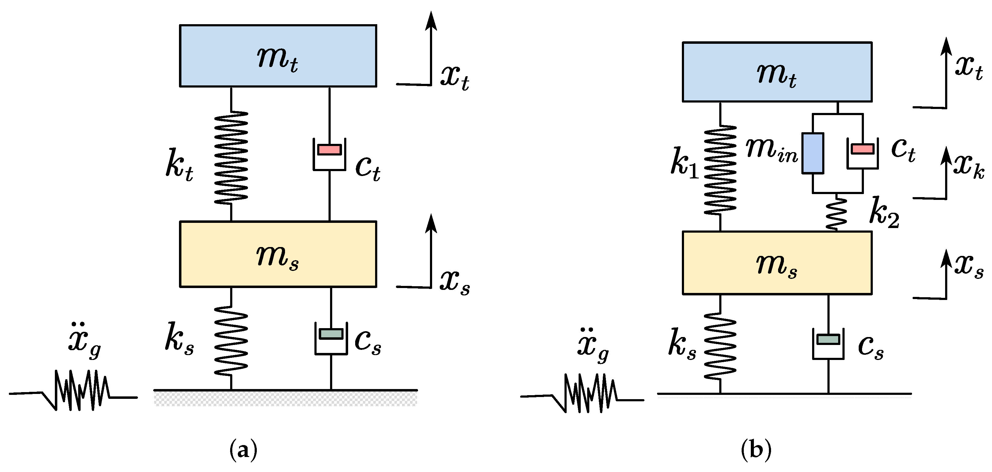
2.1. Numerical Model of SDOF System

The reaction forces of the spring and damping element are related to the relative displacement and velocity, respectively. While for the inerter element, the force magnitude is proportional to the relative acceleration between the endpoints. A typical ball-screw mechanical model of the ineter is presented in Figure 1. The force magnitude of the inerter can be noted as $F=m_{in}({\ddot{x}}_i-{\ddot{x}}_j)$, where the constant of proportionality $m_{in}$ is named as the inertance and has kilograms as units. Furthermore, the amount of energy it stores is equal to $1/2m_{in}({\dot{x}}_i^2-{\dot{x}}_j^2)$.

The mass, spring, and damper element make up the basic TMD, as shown in Figure 2a. However, when the inerter element is added, it can perform superior in terms of energy dissipation. In the real applications, the components of TMDI systems may also have more complex behavior. Thus, various mechanical topology layouts are put forward [23,37]. While in this paper, a typical linear model of TMDI is adopted to demonstrate the ability of inerter element, as shown in Figure 2b, which is mentioned in reference [38].

It is assumed that the whole system is excited by the base acceleration ${\ddot{x}}_g$, the equation of motion for the dynamic system indicated above could be obtained with the equilibrium of forces. Accordingly, the kinetic equations for both the TMD and TMDI are expressed in Equations (1) and (2), respectively.

$$\left[\begin{array}{cc}{m}_s& 0\\ 0& m_t\end{array}\right]\left[\begin{array}{c}{\ddot{x}}_s\hfill \\ {\ddot{x}}_t\hfill \end{array}\right]+\left[\begin{array}{cc}{c}_s+c_t& -c_t\\ -c_t& c_t\end{array}\right]\left[\begin{array}{c}{\dot{x}}_s\hfill \\ {\dot{x}}_t\hfill \end{array}\right]+\left[\begin{array}{cc}{k}_s+k_t& -k_t\\ -k_t& k_t\end{array}\right]\left[\begin{array}{c}{x}_s\hfill \\ x_t\hfill \end{array}\right]=-\left[\begin{array}{c}{m}_s\hfill \\ m_t\hfill \end{array}\right]{\ddot{x}}_g$$

(1)

$$\left[\begin{array}{ccc}{m}_s& 0& 0\\ 0& m_t+m_{in}& -m_{in}\\ 0& -m_{in}& m_{in}\end{array}\right]\left[\begin{array}{c}{\ddot{x}}_s\hfill \\ {\ddot{x}}_t\hfill \\ {\ddot{x}}_k\hfill \end{array}\right]+\left[\begin{array}{ccc}{c}_s& 0& 0\\ 0& c_t& -c_t\\ 0& -c_t& c_t\end{array}\right]\left[\begin{array}{c}{\dot{x}}_s\hfill \\ {\dot{x}}_t\hfill \\ {\dot{x}}_k\hfill \end{array}\right]+\left[\begin{array}{ccc}{k}_s+k_1+k_2& -k_1& -k_2\\ -k_1& k_1& 0\\ k_2& 0& k_2\end{array}\right]\left[\begin{array}{c}{x}_s\hfill \\ x_t\hfill \\ x_k\hfill \end{array}\right]=-\left[\begin{array}{c}{m}_s\\ m_t\\ 0\end{array}\right]{\ddot{x}}_g$$

(2)

where $m_s$, $k_s$, and $c_s$ are the mass, spring, and damping coefficient of the host structure; $m_t$, $c_t$ are the mass and damping of the addition attached damper; $m_{in}$ is the inertance of inerter element; $k_t$ is the spring stiffness of TMD; $k_1$, $k_2$ are the two spring stiffnesses of TMDI.

The transfer function (TF) reflects the output process of structural response under excitation, which presents the dynamic characteristics of the structure. As long as the transfer function of the structure is suppressed, the ideal control effect can be achieved regardless of the external excitation. For this reason, the optimization objective is to reduce the displacement transfer function of the main structure as much as possible. Meanwhile, in an effort to make the control effect more clearly reflected and representative, the parameters should be dimensionless. For this regard, the nondimensional expressions for the parameters listed above are expressed as follows:

$$\begin{array}{c}{\zeta }_s=c_s/\left(2m_s{\omega }_s\right),{\omega }_s=\sqrt{k_s/m_s},{\omega }_1=\sqrt{k_1/m_t},{\omega }_2=\sqrt{k_2/m_t},{\omega }_t=\sqrt{k_t/m_t},\hfill \\ {\zeta }_t=c_t/\left(2m_t{\omega }_t\right)=c_t/\left(2m_t{\omega }_1\right),u_t=m_t/m_s,u_{in}=m_{in}/m_t,\hfill \\ f_d={\omega }_t/{\omega }_s,f_1={\omega }_1/{\omega }_s,f_2={\omega }_2/{\omega }_s\hfill \end{array}$$

(3)

where ${\omega }_s,{\zeta }_s$ are the circular frequency and damping ratio of the primary structure; ${\omega }_1,{\omega }_2$ and ${\omega }_t$ are the circular frequency of spring $k_1$, $k_2$, and $k_t$, respectively; $u_t$ and $u_{in}$ are the mass ratio and interance-mass ratio; $\omega$ is the frequency of the external excitation; $f_1,f_2$, and $f_d$ represent the tuning frequency ratio of the spring $k_1,k_2$, and $k_t$ corresponding to the primary system.

Assuming that the base acceleration is simplified as a harmonic excitation, i.e., ${\ddot{x}}_g=e^{i\omega t}$, the displacement of the main structure can be denoted as $x_s=H_m\left(\omega \right)e^{i\omega t}$. Then, the dimensionless transfer function for the structural displacement ($H_m$) can be found in Equation (4). While the parameters of $A/B/C/D$ for TMD and TMDI can be obtained, as shown in Equations (5) and (6).

$$H_m\left(\beta \right)=\frac{x_s{\omega }_s^2}{{\ddot{x}}_g}=\left|\frac{A_i+B_i}{C_i+D_i}\right|$$

(4)

For TMD:

$$\left\{\begin{array}{c}{A}_1=u_t\left[{\beta }^2-f^2\left(1+u_t\right)\right]\hfill \\ B_1=2i{\zeta }_{t}f\beta u_t(u_t+1)\hfill \\ C_1=-u_t\left[{\beta }^2-{\beta }^4+f^2\left(-1+{\beta }^2\left(1+u_t\right)\right)+2i\beta \left(-f^2+p^2\right){\zeta }_s\right]\hfill \\ D_1=-2f\beta u_t{\zeta }_t\left[i\left(-1+{\beta }^2\left(1+u_t\right)\right)+2\beta {\zeta }_s\right]\hfill \end{array}\right.$$

(5)

For TMDI:

$$\left\{\begin{array}{c}{A}_2=-2f_2{\zeta }_t\beta {u_t}^2\left[-{\beta }^2+{f_1}^2\left(1+u_t\right)+{f_2}^2\left(1+u_t\right)\right]\hfill \\ B_2=-i{u_t}^2\left[-{\beta }^4{u}_{in}-{f_1}^2\left({f_2}^2-p^2{u}_{in}\right)\left(1+u_t\right)+{f_2}^2{\beta }^2\left(1+u_{in}+u_{in}{u}_t\right)\right]\hfill \\ C_2=-2f_2\beta {u_t}^2{\zeta }_t\left[\begin{array}{c}-2i\beta {\zeta }_s\left({f_1}^2+{f_2}^2-{\beta }^2\right)+{f_1}^2\left({\beta }^2(u_t+1)-1\right)\hfill \\ +{f_2}^2{\beta }^2{u}_t+{f_2}^2{\beta }^2-{f_2}^2-{\beta }^4+{\beta }^2\hfill \end{array}\right]\hfill \\ D_2=-{u_t}^2\left[i\left(\begin{array}{c}-{f_1}^2\left({\beta }^2(u_t+1)-1\right)\left({f_2}^2-{\beta }^2{u}_{in}\right)\hfill \\ +{f_2}^2{\beta }^2\left({\beta }^2(u_{in}{u}_t+u_{in}+1)-u_{in}-1\right)\hfill \\ -{\beta }^4\left({\beta }^2-1\right)u_{in}\hfill \end{array}\right)+2\beta {\zeta }_s\left(\begin{array}{c}{f_1}^2\left({\beta }^2{u}_{in}-{f_2}^2\right)\hfill \\ +{f_2}^2{\beta }^2(u_{in}+1)\hfill \\ -{\beta }^4{u}_{in}\hfill \end{array}\right)\right]\hfill \end{array}\right.$$

(6)

where $i=\sqrt{-1}$ is the imaginary number; $\beta =\omega /{\omega }_s$, which is the ratio between the frequency of base acceleration and main structure.

2.2. Parameters Optimization

The optimal design is needed to get the best performance of the dynamical vibration absorbers (DVAs). In the previous optimization of TMD, the fixed-point theory was commonly used [40]. For the undamped host structure, it is assumed that the transfer function curve always passes through a fixed point, when the damping ratio (${\zeta }_t$) changes only. By keeping the amplitude equal at the fixed point, the optimal tuning frequency of the device can be found. The optimal damping ratio is obtained by holding the curve at this fixed point until it reaches its peak. The analytical expression of the optimal parameters can be obtained through this method.

It is, however, incapable of handling a sophisticated model with more than three mechanical elements in the device. Furthermore, the damping ratio of the primary structure is ignored in this fixed-point theory, which does not correlate to reality. As a result, a general approach to solving these problems is required. The numerical searching method is performed, regarding peak relative displacement responses of the primary structure as the optimization objectives, which is indicated in the following expression.

$$\left\{\begin{array}{cc}\mathrm{Minimize}:& max\left(H_m\left(\beta \right)\right)\\ \mathrm{Objective}:& {\zeta }_{t,opt},f_{t,opt},f_{1,opt},f_{2,opt},u_{in,opt}\\ \mathrm{Subject}\mathrm{to}:& 0<{\zeta }_t,f_d,f_1,f_2,u_{in},u_t\le 1\end{array}\right.$$

(7)

These values are optimized in MATLAB software using the fmincon command [41] based on the above boundary conditions. Besides this, the damping ratios (${\zeta }_s$) for the primary structure are set as 0.01, 0.03, and 0.05 to give an example. The optimal parameters of TMD and TMDI with varied mass ratios ($u_t$) are obtained using this numerical method for various damping ratios (${\zeta }_s$) of the main structure, as illustrated in Figure 3 and Figure 4.

From the above figures, it can be seen that the damping ratio of the structure (${\zeta }_s$) affects the optimal design parameters of the DVA device. For both different devices, the value of ${\zeta }_d$ increased a little with the increase of ${\zeta }_s$, while $f_1$ and $f_d$ decreased with ${\zeta }_s$. In addition, as the mass ratio $u_t$ increases, the tuning frequency ratio of $f_d$ and $f_1$ decreases, while $f_2$ keeps rising when $u_t$ is less than 0.4 and then starts to fall. Meanwhile, the inertance – mass ratio ($u_{in}$) of TMDI has the same tendency as $f_2$. For convenience in practical application, all the results are fitted with the quartic polynomial, as written in Equation (8). In addition, the coefficient of the polynomial is reported in

Table 1. The coefficient of the polynomial for the optimal parameters.

		TMDI				TMD
		${\mathbf{u}}_{\mathbf{in}}$	${\mathbf{\zeta }}_{\mathbf{t}}$	${\mathbf{f}}_{\mathbf{1}}$	${\mathbf{f}}_{\mathbf{2}}$	${\mathbf{f}}_{\mathbf{d}}$	${\mathbf{\zeta }}_{\mathbf{t}}$
${\zeta }_s=0.01$	$p_1$	—1.969	—0.907	0.578	—1.800	0.220	—1.043
	$p_2$	5.114	2.606	—1.923	4.915	—0.746	2.708
	$p_3$	—4.832	—2.896	2.458	—4.981	1.138	—2.535
	$p_4$	1.855	1.485	—1.997	2.160	—1.269	1.389
	$p_5$	0.030	0.022	0.986	0.262	0.997	0.070
${\zeta }_s=0.03$	$p_1$	—1.547	—1.139	—0.403	—2.032	0.309	—1.022
	$p_2$	4.261	3.166	—0.133	5.379	—0.968	2.703
	$p_3$	—4.271	—3.394	1.407	—5.302	1.339	—2.543
	$p_4$	1.703	1.669	—1.806	2.249	—1.353	1.404
	$p_5$	0.043	0.006	0.962	0.251	0.990	0.073
${\zeta }_s=0.05$	$p_1$	—2.770	—1.404	1.982	—3.056	0.398	—0.981
	$p_2$	6.724	3.583	—5.619	7.908	—1.200	2.646
	$p_3$	—5.880	—3.596	5.567	—7.391	1.549	—2.507
	$p_4$	2.042	1.696	—2.955	2.891	—1.438	1.413
	$p_5$	0.039	0.012	1.009	0.191	0.983	0.074

.

$$P_{opt}\left(u_t\right)=p_1{u_t}^4+p_2{u_t}^3+p_3{u_t}^2+p_4{u}_t+p_5$$

(8)

2.3. Performance Comparison

To visually show the difference between the two oscillators, the displacement transfer functions of the main structure are plotted. The mass ratio $u_t$ for both TMD and TMDI is set as 0.10. The difference between them can be seen in Figure 5. Compared with the TMD, it could be found that the maximum amplitude with TMDI is significantly decreased. However, the TMDI has three peaks in its curve, which is one more than the TMD. This is because TMDI has three DOFs, as can be seen from the configuration, which means that there are more alternatives for adjusting the overall performance of device. In the process of functioning, the two springs of TMDI could play different roles. The spring $k_1$ is used for the primary tuning, while the spring $k_2$ is responsible for increasing the stroke and deformation between the damping element in order to absorbing more energy. As illustrated in Figure 6, the maximum amplitudes of the transfer function of the structural displacement at various mass ratios ($u_t$) are also compared. It can be observed that with the increasing of additional mass, the control effectiveness of the two devices improves, while the TMDI outperform the TMD.

What is more, the additional influence of the DVAs on the structure can be attributed to a higher damping ratio in the primary system. By comparing the altered damping ratio of the structure, the influence of the DVA on the structure can be explicitly represented. As for this respect, various methods are presented to evaluate the overall damping of a structure with the addition of dampers. As derived by reference [42], when the mass ratio is small enough, the equivalent damping ratio (${\xi }_e$) of the whole system can be estimated by comparing the amplitude of the transfer function, as described in Equation (9). In accordance with this method, the variation trend of the equivalent damping ratio of the whole system with different mass ratios is plotted in Figure 7, with an assumed damping ratio (${\zeta }_s$) of 0.03. It can be found that the equivalent damping ratio (${\zeta }_e$) of the system extended as the mass ratio $u_t$ increases. Compared to the TMD, the TMDI system could consume more energy with the assistance of inerter element.

$${\zeta }_e\approx \frac{1}{2H_{m,max}}$$

(9)

3. Case Study 1—A SDOF Oscillator

3.1. Parameters of SDOF Structure

In this section, an actual SDOF structure is adopted for time-domain analysis to evaluate the differences between two DVAs more intuitively. The mass of the structure is assumed to be 2000 kg, with a stiffness of 20,000 N/m and 379.47 $\mathrm{N}·\mathrm{m}/\mathrm{s}$ for the damping coefficient (${\zeta }_s=0.03$). In this section, the mass ratio $u_t$ for both TMD and TMDI are all set as 0.10. The specific values of each parameter can be obtained using Equation (8)), with the coefficients in Table 1. The parameters of the two equipments are listed in the table below.

3.2. Reaction of the Primary Structure

To compare the performance of the two devices, the typical ground motion records of EL Centro and Kobe waves are taken for verification. The reactions of the structure under seismic loading are obtained using the Newmark-$\beta$ algorithm [43], which is one of the most adopted time-integration methods [44,45]. The relative displacement and absolute acceleration of the main structure are depict in Figure 8 and Figure 9. It can be noticed that, for the same mass ratio, both devices perform well in the whole process. However, in comparison with the classical TMD, the TMDI can further decrease the response of the results over the entire time range.

3.3. Stroke of Damping elements

Apart from the responsiveness of the main structure, the stroke of devices is also the essential factor to consider. Especially in the buildings with limited space, the stroke of the additional devices is a critical restraint. In this SDOF system, the relative displacement is compared under different ground motions, as illustrated in Figure 10. In this regard, the TMD has the advantage of a shorter stroke, whereas the maximal relative displacement of the TMDI is around 1.3 times as much as the TMD. Additionally, the deformation of the two spring for the TMDI are also varied. The relative motion of $k_1$ is larger than $k_2$ because of smaller stiffness compared with the classical TMD. Whereas, the extra spring $k_2$ is utilized to increase the deformation of the damping element.

3.4. Energy Dissipation

As indicated in the

Table 2. Parameters of TMDI and TMD for the specific SDOF system.

	TMDI				TMD
${\mathit{m}}_{\mathit{t}}$(kg)	${\mathit{u}}_{\mathit{in}}$(kg)	${\mathit{c}}_{\mathit{t}}$(N·m/s)	${\mathit{k}}_{\mathit{1}}$(N/m)	${\mathit{k}}_{\mathbf{2}}$(N/m)	${\mathit{c}}_{\mathit{t}}$(Nm/s)	${\mathit{k}}_{\mathit{t}}$(N/m)
200.00	34.98	77.78	1272.47	372.24	214.15	1500.50

, the damping coefficient of TMDI is much smaller than that of TMD, which is around 1/3 of it. Therefore, a greater deformation is required to output larger damping forces to achieve the same desired energy dissipation. The damping forces and relative displacement for the damping element for each device are depicted in Figure 11 when activated by the earthquake. It can be seen that the hysteresis loops of the damping force and relative displacement for the TMD are broadly circular, whereas the curve of TMDI is almost elliptical. In contrast, the damping force of TMDI is much smaller, with a more extensive deformation compared with TMD.

The energy consumption curves of TMD and TMDI are given in Figure 12, with the example of EL Centro wave. It consumed about 538.74 and 568.64 kJ of energy for TMD and TMDI, accounting for 68.02% and 72.24% of the toltal energy harvest by the entire system, respectively. As can be observed, the TMDI could absorb more energy than the traditional TMD. At the same time, it is possible to select a damping element with a lower damping coefficient, hence reducing the requirements of the auxiliary device and cost. Similarly, a lower mass ratio of TMDI can be considered to achieve the same vibration suppression effectiveness.

4. Case Study 2– A MDOF Benchmark Model

4.1. Introduction of Model

In this section, a typical multi-story steel building located in Los Angeles is taken as a benchmark model [46] in this paper. It has commonly been used as a benchmark model to assess the effectiveness of various control strategies [47,48]. The planar dimensions of this structure are 30.48 m by 36.58 m, with a height of 80.77 m. There are 20 stories above the ground surface, and the roof denotes the 21st level, as depicted in Figure 13. It includes two extra basement floors, and each floor averages 3.96 m in elevation. The two basement floors have a height of 3.65 m, while the first floor has a height of 5.49 m. The horizontal displacement of the first floor is restricted by the concrete foundation walls and surrounding soil. The mass of the first and second floors is $2.66\times {10}^5$ kg and $2.83\times {10}^5$ kg, the mass of the third to 20th floors is $2.76\times {10}^5$ kg, and the mass of the roof is $2.92\times {10}^5$ kg. In this section, we only concentrate on the plane of this structure, as well as the short direction.

The structure is modeled as a plane-frame elements, and the mass and stiffness matrices for the structure are determined. There are 180 nodes interconnected by 284 elements in this model. The beam and column members are modeled as the plane element, with two nodes and six degrees of freedom. The detailed properties of these elements can be found in reference [49], including the length, area, the moment of inertia, modulus of elasticity, and mass density.

The structure is modelled by the finite element method (FEM), with 540 DOFs for the mass and stiffness matrix. After that, 14 DOFs on the first floor are eliminated, considering the boundary constraints on the bottom. In addition, the system can be further simplified because the floor slab can be assumed as rigid in the horizontal plane, and the nodes associated with each floor have the same horizontal displacement. Then the Guyan reduction method [50] is used to decrease the rotational and most of the vertical DOFs. In the end, the mass matrix ${\mathbf{M}}_s$ and stiffness matrix ${\mathbf{K}}_s$ have the dimensions $106\times 106$. The modal parameters, including the frequencies and mode shapes, are obtained by solving the following eigenvalue problem. The modal shapes of the first three modes are plotted in Figure 14.

$$\left({\mathbf{K}}_s-{\omega }^{\mathbf{2}}{\mathbf{M}}_s\right)\Phi =0$$

(10)

The damping matrix ${\mathbf{C}}_s$ is obtained on the base of the reduced system with the assumption of modal damping. The damping of each mode ${\zeta }_i$ is assumed to be proportional to the associated frequency, with a maximum critical damping of 10%. Then, the values of ${\zeta }_i$ are calculated according to Equation (11), and the global damping matrix can be acquired as in Equation (12).

$${\zeta }_i=\min \left\{{\displaystyle \frac{{\omega }_i}{50{\omega }_1}},0.1\right\}.$$

(11)

$${\mathbf{C}}_s={\mathbf{M}}_s\Phi \left(2\zeta \omega \right){\Phi }^{-1}$$

(12)

where ${\omega }_i$ and ${\zeta }_i$ are the $i_{th}$ modal circular frequency and damping ratio of the structure, respectively; $\zeta =diag\{{\zeta }_1,{\zeta }_2,\cdots ,{\zeta }_n\}$; $\omega =diag\{{\omega }_1,{\omega }_2,\cdots ,{\omega }_n\}$.

4.2. External Loads Acting on the Structure

In order to further verify the dynamic performance of the high–rise buildings with the designed proposed control strategy. It is supposed that this structure is excited by the earthquake. In addition, it is assumed that the base accleration excitation is non–stationary in nature and has a more complicated spectral content than the white–noise random process. In this respect, the colored power spectral density (PSD) of the Clough–Penzien model [51] is employed as the base excitation, which is represented as shown in Equation (13). According to the theory of earthquake engeering, the amplitude of ground motion is filtered by the soil when it originates at the bed rocket. The soil effect could be converted to a two DOF linear filter that filters out the low-frequency component.

$$S_{{\ddot{x}}_g}\left(\omega \right)=S_0\frac{{\omega }_g^4+4{\zeta }_g^2{\omega }_g^2{\omega }^2}{{\left({\omega }_g^2-{\omega }^2\right)}^2+4{\zeta }_g^2{\omega }_g^2{\omega }^2}\frac{{\omega }^4}{{\left({\omega }_f^2-{\omega }^2\right)}^2+4{\zeta }_f^2{\omega }_f^2{\omega }^2}$$

(13)

where $S_0$ is a scale factor; ${\zeta }_g$, ${\omega }_g$ denote the equivalent damping ratio and fundamental frequency of the single-layer soil of the local site; ${\zeta }_f$, ${\omega }_f$ denote the equivalent damping ratio and fundamental frequency of the second-layer soil of the local site.

In the power spectral density (PSD), the values of the parameters considering different types of soils are indicated in

Table 3. The parameters of the Clough–Penzien model for different soil types.

Soil Type	${\mathit{\omega }}_{\mathit{g}}$ (rad/s)	${\mathit{\zeta }}_{\mathit{g}}$	${\mathit{\omega }}_{\mathit{f}}$ (rad/s)	${\mathit{\zeta }}_{\mathit{f}}$
Firm	15.0	0.6	1.5	0.6
Medium	10.0	0.4	1.0	0.6
Soft	5.0	0.2	0.5	0.6

, as illustrated in reference [51]. The short period of ground motion is related to the firm soil site, while the long period of ground motion refers to the soft soil site. The structure is considered to be at the firm soil site in this region, for the reason that the response would be more severe with the short period of base excitation. The scale factor $S_0$ demonstrated in Equation (13) is considered as 1 $g^2·s$, while other parameters are selected from Table 3 according to the firm soil type. After that, the base acceleration excitation is a non-stationary random process specified by the Clough–Penzien spectra. Three authentic acceleration signals are then generated in accordance with this PSD model and the use of inverse Fourier transformation, which is named W1 ∼ W3.

Moreover, the efficacy of the two DVAs is tested with the actual ground motions. The construction is assumed to be placed on a class ${\mathrm{I}}_1$ site with firm soils in the second group, according to the Chinese standard code for seismic design of buildings [52]. The shear velocity $v_{s20}$ is 500∼800 m/s for the firm soil site, which is transformed to 510∼760 m/s for $v_{s30}$ according to the standard of ASCE [53]. Following that, the target acceleration response spectra are obtained, as shown in Figure 15. Seven records are obtained from the database of PEER [54], and the selected ground motion data are listed in

Table 4. The information of the selected earthquake records.

Series	Earthquake Name	Year	Magnitude	Station Name	${\mathit{V}}_{\mathit{s}30}$ (m/s)	${\mathit{R}}_{\mathit{jb}}$ (km)
R1	Chi-Chi_Taiwan	1999	7.62	CHY019	573.04	46.59
R2	Chi-Chi_Taiwan	1999	7.62	HWA035	677.49	44.02
R3	Chi-Chi_Taiwan	1999	7.62	ILA050	621.06	63.82
R4	Chi-Chi_Taiwan	1999	7.62	TCU071	624.85	0.00
R5	Chi-Chi_Taiwan	1999	7.62	TCU089	535.13	83.38
R6	Chi-Chi_Taiwan	1999	7.62	TTN051	665.20	30.77
R7	Chi-Chi_Taiwan	1999	7.62	TCU129	511.18	1.83

. After that, the response spectrum for all the ground motions are also plotted in Figure 15.

4.3. Dynamic Modal Establishment for Passive Control

In the previous study, it is normally organized at the top of the structure if only a single tuned-type oscillator is considered [32]. The first-order frequency of the structure is mainly considered for the single TMDI to achieve the best control effect. However, this usually causes some problems. The mass and volume of the device will be so large that the structure needs to be specially designed to consider the arrangement of the attached device, which may result in additional construction and costs. For this reason, in this section, multiple TMD and TMDIs are considered to be arranged in the structure to reduce the huge additional mass of a single device. Besides, the designed frequency of each DVA is adjusted to control to enhance the resilience and dependability of the equipment.

When considering the arrangement of DVAs, it can be considered according to the distribution of vibration shapes for different modes. From Figure 14, it can be found that the largest amplitude of the fundamental mode is at the top of the building, whereas the peak position of the second mode is on the ninth floor. According to this, multiple DVAs are employed to suppress the first two modes of the structure. Then, eight devices are organized in this section, and they are located between the 7th and 21st floors, with intervals of two stories. The schematic of the entire system is shown in Figure 16. In addition, the frequencies are uniformly dispersed from the first to the second model, with the frequency for each device computed using Equation (14). At the same time, the other parameters can be acquired by Equation (8) when the frequency is definite.

$${\omega }_{t,i}={\omega }_{s,1}+\frac{{\omega }_{s,2}-{\omega }_{s,1}}{n_t-1}\left(i-1\right)\left(i=1,2,\cdots ,n_t\right)$$

(14)

where ${\omega }_{s,1}$ and ${\omega }_{s,2}$ are the fundamental and second model frequency of the main structure, respectively; ${\omega }_{t,i}$ is the frequency that the $i_{th}$ TMD and TMDI need to be controlled; $n_t$ is the total number of DVAs.

When the parameters of each device are determined, the equation of motion of the whole system under the base acceleration excitation is expressed as in the following formulation.

$$\mathbf{M}\ddot{\mathbf{X}}+\mathbf{C}\dot{\mathbf{X}}+\mathbf{KX}=-\mathbf{ML}{\ddot{x}}_g$$

(15)

For the multiple TMDs:

$$\mathbf{M}=\left[\begin{array}{cc}{\mathbf{M}}_{\mathbf{S}}& \mathbf{0}\\ \mathbf{0}& {\mathbf{M}}_{\mathbf{t}}\end{array}\right],\mathbf{C}=\left[\begin{array}{cc}{\mathbf{C}}_{\mathbf{S}}+{\mathbf{P}}_1{\mathbf{C}}_{\mathbf{t}}{{\mathbf{P}}_1}^{\mathrm{T}}& -{\mathbf{P}}_1{\mathbf{C}}_{\mathbf{t}}\\ -{\mathbf{C}}_{\mathbf{t}}{{\mathbf{P}}_1}^{\mathrm{T}}& {\mathbf{C}}_{\mathbf{t}}\end{array}\right],\mathbf{K}=\left[\begin{array}{cc}{\mathbf{K}}_{\mathbf{S}}+{\mathbf{P}}_1{\mathbf{K}}_{\mathbf{t}}{{\mathbf{P}}_1}^{\mathrm{T}}& -{\mathbf{P}}_1{\mathbf{K}}_{\mathbf{t}}\\ -{\mathbf{K}}_{\mathbf{t}}{{\mathbf{P}}_1}^{\mathrm{T}}& {\mathbf{K}}_{\mathbf{t}}\end{array}\right]$$

(16)

For the multiple TMDIs:

$$\begin{array}{c}\mathbf{M}=\left[\begin{array}{ccc}{\mathbf{M}}_{\mathbf{s}}& \mathbf{0}& \mathbf{0}\\ \mathbf{0}& {\mathbf{M}}_{\mathbf{t}}+{\mathbf{M}}_{\mathbf{in}}& -{\mathbf{M}}_{\mathbf{in}}\\ \mathbf{0}& -{\mathbf{M}}_{\mathbf{in}}& {\mathbf{M}}_{\mathbf{in}}\end{array}\right],\mathbf{C}=\left[\begin{array}{ccc}{\mathbf{C}}_{\mathbf{s}}& \mathbf{0}& \mathbf{0}\\ \mathbf{0}& {\mathbf{C}}_{\mathbf{t}}& -{\mathbf{C}}_{\mathbf{t}}\\ \mathbf{0}& -{\mathbf{C}}_{\mathbf{t}}& {\mathbf{C}}_{\mathbf{t}}\end{array}\right]\hfill \\ \mathbf{K}=\left[\begin{array}{ccc}{\mathbf{K}}_{\mathbf{s}}+{\mathbf{P}}_2\left({\mathbf{K}}_{\mathbf{1}}+{\mathbf{K}}_{\mathbf{2}}\right){{\mathbf{P}}_2}^{\mathbf{T}}& -{\mathbf{P}}_2{\mathbf{K}}_{\mathbf{1}}& -{\mathbf{P}}_2{\mathbf{K}}_{\mathbf{2}}\\ -{\mathbf{K}}_{\mathbf{1}}{{\mathbf{P}}_2}^{\mathbf{T}}& {\mathbf{K}}_{\mathbf{1}}& \mathbf{0}\\ -{\mathbf{K}}_{\mathbf{2}}{{\mathbf{P}}_2}^{\mathbf{T}}& \mathbf{0}& {\mathbf{K}}_{\mathbf{2}}\end{array}\right]\hfill \end{array}$$

(17)

where $\ddot{\mathbf{X}},\dot{\mathbf{X}}$ and $\mathbf{X}$ are the relative acceleration, velocity, and displacement of the global system; $\mathbf{M}$, $\mathbf{C}$ and $\mathbf{K}$ are the mass, stiffness, and damping matrix of the whole system, respectively; ${\mathbf{M}}_{\mathbf{s}}$, ${\mathbf{C}}_{\mathbf{s}}$ and ${\mathbf{K}}_{\mathbf{s}}$ are the mass, stiffness, and damping matrix of the original main system, respectively; ${\mathbf{M}}_{\mathbf{t}}=diag\{m_{t1},m_{t2},\cdots ,m_{tn}\}$ is the diagonal matrix of additional mass of TMD and TMDI; ${\mathbf{M}}_{\mathbf{in}}=diag\{m_{in1},m_{in2},\cdots ,m_{inn}\}$ is the diagonal matrix of inerterance; ${\mathbf{C}}_{\mathbf{t}}=diag\{c_{t1},c_{t2},\cdots ,c_{tn}\}$ is the diagonal matrix of damping of TMD and TMDI; ${\mathbf{K}}_{\mathbf{1}}=diag\{k_{11},k_{12},\cdots ,k_{1n}\}$ is the diagonal matrix of spring $k_1$ of TMDI; ${\mathbf{K}}_{\mathbf{2}}=diag\{k_{21},k_{22},\cdots ,k_{2n}\}$ is the diagonal matrix of spring $k_2$ of TMDI; ${\mathbf{K}}_{\mathbf{t}}=diag\{k_{t1},k_{t2},\cdots ,k_{2tn}\}$ is the diagonal matrix of spring $k_t$ of TMD; ${\mathbf{P}}_{\mathbf{1}}$ and ${\mathbf{P}}_{\mathbf{2}}$ are the Boolean matrix for the location of TMD and TMDI, respectively; $\mathbf{L}$ is the distribution matrix for the inertia forces under earthquake; $n_s$ is the total number of DOFs of the original structure; ${\ddot{x}}_g$ is the acceleration of ground motion.

4.4. Active Control with Multiple DVAs

Passive control does not require external energy and can maintain process stability. However, some shortages of the passive control strategy exist in the operation period, such as start-up lag and large stroke. While the active control method is a useful technique in addressing such issues, which have been frequently employed in practice. To implement the effective control, multiple active TMDs and TMDIs are adopted in this section. The placement is identical to that of passive control, with the exception of the addition of an active actuator between each additional mass of devices and the main structure, as shown in Figure 16. Consequently, the equation of motion for the entire system has altered as a result of the inclusion of active forces, as illustrated in the equation below.

$$\mathbf{M}\ddot{\mathbf{X}}+\mathbf{C}\dot{\mathbf{X}}+\mathbf{KX}=-\mathbf{ML}{\ddot{x}}_g+{\mathbf{B}}_s{\mathbf{U}}_e$$

(18)

where ${\mathbf{U}}_e$ is the external active forces; ${\mathbf{B}}_s$ is the Boolean matrix of the active force distribution in global coordinates.

When the actuator is added, the challenge of determining how to design the actuator output forces should be examined. In this part, the design method is based on the linear quadratic regulator (LQR) [55]. Firstly, the equation of motion can be transformed into the form of state space, as shown in Equation (19). Furthermore, for the sake of computation, it is assumed that the displacements and accelerations are measurable for all the DOFs.

$$\left\{\begin{array}{c}\dot{\mathbf{Z}}\left(t\right)=\mathbf{AZ}\left(t\right)+\mathbf{BU}\left(t\right)+\mathbf{D}{\ddot{x}}_g\hfill \\ \mathbf{Y}\left(t\right)=\mathbf{CZ}\left(t\right)+\mathbf{H}{\ddot{x}}_g\hfill \end{array}\right.$$

(19)

$$\begin{array}{c}\mathbf{A}=\left[\begin{array}{cc}\mathbf{0}& \mathbf{I}\\ -{\mathbf{M}}^{-1}\mathbf{K}& -{\mathbf{M}}^{-1}\mathbf{C}\end{array}\right],\mathbf{B}=\left[\begin{array}{c}\mathbf{0}\\ {\mathbf{M}}^{-1}{\mathbf{B}}_{\mathbf{s}}\end{array}\right],\mathbf{D}=\left[\begin{array}{c}\mathbf{0}\\ \mathbf{L}\end{array}\right],\hfill \\ \mathbf{C}=\left[\begin{array}{cc}\mathbf{I}& \mathbf{0}\\ -{\mathbf{M}}^{-1}\mathbf{K}& -{\mathbf{M}}^{-1}\mathbf{C}\end{array}\right],\mathbf{H}=\left[\begin{array}{c}\mathbf{0}\hfill \\ \mathbf{L}\hfill \end{array}\right]\hfill \end{array}$$

(20)

where $\mathbf{Z}={\left\{\mathbf{X},\dot{\mathbf{X}}\right\}}^{\mathrm{T}}$ is the state response of the whole system.

After that, the control objective is to satisfy a quadratic performance generalization, as indicated in Equation (21). In addition, the optimal control force $\mathbf{U}$ can be expressed as a function of the state of system $\mathbf{Z}$, as presented in Equation (21).

$$J=\frac{1}{2}{\int }_{t_0}^{\infty }\left[{\mathbf{Z}}^T\left(t\right)\mathbf{QZ}\left(t\right)+{\mathbf{U}}^T\left(t\right)\mathbf{RU}\left(t\right)\right]dt$$

(21)

$$\mathbf{U}\left(t\right)=\mathbf{GZ}\left(t\right)$$

(22)

where $\mathbf{Q}$ and $\mathbf{R}$ are the weight matrices of the structural state response and the output forces, and they are semi-positive and positive definite matrices, respectively; $\mathbf{G}$ is the optimal state feedback gain matrix.

The weights matrix of $\mathbf{Q}$ is presumed to be a function of the mass and stiffness matrices of the whole system. While the weights matrix $\mathbf{R}$ for the active force is assumed to be the identity matrix, as shown in Equation (23). The weight coefficient of $\alpha$ and $\beta$ are assumed to be ${10}^3$ and ${10}^{-3}$ through constant trial, respectively, and it can also be modified according to actual needs. According to stochastic control theory, the optimal feedback force gain $\mathbf{G}$ can be obtained by solving the Riccati matrix algebraic equation [55], as demonstrated in Equations (24) and (25).

$$\mathbf{Q}=\alpha \left[\begin{array}{cc}\mathbf{M}& \mathbf{0}\\ \mathbf{0}& \mathbf{K}\end{array}\right],\mathbf{R}=\beta \mathbf{I}$$

(23)

$$-\mathbf{PA}-{\mathbf{A}}^{\mathbf{T}}\mathbf{P}+\mathbf{PB}{\mathbf{R}}^{-\mathbf{1}}{\mathbf{B}}^{\mathbf{T}}\mathbf{P}-\mathbf{Q}=\mathbf{0}$$

(24)

$$\mathbf{G}={\mathbf{R}}^{-1}{\mathbf{B}}^{\mathrm{T}}\mathbf{P}$$

(25)

5. Verification for Vibration Suppression

The time histories under the specified ground motion are estimated using the Newmark-$\beta$ method, based on the benchmark model stated in the preceding section and the control strategy. In this case, eight TMDs and TMDIs are organized in accordance with Figure 16, with a mass of 21.783 t for each device, assuming a total mass of 3% of the main structure. The remaining spring stiffness and damping coefficient are determined using the approach described in Section 2.2. The results of both the passive and active control systems have been computed and are presented in this section.

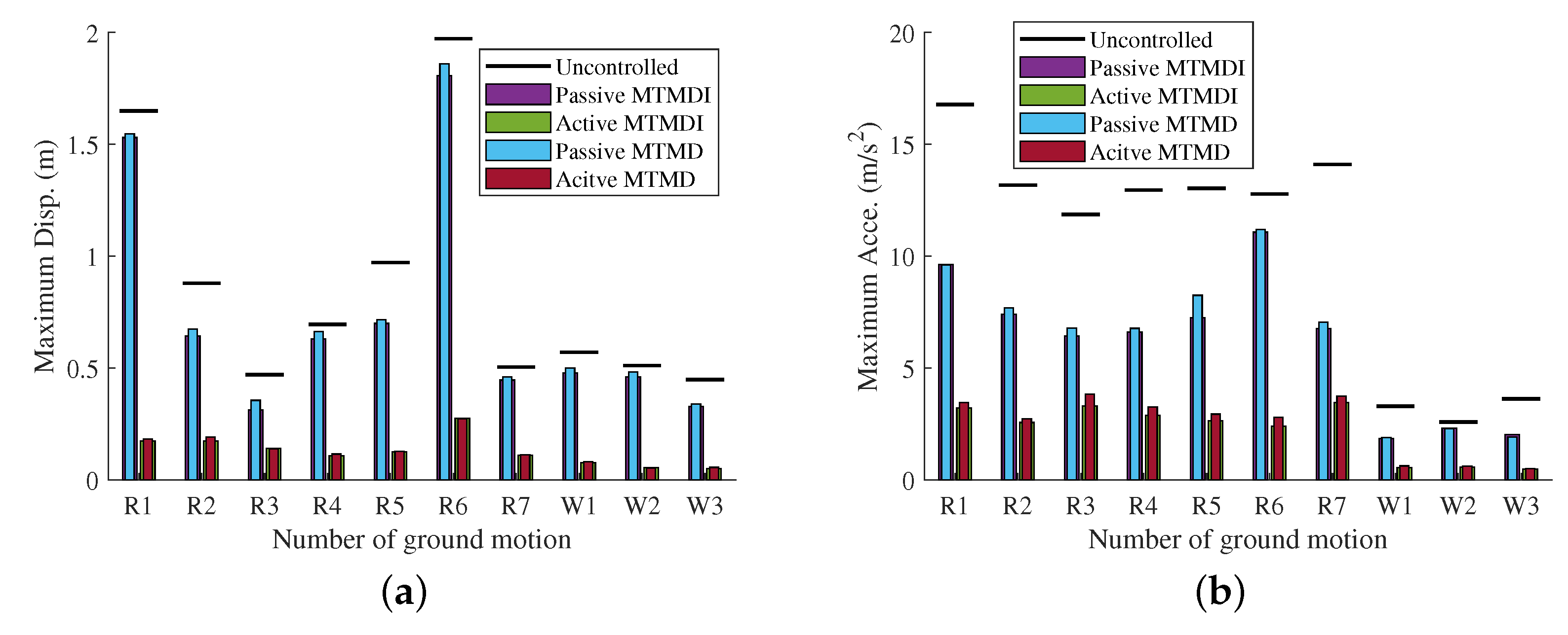
5.1. The Top Response of This Building

Under external excitation, the reaction of the top of this high-rise building is the prominent factor that needs to be taken into account. By adopting parameters designed according to the proposed passive and active method, a series of time history analyses were conducted for verification. Taking the ground motion data of R2 as an example, as can be seen in Table 4, the response of the building is plotted, as shown in Figure 17. When the seismic acted, it can be seen that the structural response under passive control is reduced, but there is still great potential for the improvement of mitigation effectiveness. Meanwhile, it can be found that TMDI can further improve the suppression effect during the earthquake with the same mass ratio. In addition, the application of active control can drastically diminish the responsiveness of the structure, compared with the passive control methods.

In addition, the PSD of the top structural response is plotted to assess differences in the frequency domain, as shown in Figure 18. It can be observed that, except for the fundamental mode, higher–order modes also have the impacts on the displacement and acceleration response of the structure under the uncontrolled cases. The passive control mainly affects the first- and second-order structure modes but has limited influence on the remainder of the higher-order modes. However, the active control performs better, with reduced frequency sensitivity and significant suppression of all modes. This shows that active control features the strength of being less sensitive to excitation and that it can still provide effective control forces in situations where the external input is varied.

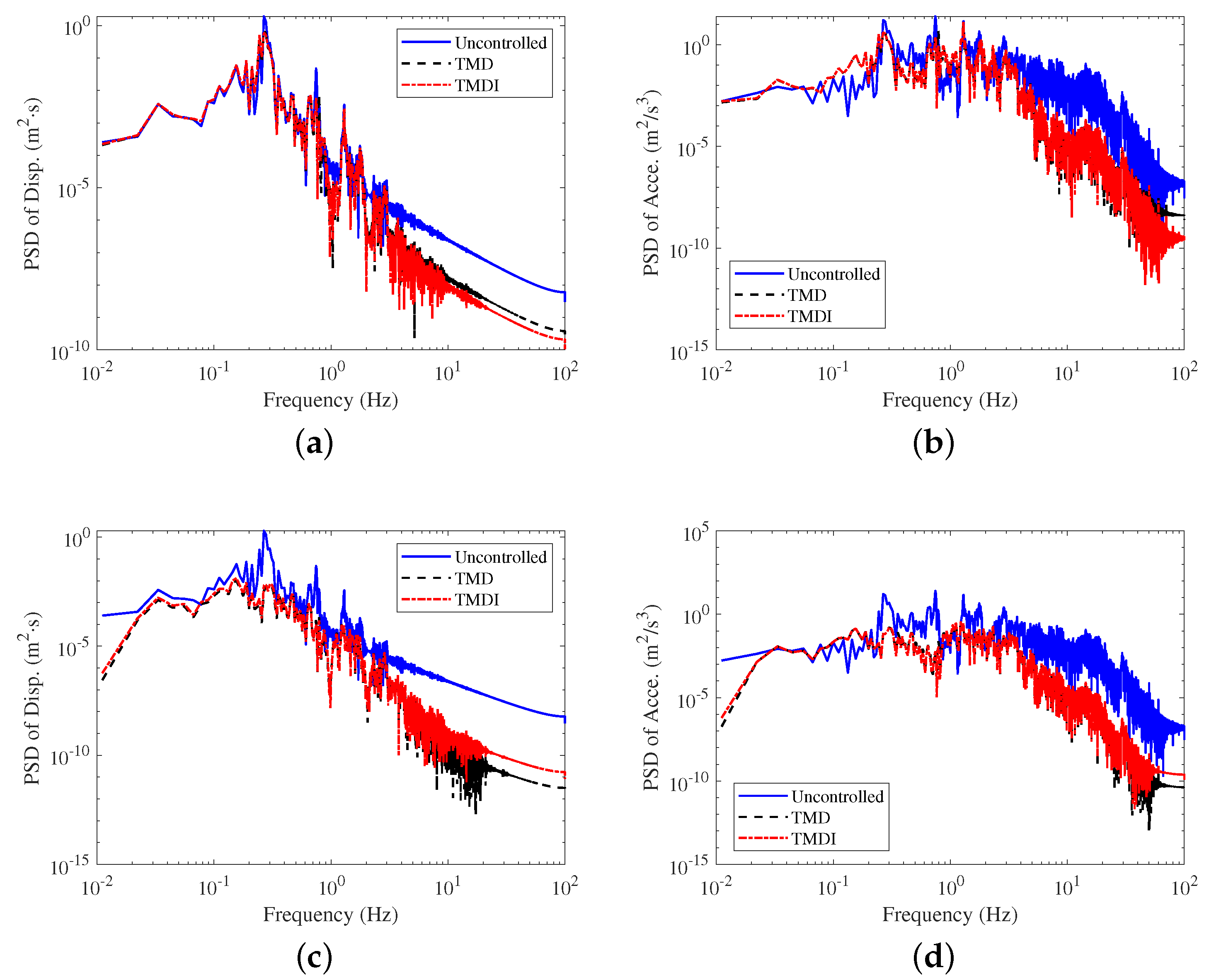
5.2. Statistical Characteristics of the Response

The time-dependent reaction shown above is the consequence of assuming the structure is in the undamaged condition. After a system is subjected to a strong earthquake, some non–structural components may be damaged and no longer be able to offer auxiliary stiffness to the structure, resulting in stiffness decline. Considering this situation, the stiffness of the structure is discounted in this situation for the further analysis, and it is supposed to be 0.9 times that of the undamaged condition. Figure 19 and Figure 20 compare the maximum amplitude of the structural response before and after being damage under various ground motions. It can be seen that the amplitude of the main structure decreased after the structure got damaged. This could be resulted by the extension of structural period. With approximately constant mass, the reduction in stiffness causes a reduction in the frequency of the structure, resulting in a longer period. Then the structure will capture less energy, resulting in smaller responses, as demonstrated in Figure 14.

When the stiffness of the structure declined, the control effects of TMDI and TMD in the passive state deteriorated considerably, because the parameter of DVAs are designed based on the structural frequencies before being damaged. As for the passive control strategy, the counterproductive result could happen in some cases, as shown in Figure 20a. The amplitude is amplified compared with the uncontrolled situation. Although some reduction in vibration can be achieved with passive control, there is still much to be done to improve the performance. The efficacy of the multiple active TMDI (MATMDI) is more stable than the given multiple active TMD (MATMD), and the reaction of the structure is always kept as low as possible for the given ground motion data.

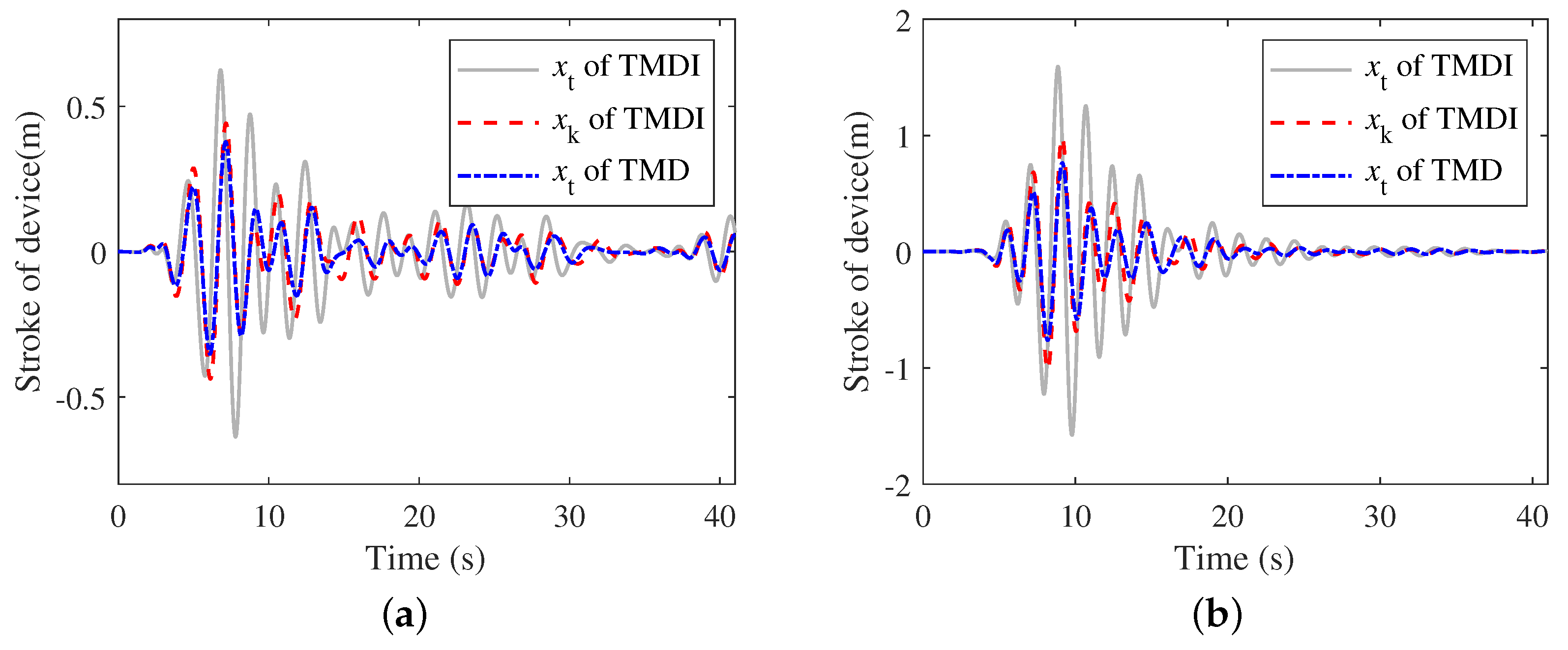
5.3. Stroke of the Devices

The amplitude of the stroke of every DVA is additionally an essential aspect to consider. The outcomes of identifying the maximum relative displacement per device in terms of each floor movement are obtained. And the records under all the ground motions are count out throught the box–plot, as depicted in Figure 21. Before the structure got damaged, the stroke of the device could be significantly reduced under active control compared to passive control. In most cases, the relative motion of MATDMI increased compared with MATMD in order to achieve the superior vibration mitigation effects. However, after the structure being damaged, the stiffness of the structure decreased. The frequencies of some devices altered in the passive control mode, making it difficult to resonate with the host structure. Then the stroke of devices have been reduced.

Additionally, because of the first mode that the devices controlled, the stroke of the first device is the greatest in passive control strategy, and the value of the second to the fifth device steadily diminishes. While the stroke of the sixth to eighth devices increased at the same time, due to the location close to the peak position of the second mode shape. In the active control, the relative movements significantly decreased, particularly for the foremost device, and the lower position the device located, the smaller the strokes it makes. This once again highlights the value of active control and is not sensitive to the structural variation.

6. Conclusions

In this study, a dynamic vibration absorber is integrated with a traditional TMD by adding an inerter element. According to the quantity and features of the various mechanical elements, a simple and effective topology of the system is adopted. To address the shortcomings of the classical fixed-point theory, the optimal design parameters of the TMDI are calculated for the damped SDOF system under the base acceleration by using the numerical optimization method. Moreover, the variation between the conventional TMD and TMDI are compared in the frequency and time domains. On this basis, an actual multi-story steel structure model is used to test the mitigation effect of TMDI under severe earthquakes. In addition, multiple passive and active control strategies of TMDI are proposed, considering the distribution characteristics of the structure. The effectiveness of vibration suppression is verified through time history analysis. From the results, some conclusions can be drawn as follows.

1.

The deficiency of classical fixed-point theory can be compensated by employing numerical searching, and the optimal design parameters of TMD and TMDI under external excitation can be effectively found.

2.

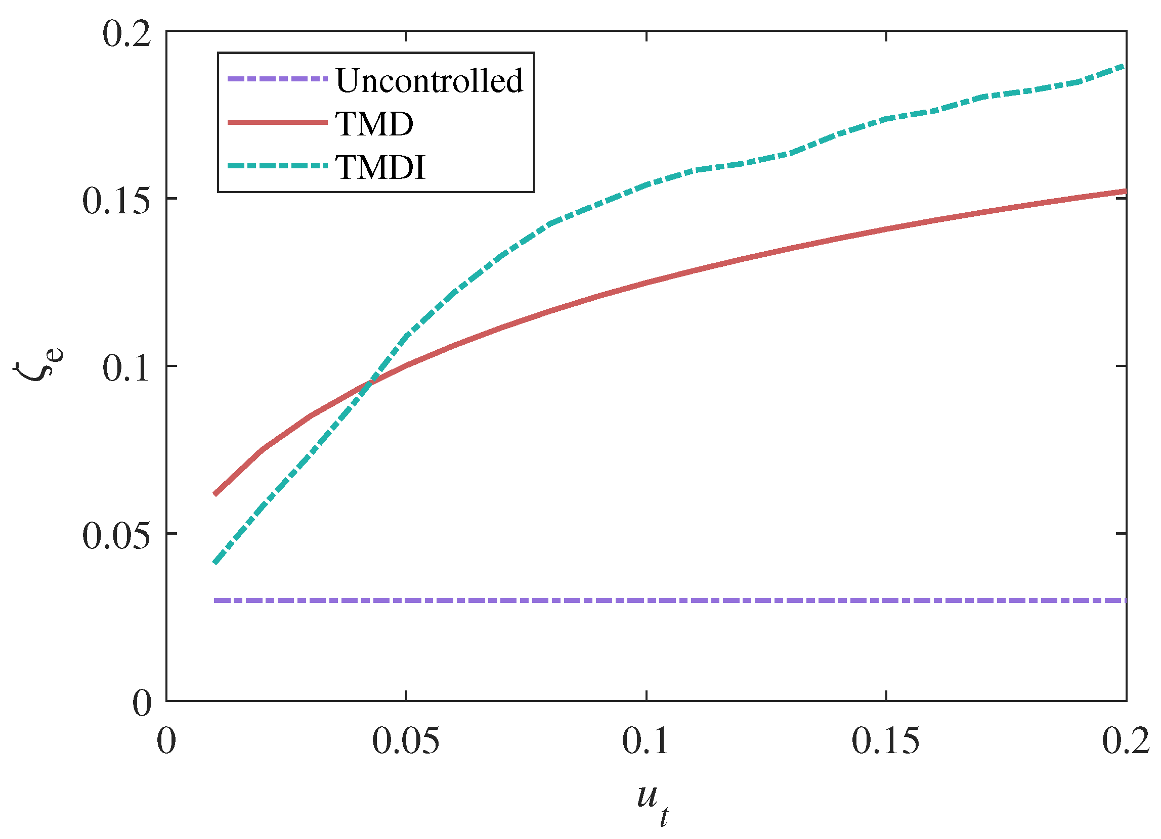
The TMDI performs better than the classical TMD, with the lower amplitude of the transfer function for the primary system. Meanwhile, the TMDI can provide more extra additional damping to the structure and increase the overall system energy dissipation, but the stroke has to be increased.

3.

With the contribution of extra actuators, the multiple active TMDI could greatly alleviate the response of the structure and stroke of attached DVAs. Besides, it also has the strength of being insensitive to structural and environmental changes, with stronger robustness and stability.

References

1. Ismail, M. Seismic isolation of structures. Part I: Concept, review and a recent development. Hormigón Acero 2018, 69, 147–161. [Google Scholar] [CrossRef]
2. Zhou, Y.; Shao, H.; Cao, Y.; Lui, E.M. Application of buckling-restrained braces to earthquake-resistant design of buildings: A review. Eng. Struct. 2021, 246, 112991. [Google Scholar] [CrossRef]
3. De Domenico, D.; Ricciardi, G.; Takewaki, I. Design strategies of viscous dampers for seismic protection of building structures: A review. Soil Dyn. Earthq. Eng. 2019, 118, 144–165. [Google Scholar] [CrossRef]
4. Elias, S.; Matsagar, V. Research developments in vibration control of structures using passive tuned mass dampers. Annu. Rev. Control 2017, 44, 129–156. [Google Scholar] [CrossRef]
5. Haskett, T.; Breukelman, B.; Robinson, J.; Kottelenberg, J. Tuned Mass Dampers under Excessive Structural Excitation; Report; Motioneering Inc.: Guelph, ON, Canada, 2004. [Google Scholar]
6. McNamara, R.J. Tuned mass dampers for buildings. J. Struct. Div. 1977, 103, 1785–1798. [Google Scholar] [CrossRef]
7. Kwok, K.C. Damping increase in building with tuned mass damper. J. Eng. Mech. 1984, 110, 1645–1649. [Google Scholar] [CrossRef]
8. Lu, X.; Chen, J. Parameter optimization and structural design of tuned mass damper for Shanghai centre tower. Struct. Des. Tall Spec. Build. 2011, 20, 453–471. [Google Scholar] [CrossRef]
9. Yang, F.; Sedaghati, R.; Esmailzadeh, E. Vibration suppression of structures using tuned mass damper technology: A state-of-the-art review. J. Vib. Control 2021, 28, 812–836. [Google Scholar] [CrossRef]
10. Rahimi, F.; Aghayari, R.; Samali, B. Application of tuned mass dampers for structural vibration control: A state-of-the-art review. Civ. Eng. J. 2020, 6, 1622–1651. [Google Scholar] [CrossRef]
11. Den Hartog, J.P. Mechanical Vibrations; Courier Corporation: North Chelmsford, MA, USA, 1985. [Google Scholar]
12. Warburton, G.B. Optimum absorber parameters for various combinations of response and excitation parameters. Earthq. Eng. Struct. Dyn. 1982, 10, 381–401. [Google Scholar] [CrossRef]
13. Asami, T.; Nishihara, O.; Baz, A.M. Analytical solutions to H and H2 optimization of dynamic vibration absorbers attached to damped linear systems. J. Vib. Acoust. 2002, 124, 284–295. [Google Scholar] [CrossRef]
14. Hoang, N.; Warnitchai, P. Design of multiple tuned mass dampers by using a numerical optimizer. Earthq. Eng. Struct. Dyn. 2005, 34, 125–144. [Google Scholar] [CrossRef]
15. Nishihara, O.; Asami, T. Closed-form solutions to the exact optimizations of dynamic vibration absorbers (minimizations of the maximum amplitude magnification factors). J. Vib. Acoust. 2002, 124, 576–582. [Google Scholar] [CrossRef]
16. Li, C.; Liu, Y. Optimum multiple tuned mass dampers for structures under the ground acceleration based on the uniform distribution of system parameters. Earthq. Eng. Struct. Dyn. 2003, 32, 671–690. [Google Scholar] [CrossRef]
17. Elias, S.; Matsagar, V.; Datta, T. Effectiveness of distributed tuned mass dampers for multi-mode control of chimney under earthquakes. Eng. Struct. 2016, 124, 1–16. [Google Scholar] [CrossRef]
18. Vaiana, N.; Sessa, S.; Marmo, F.; Rosati, L. A class of uniaxial phenomenological models for simulating hysteretic phenomena in rate-independent mechanical systems and materials. Nonlinear Dyn. 2018, 93, 1647–1669. [Google Scholar] [CrossRef]
19. Vaiana, N.; Sessa, S.; Rosati, L. A generalized class of uniaxial rate-independent models for simulating asymmetric mechanical hysteresis phenomena. Mech. Syst. Signal Process. 2021, 146, 106984. [Google Scholar] [CrossRef]
20. Zhang, M.; Xu, F. Tuned mass damper for self-excited vibration control: Optimization involving nonlinear aeroelastic effect. J. Wind Eng. Ind. Aerodyn. 2022, 220, 104836. [Google Scholar] [CrossRef]
21. Chen, X.; Kareem, A.; Xu, G.; Wang, H.; Sun, Y.; Hu, L. Optimal tuned mass dampers for wind turbines using a Sigmoid satisfaction function-based multiobjective optimization during earthquakes. Wind Energy 2021, 24, 1140–1155. [Google Scholar] [CrossRef]
22. Tseng, H.E.; Hrovat, D. State of the art survey: Active and semi-active suspension control. Veh. Syst. Dyn. 2015, 53, 1034–1062. [Google Scholar] [CrossRef]
23. Ma, R.; Bi, K.; Hao, H. Inerter-based structural vibration control: A state-of-the-art review. Eng. Struct. 2021, 243, 112655. [Google Scholar] [CrossRef]
24. Smith, M.C. The inerter: A retrospective. Annu. Rev. Control. Robot. Auton. Syst. 2020, 3, 361–391. [Google Scholar] [CrossRef]
25. Makris, N.; Kampas, G. Seismic protection of structures with supplemental rotational inertia. J. Eng. Mech. 2016, 142, 4016089. [Google Scholar] [CrossRef]
26. Smith, M.C.; Houghton, N.E.; Long, P.J.; Glover, A.R. Force-Controlling Hydraulic Device. US Patent 8,881,876, 11 November 2014. [Google Scholar]
27. Luo, Y.; Sun, H.; Wang, X.; Chen, A.; Zuo, L. Parametric optimization of electromagnetic tuned inerter damper for structural vibration suppression. Struct. Control Health Monit. 2021, 28, e2711. [Google Scholar] [CrossRef]
28. Barredo, E.; Blanco, A.; Colín, J.; Penagos, V.M.; Abúndez, A.; Vela, L.G.; Meza, V.; Cruz, R.H.; Mayén, J. Closed-form solutions for the optimal design of inerter-based dynamic vibration absorbers. Int. J. Mech. Sci. 2018, 144, 41–53. [Google Scholar] [CrossRef]
29. Zhang, L.; Xue, S.; Zhang, R.; Xie, L.; Hao, L. Simplified multimode control of seismic response of high-rise chimneys using distributed tuned mass inerter systems (TMIS). Eng. Struct. 2021, 228, 111550. [Google Scholar] [CrossRef]
30. Hoang, N.; Fujino, Y.; Warnitchai, P. Optimal tuned mass damper for seismic applications and practical design formulas. Eng. Struct. 2008, 30, 707–715. [Google Scholar] [CrossRef]
31. Rahman, M.M.; Nahar, T.T.; Kim, D. Effect of Frequency Characteristics of Ground Motion on Response of Tuned Mass Damper Controlled Inelastic Concrete Frame. Buildings 2021, 11, 74. [Google Scholar] [CrossRef]
32. Jia, F.; Jianwen, L. Performance degradation of tuned-mass-dampers arising from ignoring soil-structure interaction effects. Soil Dyn. Earthq. Eng. 2019, 125, 105701. [Google Scholar] [CrossRef]
33. Pinkaew, T.; Lukkunaprasit, P.; Chatupote, P. Seismic effectiveness of tuned mass dampers for damage reduction of structures. Eng. Struct. 2003, 25, 39–46. [Google Scholar] [CrossRef]
34. Su, N.; Xia, Y.; Peng, S. Filter-based inerter location dependence analysis approach of Tuned mass damper inerter (TMDI) and optimal design. Eng. Struct. 2022, 250, 113459. [Google Scholar] [CrossRef]
35. Shi, X.; Zhu, S. Dynamic characteristics of stay cables with inerter dampers. J. Sound Vib. 2018, 423, 287–305. [Google Scholar] [CrossRef]
36. Li, C.; Cao, L. High performance active tuned mass damper inerter for structures under the ground acceleration. Earthquakes Struct. 2019, 16, 149–163. [Google Scholar]
37. Li, Y.Y.; Park, S.; Jiang, J.Z.; Lackner, M.; Neild, S.; Ward, I. Vibration suppression for monopile and spar-buoy offshore wind turbines using the structure-immittance approach. Wind Energy 2020, 23, 1966–1985. [Google Scholar] [CrossRef]
38. Hu, Y.; Chen, M.Z. Performance evaluation for inerter-based dynamic vibration absorbers. Int. J. Mech. Sci. 2015, 99, 297–307. [Google Scholar] [CrossRef] [Green Version]
39. Smith, M.C. Synthesis of mechanical networks: The inerter. IEEE Trans. Autom. Control 2002, 47, 1648–1662. [Google Scholar] [CrossRef] [Green Version]
40. Shen, W.; Niyitangamahoro, A.; Feng, Z.; Zhu, H. Tuned inerter dampers for civil structures subjected to earthquake ground motions: Optimum design and seismic performance. Eng. Struct. 2019, 198, 109470. [Google Scholar] [CrossRef]
41. Messac, A. Optimization in Practice with MATLAB®: For Engineering Students and Professionals; Cambridge University Press: Cambridge, UK, 2015. [Google Scholar]
42. Jerome, J.C. Introduction. In Structural Motion Control; Prentice Hall Pearson Education, Inc.: Upper Saddle River, NJ, USA, 2002; pp. 217–285. [Google Scholar]
43. Mario, P.; Young, H.K. Structural Dynamics: Theory and Computation; Springer: Berlin, Germany, 2019. [Google Scholar]
44. Vaiana, N.; Sessa, S.; Marmo, F.; Rosati, L. Nonlinear dynamic analysis of hysteretic mechanical systems by combining a novel rate-independent model and an explicit time integration method. Nonlinear Dyn. 2019, 98, 2879–2901. [Google Scholar] [CrossRef]
45. Chang, S.Y. Family of structure-dependent explicit methods for structural dynamics. J. Eng. Mech. 2014, 140, 6014005. [Google Scholar] [CrossRef]
46. Spencer Jr, B.F.; Christenson, R.E.; Dyke, S.J. Next generation benchmark control problem for seismically excited buildings. In In Proceedings of the Second World Conference on Structural Control, Kyoto Japan, Kyoto, Japan, 29 June 1998; 2, pp. 1135–1360. [Google Scholar]
47. Shen, W.; Zhu, S.; Zhu, H. Unify energy harvesting and vibration control functions in randomly excited structures with electromagnetic devices. J. Eng. Mech. 2019, 145, 4018115. [Google Scholar] [CrossRef]
48. Rahmani, H.R.; Wiering, M.M. Artificial Intelligence Approach for Seismic Control of Structures. Ph.D. Thesis, Bauhaus-Universität Weimar, Weimar, Germany, 2020. [Google Scholar]
49. Cook, R.D. Concepts and Applications of Finite Element Analysis; John Wiley & Sons: Hoboken, NJ, USA, 2007. [Google Scholar]
50. Roy, R.; Craig, J. Structural Dynamics: An Introduction to Computer Methods; John Wiley & Sons: Hoboken, NJ, USA, 1981. [Google Scholar]
51. Kiureghian, A.D.; Neuenhofer, A. Response spectrum method for multi-support seismic excitations. Earthq. Eng. Struct. Dyn. 1992, 21, 713–740. [Google Scholar] [CrossRef]
52. Ministry of Housing and Urban-Rural Development of the People’s Republic of China. GB 50011–2010; Code for Seismic Design of Buildings. China Building Industry Press: Beijing, China, 2010. (In Chinese) [Google Scholar]
53. ASCE. Minimum Design Loads for Buildings and Other Structures; American Society of Civil Engineers: Reston, VA, USA, 2013. [Google Scholar]
54. Ancheta, T.D.; Darragh, R.B.; Stewart, J.P.; Seyhan, E.; Silva, W.J.; Chiou, B.S.J.; Wooddell, K.E.; Graves, R.W.; Kottke, A.R.; Boore, D.M.; et al. NGA-West2 database. Earthq. Spectra 2014, 30, 989–1005. [Google Scholar] [CrossRef]
55. Tewari, A. Modern Control Design with MATLAB and SIMULINK; Wiley: Chichester, UK, 2002. [Google Scholar]
Figure 1. Schematic of a ball-screw mechanical model of an inerter [39].
Buildings 12 00703 g001
Figure 2. The schematic diagram of TMD and TMDI: (a) TMD and (b) TMDI.
Buildings 12 00703 g002
Figure 3. The optimal design parameters of TMD with the various mass ratios u t : (a) Tuning frequency ( f d ) and (b) Damping ratio ( ζ d ).
Buildings 12 00703 g003
Figure 4. The optimal design parameters of TMDI with the various mass ratios u t : (a) Inertance - mass ratio u i n ; (b) Damping ratio ζ d ; (c) Tuning frequency f 1 ; (d) Tuning frequency f 2 .
Buildings 12 00703 g004
Figure 5. The TF amplitude of the structural displacement under different devices ( u t = 0.10 ).
Buildings 12 00703 g005
Figure 6. The maximum value of displacement TF with different mass ratios.
Buildings 12 00703 g006
Figure 7. The equivalent damping ratio of the whole system varying with u t ( ζ s = 0.03 ).
Buildings 12 00703 g007
Figure 8. The relative displacement of the primary structure under earthquake: (a) EL Centro and (b) Kobe.
Buildings 12 00703 g008
Figure 9. The absolute acceleration of the primary structure under earthquake: (a) EL Centro and (b) Kobe.
Buildings 12 00703 g009
Figure 10. The stroke of different devices under earthquake: (a) EL Centro and (b) Kobe.
Buildings 12 00703 g010
Figure 11. The hysteretic curve of damping element under different ground motion: (a) EL Centro and (b) Kobe.
Buildings 12 00703 g011
Figure 12. The energy consumption for TMD and TMDI under EL Centro wave: (a) TMD and (b) TMDI.
Buildings 12 00703 g012
Figure 13. Cross-section frame in the north–south direction [46].
Buildings 12 00703 g013
Figure 14. The first three mode shapes of the structure: (a) Fundamental mode; (b) Second mode; (c) Third mode.
Buildings 12 00703 g014
Figure 15. The acceleration response spectrum of the selected records.
Buildings 12 00703 g015
Figure 16. The entire structure assembled with multiple passive and active DVAs.
Buildings 12 00703 g016
Figure 17. The top response of the main structure under ground motion of R2: (a) Displacement under passive control; (b) Acceleration under passive control; (c) Displacement under active control; (d) Acceleration under active control.
Buildings 12 00703 g017aBuildings 12 00703 g017b
Figure 18. The PSD value of the top response of the main structure under earthquake of R2: (a) Top displacement under passive control; (b) Top acceleration under passive control; (c) Top displacement under active control; (d) Top acceleration under active control.
Buildings 12 00703 g018
Figure 19. The maximum response of the top of the main structure before being damaged: (a) The maximum relative displacement and (b) The maximum absolute acceleration.
Buildings 12 00703 g019
Figure 20. The maximum response of the top of the main structure after being damaged: (a) The maximum relative displacement and (b) The maximum absolute acceleration.
Buildings 12 00703 g020
Figure 21. The statistics value for the stroke of different DVAs: (a) Passive control and (b) Active control.
Buildings 12 00703 g021