Neural Network-Based Prediction Model for the Stability of Unlined Elliptical Tunnels in Cohesive-Frictional Soils

Abstract

The scheme for accurate and reliable predictions of tunnel stability based on an artificial aeural network (ANN) is presented in this study. Plastic solutions of the stability of unlined elliptical tunnels in sands are first derived by using numerical upper-bound (UB) and lower-bound (LB) finite element limit analysis (FELA). These numerical solutions are later used as the training dataset for an ANN model. Note that there are four input dimensionless parameters, including the dimensionless overburden factor γD/c′, the cover–depth ratio C/D, the width–depth ratio B/D, and the soil friction angle ϕ. The impacts of these input dimensionless parameters on the stability factor σ_s/c′ of the stability of shallow elliptical tunnels in sands are comprehensively examined. Some failure mechanisms are carried out to demonstrate the effects of all input parameters. The solutions will reliably and accurately provide a safety assessment of shallow elliptical tunnels.

1. Introduction

To accurately assess tunnel stability, underground spaces, mine workings, and pipelines during construction in urban areas, an efficient design tool to determine the stability of these problems is very essential in order to prevent damages to existing structures and streets on the ground, owing to an impact of ground loss that can cause ground surface settlements [1,2,3]. It is well-known that tunnels and openings constructed at shallow depths commonly have very low stability and are widely affected by surcharge loading at the ground surface [4,5,6,7,8,9,10,11]. Therefore, to equip design engineers with accurate and convenient design tools, this paper aims to propose an artificial neural network (ANN) approach to handle tunnel stability problems in the form of a black-box-type prediction model for predicting the ultimate surcharge loading applied on the ground surface above a shallow elliptical tunnel in sands. Note that the ANN model can be conveniently used without the interpolation of solutions from charts or tables.

To develop accurate plastic solutions to tunnel stability problems, finite element limit analysis (FELA) has now become a widely used tool for the determination of safety factors or collapse loads in various civil engineering problems. In FELA, the optimization and finite element discretization techniques are utilised to numerically derive true plastic collapse load by bracketing from upper-bound (UB) or lower-bound (LB) methods based on the plastic-bound theorems [12,13]. Note that the UB and LB methods are formulated from either a kinematic or an equilibrium. More information on the details and the development of UB and LB FELA can be found in Sloan [14]. The problems of unlined tunnels or trapdoors under plane strain conditions have been derived using FELA by some researchers in the past, such as Sloan and Assadi [15], Wilson et al. [16,17,18], Yamamoto et al. [19,20], Keawsawasvong and Ukritchon [21,22], Keawsawasvong and Likitlersuang [23], Keawsawasvong and Shiau [24], and Ukritchon and Keawsawasvong [25,26]. However, these studies are limited to tunnels with circular, square, rectangular, or flat shapes. Note that these previous works [15,16,17,18,19,20,21,22,23,24,25,26] present the FELA solutions of 2D tunnels in undrained and drained soils under surcharge loading, where the pattern of their results are quite similar to the present study. However, stability solutions for elliptical tunnels were not proposed in these past studies, e.g., [15,16,17,18,19,20,21,22,23,24,25,26].

Despite the uncertainty of elliptical tunnel stability, it has been found that various previous papers centered on circular, square, and rectangular tunnels. There are a few previous works related to this study for determining the stability of elliptical tunnels. By employing UB FELA with rigid translatory moving elements, Yang et al. [27,28,29] carried out a stability analysis of unlined elliptical tunnels in undrained and drained soils. Zhang et al. [30] also studied the stability of elliptical tunnels in cohesionless soils using the same technique as Yang et al. [27,28,29]. Recently, Dutta and Bhattacharya [31] proposed stability solutions for dual elliptical tunnels in clays by utilizing LB FELA with second-order conic programming (SOCP). Nevertheless, these previous solutions for elliptical tunnel stability were proposed in the form of design charts and tables. Thus, it is difficult to use these solutions, since an approximation or interpolation is needed to compute solutions that do not exactly appear in the proposed charts or tables. In addition, there is no existing LB FELA solution for elliptical tunnels in cohesive-frictional soils in the past. It should be noted that, to minimize excavation volume and also satisfy the requirement of geometrical constraints for the construction of a road and related walkways, an elliptical or nearly elliptical cross-section is requested in many road tunnels. Several previous examples of past constructions of elliptical tunnels can be found in [32,33,34,35,36]. In this paper, we aim to fill the research gap by proposing explicit UB and LB FELA solutions for elliptical tunnel stability.

To the best of our knowledge, there is no previous study proposing an ANN model for elliptical tunnel stability. Hence, this paper presents new soft computing for providing an accurate and efficient computation for the stability of elliptical tunnels in cohesive-frictional soils in order to present a convenient tool based on the ANN and FELA approaches. This paper introduces limit state solutions for the drained stability of elliptical tunnels in cohesive-frictional soils (or sands) by using plane strain LB and UB FELA to solve numerical solutions. Some selected cases of FELA solutions are used to portray the effects of all considered variables, including soil strength parameters, soil unit weight ratio, width–depth ratio, and cover–depth ratio. Failure mechanisms obtained from the FELA are carried out to indicate the influences of the width–depth ratio and cover–depth ratio of elliptical tunnels. The scheme presented in this paper will provide an effective assessment of such problems in practice for the design and construction of shallow tunnels in urban areas. To develop a black-box-type prediction model, an artificial neural network (ANN) approach, which is one of the soft computing approaches, is carried out. This artificial intelligence approach is able to learn from a sufficiently dense data set. After learning, this model will then build up a prediction model in the form of matrices. This paper combines the ANN and FELA approaches in order to develop an advanced model for rapidly and accurately predicting the stability of elliptical tunnels in cohesive-frictional soils. It should be noted that previous works combining the ANN and FELA approaches are quite limited. Notably, only a few studies proposed employing the ANN approach for soil slope stability predictions, where the FELA solutions were used as a data set in the ANN models [37,38,39]. Recently, the same technique was used by Keawsawasvong et al. [40] to develop the ANN model for rock tunnel stability, where the FELA solutions with an HB model were used as a training data set.

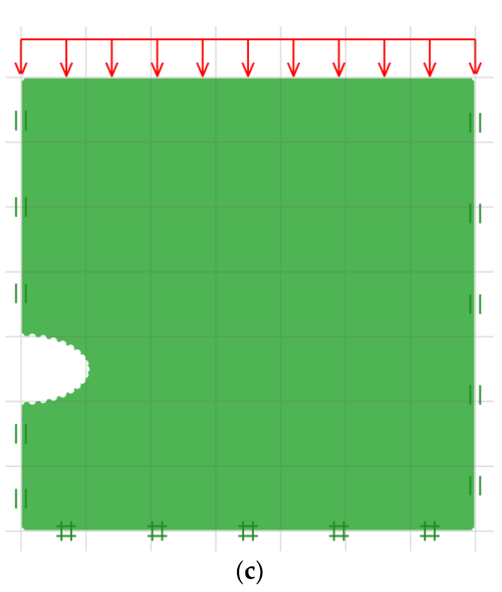
2. Problem Definition

Figure 1 shows the problem geometry of an elliptical tunnel subjected to uniform surcharge loading at the ground surface. The geometry of the elliptical tunnel includes depth (D), a cover (C), and width (B). It should be noted that the standard equation of an ellipse with center (0,0) and a major axis parallel to the x-axis can be expressed as:

$$\frac{x^2}{a^2}+\frac{y^2}{b^2}=1$$

(1)

where B = 2a and D = 2b. In this study, the width–depth ratios of B/D = 0.5, 0.75, 1, 1.333, and 2 are considered. The drained soil is set to be a perfectly plastic Mohr–Coulomb material, and it has an effective cohesion (c’), effective friction angle (ϕ), and unit weight (γ). A vertical uniform pressure (σ_s) is applied overall to the area of the ground surface. Note that the soil unit weight and the surface surcharge generally act as a vertical driving force, resulting in a tunnel collapse.

Six input dimensional parameters (i.e., C, D, B, γ, c′, and ϕ) are considered to have significant impacts on the collapse surcharge at the ground surface σ_s, which is the output dimensional parameter. To reduce the considered parameters in the simulations, the dimensionless technique by Butterfield [41] is employed to convert these six input dimensional parameters to become four dimensionless input parameters by normalising them. As a result, the new relationship between the output dimensionless parameter and the four dimensionless input parameters for the problem of an elliptical tunnel in sands can be written as:

$$\frac{{\sigma }_s}{c^{\prime }}=f(\frac{\gamma D}{c^{\prime }},\frac{C}{D},\frac{B}{D},{\varphi }^{\prime })$$

(2)

where σ_s/c′ denotes the stability factor; γD/c′ denotes the overburden factor; C/D denotes the cover–depth ratio; B/D denotes the width–depth ratio; and ϕ denotes the soil friction angle. Note that the selected normalised form of the stability factor σ_s/c′ is similar to that used in the previous works of the similar problems, e.g., [19,20] (i.e., tunnel stability in cohesive-frictional soils) which will be later used in the verification part of this study.

The selected values of all dimensionless input parameters in this study are shown in

Table 1. Input parameters.

Input Parameters	Values	Average
C/D	1, 2, 3, 4	2.5
B/D	0.5, 0.75, 1, 1.33, 2	1.116
γD/c′	0, 1, 2	1.5
ϕ	0, 5, 10, 15, 20, 25	12.5

. These input and output dimensionless parameters are the main variables in this study that create a nonlinear input–output mapping of the problem of stability of elliptical tunnels, by utilising an ANN model trained by an extreme learning algorithm.

3. Numerical Analysis

In this study, FELA was employed to perform numerical results of the stability of elliptical tunnels. The results from FELA will be used as a training data in the ANN model in the next section. FELA is a widely used numerical method for successfully computing safety factors or limit loads of several problems in the geotechnical engineering field [42,43,44,45,46,47,48,49,50,51]. Commercial FELA software, namely OptumG2 [52], was carried out to derive the stability solutions for tunnel problems in this study. Figure 2a–c presents three typical models generated by OptumG2 for a depth ratio C/D = 4 and different values of B/D = 0.5, 1, and 2, respectively. Only one-half of the domain of the elliptical tunnels was considered in the simulation due to the symmetry of the problem, where the symmetry plane is located at the left of the domain of all three models with B/D = 0.5, 1, and 2 as shown in Figure 2.

Next, the boundaries of this plane strain tunnel problem were fully described. At the left (the symmetry plane) and right boundaries of the domain, the roller supports were set by allowing vertical movements. Additionally, the fixed supports were set along the plane of the bottom boundary, where all vertical and horizontal movements were not permitted to take place. Inside the elliptical tunnel and at the top ground surface, free movements were allowed, indicating the free surfaces at those areas. Note that a uniform surcharge (σ_s) is also applied vertically over the top ground surface. This uniform surcharge at the collapse of the tunnels was optimised by using the loading multiplier technique in OptumG2 based on UB and LB FELA.

The details of the FELA are described next. The soils were discretised into a number of triangular elements distributed over the domain of the tunnel problems in both LB and UB FELA. The collapse surcharge was maximized in the LB analysis by using the loading multiplier technique, satisfying all equilibrium conditions based on the LB FELA scheme that are constructed within the entire domain of the problem. The collapse surcharge was minimised in the UB analysis by also using the loading multiplier technique, where the rate of total work was completed by the external pressure with the total internal power dissipation. In all simulations of the LB and UB FELA models, the domain sizes of all models were carefully selected to be large enough, since the plastic shear zone should be contained within the domain in order to avoid insufficient size effect errors. Thus, the sizes of the right and bottom boundaries were set to be 7D and 2D, respectively, which are sufficient to avoid the effect from insufficient boundaries (see Figure 2).

The powerful feature of mesh adaptivity in OptumG2 was activated in all simulations in order to produce more accurate bound solutions. The number of elements was set to be increased from 5000 (at the first step) to 10,000 elements (at the final step) through five iterations of adaptive meshing. More information regarding this mesh adaptivity feature can be found in the work by Ciria et al. [53]. Examples of typical adaptive meshes of unlined elliptical tunnels in cohesive-frictional soil are demonstrated in Figure 3a–c for the different values of B/D = 0.5, 1, and 2, respectively.

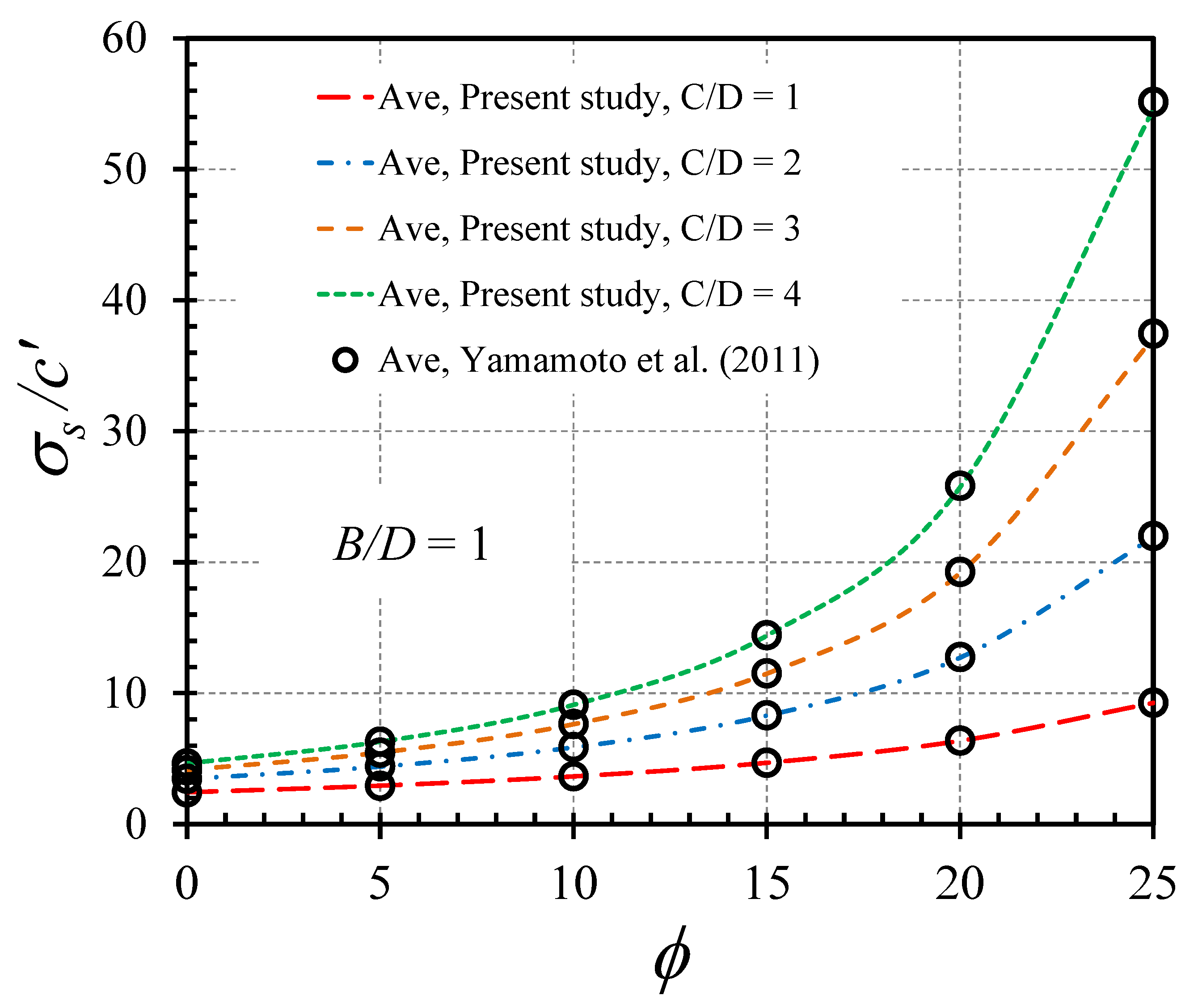
4. FELA Results and Discussion

All numerical results are the average (Ave) results obtained from the average values of the UB and LB FELA solutions, where, in all solutions, the differences between the UB and LB solutions are within 1%. To verify the current solutions, the comparison of the stability factors σ_s/c′ between the present study and a previous work by Yamamoto et al. [19] is shown in Figure 4. Note that the solutions by Yamamoto et al. [19] are limited to the cases of circular tunnels with B/D = 1. In Figure 4, the value of soil unit weight was to be zero so that the dimensionless overburden factor γD/c′ = 0. Thus, the current results are in very good agreement with the Avg solutions by Yamamoto et al. [19], confirming that the computed Ave solutions are very accurate.

All numerical Ave solutions of the elliptical tunnel stability are expressed in

Table 2. Stability factors σ_s /c′ for elliptical tunnels.

γD/c′	B/D	ϕ	C/D = 1	C/D = 2	C/D = 3	C/D = 4
0	0.5	0	3.194	4.042	4.6415	5.112
		5	3.941	5.2585	6.2735	7.11
		10	5.0205	7.197	9.0535	10.671
		15	6.7035	10.6005	14.3025	17.758
		20	9.537	17.311	25.606	34.1285
		25	14.846	32.5035	54.5715	80.1625
	0.75	0	2.8235	3.766	4.3965	4.877
		5	3.449	4.8515	5.8745	6.698
		10	4.3435	6.5475	8.3315	9.8635
		15	5.6975	9.4395	12.83	15.989
		20	7.9025	14.885	22.1915	29.491
		25	11.9115	26.743	45.0285	65.952
	1	0	2.4365	3.4595	4.131	4.6315
		5	2.9435	4.406	5.4625	6.29
		10	3.65	5.875	7.622	9.1015
		15	4.6915	8.2945	11.4835	14.387
		20	6.3665	12.72	19.1735	25.7245
		25	9.2615	21.9155	37.1275	54.594
	1.33	0	1.9845	3.0405	3.7625	4.297
		5	2.346	3.827	4.9115	5.7565
		10	2.844	5.006	6.7365	8.174
		15	3.559	6.8775	9.8775	12.558
		20	4.6385	10.23	15.913	21.5575
		25	6.4805	16.798	29.2085	43.145
	2	0	1.369	2.3015	3.0505	3.637
		5	1.5485	2.8055	3.878	4.7595
		10	1.7905	3.533	5.148	6.533
		15	2.5705	4.6475	7.226	9.6325
		20	2.1125	6.473	10.9655	15.5125
		25	3.293	9.714	18.507	28.4055
1	0.5	0	1.846	1.6285	1.206	0.6655
		5	2.501	2.6405	2.508	2.202
		10	3.451	4.2855	4.785	5.032
		15	4.9415	7.2425	9.2465	10.9705
		20	7.482	13.205	19.229	25.3425
		25	12.383	27.1315	45.591	67.3385
	0.75	0	1.5695	1.4205	1.011	0.471
		5	2.1085	2.3035	2.163	1.8355
		10	2.877	3.7025	4.126	4.287
		15	4.0515	6.1475	7.8615	9.28
		20	6.004	10.8555	15.9195	20.9795
		25	9.5875	21.4915	36.3595	53.6445
	1	0	1.2515	1.1815	0.8005	0.2685
		5	1.6745	1.9235	1.8025	1.4675
		10	2.266	3.098	3.4675	3.562
		15	3.15	5.0775	6.55	7.7195
		20	4.574	8.803	12.9935	17.166
		25	7.0895	16.763	28.6415	42.36
	1.33	0	0.85	0.832	0.5025	−0.003
		5	1.1365	1.413	1.3145	0.9875
		10	1.5315	2.2985	2.6275	2.6665
		15	2.1005	3.7575	4.979	5.903
		20	2.9985	6.3965	9.72	12.9735
		25	4.4975	11.7655	20.696	30.9425
	2	0	0.2685	0.1605	−0.1195	−0.5595
		5	0.397	0.4785	0.37	0.065
		10	0.562	0.9475	1.134	1.0765
		15	0.793	1.682	2.431	2.947
		20	1.117	2.9245	4.892	6.805
		25	1.6395	5.223	10.1485	15.953
2	0.5	0	0.43	−0.834	−2.277	−3.8305
		5	1.016	−0.0105	−1.304	−2.778
		10	1.8475	1.3195	0.4135	−0.811
		15	3.1475	3.777	3.9625	3.726
		20	5.3945	8.93	12.4105	15.7345
		25	9.826	21.3065	35.934	53.1345
	0.75	0	0.244	−0.99	−2.4375	−3.9995
		5	0.727	−0.28	−1.589	−3.0845
		10	1.388	0.8205	−0.171	−1.476
		15	2.39	2.7845	2.6755	2.145
		20	4.066	6.749	9.256	11.528
		25	7.2225	15.9395	26.8835	39.7155
	1	0	0.0105	−1.1685	−2.605	−4.1705
		5	0.3795	−0.5795	−1.89	−3.4055
		10	0.866	0.2925	−0.7695	−2.1495
		15	1.583	1.792	1.413	0.607
		20	2.7585	4.7355	6.351	7.706
		25	4.8905	11.302	19.2535	28.498
	1.33	0	−0.3225	−1.4325	−2.8375	−4.395
		5	−0.0875	−1.02	−2.308	−3.8255
		10	0.2075	−0.431	−1.5525	−3.017
		15	0.645	0.5505	−0.1295	−1.268
		20	1.327	2.413	3.06	3.3055
		25	2.5005	6.4225	11.193	16.616
	2	0	−0.845	−2.001	−3.329	−4.831
		5	−0.766	−1.855	−3.1525	−4.6615
		10	−0.668	−1.657	−2.9515	−4.5875
		15	−0.5315	−1.344	−2.6155	−3.644
		20	−0.3435	−0.7905	−1.8125	−2.648
		25	−0.0305	0.3445	0.49	0.2425

. The results in Table 2 will be used as training data in the ANN approach later in the next section. In this section, some of the results are carried out to investigate the effects of all dimensionless parameters on the stability factor hereafter. First, the effect of the soil friction angle ϕ on σ_s/c′ is shown in Figure 5a,b for the tunnels γD/c′ = 0 and C/D = 2 and 3, respectively. A highly non-linear relationship between ϕ on σ_s/c′ can be observed, where an increase in the friction of soil results in an increasing strength of tunnels. Figure 6a,b presents the relationship between the dimensionless overburden factor γD/c′ and σ_s/c′, where the others are ϕ = 25° and C/D = 1 and 3, respectively. The value of σ_s/c′ gradually decreases as the value of γD/c′ increases. The impact of C/D on σ_s/c′ is shown in Figure 7a,b for (ϕ = 15° and 25° and γD/c′ = 1). It was found from Figure 7 that the relation between C/D and σ_s/c′ is non-linear, where concave curves can be seen in Figure 7a for the case of a small frictional angle. In contrast, convex curves were found in Figure 7b when the values of ϕ were high. Finally, a nonlinear variation of σ_s/c′ and B/D can be noticed in Figure 8a,b for the cases of ϕ = 25° and γD/c′ = 0 and 1, respectively. The plots are for four different values of C/D = 1, 2, 3, and 4. It was found that a nonlinear decrease in the stability factor with the increasing B/D appears in Figure 8. This is in line with the common engineering judgment that a larger B/D ratio causes a lower value of σ_s/c′.

The effects of C/D and B/D on the predicted collapse mechanisms are demonstrated in Figure 9, Figure 10 and Figure 11 for the cases of B/D = 0.5, 1, and 2, respectively. The presented collapse mechanisms correspond to absolute velocity contours of unlined elliptical tunnels in cohesive-frictional soil. In Figure 9, Figure 10 and Figure 11, the sub-figure shows the different cases of C/D = 1, 2, and 4, where other parameters remain the same as γD/c′ = 0 and ϕ = 25°. It can clearly be seen that the failure extent increased with an increased cover-depth ratio (C/D) for all width-depth ratios (B/D). The failure patterns in all figures are like a chimney-type opening of failure. It was also found that the failure extent initially increases when the shape transformed from elliptical to circular (B/D = 0.5 to 1.0). However, failure extent was reduced when a transformation is from circular to elliptical (B/D = 1 to 2).

5. Proposed Models

5.1. Multiple Linear Regression (MLP)

Linear regression is a method of modelling the linear relationship between scalar responses (output known as dependent variables) and explanatory variables (input known as independent variables). Simple linear regression is called such when there is only one independent variable in the relationship. In this study, four independent variables are considered; therefore, the process is called “multiple linear regression”, which is one of the most well-known and straightforward methods in regression problems. Notably, this method can be used as a baseline performance of the machine learning model.

As indicated in Equation (3), the output is a dependent variable that may be determined from the combination of the input or independent variables.

$$y_i={\beta }_0+{\beta }_1{x}_{i1}+{\beta }_2{x}_{i2}+\dots +{\beta }_p{x}_{ip}+ϵ$$

(3)

where $y_i$ = dependent variable (output); $x_{i1}, x_{i1}, \dots x_{ip}$ = independent variables (input); ${\beta }_0$ = y-intercept (constant term); ${\beta }_1, {\beta }_1,\dots , {\beta }_p$ = slope coefficients for each explanatory variable; and $ϵ$ = the model’s error term (also known as the residuals).

A regression model posits that the dependent variable y has a linear relationship with the p-vector of regressors x. An error variable or residual term is an unobserved random variable that represents the noise in the relationship. This paper uses a function of LinearRegression in WEKA to perform the standard least-squares multiple linear regression and optionally attribute selection.

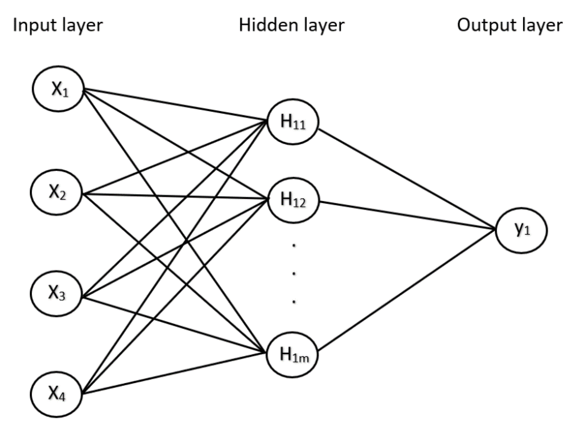
5.2. Artificial Neural Network (ANN)

In this study, an artificial neural network (ANN) was also used. This technique is a data prediction framework based on existing attributes derived from the structure of the human mind. It models the neurological system of the human brain’s processing method for complicated information. A neural network is a computer model made up of a large number of nodes (or neurons) that are linked together. As illustrated in Figure 12, an ANN model is made up of three layers: the input layer, the hidden layer, and the output layer. The first layer is the input layer, through which the feature vector is transferred. In this paper, the input layer is made up of four nodes that indicate C/D, B/D, γD/c′, and ϕ. The hidden layer, which contains a number of neurons, is the second layer. In general, the number of hidden layers and hidden neurons is determined by trial and error (by increasing the number of hidden neurons) until the optimal number is found. This layer’s goal is to convert the data into content that the output layer may use to forecast the data. The last layer is the output layer, which displays a predicted value. In this study, the output layer is made up of a node that presents a predicted stability factor of shallow elliptical tunnels in cohesive-frictional soils. In this case, the network will train through for the specified number of epochs, which is set to be 500.

5.3. Cross-Validation

The partitioning approach into training and testing datasets is unreliable when there are a restricted number of datasets. A more general strategy for offsetting any bias introduced by the specific sample used for holdout is to repeat the entire operation, training and testing, numerous times, using randomly generated samples. The typical method for the model validation of a machine learning methodology is stratified 10-fold cross-validation. This method randomly divides the datasets into ten sections, with the class represented in about the same proportions as in the entire dataset. Before assessing the error rate on the holdout set, each section is performed in turn, and the remaining nine-tenths are later tested. As a result, the learning operation is repeated ten times on different training sets. Finally, the average of the ten errors is computed to produce an overall error estimation. A single tenfold cross-validation, on the other hand, may not be sufficient to get a credible error estimate. Because of the influence of random datasets, separate tenfold cross-validation tests with the same learning system and datasets frequently give different results. Therefore, it is highly advised that the cross-validation process be repeated 10 times, that is, tenfold cross-validation, and the results be averaged. This entails running 100 times on training sets that are each one-tenth the size of the original.

5.4. Performance Measures

Three analysis measures were used in this work to examine the performance of the trained models: correlation coefficient (R), root mean squared error (RMSE), and mean absolute error (MAE).

The correlation coefficient measures the statistical correlation between the expected and actual values. The correlation coefficient varies from 0 for irrelevant results to 1 for fully correlated results. A value smaller than zero, on the other hand, denotes a negative association. Correlation differs from the other metrics in that it is scale-independent, which means that if a certain set of predictions is used, the error remains unchanged if all of the forecasts are multiplied by a fixed factor, while the actual values remain the same. The correlation coefficient can be calculated using Equation (4). Note that a high accuracy model leads to a high correlation coefficient value, whereas the other approaches (e.g., MAE, RMSE, etc.) calculate error instead of accuracy, so that good performance is indicated by lower values.

$$R=\frac{S_{PA}}{\sqrt{S_P{S}_A}}$$

(4)

where $S_{PA}=\frac{{{\displaystyle \sum }}_i\left(p_i-\overline{p}\right)\left(a_i-\overline{a}\right)}{n-1}$; $S_P=\frac{{{\displaystyle \sum }}_i{\left(p_i-\overline{p}\right)}^2}{n-1}$; $S_A=\frac{{{\displaystyle \sum }}_i{\left(a_i-\overline{a}\right)}^2}{n-1};$ $\overline{p}$ and $\overline{a}$ are the average values of p and a variables, respectively; and n is the number of datasets.

The determination coefficient (R-squared, R²) is the square of the correlation coefficient. It is vital to note that, in the case of multiple variables, R² can better quantify the strength of the developed model, since R cannot explain the strength when the number of variables is more than 1 or multiple linear regression is considered. Therefore, R² is used in this study as one of the indicators to measure the performance of the developed model.

Additionally, the mean absolute error (MAE) is a measure of an average of the magnitude of individual errors without taking into consideration their sign. Note that MAE does not exaggerate the influence of outliers—instances in which the prediction error is greater than the others. This is the benefit of using MAE over MSE. Equation (5) depicts the equation for MAE.

$$MAE=\frac{\left|p_1-a_1\right|+\dots +\left|p_n-a_n\right|}{n}$$

(5)

Furthermore, mean-squared error (MSE) is the principal and one of the most commonly used measures. Nevertheless, it should be noted that the square root (root mean squared error, RMSE) is occasionally employed and chosen over MSE. This is because it provides similar dimensions as the predicted value. The mean-squared error is used in many mathematical approaches, because it is the easiest measure to alter mathematically: it is “well-behaved”, as mathematicians say. As mentioned, MSE has similar units as the dependent variable; RMSE is more often used than MSE to compare the performance of the regression model to other random models. It should be noted that a lower MSE and RMSE values suggests a more accurate model.

$$RMSE=\sqrt{\frac{{\left(p_1-a_1\right)}^2+\dots +{\left(p_n-a_n\right)}^2}{n}}$$

(6)

5.5. Multiple Linear Regression (MLR) Equation

First, the regression coefficients of each explanatory variable were optimised by minimising the error in WEKA software. Equation (7) depicts the predictive equation of the stability factor based on multiple linear regression.

$$y=-6.0785x_1-0.8065x_2-4.3909x_3-2.801x_4+1.4307$$

(7)

where y represents the stability factor σ_s/c′, whereas $x_1,x_2,x_3, \mathrm{and} x_4$ are the dimensionless input parameters, namely B/D, ϕ, γD/σ_ci, and C/D, respectively.

It was found that the performance of the developed multiple linear regression equation can be accessed via the statistical tests R², MAE, and RMSE, which are 0.7536, 5.1777, and 7.7086, respectively (see

Table 3. Performance measures of each methodology.

Methodology	R2	Mean Absolute Error (MAE)	Root Mean Squared Error (RMSE)
Multiple Linear Regression (MLR)	0.7536	5.1777	7.7086
Artificial Neural Network (ANN)	0.9967	0.6774	0.9666

).

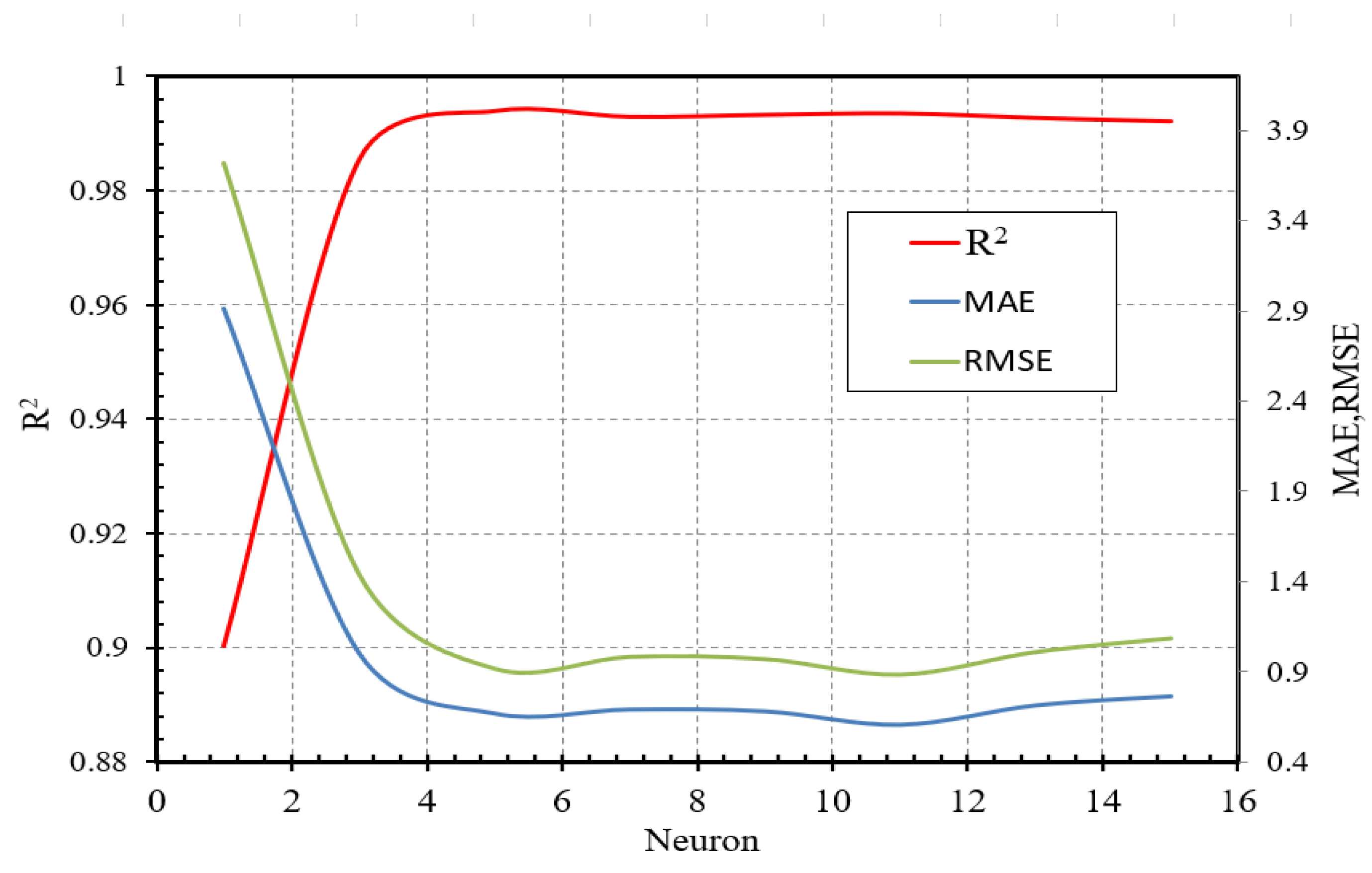
5.6. Details of Proposed Artificial Neural Network (ANN) Model

To improve the performance in terms of the prediction accuracy of ANN models, the number of hidden layers and neurons should be optimised. In the case of stability factor prediction, it was found that only one hidden layer is used sufficiently, with the number of hidden neurons varying. Figure 13 depicts the performance of the models in relation to the number of hidden neurons. It was discovered that increasing the number of neurons until a specific level significantly improves the performance of the ANN model. It can be shown that after a specific level is reached, the performance of the ANN models is likely to stabilise. In this study, the ANN with the architecture of 4-9-1 was chosen as the best ANN model, since it had the lowest MAE and RMSE values and the greatest R² among the models. Figure 14 compares the results generated by the FELA and ANN, which are shown to be quite close. Table 3 also compares the MLR and ANN models’ performance. It is evident that the ANN model outperformed the ANN model. This ideal ANN model with the architecture of 4-9-1 is expected to be employed in future research.

After determining the best ANN architecture design, the approximation general functions may be used to generate outputs by taking into account the weighted inputs and the transfer function. In multiple-layer networks, the layer number defines the superscript on the weight matrix, as shown in Figure 15. In the two-layer tansig/purelin network, the proper notation was utilised. This network may be used to approximate generic functions. It can arbitrarily approximate any function with a finite number of discontinuities given a sufficient number of neurons in the hidden layer. The final weights of each parameter were determined in this section to investigate the influence of each parameter on the stability factor. Figure 15 depicts the dimensions of input, weight, bias, and the output matrices of the optimal ANN model for predicting the stability factor of shallow elliptical tunnels in cohesive-frictional soils. Hence, the predictive Equation (8) can be developed based on the matrices derived from the ANN model in WEKA software.

$$Predicted value=\left[{\displaystyle \sum }_{i=1}^{N}IW{2}_{i}tansig({{\displaystyle \sum }}_{j=1}^{J}IW{1}_{ij}{x}_j+b_{1i})+b_2\right]$$

(8)

where X is the input variables; IW1 and IW2 are the weight matrix in the hidden and output layers, respectively; J is the number of input variables; N is the number of hidden neurons; and b_1i and b₂ are the biases in the hidden and output layers, respectively.

The hidden weight (IW1) was calculated based on the number of input variables (J) and hidden neurons (N) in the hidden layer. As seen in Figure 15, in the output weight matrix (IW2), the number of rows corresponds to the number of hidden layer neurons (N), and the number of columns corresponds to the number of output layer neurons (k). Each neuron in the output layer has its own column. In this scenario, there is just one column in the output layer.

Table 4. Neural network constants of the optimal model for stability prediction of shallow elliptical tunnels in cohesive-frictional soils.

Hidden Layer Neurons (i)		Hidden Layer Bias (b1)		Hidden Weight IW1
				B/D (j = 1)	ϕ (j = 2)		γD/σci (j = 3)		C/D (j = 4)
1		−1.8972		0.4966	0.3791		−0.4916		0.2817
2		−1.4926		0.5715	−0.2262		0.1143		0.7693
3		−5.1539		1.0019	−1.0584		0.2803		2.9550
4		−0.5608		−0.0674	0.1779		0.0326		0.3379
5		−0.8563		1.1308	−0.3793		−0.0940		0.8034
6		−0.6919		0.0469	−0.0108		−0.0048		0.3094
7		−3.2286		0.5069	−0.1487		−0.4482		1.5636
8		−1.4544		−0.7200	1.1056		0.4755		0.8460
9		−1.9549		1.6058	−0.0265		0.9068		−0.1308
Output layer node (k)	Output layer bias (b2)	Output weight IW2
		i = 1	i = 2	i = 3	i = 4	i = 5	i = 6	i = 7	i =8	i = 9
1	2.6100	−0.8506	−0.7820	−3.5971	−0.0863	−0.8197	−0.0514	−1.6245	0.6988	1.8593

shows the neural network constants of the best ANN model, including the weight matrix and bias. These constants can be used to evaluate the stability factor calculation of shallow elliptical tunnels in cohesive-frictional soils. These ideal ANN network values may be utilised to create prediction equation functions and test them on fresh datasets with varied parameter changes within specified ranges.

6. Conclusions

The study established a machine learning-aided prediction of the stability of shallow elliptical tunnels in cohesive-frictional soils. Four input dimensionless parameters included the dimensionless overburden factor γD/c′, the cover–depth ratio C/D, the width–depth ratio B/D, and the soil friction angle ϕ. The influences of all input dimensionless parameters on the solutions of the stability factor σ_s/c′ were investigated. The solutions were computed using finite element limit analysis (FELA). An artificial neural network (ANN) model was then developed based on the training data of the FELA solutions. Since the computational time to develop the algorithm of FELA is high and the use of the FELA software for practicing engineers to obtain the stability solutions of elliptical tunnels in sands varies case by case, the proposed schemes of the ANN model were developed in this study. In addition, a commercial software is not always user friendly, necessitating the employment of extra resources capable of giving information beneficial for decision making. Therefore, the proposed solutions are not only for practicing engineers, but also for designers who can potentially use the developed predictive equations to conveniently calculate the stability of the tunnel. This will help them to understand the capacity and stability of the tunnel and whether it can withstand the actual surcharge load on the ground surface without loss of stability or not. The following conclusions can be drawn in this study.

• The combination of FELA solutions and the ANN is presented as a guide for geotechnical engineers. Note that the proposed predictive model for the stability factor of this problem can be evaluated based on the complex solutions that are derived from the matrices obtained in this study.
• It is notable that just one hidden layer with seven neurons can sufficiently build a reliable high-performance neural network model.
• The proposed model can be used to accurately predict the stability factor of shallow elliptical tunnels in cohesive-frictional soils based on a new dataset using the weight and bias matrices derived in this study.
• The limitation of the proposed model is that the new dataset should be within the ranges provided in this study.

References

1. Sloan, S.; Assadi, A. Undrained stability of a plane strain heading. Can. Geotech. J. 1994, 31, 443–450. [Google Scholar] [CrossRef]
2. Ukritchon, B.; Keawsawasvong, S.; Yingchaloenkitkhajorn, K. Undrained face stability of tunnels in Bangkok subsoils. Int. J. Geotech. Eng. 2016, 11, 262–277. [Google Scholar] [CrossRef]
3. Mair, R.J. Centrifugal Modelling of Tunnel Construction in Soft Clay. Ph.D. Thesis, Cambridge University, Cambridge, UK, 1979. [Google Scholar] [CrossRef]
4. Shiau, J.; Al-Asadi, F. Three-Dimensional Analysis of Circular Tunnel Headings Using Broms and Bennermark’s Original Stability Number. Int. J. Géoméch. 2020, 20, 06020015. [Google Scholar] [CrossRef]
5. Ukritchon, B.; Keawsawasvong, S. Lower bound stability analysis of plane strain headings in Hoek-Brown rock masses. Tunn. Undergr. Space Technol. 2018, 84, 99–112. [Google Scholar] [CrossRef]
6. Ukritchon, B.; Keawsawasvong, S. Stability of Retained Soils Behind Underground Walls with an Opening Using Lower Bound Limit Analysis and Second-Order Cone Programming. Geotech. Geol. Eng. 2018, 37, 1609–1625. [Google Scholar] [CrossRef]
7. Ukritchon, B.; Keawsawasvong, S. Design equations for undrained stability of opening in underground walls. Tunn. Undergr. Space Technol. 2017, 70, 214–220. [Google Scholar] [CrossRef]
8. Fraldi, M.; Guarracino, F. Limit analysis of collapse mechanisms in cavities and tunnels according to the Hoek–Brown failure criterion. Int. J. Rock Mech. Min. Sci. 2009, 46, 665–673. [Google Scholar] [CrossRef]
9. Davis, E.H.; Gunn, M.J.; Mair, R.J.; Seneviratine, H.N. The stability of shallow tunnels and underground openings in cohesive material. Geotechnique 1980, 30, 397–416. [Google Scholar] [CrossRef]
10. Ukritchon, B.; Keawsawasvong, S. Lower bound solutions for undrained face stability of plane strain tunnel headings in anisotropic and non-homogeneous clays. Comput. Geotech. 2019, 112, 204–217. [Google Scholar] [CrossRef]
11. Ukritchon, B.; Yingchaloenkitkhajorn, K.; Keawsawasvong, S. Three-dimensional undrained tunnel face stability in clay with a linearly increasing shear strength with depth. Comput. Geotech. 2017, 88, 146–151. [Google Scholar] [CrossRef]
12. Drucker, D.C.; Prager, W.; Greenberg, H.J. Extended limit design theorems for continuous media. Q. Appl. Math. 1952, 9, 381–389. [Google Scholar] [CrossRef] [Green Version]
13. Chen, W.F.; Liu, X.L. Limit Analysis in Soil Mechanics; Elsevier: Amsterdam, The Netherlands, 1990. [Google Scholar]
14. Sloan, S. Geotechnical stability analysis. Géotechnique 2013, 63, 531–571. [Google Scholar] [CrossRef] [Green Version]
15. Sloan, S.W.; Assadi, A. Undrained stability of a square tunnel whose strength increases linearly with depth. Comput. Geotech. 1991, 12, 321–346. [Google Scholar] [CrossRef]
16. Wilson, D.W.; Abbo, A.J.; Sloan, S.W.; Lyamin, A.V. Undrained stability of a circular tunnel where the shear strength increases linearly with depth. Can. Geotech. J. 2011, 48, 1328–1342. [Google Scholar] [CrossRef]
17. Abbo, A.J.; Wilson, D.W.; Sloan, S.; Lyamin, A. Undrained stability of wide rectangular tunnels. Comput. Geotech. 2013, 53, 46–59. [Google Scholar] [CrossRef]
18. Wilson, D.W.; Abbo, A.J.; Sloan, S.W. Undrained stability of tall tunnels. In Proceedings of the 14th International Conference of International Association for Computer Methods and Recent Advances in Geomechanics, Kyoto, Japan, 22–25 September 2014. [Google Scholar]
19. Yamamoto, K.; Lyamin, A.; Wilson, D.W.; Sloan, S.; Abbo, A. Stability of a circular tunnel in cohesive-frictional soil subjected to surcharge loading. Comput. Geotech. 2011, 38, 504–514. [Google Scholar] [CrossRef]
20. Yamamoto, K.; Lyamin, A.; Wilson, D.W.; Sloan, S.; Abbo, A. Stability of a single tunnel in cohesive–frictional soil subjected to surcharge loading. Can. Geotech. J. 2011, 48, 1841–1854. [Google Scholar] [CrossRef]
21. Keawsawasvong, S.; Ukritchon, B. Undrained stability of plane strain active trapdoors in anisotropic and non-homogeneous clays. Tunn. Undergr. Space Technol. 2020, 107, 103628. [Google Scholar] [CrossRef]
22. Keawsawasvong, S.; Ukritchon, B. Design equation for stability of shallow unlined circular tunnels in Hoek-Brown rock masses. Bull. Eng. Geol. Environ. 2020, 79, 4167–4190. [Google Scholar] [CrossRef]
23. Keawsawasvong, S.; Likitlersuang, S. Undrained stability of active trapdoors in two-layered clays. Undergr. Space 2020, 6, 446–454. [Google Scholar] [CrossRef]
24. Keawsawasvong, S.; Shiau, J. Stability of active trapdoors in axisymmetry. Undergr. Space 2021, 7, 50–57. [Google Scholar] [CrossRef]
25. Ukritchon, B.; Keawsawasvong, S. Stability of unlined square tunnels in Hoek-Brown rock masses based on lower bound analysis. Comput. Geotech. 2018, 105, 249–264. [Google Scholar] [CrossRef]
26. Ukritchon, B.; Keawsawasvong, S. Undrained Stability of Unlined Square Tunnels in Clays with Linearly Increasing Anisotropic Shear Strength. Geotech. Geol. Eng. 2019, 38, 897–915. [Google Scholar] [CrossRef]
27. Yang, F.; Zhang, J.; Yang, J.; Zhao, L.; Zheng, X. Stability analysis of unlined elliptical tunnel using finite element upper-bound method with rigid translatory moving elements. Tunn. Undergr. Space Technol. 2015, 50, 13–22. [Google Scholar] [CrossRef]
28. Yang, F.; Sun, X.; Zheng, X.; Yang, J. Stability analysis of a deep buried elliptical tunnel in cohesive–frictional (c–ϕ) soils with a nonassociated flow rule. Can. Geotech. J. 2017, 54, 736–741. [Google Scholar] [CrossRef]
29. Yang, F.; Sun, X.; Zou, J.; Zheng, X. Analysis of an elliptical tunnel affected by surcharge loading. Proc. Inst. Civ. Eng. -Geotech. Eng. 2019, 172, 312–319. [Google Scholar] [CrossRef]
30. Zhang, J.; Yang, J.; Yang, F.; Zhang, X.; Zheng, X. Upper-Bound Solution for Stability Number of Elliptical Tunnel in Cohesionless Soils. Int. J. Géoméch. 2017, 17, 06016011. [Google Scholar] [CrossRef]
31. Dutta, P.; Bhattacharya, P. Determination of internal pressure for the stability of dual elliptical tunnels in soft clay. Géoméch. Geoengin. 2019, 16, 67–79. [Google Scholar] [CrossRef]
32. Amberg, R. Design and construction of the Furka base tunnel. Rock Mech. Rock Eng. 1983, 16, 215–231. [Google Scholar] [CrossRef]
33. Wone, M.; Nasri, V.; Ryzhevskiy, M. Rock tunnelling challenges in Manhattan. In Claiming the Underground Space, 1st ed.; Routledge: Oxfordshire, UK, 2003; Volume 1, pp. 145–151. [Google Scholar]
34. Miura, K. Design and construction of mountain tunnels in Japan. Tunn. Undergr. Space Technol. 2003, 18, 115–126. [Google Scholar] [CrossRef]
35. Miura, K.; Yagi, H.; Shiroma, H.; Takekuni, K. Study on design and construction method for the New Tomei–Meishin expressway tunnels. Tunn. Undergr. Space Technol. 2003, 18, 271–281. [Google Scholar] [CrossRef]
36. Hochmuth, W.; Kritschke, A.; Weber, J. Subway construction in Munich, developments in tunneling with shotcrete support. Rock Mech. Rock Eng. 1987, 20, 1–38. [Google Scholar] [CrossRef]
37. Li, A.; Khoo, S.; Lyamin, A.; Wang, Y. Rock slope stability analyses using extreme learning neural network and terminal steepest descent algorithm. Autom. Constr. 2016, 65, 42–50. [Google Scholar] [CrossRef]
38. Li, A.-J.; Lim, K.; Fatty, A. Stability evaluations of three-layered soil slopes based on extreme learning neural network. Transactions of the Chinese Institute of Engineers, Series A. J. Chin. Inst. Eng. 2020, 43, 628–637. [Google Scholar] [CrossRef]
39. Qian, Z.; Li, A.; Chen, W.; Lyamin, A.; Jiang, J. An artificial neural network approach to inhomogeneous soil slope stability predictions based on limit analysis methods. Soils Found. 2019, 59, 556–569. [Google Scholar] [CrossRef]
40. Keawsawasvong, S.; Seehavong, S.; Ngamkhanong, C. Application of Artificial Neural Networks for Predicting the Stability of Rectangular Tunnels in Hoek–Brown Rock Masses. Front. Built Environ. 2022, 8, 837745. [Google Scholar] [CrossRef]
41. Butterfield, R. Dimensional analysis for geotechnical engineers. Geotechnique 1999, 49, 357–366. [Google Scholar] [CrossRef]
42. Ukritchon, B.; Keawsawasvong, S. Unsafe Error in Conventional Shape Factor for Shallow Circular Foundations in Normally Consolidated Clays. J. Geotech. Geoenviron. Eng. 2017, 143, 02817001. [Google Scholar] [CrossRef]
43. Ukritchon, B.; Keawsawasvong, S. Error in Ito and Matsui’s Limit-Equilibrium Solution of Lateral Force on a Row of Stabilizing Piles. J. Geotech. Geoenviron. Eng. 2017, 143, 02817004. [Google Scholar] [CrossRef]
44. Keawsawasvong, S.; Ukritchon, B. Undrained lateral capacity of I-shaped concrete piles. Songklanakarin J. Sci. Technol. 2017, 39, 751–758. [Google Scholar]
45. Keawsawasvong, S.; Ukritchon, B. Finite element analysis of undrained stability of cantilever flood walls. Int. J. Geotech. Eng. 2016, 11, 355–367. [Google Scholar] [CrossRef]
46. Ukritchon, B.; Wongtoythong, P.; Keawsawasvong, S. New design equation for undrained pullout capacity of suction caissons considering combined effects of caisson aspect ratio, adhesion factor at interface, and linearly increasing strength. Appl. Ocean Res. 2018, 75, 1–14. [Google Scholar] [CrossRef]
47. Ukritchon, B.; Keawsawasvong, S. Design equations of uplift capacity of circular piles in sands. Appl. Ocean Res. 2019, 90, 101844. [Google Scholar] [CrossRef]
48. Ukritchon, B.; Yoang, S.; Keawsawasvong, S. Three-dimensional stability analysis of the collapse pressure on flexible pavements over rectangular trapdoors. Transp. Geotech. 2019, 21, 100277. [Google Scholar] [CrossRef]
49. Ukritchon, B.; Yoang, S.; Keawsawasvong, S. Undrained stability of unsupported rectangular excavations in non-homogeneous clays. Comput. Geotech. 2019, 117, 103281. [Google Scholar] [CrossRef]
50. Ukritchon, B.; Keawsawasvong, S. Undrained lower bound solutions for end bearing capacity of shallow circular piles in non-homogeneous and anisotropic clays. Int. J. Numer. Anal. Methods Geomech. 2020, 44, 596–632. [Google Scholar] [CrossRef]
51. Yodsomjai, W.; Keawsawasvong, S.; Senjuntichai, T. Undrained Stability of Unsupported Conical Slopes in Anisotropic Clays Based on Anisotropic Undrained Shear Failure Criterion. Transp. Infrastruct. Geotechnol. 2021, 8, 557–568. [Google Scholar] [CrossRef]
52. Krabbenhoft, K.; Lyamin, A.; Krabbenhoft, J. Optum Computational Engineering (OptumG2 Version G2 2020_2020.08.17). Available online: www.optumce.com (accessed on 1 July 2020).
53. Ciria, H.; Peraire, J.; Bonet, J. Mesh adaptive computation of upper and lower bounds in limit analysis. Int. J. Numer. Methods Eng. 2008, 75, 899–944. [Google Scholar] [CrossRef]
Figure 1. Problem definition of an unsupported elliptical tunnel in cohesive-frictional soil.
Buildings 12 00444 g001
Figure 2. Model geometry for three unlined elliptical tunnels in cohesive-frictional soil. (a) B/D = 0.5, (b) B/D = 1, (c) B/D = 2.
Buildings 12 00444 g002aBuildings 12 00444 g002b
Figure 3. Typical adaptive meshes of unlined elliptical tunnels in cohesive-frictional soil. (a) B/D = 0.5, (b) B/D = 1, (c) B/D = 2.
Buildings 12 00444 g003
Figure 4. Comparison of the stability factors σs /c′ (γD/c = 0 and B/D = 1) between the present study and Yamamoto et al. [19].
Buildings 12 00444 g004
Figure 5. Influence of ϕ on the stability factors σs/c′ (γD/c′ = 0). (a) C/D = 2, (b) C/D = 3.
Buildings 12 00444 g005
Figure 6. Influence of γD/c on the stability factors σs/c′ (ϕ = 25°). (a) C/D = 1, (b) C/D = 3.
Buildings 12 00444 g006
Figure 7. Influence of C/D on the stability factors σs/c′ (γD/c = 1). (a) ϕ = 15, (b) ϕ = 25.
Buildings 12 00444 g007
Figure 8. Influence of B/D on the stability factors σs/c′ (ϕ = 25°). (a) γD/c′ = 0, (b) γD/c′ = 1.
Buildings 12 00444 g008
Figure 9. Absolute velocity contours of unlined elliptical tunnels in cohesive-frictional soil with B/D = 0.5, γD/c′ = 0, and ϕ = 25°. (a) C/D = 1, (b) C/D = 2, (c) C/D = 4.
Buildings 12 00444 g009
Figure 10. Absolute velocity contours of unlined elliptical tunnels in cohesive-frictional soil with B/D = 1, γD/c′ = 0, and ϕ = 25°. (a) C/D = 1, (b) C/D = 2, (c) C/D = 4.
Buildings 12 00444 g010
Figure 11. Absolute velocity contours of unlined elliptical tunnels in cohesive-frictional soil with B/D = 2, γD/c′ = 0, and ϕ = 25°. (a) C/D = 1, (b) C/D = 2, (c) C/D = 4.
Buildings 12 00444 g011aBuildings 12 00444 g011b
Figure 12. ANN architecture.
Buildings 12 00444 g012
Figure 13. Performance evaluation of elliptical tunnel models against the number of hidden neurons.
Buildings 12 00444 g013
Figure 14. Comparison between FELA solution and that predicted using ANN.
Buildings 12 00444 g014
Figure 15. Multilayer networks with weight matrix.
Buildings 12 00444 g015