Article

Vibration-Based and Near Real-Time Seismic Damage Assessment Adaptive to Building Knowledge Level

1
Department of Civil and Environmental Engineering, University of Strathclyde, Glasgow G1 1XQ, UK
2
School of Civil Engineering, University College Dublin, D04V1W8 Dublin, Ireland
3
European Centre for Training and Research in Earthquake Engineering (EUCENTRE), 27100 Pavia, Italy
4
French Geological Survey (BRGM), 45060 Orléans, France
5
Multidisciplinary Institute for Environmental Studies Ramon Magalef (IMEM), University of Alicante, 03690 Alicante, Spain
6
Department Applied Physics Faculty of Sciences, University of Alicante, 03690 Alicante, Spain
*
Author to whom correspondence should be addressed.
Buildings 2022, 12(4), 416; https://doi.org/10.3390/buildings12040416
Submission received: 22 February 2022 / Revised: 24 March 2022 / Accepted: 26 March 2022 / Published: 30 March 2022
(This article belongs to the Collection Structural Analysis for Earthquake-Resistant Design of Buildings)

Abstract

:
This paper presents a multi-level methodology for near real-time seismic damage assessment of multi-story buildings, tailored to the available level of knowledge and information from sensors. The proposed methodology relates changes in the vibratory characteristics of a building—evaluated via alternative dynamic identification techniques—to the European Macroseismic Scale (EMS-98) damage grades. Three distinct levels of knowledge are considered for the building, with damage classification made through (i) empirical formulation based on quantitative ranges reported in the literature, (ii) analytical formulation exploiting the effective stiffness concept, and (iii) numerical modelling including a simplified equivalent single-degree-of-freedom model or a detailed finite element model of the building. The scope of the study is twofold: to construct a framework for integrating structural health monitoring into seismic damage assessment and to evaluate consistencies/discrepancies among different identification techniques and model-based and model-free approaches. The experimental data from a multi-story building subject to sequential shaking are used to demonstrate the proposed methodology and compare the effectiveness of the different approaches to damage assessment. The results show that accurate damage estimates can be achieved not only using model-driven approaches with enhanced information but also model-free alternatives with scarce information.

1. Introduction

Accurate evaluation of post-earthquake building status in a rapid response setting remains an enduring challenge in structural and earthquake engineering. Traditional techniques for assessing post-event conditions rely on visual inspection to identify the extent of building damage. A conventional visual inspection process relies on soliciting an expert team to perform site visits, view damage patterns observable on the building exposed to a seismic event, collect imagery evidence, and complete the procedure by filling in the designated reconnaissance reports [1]. Rapid identification of potentially damaged buildings is crucial for timely decision making about repair and retrofit [2] and minimizing service disruptions while constrained to a specific budget [3]. As apparent from the state-of-the-art, visual inspections are essential to assessing the building condition following an earthquake. However, they suffer from many limitations: they are dangerous, expensive, time-consuming, and potentially inaccurate. This can have a negative impact on post-earthquake emergency response and recovery. The latest trends in visual inspection lean toward automated processing of damage indicator images with the help of advanced computer vision techniques [4]. However, even in such technology-engaged approaches, there is still a reliance on imagery data collected/assisted with human labour (e.g., [5]), which can pose risks to the operator if a building is damaged. Remote vehicular technologies can assist with visual inspections [6], but the required technology has yet to reach full maturity.
With the advent of sensor, computation, and communication systems as well as developments in sophisticated signal processing and system identification algorithms, structural health monitoring (SHM) has emerged as a promising technology-driven solution for the rapid damage assessment of civil infrastructure. Dating back to the 1980s, modern SHM has found function as a damage assessment technique based on changes in vibration characteristics [7]. Rytter [8] first presented a typical SHM flowchart based on 1-existence, 2-location, 3-extent, and 4-consequence. Given a broad series of successful implementations in the field, the ultimate SHM phase, which addresses consequence, is still the phase that is most open for exploration. Moreover, SHM’s integration with post-earthquake damage assessment is formulated in various ways depending on the weights of data and model-driven perspectives. Model-driven approaches lean towards updating damage-sensitive physical parameters, whereas data-driven approaches use model-free metrics to define damage state.
If essential modelling information is available, sensor-engaged SHM approaches connected to performance-based earthquake engineering (PBEE) schemes can potentially predict accurate earthquake-induced damage states and corresponding losses of instrumented buildings [9]. Several analytical methods have been formulated to relate seismic shaking to structure-specific seismic performance and losses on the basis of available sensor data (e.g., [10,11,12]). However, the structural modelling necessary for a PBEE-driven process requires significant effort, and modelling details may be unavailable, especially for region-scale or system-wide assessments. Therefore, despite methodological advancements in probabilistic mechanics and earthquake engineering, a rapid and scalable assessment technique involving simplified structural modelling and SHM data is still in high demand (e.g., [13,14]). Initiatives such as that of Goulet [15], which connect vibration-based SHM to damage assessment in a model-free setting, can be particularly useful in the absence of data on structural properties. A paradigm shift from model-driven to data-driven approaches is necessary if near real-time computation aims are to be achieved. However, this transition depends on the availability of building knowledge and an ability to convert this information to a mathematical model, and a baseline framework in the absence of such information. In that sense, a collection of different strategies that account for different building knowledge levels should be compared. Besides, there is a need to adopt an adaptive approach to this challenge, reflecting variations in the amount of information available on the SHM-integrated seismic damage assessment solution.
Motivated by these needs in the context of rapid responses to earthquakes and the corresponding research gaps in near real-time damage assessment with instrumentation and vibration-based SHM, this study has been performed within the 2019–2022 European Horizon 2020 project TURNkey (Towards more Earthquake-resilient Urban Societies through a Multi-sensor-based Information System enabling Earthquake Forecasting, Early Warning and Rapid Response actions). One of the key ambitions of the TURNkey project is to follow loss assessment methodologies based on the level of data availability (LoDA), or hereinafter, knowledge levels [16]. Consistent with this aim, this study proposes a vibration-based damage identification methodology that is tailored to the specific knowledge level of the building, requiring minimal expert intervention and facilitating rapid deployments that adapt to the available building information. According to the goals of this paper, changes in dynamic building parameters, evaluated with alternative vibration-based identification tools, can be used for a quantitative, rapid, automated, and sensor-driven evaluation of the building damage state, which can be described in terms of the commonly accepted EMS-98 grades [17].
Three knowledge-level-specific vibration-based approaches are presented to consolidate SHM-integrated damage assessment under various building knowledge levels. Knowledge Level 1 (KL1) only involves information from accelerometric sensor data. KL2 requires enough information to construct the roof displacement-total base shear backbone curve for the building, and finally, KL3 represents a comprehensive knowledge level such that a detailed and accurate numerical model of the building can be created. Compatible with the available knowledge level, empirical, analytical, and numerical damage prediction approaches are proposed that rely on the successful determination of vibration period elongation with an array of identification algorithms. The proposed approaches are verified and compared, considering a large-scale building specimen subject to cumulative damage throughout a series of shaking table tests.
The remainder of the paper is structured as follows: Section 2 introduces a set of alternative techniques employed for identifying the dynamic properties of multi-story buildings, namely the output-only frequency domain decomposition (FDD) and its enhanced realization (E)FDD, and two single-input single-output (SISO) approaches based on the Stockwell transform and Wavelet transform. Afterwards, hierarchical and knowledge-dependent damage classification approaches are introduced, namely the (i) empirical, (ii) analytical, and (iii) numerical approaches. Section 3 introduces the experimental setup of a four-story building structure, which experienced cumulative damage due to a repetitive series of ground motion excitations, and Section 4 provides details of the modelling scheme. Section 5 presents the results of applying the dynamic identification and damage classification techniques. Finally, Section 6 outlines the conclusions drawn from the study.

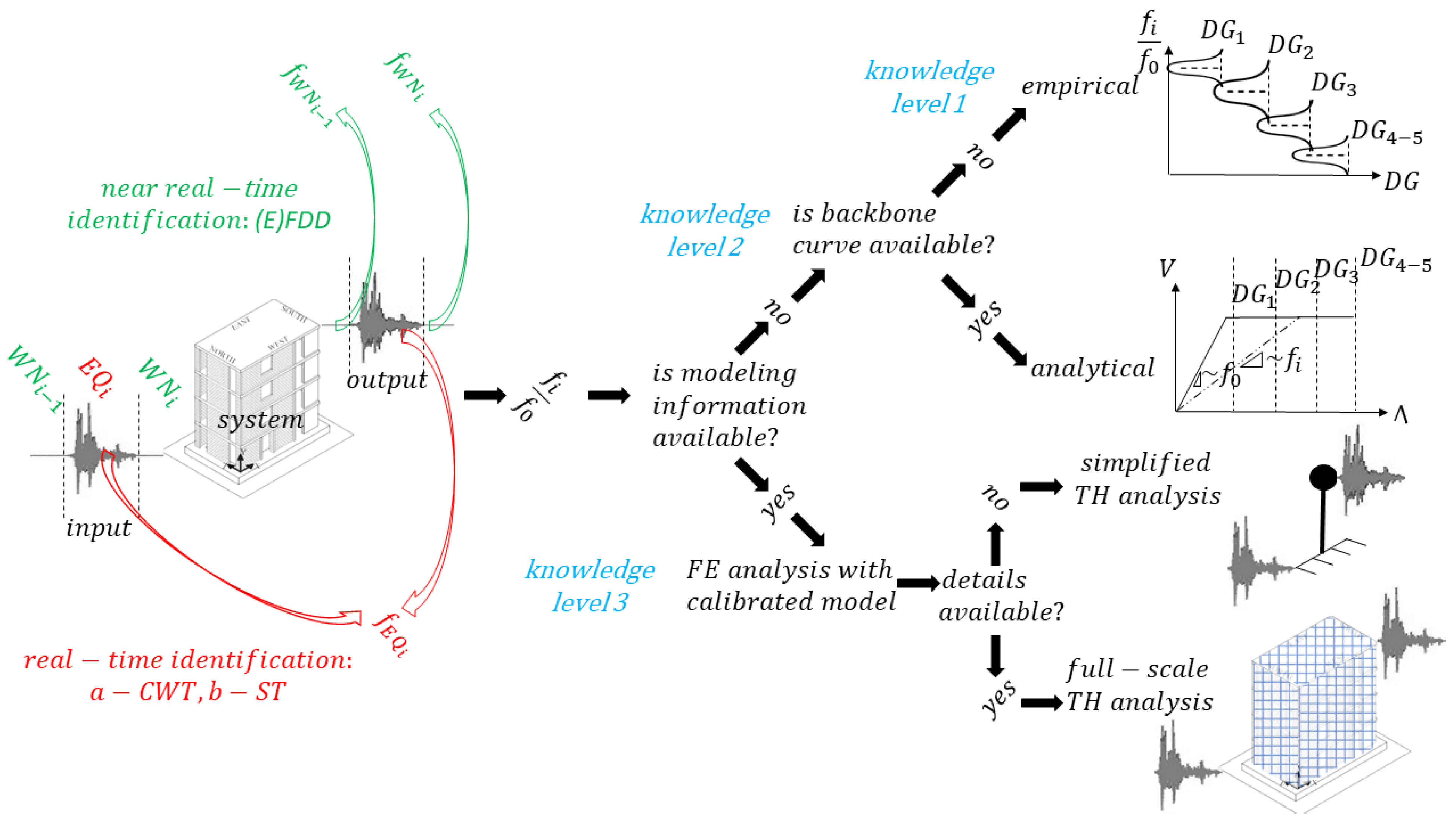
2. Dynamic Identification and Damage Prediction Methods

This section illustrates the main features of the approaches adopted for dynamic identification through SHM and subsequent damage prediction using the results obtained in SHM. For SHM, two noise-based (i.e., (E)FDD and wavelet transformation) and two strong motion-based (i.e., wavelet and Stockwell transformations) approaches are implemented and then applied. Three different approaches are followed for damage prediction depending on knowledge levels. Figure 1 provides an overview of three knowledge levels, three dynamic identification techniques, and three knowledge-level-compatible, hierarchical damage classification approaches. The number of sensors required is limited and can be as low as one accelerometer node for output-only and two accelerometers for SISO cases due to minor input from the SHM system (i.e., period elongation).

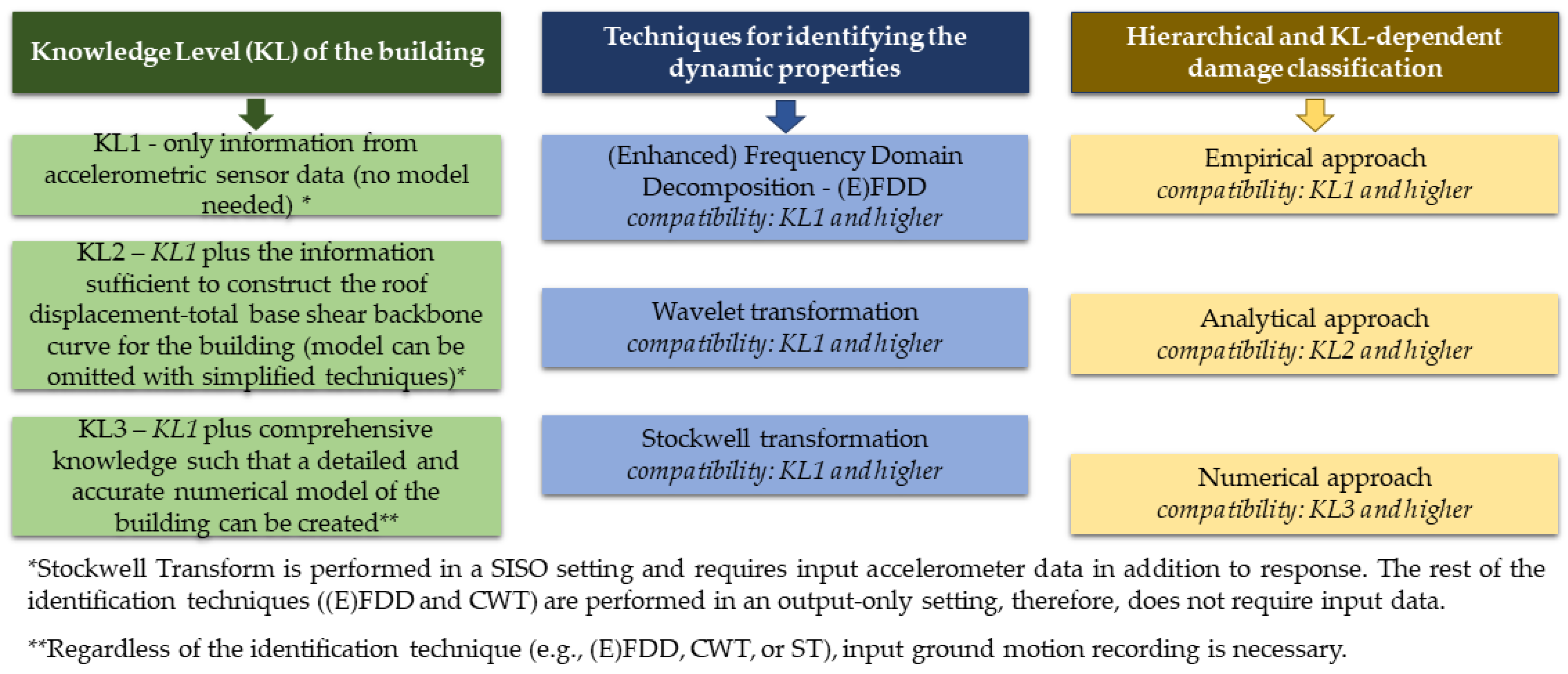
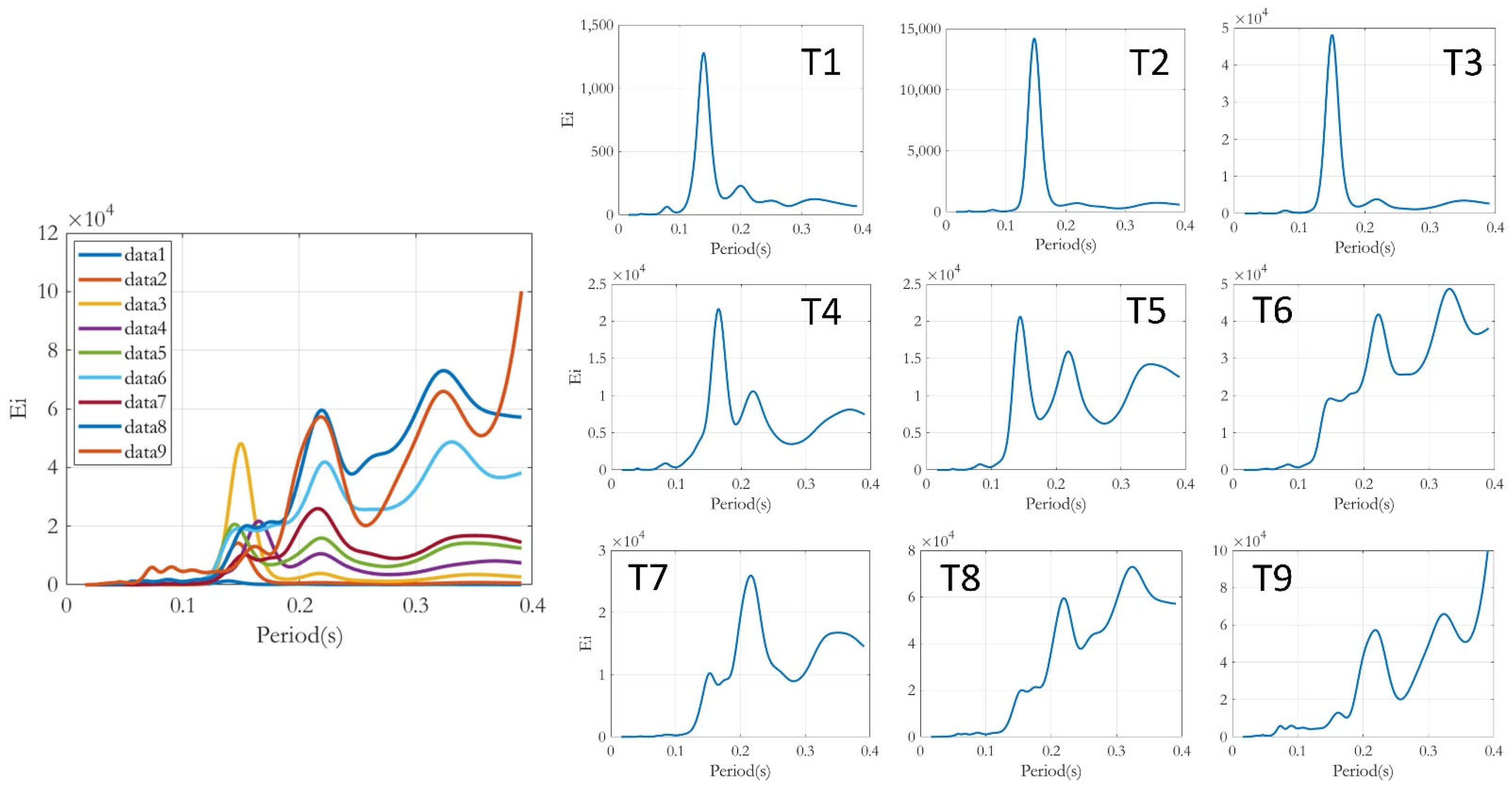
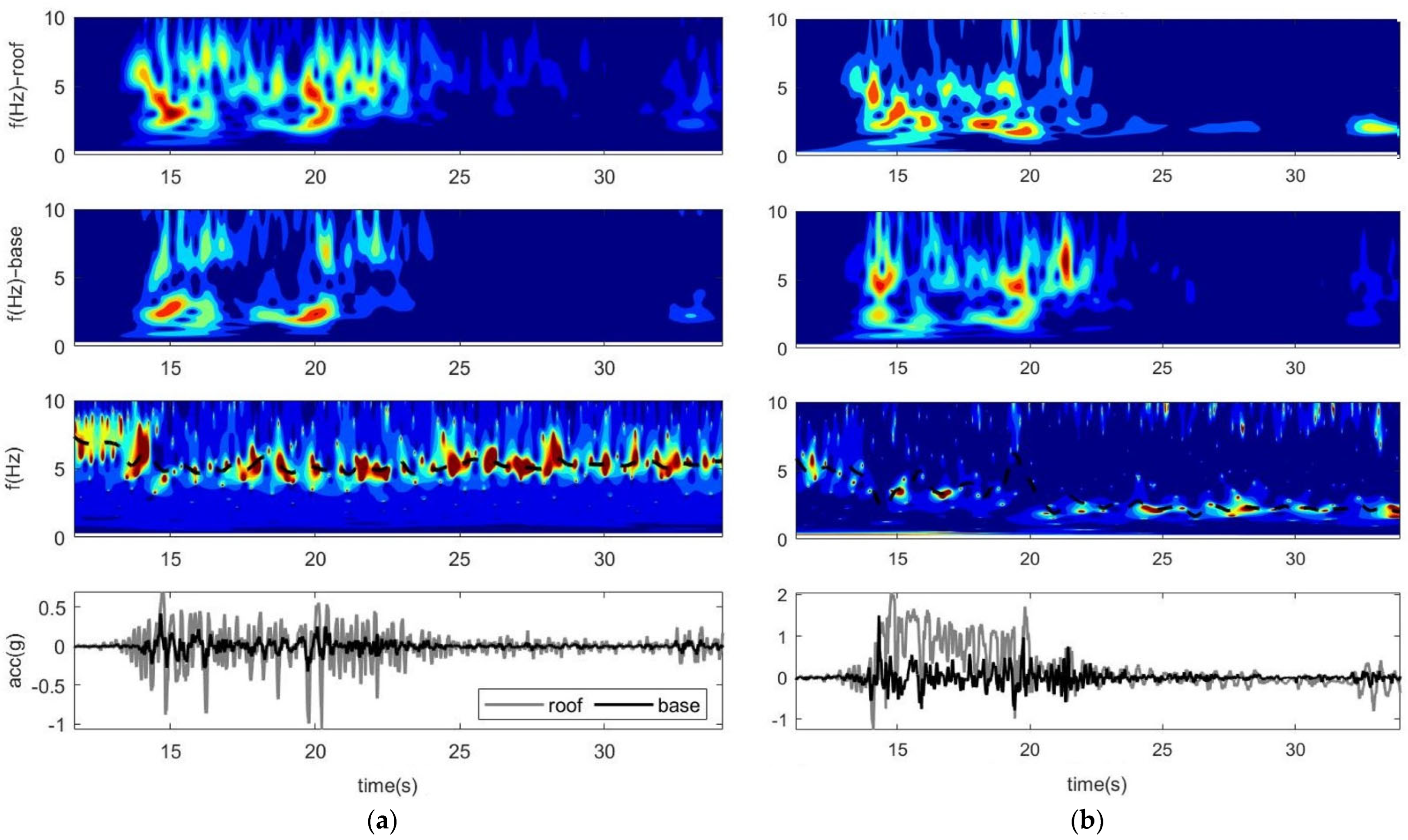
2.1. Overview of Selected Tools for Dynamic Identification

Both Frequency Domain Decomposition (FDD) and its successor Enhanced Frequency Domain Decomposition (E)FDD have been used as vibration-based SHM approaches. Developed by Brincker et al. [18], FDD is an intuitive frequency-domain method suitable for modal identification under operational conditions. FDD is an output-only technique, which assumes the system input is white noise and relies on the synchronous acquisition of multi-channel dynamic response data from the structure of interest to identify modal frequencies and mode shapes. The method uses the Power Spectral Density (PSD) matrix of the multi-channel response as a function of frequency and performs singular value decomposition to obtain the maximum eigenvalues observed on the frequency domain. Eigenvectors provide the mode shapes corresponding to discrete frequencies where the eigenvalues are maximized. Equation (1) expresses the core FDD equation decomposing the PSD matrix into its eigenvalues and eigenvectors, which are efficient in identifying modal frequencies and mode shapes, respectively.
S y y ( w ) = U ( w ) · Σ ( w ) · U H ( w )
where S y y ( w ) is the PSD matrix of the response vector y, U ( w ) is the unitary matrix of the singular vectors, Σ ( w ) is the diagonal matrix of the singular values, and H denotes the complex conjugate transpose operator. In (E)FDD ([19,20]), after carrying out Singular Value Decomposition (SVD), the data are inverted from frequency spectra back into time series to obtain autocorrelation functions representative of the structural dynamics of single degree of freedom systems (into which the original structure may be decomposed). The damping ratios and natural frequencies could be jointly inverted through proper interpolation of the autocorrelation functions. Vibrating modes are also identified, starting from the singular vectors belonging to the neighbourhood of each peak that was previously identified.
In addition to the use of (E)FDD, the Continuous Wavelet Transform (CWT) method is employed to obtain the spectral decomposition more accurately. The basic idea of the CWT method is to determine a function ψ(t) that can generate a basis for the entire domain of function x(t), satisfying the condition that x(t) decays to zero at ±α as in the case of Fourier transform. The fast decay in the time domain and the limited bandwidth in the frequency domain introduces locality into the analysis, which is different to Fourier transform for which a global representation can only be obtained. The function ψ(t), called wavelet, must satisfy the two admissibility conditions: (1) it must be integrable and square-integrable and (2) it must be band-limited with zero means. Then, using wavelets, the CWT method can be used to decompose a function x(t) into the frequency-time domain as defined in the following form (Equation (2)):
W ( a , b ) = 1 a α + α x ( t ) ψ ( t b a ) d t
where ψ*(t) is the complex conjugate of ψ(t), b is the parameter localizing the wavelet function in the time domain, and W(a,b) is the CWT coefficient that represents the measure of the similarity between the function x(t) and the wavelet at the time b and the scale a.
The complex Morlet wavelet, used for continuous-wave transform as a primary function, can be expressed as in Equation (3), and its Fourier transform can be expressed as in Equation (4). The bandwidth parameter Fb is selected to optimize the time and frequency resolutions.
ψ ( t ) = 1 π F b e 2 π i f c t e t 2 F b
ψ ( a f ) = 1 π F b e ( F b π 2 ( a f f c ) 2 )
where, f and fc are respectively the Fourier frequency and the central wavelet frequency.
The conversion between Fourier frequency and the scale a can be established as (Equation (5)):
f = f s f c a
In these equations, fs and a are the sampling frequency and the scale, respectively.
The Stockwell Transform (or S-Transform) method is another dynamic identification approach. S-Transform could be considered as the phase-corrected counterpart of the wavelet transform [21], which has also been used successfully in the domain of structural earthquake engineering ([22,23,24]).
In the S-Transform, the wavelet transform, W ( τ , f ) is multiplied by the phase factor (Equation (6)).
S ( τ , f ) = e i 2 π f τ h ( t ) ω ( t τ , d ) d t
Here, t is the time and f the frequency, τ is the length of the time interval, h(t) is an arbitrary function that depends on replica of the mother wavelet, ω ( t , d ) , and d represents the dilation, which is directly related to the resolution.
In the above formulation, [21] use Gaussian window as the parent wavelet function. This is due to the effectiveness and correctness of the Gaussian function as a result of: (1) its capacity to minimize the quadratic time-frequency moment around the time-frequency point; (2) its symmetry in time and frequency (which makes calculating the Fourier transforms straightforward); (3) the lack of any artefacts at its local maxima. Further details on the method can be found in [25]. By adopting the Gaussian parent wavelet function, the open form of S-transform could be derived as below in Equation (7).
S ( τ , f ) = h ( t ) | f | 2 π e ( τ t ) 2 f 2 2 e i 2 π f t d t
Stockwell [25] explains that the voice, S ( τ , f 0 ) , represents the temporal change of any constant frequency content, whereas the local spectrum is the distribution of the frequency content at any snapshot in the time domain. Discrete S-Transform becomes useful when dealing with nonstationary and random signals, such as acceleration recordings in instrumented locations. It is defined as below in Equations (8) and (9).
S [ j T , n N T ] = m = N / 2 N / 2 1 H [ m + n N T ] e 2 π 2 m 2 n 2 e i 2 π m j N ;   j ,   m   , n   ϵ   1 ,   2 ,   ,   N 1  
S [ j T , 0 ] = 1 N k = 0 N 1 h [ k t ] ;   n = 0  
In Equations (8) and (9), H is the Fourier transform of N-point time series h [kT], S [jT, j/NT] is the discrete Stockwell transform component at time index jT and frequency index n/NT, for any j and n.
This work uses a novel time-dependent amplification function as the ratio between the S-Transforms at roof level to base level (Equation (10)).
A F [ j t , k f ] = | S t o p [ j t , k f ] | | S b o t [ j t , k f ] |
Maxima of amplification of the local spectra are found after taking this ratio, which indicate the instantaneous frequency of the system. Possible problems associated with singularities due to near-zero amplitudes are fixed by applying a maximum cap for the amplification function (a number between 1 to 50 based on the amplitudes present in the AF, and set equal to 10 in this work) as well as standard outlier filtering techniques when the identified frequency does not agree with those in its vicinity. Note that, just as in other SHM approaches, it is important to know the order of magnitude of the expected vibration frequency; hence, upper and lower bounds are provided to define an interval in which the vibration frequency is to be searched.

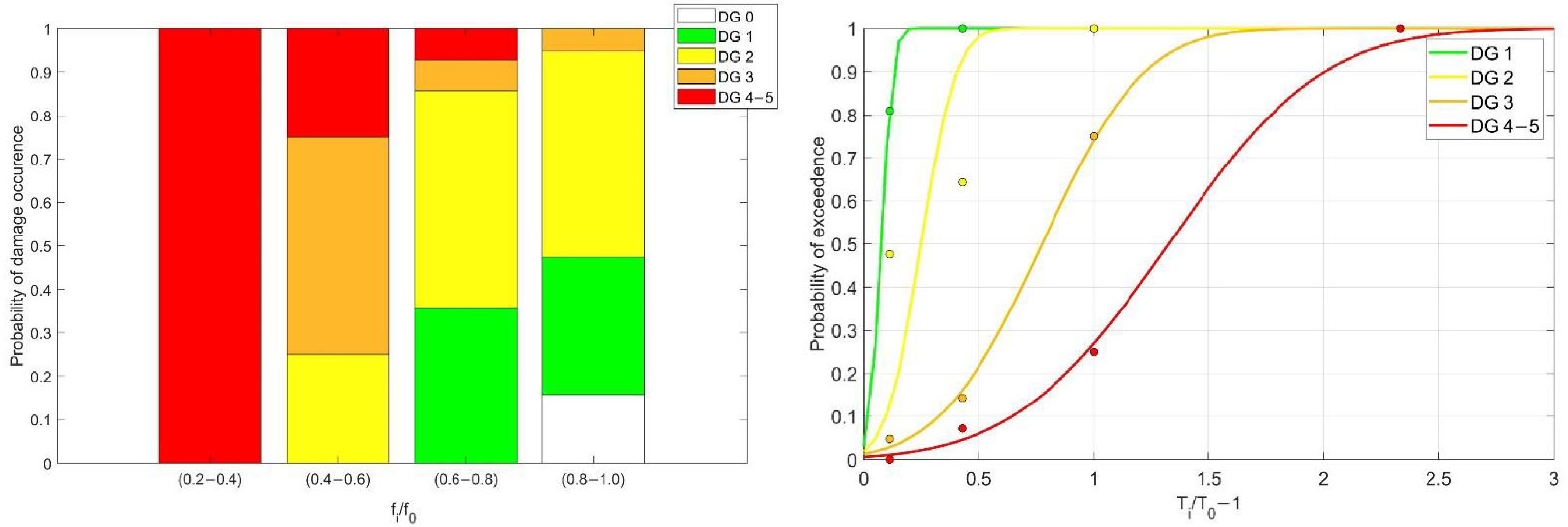
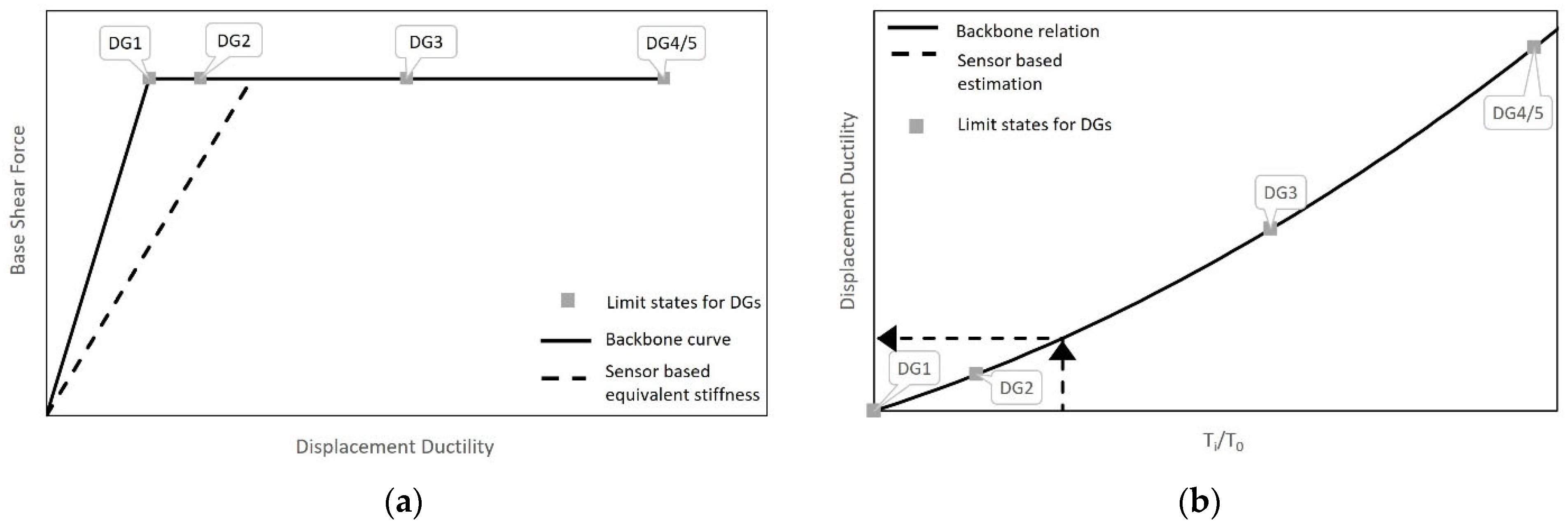
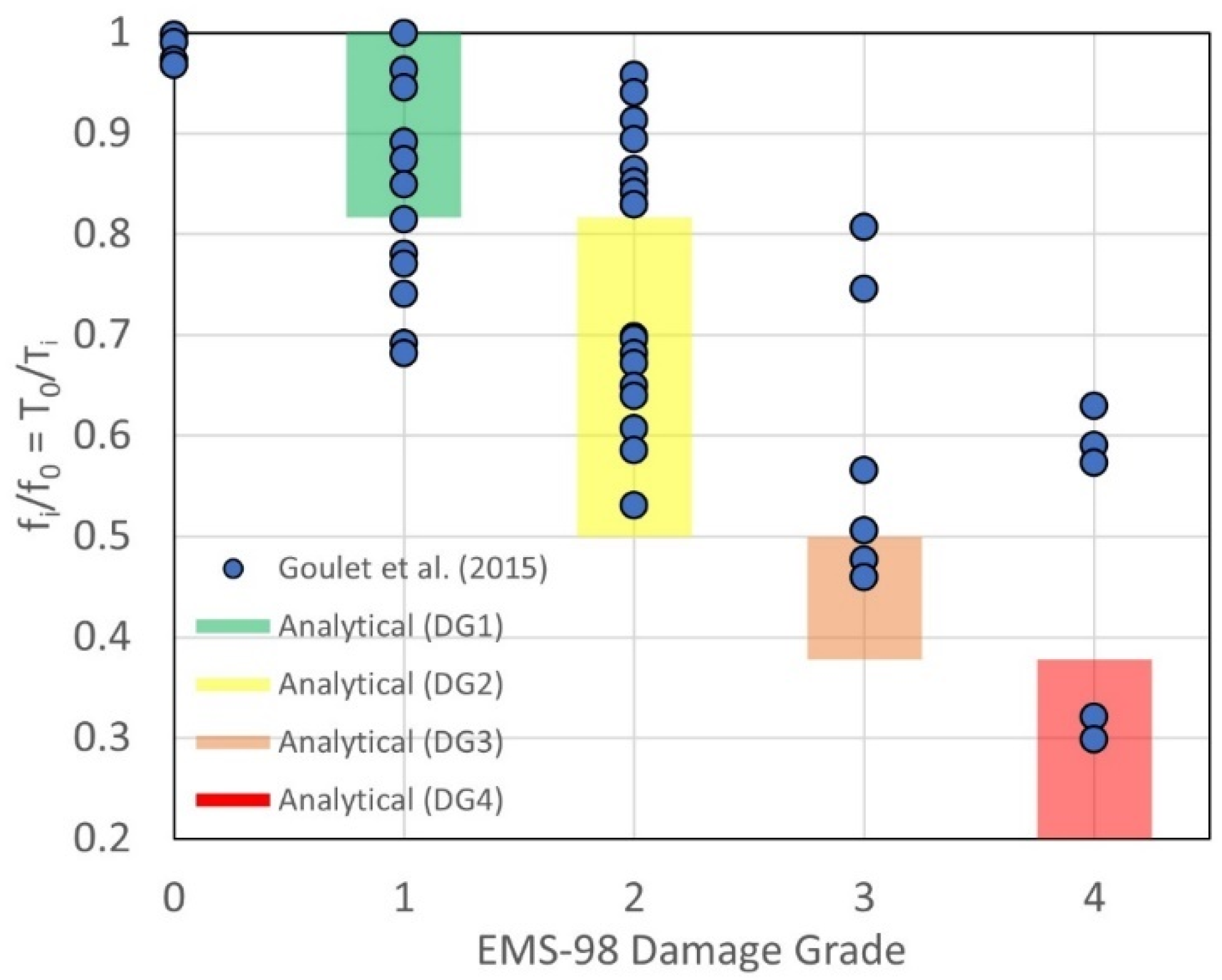
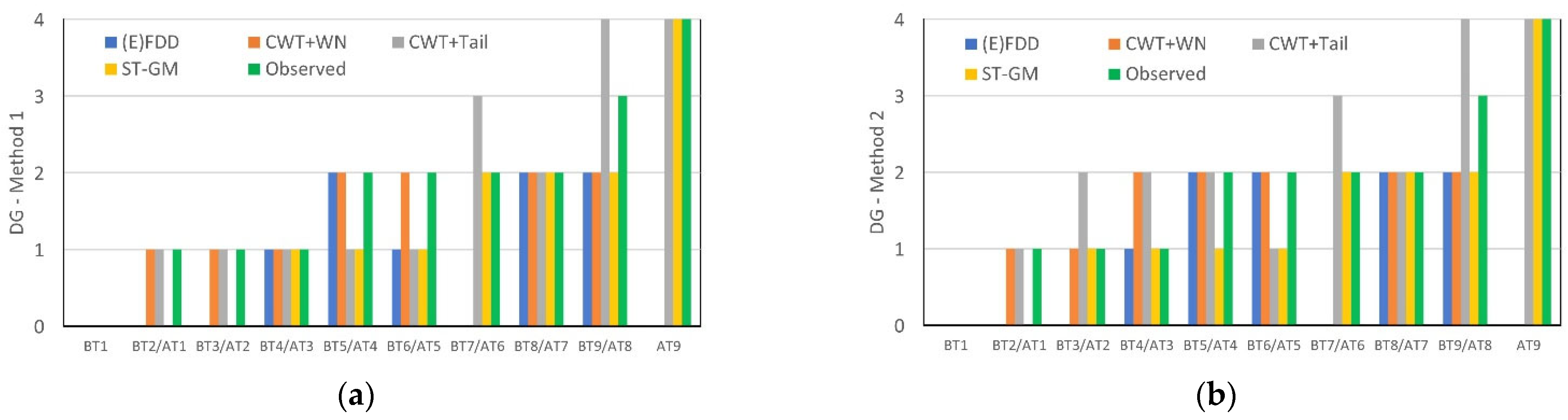
2.2. Overview of Selected Methods for Damage Assessment

Three different approaches are proposed for damage estimation using sensor data (namely empirical, analytical, and numerical approaches), based on the available knowledge levels of the structure (namely basic, intermediate, and comprehensive).
Method 1: Empirical (basic) approach. This approach uses the database of empirical observations presented by Goulet et al. [15]. This database associates the EMS-98 damage grades (DG 1 to 5 and 0 for no damage) with the reduction in the fundamental vibration frequency in a seismic event. The dataset comprises information belonging to a building stock that is mainly composed reinforced concrete structures with some exceptions, such as a brick-steel structure [26]. First, the scatter data presented by Goulet et al. [15] are digitized; then empirical histograms of damage level are created for different intervals of the frequency reduction (fi/f0), where f0 and fi are natural frequencies of vibration before and after the earthquake i (such that fi ≤ f0). Finally, damage functions in terms of the normalised period elongation (Ti/T0-1 being analogous to f0/fi-1, where T is the natural vibration period) are generated using a Gaussian distribution. With this approach, the normalised period elongation—obtained via one of the dynamic identification techniques described in the previous section—can be directly entered into the damage functions to determine the probability of damage exceedance (and occurrence). The histograms and derived damage curves obtained from Goulet et al. [15] are presented in Figure 2. Most of the buildings in the dataset used by Goulet et al. [15] account for reinforced concrete structures.
Method 2: Analytical approach. In this method, the concept of secant stiffness [27] is used to relate the reduction in vibration frequency with the maximum displacement ductility demand experienced by the building under the earthquake (Figure 3), similar to SP-BELA [28]. The approach proposed by Lagomarsino and Giovinazzi’s technique [29] is then employed to link ductility demand and damage grade. The method uses a bilinear load-displacement relation approximation (which requires the intermediate knowledge level for the construction) where the first branch is represented by the elastic stiffness k0, and the ultimate force capacity, denoted as Fy, can be obtained through the product of d y and k 0 .
For any arbitrary secant stiffness, ks (shown with the dashed line in Figure 3), Equation (11) holds true for the displacement ductility demand (μ)
μ = k 0 / k s = ( F y / k s ) / d y
The secant stiffness can be related to the fundamental vibration period through the following relationship:
k 0 , S = m ( 2 π / T 0 , S ) 2
In Equation (12), m denotes the mass, and Ti denotes the identified secant stiffness-compatible period. Combining Equations (11) and (12), one obtains:
μ = ( T i / T 0 ) 2
where T 0 is the period of vibration of the undamaged building.
Assuming the displacement ductility limits of 1.0 (DG1), 1.5 (DG2), 4.0 (DG3), 7.0 (DG4 and 5), one may obtain the following range of values of the T0/Ti (or frequency fi/f0) limit ratios for the different damage grades:
f i f 0 = T 0 T i { 1.00 0.82 f o r   D G 1 0.82 0.50 f o r   D G 2 0.50 0.38 f o r   D G 3             0.38 0 f o r   D G 4   &   5
It is clear that considering different values of the ductility limits would lead to different range of values of T0/Ti. Further details are provided regarding the specific ductility limits adopted for the case study in Section 3.2.
Figure 4 compares the DG interval-frequency ratios of Equation (14), using the empirical data points collected in [15].
Method 3: Numerical approach. This method combines the results of numerical analyses of the structural systems with the results of the application of dynamic identification techniques using sensor data. Drift and ductility limits are used to evaluate the structural performance. Complete and simplified model setups are created within the context of numerical modelling. In the complete model, accurate representations of the geometry, connectivity, and member load-deformation responses are considered. In the case of sequential analyses, a model updating scheme is followed to redefine the stiffness values by updating the material properties between two consecutive events (Figure 5a). The method uses pre-event vibration data to calibrate the model by minimizing the error between actual response and model-generated time history response based on a given ground excitation captured at the base level. For simplified models, calibration terms can be deduced to effective stiffness, while in full-scale, indirect terms such as physical parameters (i.e., Young’s modulus) are parameterized to find the optimal model. For damage assessment, the seismic record is applied to the model to estimate the top roof drift and classify the demand according to the limit states defined above.
With the simplified model, the structure is idealized through a single degree of freedom (SDOF) system with the hysteretic hardening softening (HHS) model [30]. Developed to describe the response of reinforced concrete members/systems, the HHS model is defined by a tri-linear primary curve (i.e., backbone curve for non-softening systems) with associated unloading and reloading curves. The first segment of the backbone curve represents the uncracked elastic stiffness, the second segment indicates the cracked elastic stiffness, and the third segment defines the strength plateau. Unloading and reloading rules consider stiffness degradation due to the increasing number of cycles and the inelastic deformation amplitude. The user input is provided in terms of modal mass and a load-displacement curve. The block diagram for the proposed process is given in Figure 5b.
The relationship between multi-degree-of-freedom (MDOF) displacement quantities and equivalent SDOF values is represented by the following equations.
d * = d / Γ
Γ = φ T M [ 1 ] φ T M φ
In Equations (15) and (16), d and d* are the displacement demands of the MDOF and equivalent SDOF systems, and Γ is the modal participation factor, which could be calculated by using M and first mode shape vector φ , defined according to Equation (17). For an N storey structure with equal floor mass, M is the mass matrix equal to m f l o o r   I N  tons, IN is the N × N identity matrix, and [1] is N × 1 unit vector.
φ = { 1 N , 2 N , , N N } T
In Equation (17), φ is the modal shape vector, which could be assumed as linear for simplicity. Figure 5 presents the flowcharts of detailed and simplified numerical models, where the model interacts with recorded ground motions and is calibrated using a sensor-based initial stiffness formulation.

3. Experimental Setup of a Multi-Story Building

This section introduces the case study considered for evaluating and comparing the damage assessment approaches described in the previous section. The case study consists of a multi-storey building subjected to cumulative seismic damage through a series of seismic shake table tests with increasing earthquake intensity. The building specimen, experimental setup, and test processes are first described. Then, the results of the application of the three damage estimation approaches are presented.

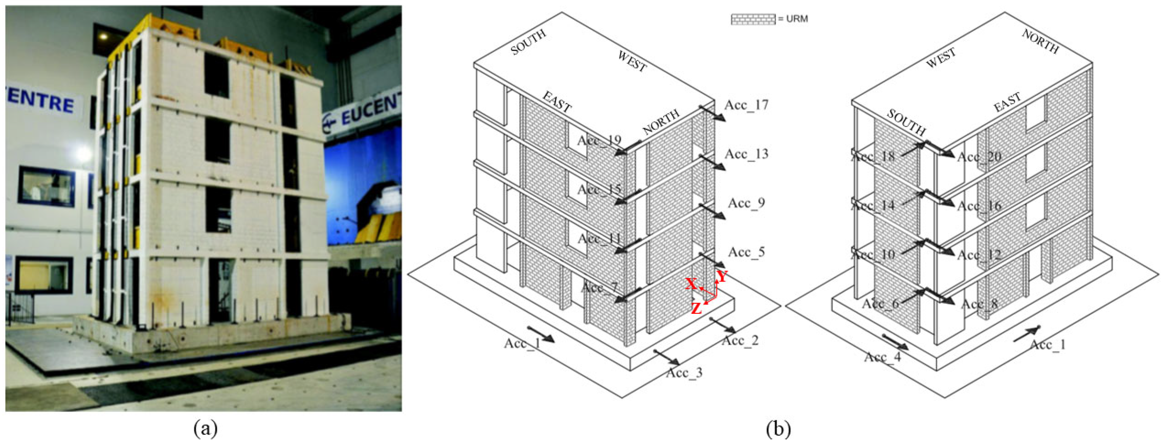
3.1. Experimental Configuration

The case study analysed in this paper is a four-story reinforced dual concrete—unreinforced masonry building subject to uniaxial excitation through shake-table tests performed at the EUCENTRE laboratories [31]. Each story consists of a 1400 mm clear length and a slab thickness of 150 mm. The structural (34.9 t) and externally added masses (34.9 t) sum to 69.8 t. The superstructure, foundation, and steel reinforcement classes are C28/35, C40/50, and B450C, respectively. Representative samples from the concrete and masonry parts are associated with respective elasticity moduli of 24.06 GPa and 5.46 GPa.
The structure is symmetric along the north–south axis, asymmetric along the east-west axis, and has no irregularities in elevation. The shake-table excitations are performed uniaxially in the north–south axis, where north-south walls experience out-of-plane, and east-west walls experience in-plane loading. The table base shear capacity is equal to 1720 kN, and the maximum base shear demand experienced throughout the tests is 757 kN. In summary, the building has a height of 6200 mm and an approximate area of 5560 × 3200 mm2. Figure 6 shows a laboratory view of the testing structure and the sensor configuration for acquiring dynamic response measurements.
The building was instrumented with numerous sensors, including 20 accelerometers that were placed throughout the building (sensor configuration given in Figure 6b). Two types of dynamic tests were conducted, by imposing white noise and earthquake excitations. The earthquake sampling rate was set to 1024 Hz, whereas the white noise excitation sampling rate was set to 256 Hz. White noise was imposed at 0.05 m/s2 amplitude before each earthquake, except in Test 7. Postprocessing included a Butterworth low-pass filter at 40 Hz.
The building was exposed to a repetitive series of input ground motions from the 1979 Montenegro Earthquake (available in the European Strong Motion Database), which were amplified in intensity. The corresponding peak ground acceleration levels investigated were between 0.05 g and 0.9 g, forming nine sequential tests (Figure 7), which lead the building to a state close to collapse from the initial as-built state. Apart from Test 7, white noise excitations were conducted between each earthquake event to indicate the prior/posterior vibration characteristics of the building. Figure 7 presents the consecutive input ground motions, and Table 1 summarizes the ground motion intensities together with measured damage and values of engineering demand parameters (e.g., residual and transient peak drift ratios) taken from [31]. The reader is referred to [32,33,34] for further details on the tests.
This work considers the information presented in [31] as the benchmark both in terms of input (e.g., material properties, reinforcement configuration, load-displacement relation) and output (e.g., Table 1). This is because of the thorough, well-documented nature of the associated experimental campaign and consequent post-processing of results (e.g., compatible frequency identifications through various approaches, crack width measurements, crack pattern photographs, etc.). Inputs from [31] are used to setup the numerical models, and the study’s outputs are used for carrying out thorough comparisons of the output of the approaches listed in Section 2, in terms of dynamic identification, numerical model verification, and damage predictions.

3.2. Limit State Thresholds for the EMS-98 Damage Grades

The structure under consideration is a scaled experimental setup with a unique structural typology. In the reference article [31], bilinearly approximated pushover curves defining the nonlinear character of the structure report an average yield drift of 0.13% and failure drift of 0.90%. According to [29], the limit state thresholds may be defined by considering an ultimate ductility capacity of around seven.
μ = 0.7 ;   r o o f = 0.09 % for   EMS 98   damage   grade   =   1 μ = 1.5 ;   r o o f = 0.20 % for   EMS 98   damage   grade   =   2 μ = 4.0 ;   r o o f = 0.52 % for   EMS 98   damage   grade   =   3 μ = μ u = 7.0 ;   r o o f = 0.90 % for   EMS 98   damage   grade     4

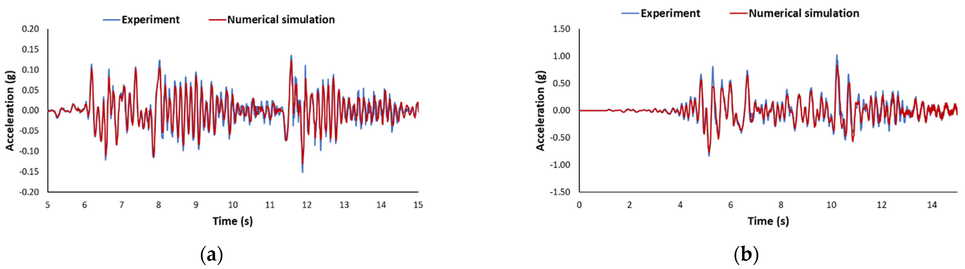
4. Numerical Modelling

4.1. Complete Numerical Modelling

The software platform SeismoStruct 2021 [35] is used to build the numerical model. The test unit’s linear and nonlinear dynamic structural behaviour is described with 2-node frame finite element models. A single inelastic force-based frame element represents RC walls and rectangular beams with effective width. This element is a force-based 3D beam-column element type that is capable of modelling members of space frames with geometric and material nonlinearities. The sectional stress-strain state of beam-column elements is obtained by integrating the nonlinear uniaxial material response of the individual fibres in which the section has been subdivided, fully accounting for the spread of inelasticity along the member length and across the section depth.
An inelastic masonry frame element represents the URM wall. This element is a combination of a 3D, force-based, plastic hinge element type used to primarily model the bending behaviour of the masonry member (herein referred to as the ‘internal sub-element’) and two links at the two edges used to simulate the member’s shear behaviour (herein referred to as the ‘external links’ or ‘link sub-elements’). The internal sub-element and the external links are connected in series, ensuring equilibrium in bending moment and shear force. The only ‘active’ degrees-of-freedom of the link sub-elements are the two translational ones in the shear directions (in-plane and out-of-plane). At the same time, the other four DOFs (axial and three rotational) remain perfectly rigid links. Both masonry walls and spandrels may be precisely simulated with this configuration. The shear DOFs of the link sub-elements feature a hysteretic curve that is based on SeismoStruct’s built-in MIMK-pinched nonlinear curve (Modified Ibarra–Medina–Krawinkler deterioration curve with bilinear hysteretic rules and pinching), which is in accordance with a phenomenological law that describes the shear behaviour of the entire member [36]. Simultaneously, the fibre-section modelling allows for a relatively accurate description of the coupled axial-flexural behaviour in the internal sub-element. The sectional stress-strain state is obtained by integrating the nonlinear uniaxial material response of the individual fibres. The section is subdivided, fully accounting for the spread of inelasticity along the member length across the section depth.
The diaphragm effect of the floor slabs is considered by imposing rigid constraints among all the joints belonging to the same slab. The total construction weight, including the additional weight on the slab, is estimated to be around 676 kN without foundation. The model includes the added weights as lumped masses at the mass centres.
A constant-confinement concrete model ([37,38,39]) is used to represent the nonlinear concrete behaviour. The tensile strength of concrete is neglected, and the confinement effect is described by effective confinement stress, which depends on the longitudinal and transverse reinforcement. The reinforcement steel behaviour is characterized by the uniaxial stress-strain relationship proposed by Menegotto and Pinto [40], coupled with the isotropic hardening rules proposed by Filippou et al. [41].
The time integration is carried out using the Newmark algorithm with γ = 0.5 and β = 0.25 (constant average acceleration method). Convergence is verified for each time step. The convergence criterion is based on displacement and rotation; the maximum values of the ratios between the increments of displacement and rotation (along all the corresponding degrees of freedom), and the prescribed tolerances should be less than or equal to 1. The displacement tolerance is 10−4 m, and the rotation tolerance is 10−4 rad. For the sake of avoiding expensive calculations, the maximum number of iterations is 300 for each time step. The damping matrix is proportional to the initial stiffness; the damping ratio is assumed to be 3.5% for RC members and 7% for masonry walls (based on calibration of the numerical model).
The parameters corresponding to the inelastic masonry frame element are calibrated using the experimental data acquired from the test series of six identical unreinforced masonry walls by Petry and Beyer [42,43]. This experimental campaign comprised of six tests on masonry walls that all had the same dimensions. The walls are named PUP1–6 and represent the first story of the structure tested at the EUCENTRE Laboratories [31]. The test units are subjected to quasi-static cycles of increasing drift demands. The tests differ in terms of the axial load and the moment restraint applied at the top of the walls.
Figure 8 confirms that the estimated parameters resulting from the calibration process for the inelastic masonry frame element can approximately simulate the real behaviour of the URM walls. Further calibrations are conducted based on the structure’s overall behaviour, to complete the development of the numerical model. A nonlinear time history (NLTH) analysis is then conducted on the numerical model, using the input excitation of the shake-table test [31]. The fundamental periods (modal frequencies) are obtained using the classic linear eigenvalue analysis before starting the NLTH analysis, by discretizing the buildings into classical lumped mass models in which the stiffness values of the elements are updated.
Comparisons of measured and calculated top floor acceleration time histories are provided for Test 1 and Test 7 in Figure 9.

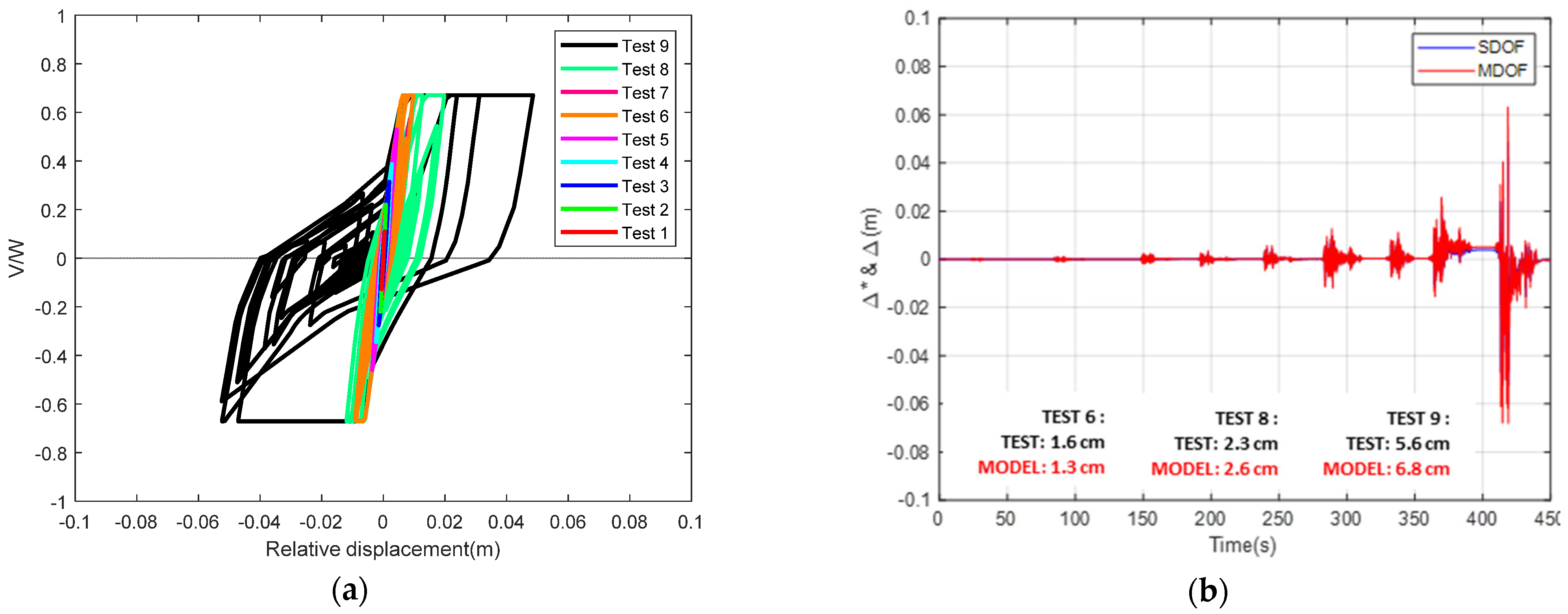
4.2. Simplified Numerical Modelling

In this study, the dynamic load–displacement (i.e., pushover) curve of the MDOF system is directly retrieved from Beyer et al. [31]. Such a curve can be also derived with a simplified approach [28], which is consistent with the KL-2 for the building. In addition to this information, and by setting Γ = 1.3 and reducing the base shear force by 1.3 (consistent to studies of [44,45]), the set of parameters shown in Table 2 is defined to model the equivalent SDOF structure using the HHS model.
The earthquake sequence is applied in the same order as the shake-table tests, without changing any model properties. Figure 10a shows the displacement-normalized base shear response of the SDOF model. Figure 10b compares roof-level lateral displacements obtained using the MDOF extrapolation of the SDOF model (Equation (16)) and those experienced in the experimental campaign for three tests (6, 8, and 9) that resulted in significant accumulation of damage.

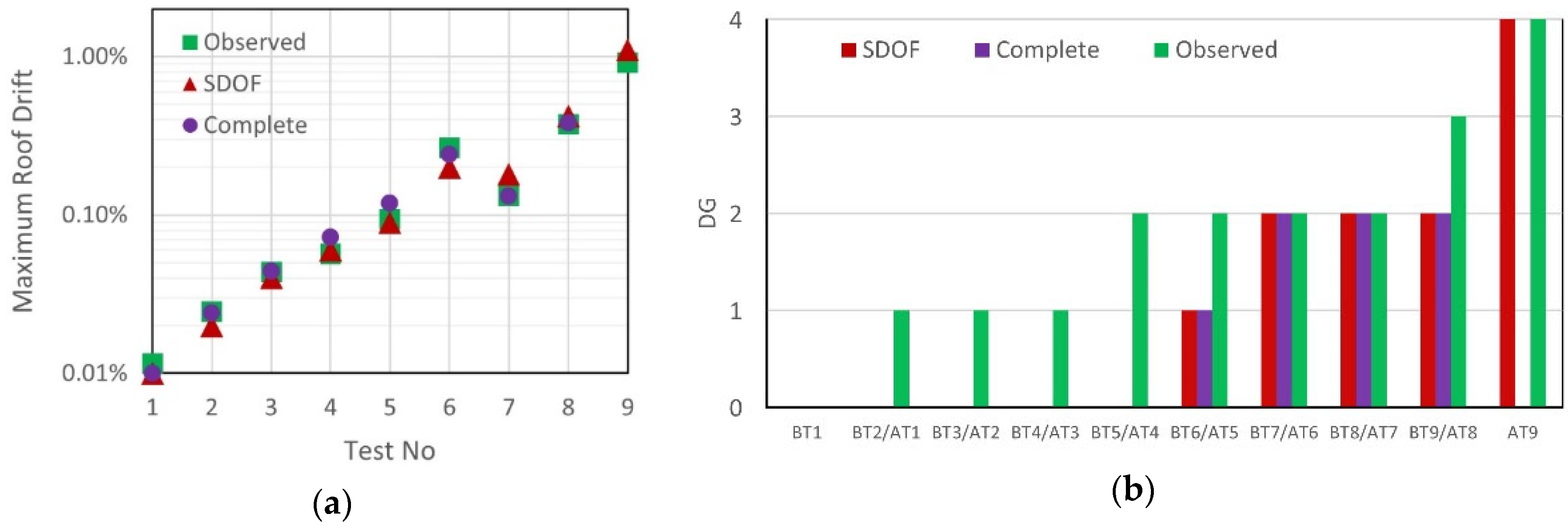
4.3. Damage Estimation through Numerical Modelling

Figure 11 compares the numerical modelling results with the observed experimental results from [31], in terms of maximum roof drifts and damage grades. It is observed that the drift demand is extremely well-captured by both the simplified and complete numerical approaches. On the other hand, damage estimations based on Equation (18) do not demonstrate complete agreement with the corresponding observed data, which may be due to the unique structural typology of the test specimen as well as the sensitive nature of damage initiation. The damage discrepancy is likely to be related to the specific building typology as well as the experimental setup. It is important to note that the damage estimation improves once the structural response becomes moderately non-linear. Hence, it is reasonable to look at the comparison in two phases: (a) the entire test sequence (i.e., Tests 1 to 9) and (b) the strong test sequence yielding visible nonlinearities in the structure (i.e., Tests 6 to 9). While the former sequence ends up with 3/9 and 2/8 accuracy ratios for the simplified modelling and complete modelling approaches, the strong sequence results in 3/4 and 2/3 accuracy ratios. On the other hand, when the damage estimation performance is relaxed to allow for ±1 damage grade accuracy (i.e., allowing for neighbouring grades), the discrepancies of the damage prediction framework disappear for the minor damage range and the predictions become more reliable (i.e., 8/9 for simplified and 7/8 for complete numerical modelling approaches). It should be noted that damage prediction with the complete model for Test 9 is excluded from the comparison due to convergence issues. In any case, the convergence issues reflect a high degree of damage.

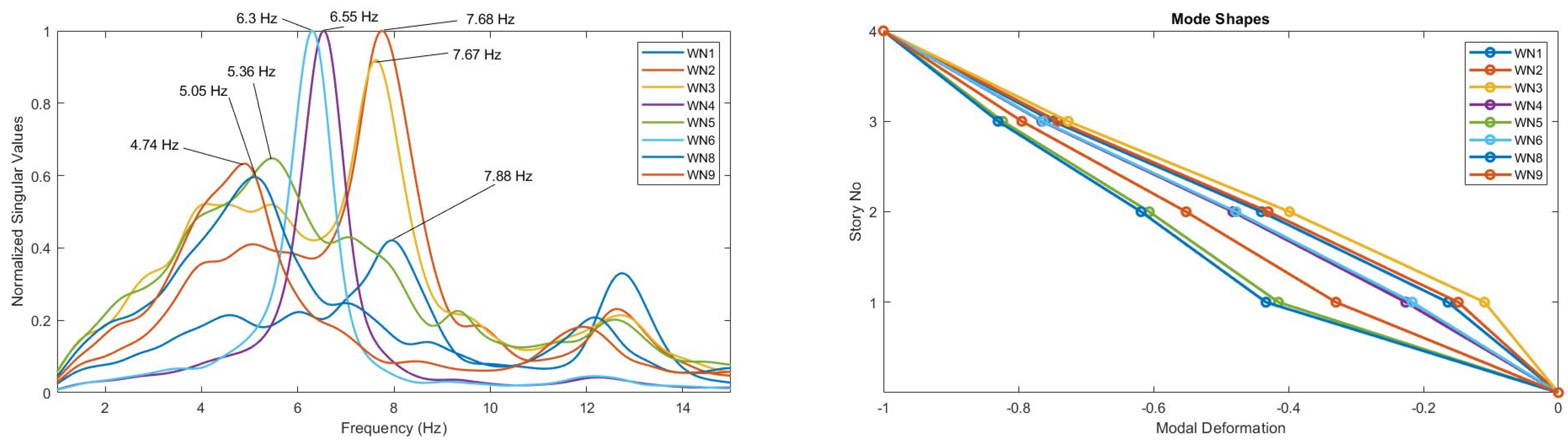
5. Dynamic Identification and Damage Estimation through SHM-Based Approaches

The results of (E)FDD algorithms are presented in Figure 12 in terms of normalized singular values, considering all white noise tests (WN) as well as the illustrative modal shapes from the eigenvectors. Peak singular values show a leftward shift in the frequency domain as a result of a reduction in structural stiffness due to cumulative seismic damage. While there is a change in mode shapes with different states of damage, the pattern is not as indicative as frequency decay, or alternatively, period elongation.
Figure 13 illustrates the results of the wavelet transform approach for Tests 1 and 9. The structural behaviour mode changes during the nine tests and can be explained using the wavelet analysis. From Tests T1 to T3, the structure has the same behaviour and, consequently, one main period is identified. This main period shifts from 0.13 (7.69 Hz) to 0.16 s (6.25 Hz) during the first three tests, which signifies the softening of the structure but not a change in mode response. Periods between 0.22 (4.54 Hz) and 0.39 (2.56 Hz) s are observed for Tests T4 to T9 such that the 0.13 s period disappears; this indicates a change in structural response behaviour due to the occurrence of moderate to significant structural damages.
The results of the S-Transform amplification approach are shown for Tests 6 and 9 in Figure 14. In Test 6, it can be seen that the brittle crack formation in URM walls causes a sudden drop in vibration frequency from about 6.7 Hz to about 5.1 Hz. The damage in the structure is more ductile for Test 9, such that reductions in vibration frequency are more widely distributed over time. The strong motion reduces the oscillation frequency from about 5.0 Hz to about 2.1 Hz. In both cases, the initial vibration frequencies are well in-line with white noise measurements reported in the original article (Beyer et al., 2015).
In Table 3, the results obtained through different methods (WN: (E)FDD/CWT-WN and GM: CWT-Tail/ST-GM) are summarized and compared with the values obtained through white noise (WN) investigations in [31]. All methods replicate the published values of the natural period of vibration acceptably well. Although not conducted here, it is possible to combine these different identification findings in a unified scheme and perform damage detection in an automated manner [46,47].
The damage predictions shown in Figure 15 relate to the use of period elongation, calculated by both empirical (through Figure 2) and analytical approaches (through Equation (14)). The use of sensor-based Ti/T0 together with the empirical and analytical approaches provides reliable estimations of the damage evolution, with some inevitable inaccuracies. However, given the ease and speed of the methods in rapid damage assessment, these inaccuracies could be tolerated. The analytical method particularly tends to give lower bound damage predictions, which may be allocated using a relaxed plus one damage grade assignment scheme during real-life post-disaster evaluations. Moreover, as expected following the discussion of Section 4.3, the accuracy of Method 2 increases with increasing level of nonlinearity in the structural system (i.e., stronger motions present for the Tests 6 to 9).
The results discussed until this point are tabulated in Table 4 in terms of damage prediction performance, considering the entire and nonlinear test sequences, as well as without considering the ±1 DG accuracy limits. Numbers given in Table 4 correspond to the correct identification counts per test sequence. The same accuracy pattern can also be observed in Figure 15 by counting the damage grade matches between the techniques of interest and the reference EMS-98 findings. In summary, empirical and analytical approaches have acceptable performance over the entire sequence and achieve much better accuracy within the more non-linear range. Note that the techniques differ in terms of computational demand, e.g., the first two approaches can make damage estimates within seconds, while the model-based techniques require minutes. For a final recap on the knowledge-adaptive seismic damage assessment framework developed and implemented in this study, Figure 16 provides a conclusive flowchart that constitutes the fundamental output of current research work. According to the scheme, one can choose different identification algorithms depending on conditions related to detection speed and knowledge level (level 1 to 3).
It should be noted that the results presented herein are based on large-scale experimental work within a relatively controlled environment. The proposed work herein is a proof-of-concept to demonstrate that instrumentation data can feed the damage assessment procedure in a rapid and simultaneous way. Shake-table tests provide an opportunity to formulate the proof-of-concept with carefully observed parameters, a multisensory dataset, and accurate damage metrics employed by [31]. In future work, the authors will apply the proposed framework to existing buildings in TURNkey Testbed-1: Bucharest, Romania, using further information provided in [48].

6. Conclusive Remarks

This study proposed different SHM-based approaches for rapid damage assessment of building frames, aimed at complementing (or even avoiding) associated visual inspections and human intervention. The proposed approaches are tailored to different levels of knowledge of the building and offer the possibility to perform either model-driven or model-free damage assessments. SHM-based damage assessment is based on the translation of modal identification results to damage estimates, i.e., the normalised period elongation is used as a proxy of the damage, expressed in terms of EMS-98 damage grades. Three different levels of knowledge are idealized, which respectively correspond to modelling information that is unavailable, available to a limited extent, and fully available. Empirical, analytical, and numerical models with different levels of complexity are proposed to address each of these knowledge levels. A four-story building subjected to large-scale shake-table tests is considered to illustrate application of the methodology and to compare the various approaches for damage assessment. The key findings of the paper can be summarized as follows:
  • Different dynamic identification techniques are consistent in detecting the modal frequencies of the building structure decaying in time due to cumulative seismic damage. This consistency is predominantly reflected in the same EMS-98 damage grade estimations being obtained for each technique.
  • Among different algorithms used in the system identification process, Continuous Wavelet Transform-based damage estimation performed under the white noise domain gives the most accurate damage grade estimation (which is above 85%). However, when the performance is relaxed such that neighbour predicted damage grades are also deemed acceptable, all techniques return 100% detection accuracy for all of the cases.
  • Although estimations with earthquake ground motion (EGM) recordings have relatively lower accuracy compared with white noise, it should be noted that white noise signals are likely unavailable for low-cost accelerometers unless there is a distinct vibration source in the testing vicinity. On the other hand, methods capable of deploying EGM are not affected by noise characteristics and are likely to capture the period elongation even during low-amplitude seismic events.
  • When empirical, analytical, and numerical methods are compared, it is observed that even the KL1 compatible empirical approach performed acceptably well. This constitutes an important practical outcome, as KL1 is the level of knowledge that is most likely to be present for future potential applications. The KL2 compatible analytical method was found to be more consistent with the empirical method since the methods did not show significant variations in terms of their predictive performances. It is noteworthy that although the developed numerical models do not provide any further improvement of accuracy with respect to the analytical method, they could still be required for loss assessment, which requires an estimate of the demand imposed by the earthquake on structural and non-structural components.
In conclusion, SHM and PBEE can be merged in a synergistic environment that considers a hierarchical availability of building knowledge level, adding further flexibility to the damage estimation procedure. In the next stages of this research, the authors will apply the proposed framework to a real-world setting (i.e., several buildings instrumented with low-cost and low-precision devices), to explore the role of signal-to-noise ratio and tails of recorded earthquake signals in identification accuracy.

Author Contributions

Conceptualization, E.O., A.G.Ö., C.N., A.K., B.B., F.B., S.M., S.P. and E.T.; data curation, E.O., A.G.Ö., C.N. and A.K.; formal analysis, E.O., A.G.Ö., C.N., A.K. and B.B.; methodology, E.O., A.G.Ö., C.N., A.K., B.B., F.B., S.M., S.P. and E.T.; project administration, B.B.; resources, B.B. and S.P.; supervision, B.B., S.M., S.P. and E.T.; visualization, E.O., A.G.Ö., C.N., A.K. and F.B.; writing—original draft, E.O., A.G.Ö., C.N. and A.K.; writing—review and editing, E.O., A.G.Ö., C.N., A.K., B.B., F.B., S.M., S.P. and E.T. All authors have read and agreed to the published version of the manuscript.

Funding

This research was funded by European Union’s Horizon 2020 research and innovation programme with the grant number 821046, project TURNkey (Towards more Earthquake-resilient Urban Societies through a Multi-sensor-based Information System enabling Earthquake Forecasting, Early Warning and Rapid Response actions), and the APC was funded by BRGM, EUCENTRE, the University of Alicante, and the University of Strathclyde.

Acknowledgments

This paper is supported by the European Union’s Horizon 2020 research and innovation programme under grant agreement No 821046, project TURNkey (Towards more Earthquake-resilient Urban Societies through a Multi-sensor-based Information System enabling Earthquake Forecasting, Early Warning and Rapid Response actions). Fruitful comments received from Dina D’Ayala from the University College London, Lars Abrahamczyk from the Bauhaus-Universität Weimar, Pierre Gehl from the French Geological Survey (BRGM), Carlo G. Lai from the University of Pavia, and Gemma Cremen from the University College London are gratefully acknowledged.

Conflicts of Interest

The authors declare no conflict of interest.

References

  1. Federal Emergency Management Agency (US) (Ed.) Rapid Visual Screening of Buildings for Potential Seismic Hazards: A Handbook; Government Printing Office: Redwood City, CA, USA, 2017.
  2. De Martino, G.; Di Ludovico, M.; Prota, A.; Moroni, C.; Manfredi, G.; Dolce, M. Estimation of repair costs for RC and masonry residential buildings based on damage data collected by post-earthquake visual inspection. Bull. Earthq. Eng. 2017, 15, 1681–1706. [Google Scholar] [CrossRef]
  3. Kaplan, O.; Kaplan, G. Response Spectra-Based Post-Earthquake Rapid Structural Damage Estimation Approach Aided with Remote Sensing Data: 2020 Samos Earthquake. Buildings 2021, 12, 14. [Google Scholar] [CrossRef]
  4. Zhu, Z.; German, S.; Brilakis, I. Visual retrieval of concrete crack properties for automated post-earthquake structural safety evaluation. Autom. Constr. 2011, 20, 874–883. [Google Scholar] [CrossRef]
  5. Dabove, P.; Di Pietra, V.; Lingua, A.M. Close range photogrammetry with tablet technology in post-earthquake scenario: Sant’Agostino church in Amatrice. GeoInformatica 2018, 22, 463–477. [Google Scholar] [CrossRef]
  6. Dominici, D.; Alicandro, M.; Massimi, V. UAV photogrammetry in the post-earthquake scenario: Case studies in L’Aquila. Geomat. Nat. Hazards Risk 2017, 8, 87–103. [Google Scholar] [CrossRef] [Green Version]
  7. Doebling, S.W.; Farrar, C.R.; Prime, M.B.; Shevitz, D.W. Damage Identification and Health Monitoring of Structural and Mechanical Systems from Changes in Their Vibration Characteristics: A Literature Review (No. LA-13070-MS); Los Alamos National Lab: Los Alamos, NM, USA, 1996. [Google Scholar] [CrossRef] [Green Version]
  8. Rytter, A. Vibrational Based Inspection of Civil Engineering Structures. Ph.D. Thesis, Aalborg University, Aalborg, Denmark, 1993. [Google Scholar]
  9. Uma, S.R. Seismic instrumentation of buildings-A promising step for performance based design in New Zealand. In Proceedings of the NZSEE Conference Proceedings, Palmerston North, New Zealand, 30 March–1 April 2007. [Google Scholar]
  10. Porter, K.; Mitrani-Reiser, J.; Beck, J.L. Near-real-time loss estimation for instrumented buildings. Struct. Des. Tall Spec. Build. 2006, 15, 3–20. [Google Scholar] [CrossRef]
  11. Cremen, G.; Baker, J.W. Quantifying the benefits of building instruments to FEMA P-58 rapid post-earthquake damage and loss predictions. Eng. Struct. 2018, 176, 243–253. [Google Scholar] [CrossRef]
  12. Tubaldi, E.; Ozer, E.; Douglas, J.; Gehl, P. Examining the contribution of near real-time data for rapid seismic loss assessment of structures. Struct. Health Monit. 2021, 21, 118–137. [Google Scholar] [CrossRef]
  13. Hwang, S.-H.; Lignos, D.G. Nonmodel-based framework for rapid seismic risk and loss assessment of instrumented steel buildings. Eng. Struct. 2018, 156, 417–432. [Google Scholar] [CrossRef] [Green Version]
  14. Reuland, Y.; Lestuzzi, P.; Smith, I.F.C. Measurement-based support for post-earthquake assessment of buildings. Struct. Infrastruct. Eng. 2019, 15, 647–662. [Google Scholar] [CrossRef] [Green Version]
  15. Goulet, J.A.; Michel, C.; Der Kiureghian, A. Data-driven post-earthquake rapid structural safety assessment. Earthq. Eng. Struct. Dyn. 2015, 44, 549–562. [Google Scholar] [CrossRef] [Green Version]
  16. Schwarz, J.; Abrahamczyk, L.; Hadidiam, N.; Haweyon, M.; Kaufmann, C. Deliverable D4.1—Report on Knowledge-Based Exposure Modelling Framework Depending on the Accuracy and Completeness of Available Data. EU H2020 TURNkey Project Deliverable. 2021. Available online: https://earthquake-turnkey.eu/deliverables-2/ (accessed on 25 March 2022).
  17. Grunthal, G. (Ed.) European Macroseismic Scale; Chaiers du Centre Européen de Géodynamique et de Séismologie: Luxembourg, 1998; Volume 15. [Google Scholar]
  18. Brincker, R.; Ventura, C.E.; Andersen, P. Damping estimation by frequency domain decomposition. In Proceedings of the 19th Int’l Modal Analysis Conference (IMAC), Kissimmee, FL, USA, 5–8 February 2001; pp. 698–703. [Google Scholar]
  19. Brincker, R.; Zhang, L.; Andersen, P. Modal identification of output-only systems using frequency domain decomposition. Smart Mater. Struct. 2001, 10, 441–445. [Google Scholar] [CrossRef] [Green Version]
  20. Hasan, M.D.A.; Ahmad, Z.A.B.; Leong, M.S.; Hee, L.M. Enhanced frequency domain decomposition algorithm: A review of a recent development for unbiased damping ratio estimates. J. Vibroeng. 2018, 20, 1919–1936. [Google Scholar] [CrossRef]
  21. Stockwell, R.G.; Mansinha, L.; Lowe, R.P. Localization of the complex spectrum: The S transform. IEEE Trans. Signal Process. 1996, 44, 998–1001. [Google Scholar] [CrossRef]
  22. Ditommaso, R.; Mucciarelli, M.; Parolai, S.; Picozzi, M. Monitoring the structural dynamic response of a masonry tower: Comparing classical and time-frequency analyses. Bull. Earthq. Eng. 2012, 10, 1221–1235. [Google Scholar] [CrossRef] [Green Version]
  23. Ditommaso, R.; Ponzo, F.C.; Auletta, G. Damage detection on framed structures: Modal curvature evaluation using Stockwell Transform under seismic excitation. Earthq. Eng. Eng. Vib. 2015, 14, 265–274. [Google Scholar] [CrossRef]
  24. Pianese, G.; Petrovic, B.; Parolai, S.; Paolucci, R. Identification of the nonlinear seismic response of buildings by a combined Stockwell Transform and deconvolution interferometry approach. Bull. Earthq. Eng. 2018, 16, 3103–3126. [Google Scholar] [CrossRef]
  25. Stockwell, R.G. Why use the S transform? In Pseudo-Differential Operators: Partial Differential Equations and Time-Frequency Analysis; Rodino, L., Schulze, B.-W., Wong, M.W., Eds.; Fields Institute Communications Series 52; American Mathematical Society: Providence, RI, USA, 2007; pp. 279–309. [Google Scholar]
  26. Omori, F. The Semi-Destructive Earthquake of April 26; Seismological Notes; Imperial Earthquake Investigation Committee: Tokyo, Japan, 1922; Volume 3, pp. 1–30. [Google Scholar]
  27. Priestley, M.J.N.; Seible, F.; Calvi, G.M. Seismic Design and Retrofit of Bridges; John Wiley & Sons, Inc.: New York, NY, USA, 1996. [Google Scholar]
  28. Borzi, B.; Pinho, R.J.S.M.; Crowley, H. Simplified pushover-based vulnerability analysis for large-scale assessment of RC buildings. Eng. Struct. 2008, 30, 804–820. [Google Scholar] [CrossRef]
  29. Lagomarsino, S.; Giovinazzi, S. Macroseismic and mechanical models for the vulnerability and damage assessment of current buildings. Bull. Earthq. Eng. 2006, 4, 415–443. [Google Scholar] [CrossRef]
  30. Borzi, B.; Calvi, G.M.; Elnashai, A.; Faccioli, E.; Bommer, J. Inelastic spectra for displacement-based seismic design. Soil Dyn. Earthq. Eng. 2001, 21, 47–61. [Google Scholar] [CrossRef]
  31. Beyer, K.; Tondelli, M.; Petry, S.; Peloso, S. Dynamic testing of a four-storey building with reinforced concrete and unreinforced masonry walls: Prediction, test results and data set. Bull. Earthq. Eng. 2015, 13, 3015–3064. [Google Scholar] [CrossRef] [Green Version]
  32. Tondelli, M.; Petry, S.; Beyer, K. Seismic Behaviour of Mixed Reinforced Concrete—Unreinforced Masonry Wall Structures; TREES Laboratory, EUCENTRE: Pavia, Italy, 2013. [Google Scholar]
  33. Tondelli, M.; Petry, S.; Peloso, S.; Beyer, K. Dynamic Testing of a Four-Storey Building with Reinforced Concrete and Unreinforced Masonry Wall: Data Set. 2014. Available online: https://zenodo.org/record/11578 (accessed on 25 March 2022).
  34. Tondelli, M.; Beyer, K.; DeJong, M. Influence of boundary conditions on the out-of-plane response of brick masonry walls in buildings with RC slabs. Earthq. Eng. Struct. Dyn. 2016, 45, 1337–1356. [Google Scholar] [CrossRef] [Green Version]
  35. Seismosoft. SeismoStruct 2021—A Computer Program for Static and Dynamic Nonlinear Analysis of Framed Structures. 2021. Available online: www.seismosoft.com (accessed on 29 March 2022).
  36. Ibarra, L.F.; Medina, R.A.; Krawinkler, H. Hysteretic models that incorporate strength and stiffness deterioration. Earthq. Eng. Struct. Dyn. 2005, 34, 1489–1511. [Google Scholar] [CrossRef]
  37. Mander, J.B.; Priestley, M.J.N.; Park, R. Theoretical Stress-Strain Model for Confined Concrete. J. Struct. Eng. 1988, 114, 1804–1826. [Google Scholar] [CrossRef] [Green Version]
  38. Martínez-Rueda, J.E.; Elnashai, A.S. Confined concrete model under cyclic load. Mater. Struct. 1997, 30, 139–147. [Google Scholar] [CrossRef]
  39. Madas, P. Advanced Modelling of Composite Frames Subjected to Earthquake Loading. Ph.D. Thesis, Imperial College, University of London, London, UK, 1993. [Google Scholar]
  40. Menegotto, M.; Pinto, P.E. Method of analysis for cyclically loaded R.C. plane frames including changes in geometry and non-elastic behaviour of elements under combined normal force and bending. In Proceedings of the Symposium on the Resistance and Ultimate Deformability of Structures Acted on by Well Defined Repeated Loads, International Association for Bridge and Structural Engineering, Zurich, Switzerland, June 1973; pp. 15–22. [Google Scholar] [CrossRef]
  41. Filippou, F.C.; Popov, E.P.; Bertero, V.V. Effects of Bond Deterioration on Hysteretic Behaviour of Reinforced Concrete Joints; Report EERC 83-19; Earthquake Engineering Research Center, University of California: Berkeley, CA, USA, 1983. [Google Scholar]
  42. Petry, S.; Beyer, K. Scaling unreinforced masonry for reduced-scale seismic testing. Bull. Earthq. Eng. 2014, 12, 2557–2581. [Google Scholar] [CrossRef] [Green Version]
  43. Petry, S.; Beyer, K. Cyclic Test Data of Six Unreinforced Masonry Walls with Different Boundary Conditions. Earthq. Spectra 2015, 31, 2459–2484. [Google Scholar] [CrossRef] [Green Version]
  44. Mwafy, M.; Elnashai, A.S. Static pushover versus dynamic collapse of RC buildings. Eng. Struct. 2001, 23, 407–424. [Google Scholar] [CrossRef]
  45. Louzai, A.; Abed, A. Evaluation of the seismic behavior factor of reinforced concrete frame structures based on comparative analysis between non-linear static pushover and incremental dynamic analyses. Bull. Earthq. Eng. 2015, 13, 1773–1793. [Google Scholar] [CrossRef]
  46. Tran, T.T.X.; Ozer, E. Automated and Model-Free Bridge Damage Indicators with Simultaneous Multiparameter Modal Anomaly Detection. Sensors 2020, 20, 4752. [Google Scholar] [CrossRef]
  47. Tran, T.T.; Ozer, E. Synergistic bridge modal analysis using frequency domain decomposition, observer Kalman filter identification, stochastic subspace identification, system realization using information matrix, and autoregressive exogenous model. Mech. Syst. Signal Process. 2021, 160, 107818. [Google Scholar] [CrossRef]
  48. Tiganescu, A.; Grecu, B.; Neagoe, C.; Toma-Danila, D.; Tataru, D.; Ionescu, C.; Balan, S.F. PREVENT—An Integrated Multi-Sensor System for Seismic Monitoring of Civil Structures. Rom. Rep. Phys. 2021, 73. Available online: http://www.rrp.infim.ro/IP/AP599.pdf (accessed on 29 March 2022).
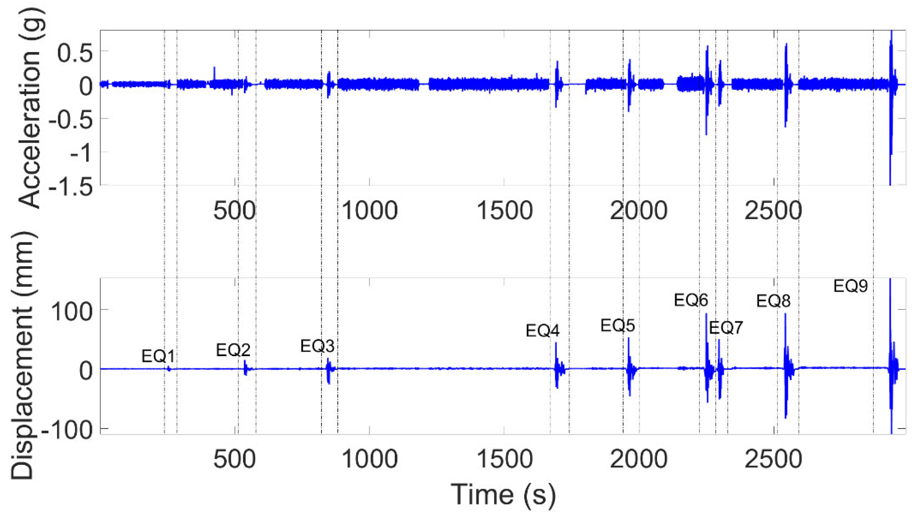
Figure 1. Definitions of knowledge levels, dynamic identification techniques, and KL-dependent damage classification methods.
Buildings 12 00416 g001
Figure 2. Histograms and damage functions based on the empirical data available in Goulet et al. (2015).
Buildings 12 00416 g002
Figure 3. (a) Bi−linear backbone curve and performance evaluation using the secant stiffness concept, (b) Correlation between period elongation and displacement ductility demand.
Buildings 12 00416 g003
Figure 4. Overlap of the ranges of frequency reduction (fi/f0) in terms of EMS-98 DG, computed through the analytical approach (DG1 to DG4) and using data points observed in [15].
Buildings 12 00416 g004
Figure 5. Flowcharts to be followed for (a) complete modelling and (b) simplified modelling.
Buildings 12 00416 g005
Figure 6. Building views: (a) photograph, (b) locations of accelerograms [after Beyer et al., 2015].
Buildings 12 00416 g006
Figure 7. Shake table test input−motion sequence.
Buildings 12 00416 g007
Figure 8. Displacement−force hysteresis for the numerical model and the experiment performed by Petry and Beyer [43] (a) PUP1, (b) PUP2.
Buildings 12 00416 g008
Figure 9. Comparisons of roof level acceleration response histories between the complete numerical model and observed data for (a) Test 1 and (b) Test 7.
Buildings 12 00416 g009
Figure 10. Equivalent SDOF modelling. (a) load−displacement relation, (b) roof displacement response histories.
Buildings 12 00416 g010
Figure 11. Comparison of numerical modelling results in terms of (a) the maximum roof drift ratios, (b) the damage estimations. BT: Before the test, AT: After the test.
Buildings 12 00416 g011
Figure 12. Dynamic identification results using noise−based evaluations from (E)FDD.
Buildings 12 00416 g012
Figure 13. Extracting the wavelet envelope at a natural period Ti for each of the 9 Tests: (Left) all superimposed. (Right) one by one.
Buildings 12 00416 g013
Figure 14. Processing the ground motion data with the approach of ST amplification, considering (a) Test 6 and (b) Test 9. Dark red indicates high intensity response, dark blue indicates low intensity response.
Buildings 12 00416 g014
Figure 15. Damage estimations based on Ti/T0 proxy: (a) Empirical method through Figure 4 and (b) analytical method through Equation (15).
Buildings 12 00416 g015
Figure 16. Proposed flowchart for knowledge level-compatible damage assessment methodology.
Buildings 12 00416 g016
Table 1. Summary of the intensity measure amplitudes and damage observed in each shake-table test.
Test No (EQ)123456789
PGA (g)0.080.130.210.360.410.760.370.641.52
EMS-98 Damage Grade111222234–5
Residual Drift Ratio (%)0.00.00.00.00.00.00.00.00.29
Tr. Drift Ratio, Interstorey (%)0.030.040.080.080.130.330.180.471.39
Tr. Drift Ratio, Roof (%)0.010.020.040.060.090.270.130.370.91
Table 2. Parameters of HHS model.
ParameterDefinitionValue
W*Modal weight581,400 N
F*ySDOF yield strength390,000 N
d*ySDOF yield displacement0.006 m
F*y/F*crThe ratio of yield strength to cracking force3
kplKinematic hardening ratio0
ky/kcrThe ratio of cracked stiffness to uncracked stiffness0.45
Table 3. Comparison of the results of SHM algorithms with published data in terms of the first natural vibration period. BT: Before Test, AT: After Test. * For CWT-Tail: BT1 period is assigned as 0.12 s which is determined by CWT-WN.
Beyer et al. (2015)(E)FDDCWT-WNCWT-TailST-GM
BT10.130.130.120.12 *0.13
AT1 or BT20.130.130.130.140.13
AT2 or BT30.130.130.130.150.14
AT3 or BT40.150.150.150.150.15
AT4 or BT50.160.180.170.150.15
AT5 or BT60.170.160.160.140.15
AT6 or BT7N/AN/AN/A0.270.19
AT7 or BT80.190.210.190.220.18
AT8 or BT90.210.200.200.320.20
AT9N/AN/AN/A0.39 0.48
Table 4. Comparison of EMS-98 DG estimations from empirical, analytical, and numerical methods. DG estimations with ±1 accuracy limits are reported in parenthesis “( )” and italic.
Identification Techniques
Test SequenceTime Required(E)FDDCWT + WNCWT + TailST-GM
Method 1 (Empirical)1 to 9A few seconds3/7 (7/7)6/7 (7/7)5/9 (9/9)4/9 (9/9)
6 to 9 1/2 (2/2)1/2 (2/2)2/4 (4/4)3/4 (4/4)
Method 2 (Analytical)1 to 9A few seconds4/7 (7/7)5/7 (7/7)4/9 (9/9)5/9 (9/9)
6 to 91/2 (2/2)1/2 (2/2)2/4 (4/4)3/4 (4/4)
Modelling Techniques
Test SequenceTime Required SDOFComplete
Method 3 (Numerical)1 to 9 SDOF: About one minute 3/9 (8/9)2/8 (8/8)
6 to 9Complete: Minutes to tens of minutes 3/4 (4/4)2/3 (3/3)
Publisher’s Note: MDPI stays neutral with regard to jurisdictional claims in published maps and institutional affiliations.

