
Generating Inclusive Health Benefits from Urban Green Spaces: An Empirical Study of Beijing Olympic Forest Park


Abstract
:1. Introduction
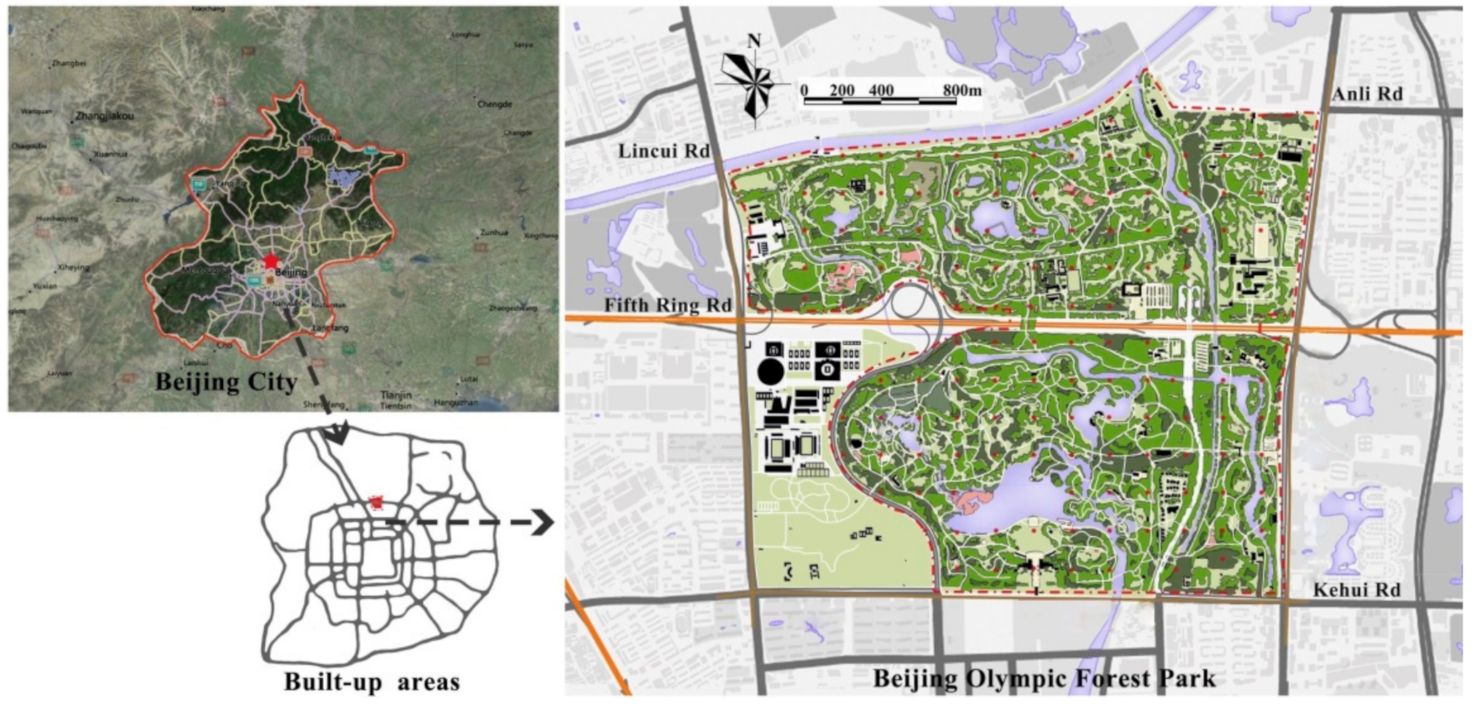
2. Study Area
3. Research Design and Methods
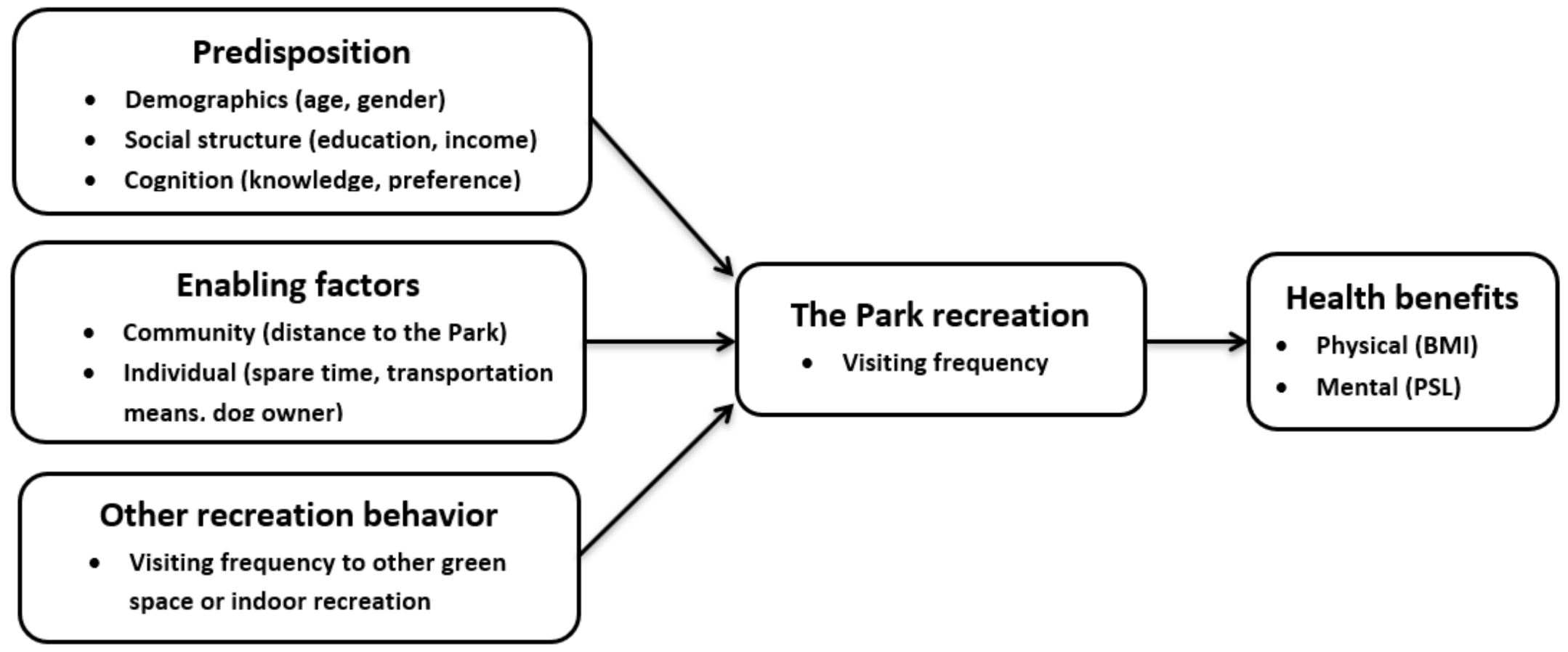
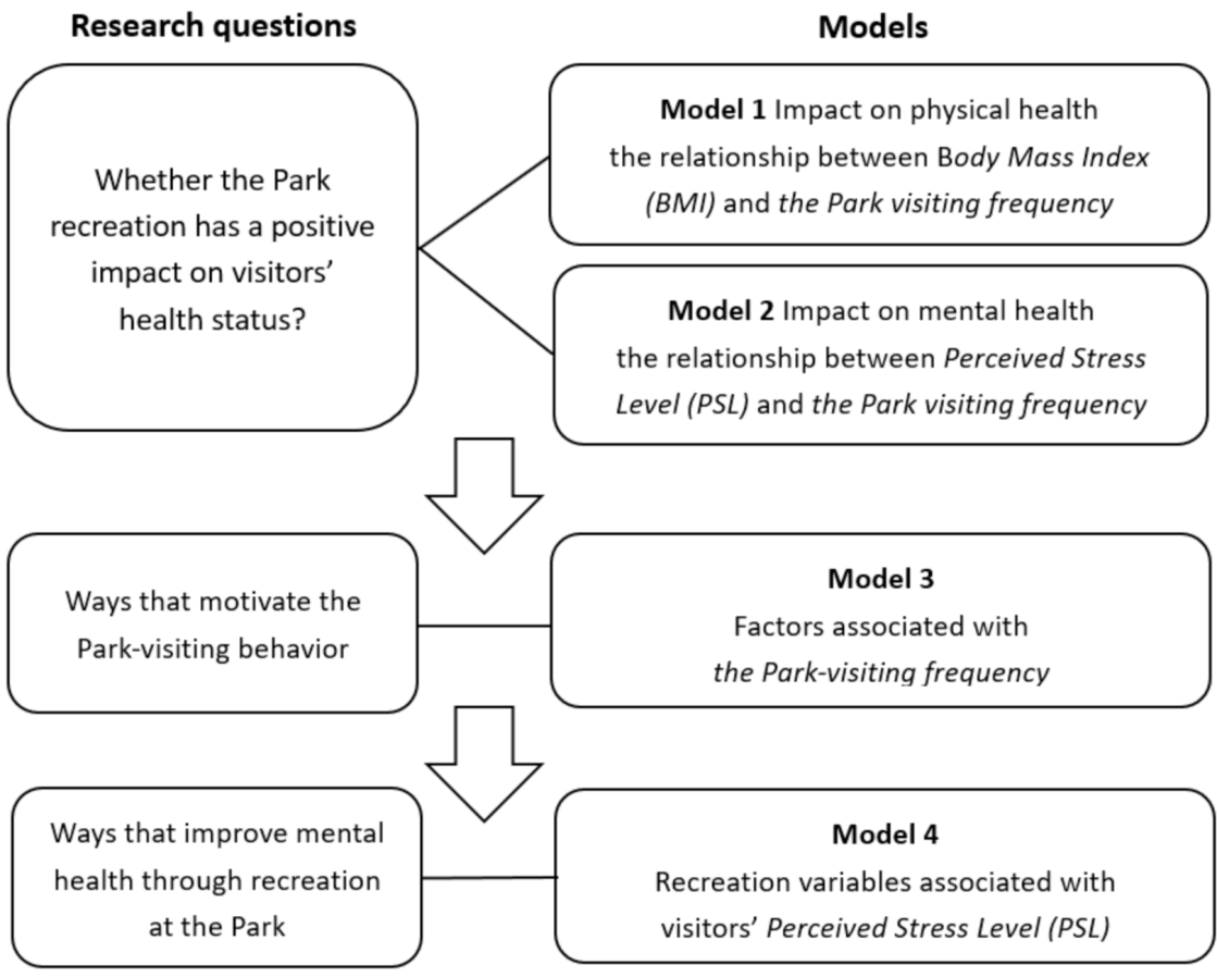
3.1. Conceptual Framework
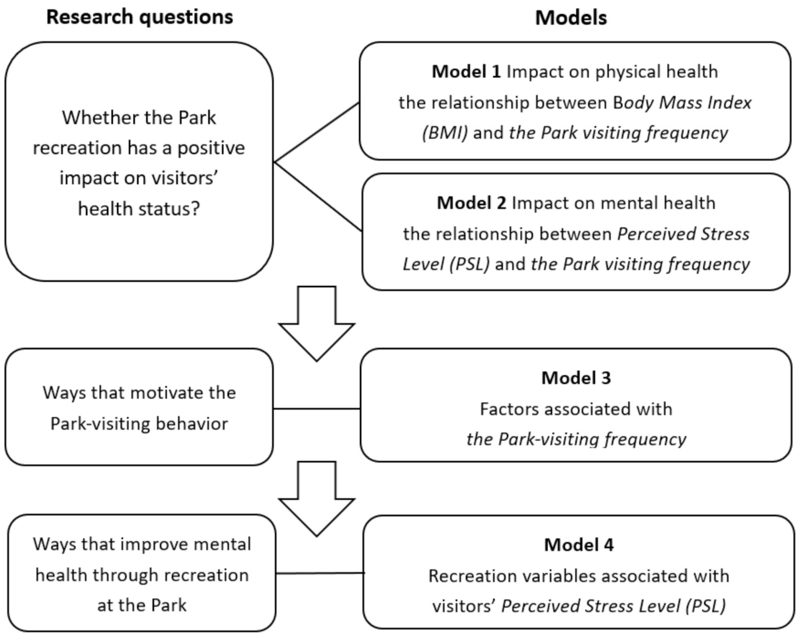
3.1.1. Econometric Models
3.1.2. Questionnaire Design
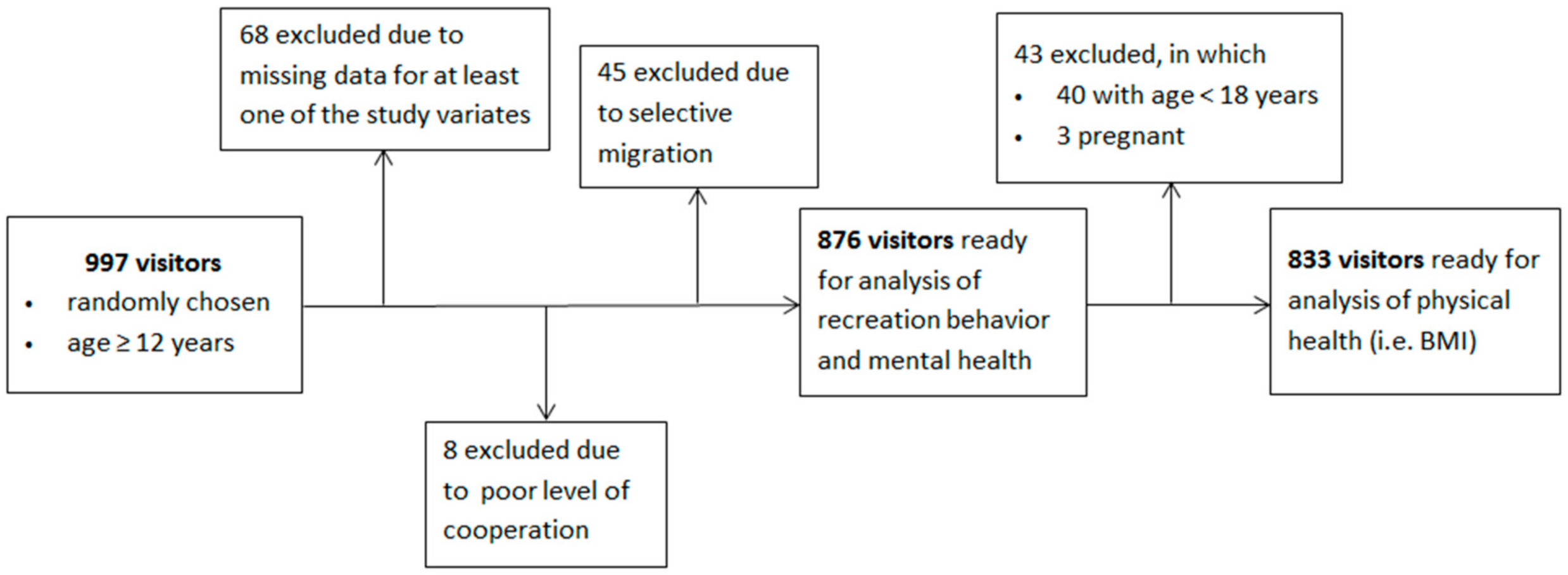
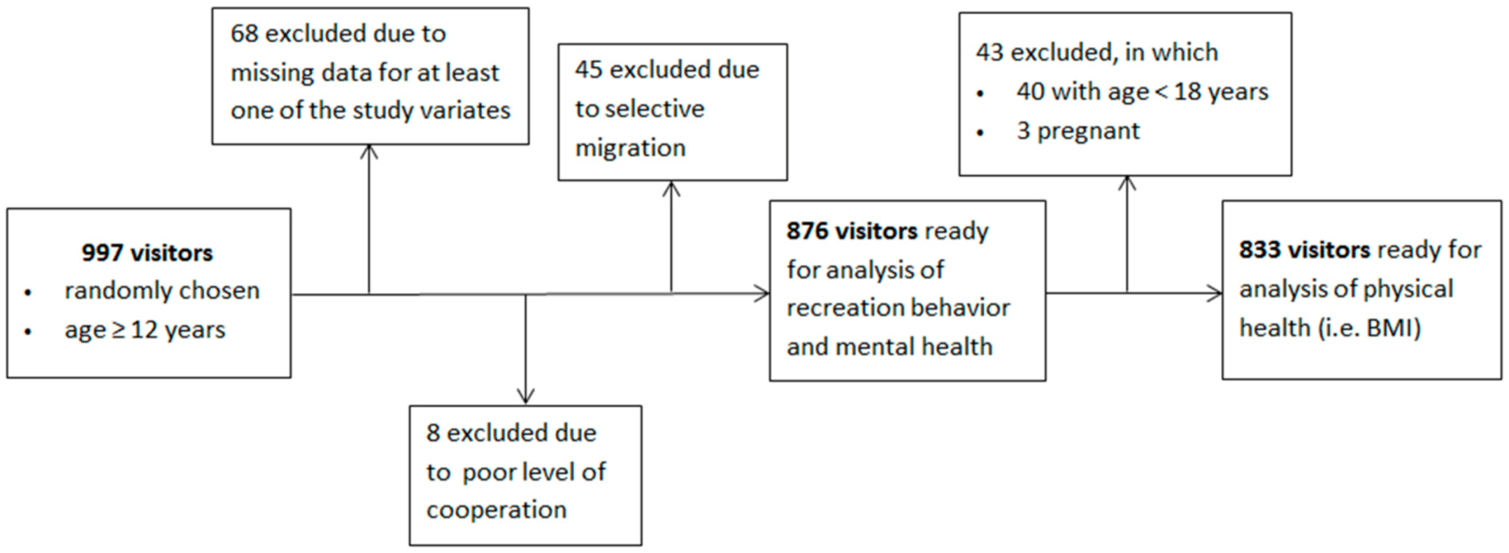
3.1.3. Sampling and Data Collection
3.2. Data Pre-Processing and the Sample Profile
3.3. Data Analysis
4. Results
4.1. Relationship between Physical Health and the Park Visits
4.2. Relationship between Mental Health and the Park Visits
4.3. Correlates of the Park Visits
4.4. Correlates of PSL
5. Discussion
6. Conclusions
Author Contributions
Funding
Institutional Review Board Statement
Informed Consent Statement
Data Availability Statement
Conflicts of Interest
References
- Wohig-Bennett, C.; Jones, A. The Health Benefits of the Great Outdoors: A Systematic Review and Meta-Analysis of Greenspace Exposure and Health Outcomes. Environ. Res. 2018, 166, 628–637. [Google Scholar] [CrossRef] [PubMed]
- van den Bosch, M.; Bird, W. Oxford Textbook of Nature and Public Healththe Role of Nature in Improving the Health of a Population: The Role of Nature in Improving the Health of a Population; Oxford University Press: Oxford, UK, 2018. [Google Scholar]
- Ellaway, A.; Macintyre, S.; Bonnefoy, X. Graffiti, greenery, and obesity in adults: Secondary analysis of European cross sectional survey. BMJ 2005, 331, 611–612. [Google Scholar] [CrossRef] [PubMed] [Green Version]
- West, S.T.; Shores, K.A.; Mudd, L.M. Association of Available Parkland, Physical Activity, and Overweight in America’s Largest Cities. J. Public Health Manag. Pract. 2012, 18, 423–430. [Google Scholar] [CrossRef] [PubMed]
- Coutts, C.; Horner, M.; Chapin, T. Using geographical information system to model the effects of green space accessibility on mortality in Florida. Geocarto Int. 2010, 25, 471–484. [Google Scholar] [CrossRef]
- Richardson, E.A.; Mitchell, R. Gender differences in relationships between urban green space and health in the United Kingdom. Soc. Sci. Med. 2010, 71, 568–575. [Google Scholar] [CrossRef] [PubMed] [Green Version]
- Richardson, E.; Pearce, J.; Mitchell, R.; Kingham, S. Role of physical activity in the relationship between urban green space and health. Public Health 2013, 127, 318–324. [Google Scholar] [CrossRef] [Green Version]
- Van Den Berg, A.E.; Maas, J.; Verheij, R.A.; Groenewegen, P.P. Green space as a buffer between stressful life events and health. Publisher’ s PDF, also known as Version of record Publication date: Social Science & Medicine Green space as a buffer between stressful life events and health. Soc. Sci. Med. 2010, 70, 1203–1210. [Google Scholar] [CrossRef] [Green Version]
- Nutsford, D.; Pearson, A.; Kingham, S. An ecological study investigating the association between access to urban green space and mental health. Public Health 2013, 127, 1005–1011. [Google Scholar] [CrossRef]
- White, M.P.; Alcock, I.; Wheeler, B.W.; Depledge, M.H. Would You Be Happier Living in a Greener Urban Area? A Fixed-Effects Analysis of Panel Data. Psychol. Sci. 2013, 24, 920–928. [Google Scholar] [CrossRef]
- Takano, T.; Nakamura, K.; Watanabe, M. Urban residential environments and senior citizens' longevity in megacity areas: The importance of walkable green spaces. J. Epidemiol. Community Health 2002, 56, 913–918. [Google Scholar] [CrossRef] [Green Version]
- Hartig, T.; Evans, G.W.; Jamner, L.D.; Davis, D.S.; Gärling, T. Tracking restoration in natural and urban field settings. J. Environ. Psychol. 2003, 23, 109–123. [Google Scholar] [CrossRef]
- Ottosson, J.; Grahn, P. A Comparison of Leisure Time Spent in a Garden with Leisure Time Spent Indoors: On Measures of Restoration in Residents in Geriatric Care. Landsc. Res. 2005, 30, 23–55. [Google Scholar] [CrossRef]
- Barton, J.; Pretty, J. What is the Best Dose of Nature and Green Exercise for Improving Mental Health? A Multi-Study Analysis. Environ. Sci. Technol. 2010, 44, 3947–3955. [Google Scholar] [CrossRef] [PubMed]
- Mitchell, R.; Popham, F. Effect of exposure to natural environment on health inequalities: An observational population study. Lancet 2008, 372, 1655–1660. [Google Scholar] [CrossRef] [Green Version]
- Hartig, T.; Mitchell, R.; Vries, S.D.; Frumkin, H. Nature and Health. Annu. Rev. Public Health 2014, 35, 207–228. [Google Scholar] [CrossRef] [PubMed] [Green Version]
- Branas, C.C.; Cheney, R.A.; Macdonald, J.M.; Tam, V.W.; Jackson, T.D.; Ten Have, T.R. A Difference-in-Differences Analysis of Health, Safety, and Greening Vacant Urban Space. Am. J. Epidemiol. 2011, 174, 1296–1306. [Google Scholar] [CrossRef] [PubMed] [Green Version]
- Veitch, J.; Ball, K.; Crawford, D.; Abbott, G.R.; Salmon, J. Park Improvements and Park Activity: A Natural Experiment. Am. J. Prev. Med. 2012, 42, 616–619. [Google Scholar] [CrossRef] [Green Version]
- Tsigos, C.; Chrousos, G.P. Hypothalamic–Pituitary–Adrenal Axis, Neuroendocrine Factors and Stress. J. Psychosom. Res. 2002, 53, 865–871. [Google Scholar] [CrossRef] [Green Version]
- Li, L.; Power, C.; Kelly, S.; Kirschbaum, C.; Hertzman, C. Life-time socio-economic position and cortisol patterns in mid-life. Psychoneuroendocrinology 2007, 32, 824–833. [Google Scholar] [CrossRef]
- Wan, C.; Shen, G.Q.; Choi, S. Underlying relationships between public urban green spaces and social cohesion: A systematic literature review. City Cult. Soc. 2021, 24, 100383. [Google Scholar] [CrossRef]
- Hunter, R.; Cleland, C.; Cleary, A.; Droomers, M.; Wheeler, B.; Sinnett, D.; Nieuwenhuijsen, M.; Braubach, M. Environmental, health, wellbeing, social and equity effects of urban green space interventions: A meta-narrative evidence synthesis. Environ. Int. 2019, 130, 104923. [Google Scholar] [CrossRef] [PubMed]
- He, J.; Yi, H.; Liu, J. Urban green space recreational service assessment and management: A conceptual model based on the service generation process. Ecol. Econ. 2016, 124, 59–68. [Google Scholar] [CrossRef]
- National Bureau of Statistics. China City Statistical Yearbook 2014; National Bureau of Statistics: Beijing, China, 2015. [Google Scholar]
- Wooldridge, J.M. Econometric Analysis of Cross Section and Panel Data; MIT Press: Cambridge, MA, USA, 2002. [Google Scholar]
- Greene, W.H. Econometric Analysis, 6th ed.; Prentice Hall: Upper Saddle River, NJ, USA, 2008. [Google Scholar]
- Giles-Corti, B.; Broomhall, M.H.; Knuiman, M.; Collins, C.; Douglas, K.; Ng, K.; Lange, A.; Donovan, R.J. Increasing Walking: How Important Is Distance to, Attractiveness, and Size of Public Open Space? Am. J. Prev. Med. 2005, 28 (Suppl. S2), 169–176. [Google Scholar] [CrossRef] [PubMed]
- Cohen, D.A.; McKenzie, T.L.; Sehgal, A.; Williamson, S.; Golinelli, D.; Lurie, N. Contribution of Public Parks to Physical Activity. Am. J. Public Health 2007, 97, 509–514. [Google Scholar] [CrossRef] [PubMed]
- Coombes, E.; Jones, A.P.; Hillsdon, M. The relationship of physical activity and overweight to objectively measured green space accessibility and use. Soc. Sci. Med. 2010, 70, 816–822. [Google Scholar] [CrossRef] [Green Version]
- Cohen, S.; Kamarck, T.; Mermelstein, R. A Global Measure of Perceived Stress. J. Health Soc. Behav. 1983, 24, 385–396. [Google Scholar] [CrossRef] [PubMed]
- Warttig, S.L.; Forshaw, M.J.; South, J.; White, A. New, normative, English-sample data for the Short Form Perceived Stress Scale (PSS-4). J. Health Psychol. 2013, 18, 1617–1628. [Google Scholar] [CrossRef]
- Grahn, P.; Stigsdotter, U.A. Landscape planning and stress. Urban For. Urban Green 2003, 2, 1–18. [Google Scholar] [CrossRef] [Green Version]
- Lin, B.; Fuller, R.; Bush, R.; Gaston, K.J.; Shanahan, D.F. Opportunity or Orientation? Who Uses Urban Parks and Why. PLoS ONE 2014, 9, e87422. [Google Scholar] [CrossRef] [Green Version]
- Cohen, D.A.; Ashwood, J.S.; Scott, M.M.; Overton, A.; Evenson, K.R.; Staten, L.K.; Porter, D.; McKenzie, T.L.; Catellier, D. Public Parks and Physical Activity Among Adolescent Girls. Pediatrics 2006, 118, e1381–e1389. [Google Scholar] [CrossRef] [Green Version]
- Wendel, H.E.W.; Zarger, R.K.; Mihelcic, J.R. Accessibility and usability: Green space preferences, perceptions, and barriers in a rapidly urbanizing city in Latin America. Landsc. Urban Plan. 2012, 107, 272–282. [Google Scholar] [CrossRef]
- Jennings, V.; Larson, L.; Yun, J. Advancing Sustainability through Urban Green Space: Cultural Ecosystem Services, Equity, and Social Determinants of Health. Int. J. Environ. Res. Public Health 2016, 13, 196. [Google Scholar] [CrossRef] [PubMed] [Green Version]
- Rigolon, A.; Toker, Z.; Gasparian, N. Who has more walkable routes to parks? An environmental justice study of Safe Routes to Parks in neighborhoods of Los Angeles. J. Urban Aff. 2018, 40, 576–591. [Google Scholar] [CrossRef]


| Variable | Explanation |
|---|---|
| Body Mass Index (BMI) | Calculated by the weight in kilograms divided by the square of the height in meters (kg/m2). Four BMI categories were employed using cutoffs suggested by PRC’s Criteria of Weight for Adults (S/T428-2013): underweight (BMI < 18.5), normal (18.5 ≤ BMI < 24), overweight (24.0 ≤ BMI < 28.0), and obesity (BMI ≥ 28.0). |
| Perceived Stress Level (PSL) | Assessed by the simplified Perceived Stress Scale proposed by Cohen et al. [30] and widely used and validated afterward [31], that provides a validated 4-item instrument measuring how unpredictable, uncontrollable, unhandleable, or overwhelmed people felt their lives were during the past month *. It has a range from 0 to 16, and higher scores indicate more perceived stress. |
| The Park-visiting frequency | Respondents were asked to recall how many times they had visited the Park in the past 28 days. |
| Distance to the Park | The number of kilometers from the respondents’ departure place to the nearest entrance to the Park, calculated by the commercial map navigation software AutoNavi. |
| Other urban green space-visiting frequency | How often respondents visited UGS other than the Park, calculated by adding up the number of visits to other parks and the number of visits to community green space over the past 28 days. |
| Indoor recreation frequency | How many times respondents participated in indoor recreation in the past 28 days. |
| Spare time | The number of hours respondents were free to spend in the past week, excluding time spent eating, sleeping, and doing housework. It was obtained by asking respondents to recall the length of such spare time they spent on both working- and non-working days each week and then adding up the two. |
| Knowledge | The degree to which respondents acknowledge the possible health benefits of UGS recreation, assessed by the number of agreed items of a list of 4 statements of possible health benefits. |
| Preference | Respondents’ preference to UGS recreation, obtained by asking ‘generally, how much do you feel like going to UGS for recreation?’, with options provided as “very high”, “high”, “so so”, “not much”, and “almost none”. |
| Ways of transportation | The kind of transportation respondents usually takes to get to the Park. Options included “walking”, “cycling”, “public transport (bus or subway)”, and “private car or taxi”. |
| Duration | Average length of stay in the Park. |
| Type of activity | The types of recreation activities undertaken in the Park. Options included “jogging”, “other aerobic exercise”, and “other general activities”. |
| Companion | Whether respondents are usually accompanied when going to the Park. |
| Time of regular visit | The length of time since respondents started visiting the Park regularly. Options included “irregular visit”, “1–2 months”, “3–6 months”, “7–12 months”, “1–3 years”, and “4–6 years”. |
| Dog owner | Whether respondents had a pet dog. This was considered as no pet dogs were allowed in the Park. |
| Entrances | Primary | Secondary | Total | ||||
|---|---|---|---|---|---|---|---|
| A | B | C | D | E | F | ||
| Number of visitors sampled | 632 | 80 | 81 | 145 | 32 | 27 | 997 |
| Number | Share (%) | Number | Share (%) | ||
|---|---|---|---|---|---|
| Gender | Was of transportation | ||||
| female | 401 | 45.8 | walking | 167 | 19.1 |
| male | 475 | 54.2 | cycling | 52 | 5.9 |
| Age | subway/bus | 503 | 57.4 | ||
| 12~17 | 43 | 4.9 | private car/taxi | 154 | 17.6 |
| 18~29 | 343 | 39.2 | Companion | ||
| 30~39 | 209 | 23.9 | alone | 266 | 30.4 |
| 40~49 | 109 | 12.4 | with companion | 610 | 69.6 |
| 50~59 | 79 | 9.0 | Type of activity | ||
| 60~69 | 77 | 8.8 | jogging | 259 | 29.6 |
| ≥70 | 16 | 1.8 | other acrobatic exercises | 166 | 18.9 |
| Education | other general activities | 451 | 51.5 | ||
| below bachelor | 223 | 25.5 | Duration | ||
| bachelor | 482 | 55.0 | ≤1 h | 114 | 13.0 |
| above bachelor | 171 | 19.5 | 1–2 h | 305 | 34.8 |
| Income | 2–4 h | 346 | 39.5 | ||
| 0~2999 | 266 | 30.4 | 4–8 h | 108 | 12.3 |
| 3000~4999 | 216 | 24.7 | >8 h | 3 | 0.4 |
| 5000~7999 | 207 | 23.6 | Time of regular visit | ||
| 8000~9999 | 67 | 7.6 | irregular visit | 257 | 29.3 |
| 10,000~14,999 | 77 | 8.8 | 1–2 months | 143 | 16.3 |
| 15,000~19,999 | 23 | 2.6 | 3–6 months | 114 | 13.0 |
| 20,000~29,999 | 15 | 1.7 | 7–12 months | 93 | 10.6 |
| ≥30,000 | 5 | 0.6 | 1–3 years | 172 | 19.7 |
| The Park-visiting frequency in the past 28 days | 4–6 years | 97 | 11.1 | ||
| Once | 326 | 37.2 | Other green space-visiting frequency in the past 28 days | ||
| 2–4 times | 284 | 32.4 | none | 265 | 30.2 |
| 5–8 times | 87 | 10.0 | 1–16 times | 373 | 42.6 |
| 9–16 times | 100 | 11.4 | 17–28 times | 131 | 15.0 |
| 17–27 times | 19 | 2.2 | >28 times | 107 | 12.2 |
| 28 times | 60 | 6.8 | Indoor recreation frequency in the past 28 days | ||
| Distance to the Park | none | 556 | 63.5 | ||
| ≤3 km | 208 | 23.8 | 1–16 times | 302 | 34.5 |
| 3–5 km | 130 | 14.8 | 17–28 times | 18 | 2.0 |
| 5–10 km | 247 | 28.2 | |||
| 10–30 km | 262 | 29.9 | |||
| 30–60 km | 27 | 3.1 | |||
| >60 km | 2 | 0.2 | |||
| Coef. | Robust SE | z Value | p-Value | 95% Conf. Interval | ||
|---|---|---|---|---|---|---|
| The Park-visiting frequency | −0.024 | 0.014 | −1.71 | 0.088 | −0.051 | 0.003 |
| Other urban green space-visiting frequency | −0.007 | 0.005 | −1.42 | 0.155 | −0.018 | 0.003 |
| Indoor recreation frequency | 0.073 | 0.039 | 1.87 | 0.061 | −0.003 | 0.149 |
| Male | 1.427 | 0.749 | 1.90 | 0.057 | −0.041 | 2.895 |
| Age group | 0.000 ** | |||||
| 18~29 (benchmark) | / | / | / | / | / | / |
| 30~39 | 1.766 | 0.950 | 1.86 | 0.063 | −0.096 | 3.629 |
| 40~49 | 1.937 | 1.040 | 1.86 | 0.063 | −0.102 | 3.975 |
| 50~59 | 1.947 | 1.016 | 1.92 | 0.055 | −0.044 | 3.939 |
| 60~69 | 2.785 | 1.625 | 1.71 | 0.087 | −0.400 | 5.970 |
| ≥70 | −12,230.5 | 417.55 | −29.29 | 0.000 | −13,048.8 | −11,412.1 |
| Education level | 0.028 * | |||||
| Below bachelor (benchmark) | / | / | / | / | / | / |
| Bachelor | −2.138 | 1.166 | −1.83 | 0.067 | −4.424 | 0.148 |
| Above bachelor | −1.679 | 0.924 | −1.82 | 0.069 | −3.491 | 0.132 |
| Income group | 0.000 ** | |||||
| 0~2999 (benchmark) | / | / | / | / | / | / |
| 3000~4999 | 0.990 | 0.852 | 1.16 | 0.245 | −0.680 | 2.660 |
| ~7999 | 1.078 | 1.121 | 0.96 | 0.336 | −1.119 | 3.275 |
| 8000~9999 | 0.365 | 2.433 | 0.11 | 0.913 | −4.504 | 5.033 |
| 10,000~14,999 | 1.915 | 0.749 | 2.56 | 0.011 | 0.448 | 3.382 |
| 15,000~19,999 | 1.242 | 2.635 | 0.47 | 0.637 | −3.922 | 6.405 |
| 20,000~29,999 | 1.412 | 1.285 | 1.10 | 0.272 | −1.106 | 3.930 |
| ≥30,000 | 0.118 | 5.640 | 0.02 | 0.983 | −10.937 | 11.172 |
| Coef. | SE | t Value | p-Value | 95% Conf. Interval | ||
|---|---|---|---|---|---|---|
| The Park-visiting frequency | −0.030 | 0.013 | −2.28 | 0.023 * | −0.056 | −0.004 |
| Other urban green space-visiting | −0.032 | 0.007 | −4.75 | 0.000 ** | −0.045 | −0.019 |
| Indoor recreation frequency | −0.018 | 0.019 | −0.96 | 0.340 | −0.056 | 0.019 |
| Male | −0.019 | 0.170 | −0.11 | 0.909 | −0.354 | 0.315 |
| Age group | 0.000 ** | |||||
| 12~17 (benchmark) | / | / | / | / | / | / |
| 18~29 | 0.217 | 0.449 | 0.48 | 0.630 | −0.665 | 1.098 |
| 30~39 | −0.266 | 0.475 | −0.56 | 0.576 | −1.198 | 0.667 |
| 40~49 | −0.892 | 0.502 | −1.78 | 0.076 | −1.879 | 0.093 |
| 50~59 | −1.455 | 0.504 | −2.89 | 0.004 ** | −2.445 | −0.466 |
| 60~69 | −1.645 | 0.512 | −3.21 | 0.001 ** | −2.650 | −0.641 |
| ≥70 | −1.605 | 0.753 | −2.13 | 0.033 * | −3.083 | −0.127 |
| Education level | 0.4695 | |||||
| Below bachelor (benchmark) | / | / | / | / | / | / |
| Bachelor | −0.082 | 0.239 | −0.35 | 0.730 | −0.551 | 0.386 |
| Above bachelor | 0.195 | 0.306 | 0.64 | 0.524 | −0.405 | 0.796 |
| Income group | 0.756 | |||||
| 0~2999 (benchmark) | / | / | / | / | / | / |
| 3000~4999 | −0.208 | 0.237 | −0.88 | 0.380 | −0.674 | 0.257 |
| 5000~7999 | −0.315 | 0.256 | −1.23 | 0.218 | −0.817 | 0.187 |
| 8000~9999 | −0.079 | 0.365 | −0.22 | 0.829 | −0.794 | 0.637 |
| 10,000~14,999 | −0.399 | 0.359 | −1.11 | 0.267 | −1.105 | 0.306 |
| 15,000~19,999 | −0.862 | 0.567 | −1.52 | 0.129 | −1.974 | 0.250 |
| 20,000~29,999 | −0.395 | 0.689 | −0.57 | 0.566 | −1.747 | 0.957 |
| ≥30,000 | −1.151 | 1.121 | −1.03 | 0.305 | −3.351 | 1.048 |
| IRR | Robust SE | z Value | p-Value | 95% Conf. Interval | ||
|---|---|---|---|---|---|---|
| Distance to the Park | 0.947 | 0.008 | −6.54 | 0.000 ** | 0.931 | 0.962 |
| Ways of transportation | 0.000 ** | |||||
| Walking (benchmark) | / | / | / | / | / | / |
| Cycling | 0.891 | 0.101 | −1.02 | 0.309 | 0.714 | 1.113 |
| Subway/bus | 0.575 | 0.059 | −5.42 | 0.000 ** | 0.470 | 0.702 |
| Private car/taxi | 0.453 | 0.054 | −6.61 | 0.000 ** | 0.358 | 0.573 |
| Spare time | 1.005 | 0.005 | 1.00 | 0.315 | 0.995 | 1.015 |
| Pet dog | 0.820 | 0.103 | −1.58 | 0.113 | 0.642 | 1.048 |
| Knowledge | 1.128 | 0.043 | 3.17 | 0.002 ** | 1.047 | 1.215 |
| Preference | 1.140 | 0.065 | 2.32 | 0.021 * | 1.020 | 1.274 |
| Male | 1.169 | 0.082 | 2.22 | 0.026 * | 1.019 | 1.341 |
| Age group | 0.000 ** | |||||
| 12~17 (benchmark) | / | / | / | / | / | / |
| 18~29 | 1.174 | 0.281 | 0.67 | 0.502 | 0.735 | 1.877 |
| 30~39 | 1.461 | 0.368 | 1.50 | 0.133 | 0.891 | 2.394 |
| 40~49 | 1.744 | 0.455 | 2.31 | 0.033 * | 1.045 | 2.909 |
| 50~59 | 2.557 | 0.615 | 3.90 | 0.000 ** | 1.596 | 4.096 |
| 60~69 | 2.839 | 0.686 | 4.32 | 0.000 ** | 1.768 | 4.557 |
| ≥70 | 2.599 | 0.692 | 3.58 | 0.000 ** | 1.542 | 4.381 |
| Education level | 0.150 | |||||
| Below bachelor (benchmark) | / | / | / | / | / | / |
| Bachelor | 0.880 | 0.081 | −1.39 | 0.165 | 0.724 | 1.054 |
| Above bachelor | 0.777 | 0.103 | −1.90 | 0.058 | 0.598 | 1.008 |
| Income group | 0.030 * | |||||
| 0~2999 (benchmark) | / | / | / | / | / | / |
| 3000~4999 | 1.193 | 0.107 | 1.96 | 0.050 | 1.000 | 1.423 |
| 5000~7999 | 1.137 | 0.132 | 1.10 | 0.271 | 0.905 | 1.428 |
| 8000~9999 | 0.954 | 0.171 | −0.26 | 0.796 | 0.671 | 1.358 |
| 10,000~14,999 | 1.212 | 0.175 | 1.33 | 0.184 | 0.913 | 1.609 |
| 15,000~19,999 | 1.288 | 0.351 | 0.93 | 0.354 | 0.754 | 2.199 |
| 20,000~29,999 | 1.679 | 0.409 | 2.31 | 0.033 * | 1.042 | 2.706 |
| ≥30,000 | 2.222 | 0.533 | 3.33 | 0.001 ** | 1.389 | 3.554 |
| Coef. | SE | t Value | p-Value | 95% Conf. Interval | ||
|---|---|---|---|---|---|---|
| The Park-visiting frequency | −0.028 | 0.015 | −1.90 | 0.058 | −0.058 | 0.001 |
| Duration | −0.001 | 0.001 | −1.00 | 0.317 | −0.003 | 0.001 |
| Type of activity | 0.184 | |||||
| Jogging (benchmark) | / | / | / | / | / | / |
| Other aerobic exercises | −0.364 | 0.254 | −1.43 | 0.153 | −0.863 | 0.136 |
| Other general activities | 0.049 | 0.213 | 0.23 | 0.816 | −0.368 | 0.467 |
| Companion | −0.365 | 0.199 | −1.83 | 0.068 | −0.756 | 0.027 |
| Time of regular visit | 0.158 | |||||
| Non-regular (benchmark) | / | / | / | / | / | / |
| 1–2 months | −0.068 | 0.266 | −0.25 | 0.800 | −0.590 | 0.455 |
| 3–6 months | 0.046 | 0.295 | 0.16 | 0.876 | −0.533 | 0.625 |
| 7–12 months | −0.181 | 0.310 | −0.58 | 0.560 | −0.789 | 0.427 |
| 1–3 years | −0.407 | 0.271 | −0.150 | 0.134 | −0.940 | 0.126 |
| 3–6 years | −0.805 | 0.338 | −2.38 | 0.017 * | −1.468 | −0.142 |
| Other green space-visiting frequency | −0.032 | 0.007 | −4.71 | 0.000 ** | −0.045 | −0.018 |
| Indoor recreation frequency | −0.018 | 0.019 | −0.92 | 0.358 | −0.055 | 0.020 |
| Male | −0.067 | 0.174 | −0.38 | 0.701 | −0.408 | 0.274 |
| Age group | 0.000 ** | |||||
| 12~17 (benchmark) | / | / | / | / | / | / |
| 18~29 | 0.114 | 0.453 | 0.25 | 0.801 | −0.776 | 1.004 |
| 30~39 | −0.174 | 0.479 | −0.36 | 0.717 | −1.114 | 0.766 |
| 40~49 | −0.749 | 0.508 | −1.47 | 0.141 | −1.747 | 0.249 |
| 50~59 | −1.262 | 0.510 | −2.47 | 0.014 * | −2.263 | −0.260 |
| 60~69 | −1.569 | 0.523 | −3.00 | 0.003 ** | −2.595 | −0.544 |
| ≥70 | −1.392 | 0.768 | −1.81 | 0.070 | −2.900 | 0.116 |
| Education level | 0.461 | |||||
| Below bachelor (benchmark) | / | / | / | / | / | / |
| Bachelor | −0.050 | 0.241 | −0.21 | 0.835 | −0.522 | 0.422 |
| Above bachelor | 0.236 | 0.310 | 0.76 | 0.447 | −0.373 | 0.844 |
| Income group | 0.820 | |||||
| 0~2999 (benchmark) | / | / | / | / | / | / |
| 3000~4999 | −0.172 | 0.238 | −0.72 | 0.469 | −0.639 | 0.294 |
| 5000~7999 | −0.346 | 0.257 | −1.34 | 0.180 | −0.851 | 0.160 |
| 8000~9999 | −0.117 | 0.366 | −0.32 | 0.748 | −0.835 | 0.600 |
| 10,000~14,999 | −0.361 | 0.362 | −1.00 | 0.318 | −1.071 | 0.349 |
| 15,000~19,999 | −0.848 | 0.568 | −1.49 | 0.136 | −1.963 | 0.267 |
| 20,000~29,999 | −0.422 | 0.693 | −0.61 | 0.543 | −1.783 | 0.938 |
| ≥30,000 | −0.755 | 1.126 | −0.67 | 0.503 | −2.966 | 1.456 |
Publisher’s Note: MDPI stays neutral with regard to jurisdictional claims in published maps and institutional affiliations. |
© 2022 by the authors. Licensee MDPI, Basel, Switzerland. This article is an open access article distributed under the terms and conditions of the Creative Commons Attribution (CC BY) license (https://creativecommons.org/licenses/by/4.0/).
Share and Cite
He, J.; Li, L.; Li, J. Generating Inclusive Health Benefits from Urban Green Spaces: An Empirical Study of Beijing Olympic Forest Park. Buildings 2022, 12, 397. https://doi.org/10.3390/buildings12040397
He J, Li L, Li J. Generating Inclusive Health Benefits from Urban Green Spaces: An Empirical Study of Beijing Olympic Forest Park. Buildings. 2022; 12(4):397. https://doi.org/10.3390/buildings12040397
Chicago/Turabian StyleHe, Jialin, Li Li, and Jiaming Li. 2022. "Generating Inclusive Health Benefits from Urban Green Spaces: An Empirical Study of Beijing Olympic Forest Park" Buildings 12, no. 4: 397. https://doi.org/10.3390/buildings12040397