1. Introduction
Structural health monitoring (SHM) is the basic framework for the structural integrity assessment of civil buildings and large infrastructures. In its current state, this discipline is mainly performed on vibration time series, recorded from the target system and processed through signal processing techniques. These latter ones are applied to extract damage-sensitive features (DSFs) from the dynamic response of the structure under exam. In turn, these DSFs are then utilised to build statistical metamodels. Finally, pattern recognition and machine learning (ML) procedures can be applied to compare new recordings to the chosen data-driven model and, eventually, to detect anomalies [
1].
In this regard, several SHM methodologies have been introduced in recent years. These include statistical time series models (e.g., the ARMA model [
2]), bispectral [
3], cepstral analyses [
4], and many other time- or frequency-based approaches). A recent review can be found in [
5]. The methodology discussed here involves the use of the output signal entropy as a DSF, for reasons that will be detailed in the next section.
Since damage occurs over time and it mainly affects the power distribution among frequencies, time–frequency analyses [
6] (or time-scale, for wavelet-based approaches) have also been extensively utilised for damage assessment. The idea is that the occurrence of damage can be detected as a sudden variation in the structural response. This also implies that the signal becomes nonstationary and thus not suitable for the classic Fourier Transform, which assumes the signal homoskedasticity.
Time–frequency/time-scale (TF/TS) representations include a variety of algorithms, such as the short-time Fourier transform (STFT), the discrete Choi–Williams time-frequency distribution (DCW), the Wigner–Ville distribution (WV), and the continuous wavelet transform (CWT). These algorithms will be collectively referred to as TF/TS transforms hereinafter. In this sense, any TF/TS representation is a crucial step for the estimation of any instantaneous parameter; for this reason, this aspect has been extensively studied here.
The remainder of this article is organised as follows.
Section 2 highlights the motivations and the rationale for the use of instantaneous entropy as a damage index. Then, the damage detection procedure is presented in
Section 3, including some basic theoretical recalls for the three candidate entropy measures and six TF/TS transforms investigated.
Section 4 describes the experimental benchmark and
Section 5 comments on the results.
Section 6 concludes this paper.
2. Motivations for Entropy-Based SHM
An entropy-based framework for SHM was first conceptualised more than a decade ago in [
7] and added to the well-known axioms of Structural Health Monitoring in [
8]. The concept has then been further extended and detailed more recently in [
9].
The key concept is that the occurrence of damage introduces a local inhomogeneity in the structure, thus causing a time- and space-localised increase in its complexity—i.e., in its entropy.
This entropic framework is intended for long-term, embedded SHM systems. This is convenient for several engineering applications. Moreover, it is particularly suitable for civil engineering purposes due to the following points:
Massive civil structures and infrastructures (not only limited to multi-storey buildings but also bridges, monumental churches, etc.) are generally equipped with embedded sensor networks, due to the inherent risks of their ageing building materials. As mentioned earlier, even when this monitoring was not originally intended for real-time estimations, the hardware can be easily retrofitted and adapted for such purposes, if needed;
This permanent monitoring is performed via output-only procedures, using ambient vibrations (AVs) as a natural source of white Gaussian noise (WGN). This typology of input is perfectly suited for entropy-based analysis since it has, at any instant, a flat spectrum in the frequency domain. Being the entropy measurement of the output signal sensitive to the inhomogeneities of both the structural conditions and the input signal, the use of a constant and uniform (frequency-wise) input source allows us to directly link any variation to a structural change;
The combination of a low-amplitude driving force, large structural mass, and relatively large damping may induce very low-amplitude output signals. Whereas this is generally an inconvenience for most signal processing techniques, this specific condition is favourable for entropy measurements. In fact, introducing only a small amount of energy in the system leads to a less deterministic behaviour, and thus to a larger entropy.
Two examples of the application of entropy-based SHM to real-scale buildings can be found in [
10,
11]. The results, however, depend on the specific definition of the entropy considered. Indeed, the many variants reported in the scientific literature can fit better specific building materials, due to their different complexity. For instance, in the two case studies mentioned earlier [
10,
11], the Shannon spectral entropy (SSE) was proven to be the most appropriate definition for masonry structures. Instead, for applications where mainly metallic components are utilised, the authors of [
12,
13] suggested the use of the Wiener entropy (WE) due to its higher sensibility to damage (in non-homogeneous materials, such as concrete or masonry, this higher sensibility to local inhomogeneities may cause false alarms).
For this reason, both the Wiener and the Shannon spectral entropies, along with a third definition—the Rényi entropy of order 2 (RE2 hereinafter)—have been investigated here in their instantaneous formulation.
2.1. Classic Time-Varying Parameters and Their Application for SHM
Before focusing on the potential offered by instantaneous spectral entropy, it is useful to recall some common alternatives for time-dependent structural integrity assessment. Indeed, the quantities that can be estimated through TF/TS analyses include relevant DSFs, such as the instantaneous frequency—which can be indicated as
or
, depending on if it is reported in Hz or radians per second—the instantaneous amplitude,
, and the instantaneous phase,
. These parameters are notoriously efficient indicators of sudden structural changes [
14], especially when performed on specific, more damage-sensitive signal components (this can be properly achieved via any valid signal decomposition technique, such as the ones reviewed in [
15]). Damage-sensitive features arising from an eigenspace can be used to estimate the instant and location of damage in real-time as well [
16]; other advancements in the field of real-time SHM, including, e.g., first-order eigen-perturbation techniques, can be found in [
17].
Instantaneous estimates are therefore the most convenient features for real-time, online SHM. In this regard, the need for instantaneous damage detection depends on the specific application.
For instance, in civil engineering, even the so-called ‘continuous’ monitoring is actually performed at discrete times, e.g., at daily (see e.g., [
18]) or hourly (e.g., [
19]) intervals. The rationale is that many sorts of damage, such as fatigue cracks, corrosion, or other kinds of material deterioration, are generally very slow-growing. The exact instant of occurrence is difficult to detect but also not truly relevant for the integrity assessment of the structure. On the other hand, sudden collapses, e.g., due to an impact, blast, or seismic event, are rarer events. Nevertheless, these occurrences are particularly relevant for precarious and/or strategic structures and infrastructures, such as earthquake-damaged buildings, ageing viaducts and bridges, etc. Thus, real-time SHM should be applied wherever instantaneous structural failure might be reasonably expected.
This study is intended for these specific kinds of applications where quasi-real-time damage event detection is required for safety reasons. However, differently from , , or , instantaneous entropy estimates seem to have not yet been investigated for these applications (neither for civil nor mechanical engineering purposes).
2.2. Instantaneous Entropy Measurements
According to what has been discussed so far, this research aims to establish which definition of instantaneous spectral entropy (ISE), among the many different options reported in the scientific literature, is the most suitable for real-time SHM applications on multi-storey buildings.
In particular, ISE was previously validated as a suitable damage indicator for the condition monitoring of wind turbine gearboxes [
20], even if this approach was limited to output signals recorded in similar environmental conditions (i.e., similar wind speed). As discussed before, this issue does not arise for buildings under AVs since this source of input is roughly constant along time and uniform along the frequency spectrum.
The three candidates considered here—SSE, WE, and RE2—have been computed departing from several, different TF/TS transforms—the already-mentioned WV, DCW, STFT, and CWT. These have been chosen since they collectively represent the most classic tools for TF/TS (see [
21]). Furthermore, the Morse, Morlet, and bump wavelets have been tested for CWT, for a total of six alternatives.
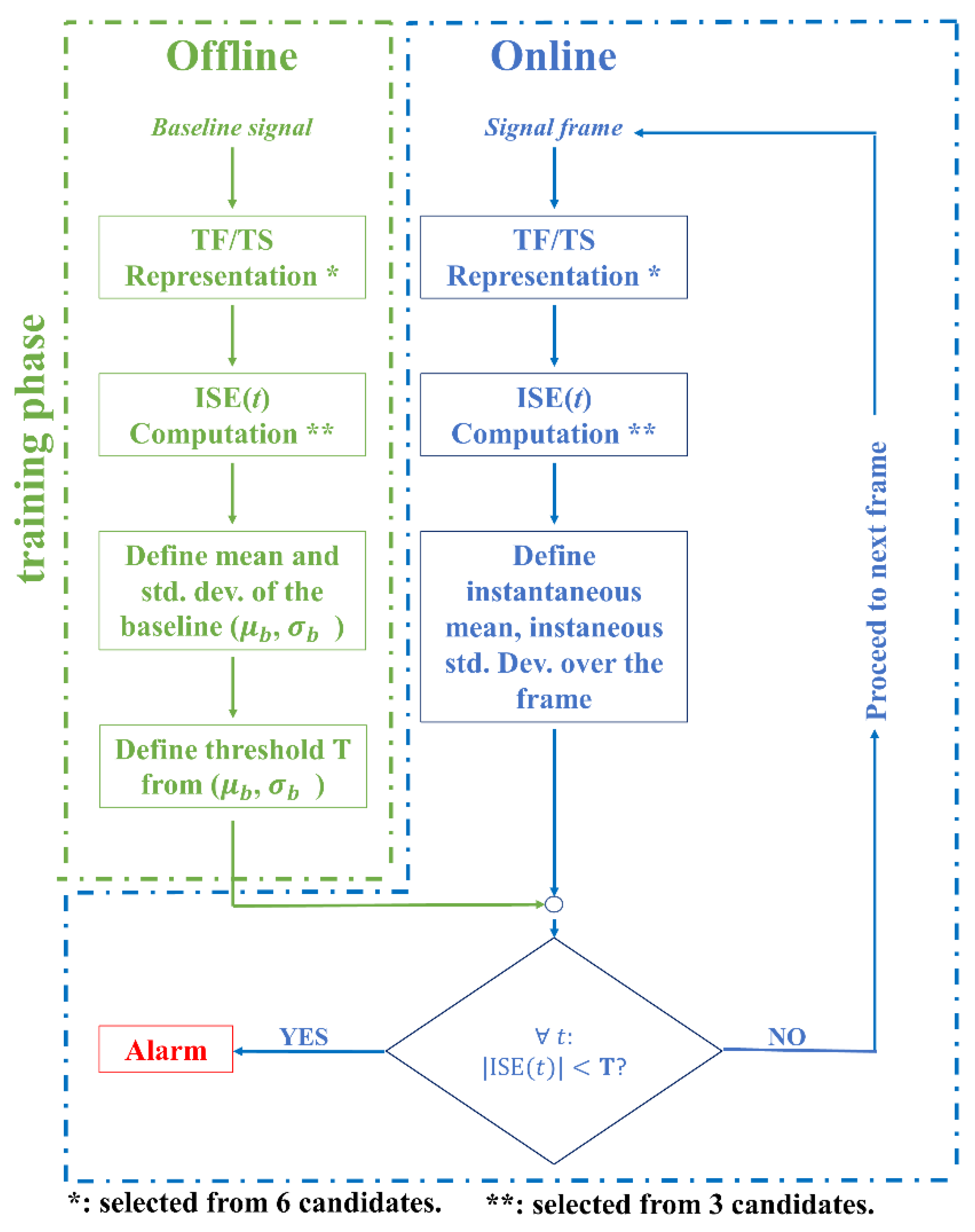
3. Methods: The Proposed Algorithm
As mentioned, the proposed algorithm is made up of three consecutive steps (portrayed in the flowchart of
Figure 1):
Time–frequency/time-scale transform of the recorded signal;
Computation of the instantaneous spectral entropy;
Comparison of the ISE time history with a baseline model.
In this sense, it can be seen as an application of the classic four-step statistical pattern recognition (SPR) paradigm proposed by Farrar et al. [
22], considering a small moving window of recent history over a continuous data stream. The specifics of this time-framing strategy will be detailed in the next subsection. Please note that, in the context of this research, the term ‘online’ refers to any part of the algorithm that is executed in real-time on the continuous stream of acquired data. The term ‘offline’ refers to any component of the algorithm that can be performed in advance and remains unchanged thereinafter (specifically, the training phase over the linear, undamaged baseline).
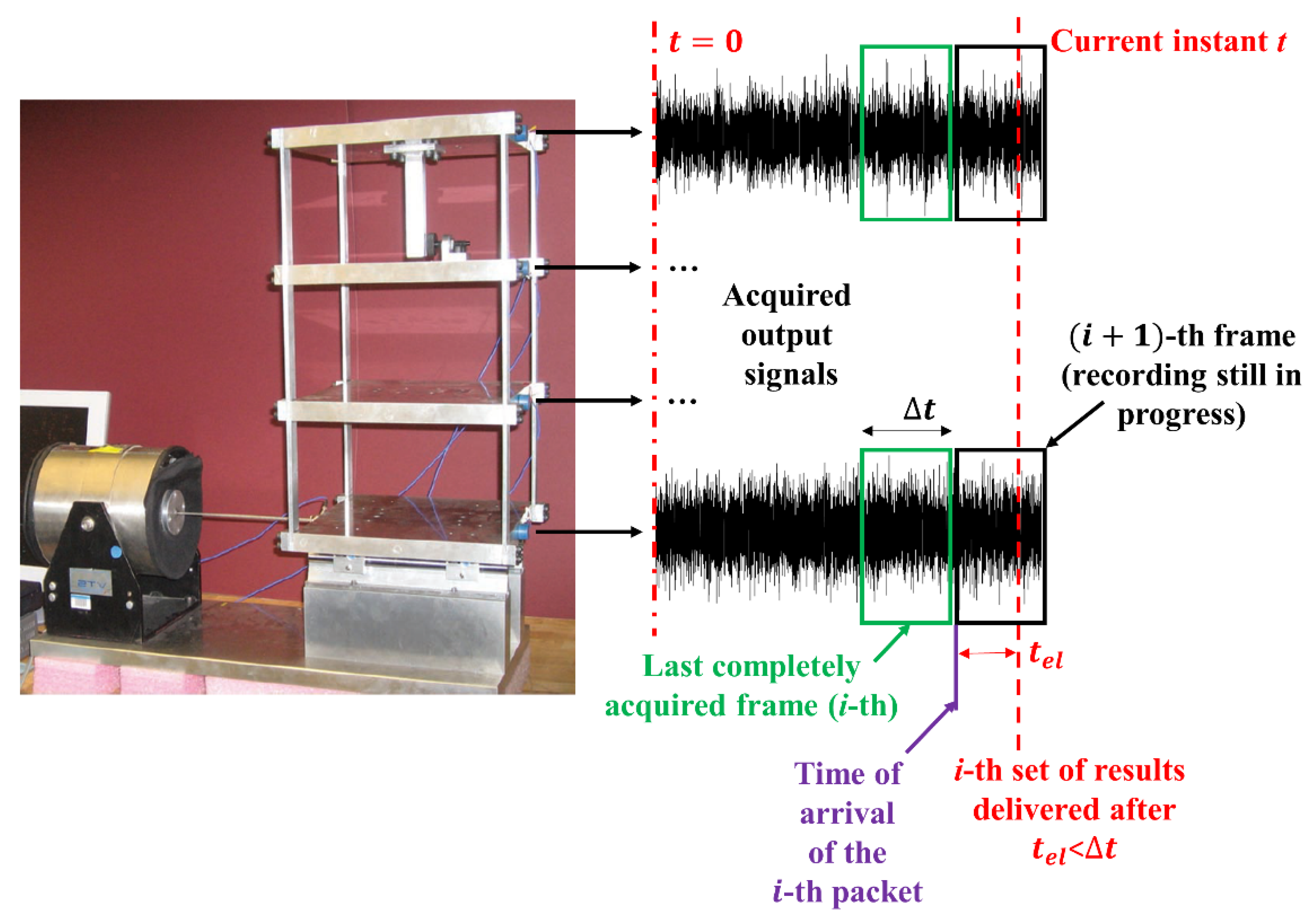
3.1. The Signal Framing Procedure
To have a continuous (uninterrupted) flow of results as the measurements keep on arriving in real-time, the input signals need to be segmented into short frames.
Indeed, signal framing is often encountered for signal processing techniques unable to deal with nonstationary signals (e.g., in cepstral analysis [
4,
23]). In this application, the framing is rather utilised to subdivide the continuous stream of data into discretised packets, as portrayed in
Figure 2.
The major practical limitation is that each data packet (received at the instant ) must have been fully processed before the arrival of the next one (delivered at ). Thus, being the time interval between subsequent arrivals, the elapsed time for the algorithm is required to be for any frame.
includes two main contributions, namely, the acquisition and transmission time. In turn, the latter contribution is made up of several procedures such as data uploading, downloading, and other intermediate steps. However, the end-to-end (one-way) delay can be realistically assumed as constant for all packets. Since the acquisition time is generally set as a constant as well, can be considered equal for any frame.
3.2. Candidate Entropy Definitions
In the next subsections, some theoretical recalls for the candidate TF/TS distributions and ISE definitions are provided. The aim is to optimise steps (1) and (2) of the proposed algorithm.
Only for completeness, the candidate definitions are reported firstly in their canonical (time-independent) formulation. Their extension for time dependency (i.e., their formulation for instantaneous values) is then discussed in the following subsection.
3.2.1. Shannon Spectral Entropy
The spectral entropy (SE) of a signal measures the uniformity of its spectral power distribution. When this is based on the Shannon entropy, this is also known as Shannon spectral entropy [
25]. In its original definition, provided by Claude E. Shannon as a measure of uncertainty in [
26], the SSE is defined over a probability distribution
as
for
frequency points (i.e., bins), where
is built from the (discretised) power spectrum
, and
is the discrete Fourier transform (DFT) of the whole signal. For this reason, the signal must be necessarily stationary (i.e., time-invariant).
The log function in Equation (1) can indiscriminately be the binary, natural, or base 10 logarithm (or any other base) depending on the intended notation and units of information considered, with no major conceptual differences. Here, the base 10 logarithm will be applied. The minus sign is only added to have a positive value, since
, and, therefore,
. The SSE with this classic definition has been applied by several authors to stationary signals for fault detection and diagnosis, e.g., in [
27].
It is worth noting that the same SSE can be estimated by substituting the power spectrum in Equation (2) with any form of TF/TS power distribution, i.e.,
. In this case, the probability distribution becomes
considering all of the timestamps between
and the signal total duration
. The spectral entropy will still return the same results as Equation (1); yet this allows, as will be specified in the following subsection, us to define the probability distribution at any time
. This will be essential for the definition of instantaneous SSE.
Please note that SSE can be normalised by simply dividing Equation (1) by , i.e., the maximal SSE obtainable (which corresponds to a WGN signal, uniformly distributed over the whole frequency range of interest). However, for the aims of this study, the standard (non-normalised) definition of spectral entropy has been applied. This has been preferred over the normalised variant to represent the differences in absolute terms produced by different time–frequency transforms. In fact, the normalised SSE is limited—by definition—to , whereas the SSE value in v can span from to . In the results of this research, it will be shown that the exact value depends significantly on the TF/TS distribution utilised.
3.2.2. Wiener Entropy
The Wiener entropy is another measure of the uniformity of the power spectrum. For this reason, it is also known as ‘spectral flatness’. Specifically, it is defined as
which corresponds to the ratio of the geometric and arithmetic mean of the signal in the frequency domain (
and
, respectively). Like all the other definitions of entropy, the WE does not have any measurement unit, i.e., it is a pure number. However, differently from the SSE, it ranges from 0 to +1. This derives from the inequality of arithmetic and geometric means, which states that (1) the geometric mean of a list of non-negative real numbers is always smaller than or equal to the arithmetic mean of the same list; (2) the two means are equal if and only if all the (real and non-negative) numbers in the list are equal, independently of their exact value. Therefore, +1 indicates a perfectly flat (uniform) frequency spectrum (as said, a WGN signal) and 0 means a pure tone. In between the two extreme values, the WE of a narrow power spectrum approaches zero, whereas a broader one has a larger value, getting closer to the unit value.
The advantages and limitations of WE in comparison to SSE have been analysed in detail by Ceravolo et al. [
10,
11]. As recalled in
Section 2, it emerged from these studies that the SSE is more stable and thus more suitable for inhomogeneous building materials, and thus for masonry and concrete structures, while less sensitive to structural changes (including damage). The WE, being more sensitive to both structural and non-structural changes, was contrariwise suggested for metallic structures, with more uniform construction materials and fewer nonuniformities [
12]. This allows us to take advantage of its major sensitivity with fewer false positives [
12,
13].
3.2.3. Rényi Entropy
The Rényi entropy can be defined, in its most generalised form, as
which indicates a family of generalised information measures rather than a single formulation [
28]. These are defined according to the arbitrary order
, where
and
. As in the previous cases, the base 10 logarithm is applied here, even if the base 2 and natural logarithm are also commonly utilised. It can be noticed that the Rényi entropy serves as a generalisation of the SSE since Equation (5) reduces to Equation (1) if
(as proven in [
29]). This limiting case can therefore be seen as
. Indeed, the general form of Equation (5) can also assume the specific forms of the Hartley or max-entropy (
), the min-entropy (
), and the collision entropy (
) as special cases. This latter case is the most common one and it is therefore generally simply known as ‘Rényi entropy’ for antonomasia. In this case, the particular formulation turns out to simply be
where
can be indistinctly defined as in Equations (2) or (3). The name ‘collision entropy’ derives from its main property. Given two discrete random variables
X and
X′, which are independent yet with an identical associated probability distribution (that is to say, i.i.d. variables),
indicates the probability of
X and
X’ colliding, i.e., casually yielding the same value, or
Equation (6) can thus be interpreted as .
This latter form, RE2, will be followed in this work. The rationale is that the collision entropy has been successfully proposed as an uncertainty quantifier [
30], i.e., as a measure of the Gaussianity of a random process. This has been employed in several signal processing fields, such as for biomedical engineering purposes [
31].
Similarly to the SSE, the RE2 values span , and will be reported here in this fashion, even if they can be easily normalised between .
3.3. Instantaneous SE
For real-time applications, all of the previously described entropy measures need to be adapted for instantaneous estimation.
By considering any TF/TS power distribution, similarly to Equation (3), one can define the probability distribution at time
as
which leads to the instantaneous estimate of SSE at time
, i.e.,
The same procedure applies to the instantaneous WE, leading to
and to the instantaneous RE2
Thus, for all definitions, the spectral densities must be computed through some sort of time–frequency representation of the signal. This is not a technically difficult task, and several options are available in this regard.
3.4. Candidate Time-Frequency Transforms
For the sake of this research, the six candidate TF/TS algorithms mentioned earlier (WV, DCW, STFT, and CWT with the Morse, Morlet, and bump mother wavelets) have been considered. In all cases, these will be presented here considering a discrete vibration signal (i.e., indistinctly a displacement, velocity, or acceleration time history), , where corresponds to for simplicity (by consequence, the total duration corresponds to the last timestamp ).
3.4.1. The Short-Time Fourier Transform
The STFT is the most classic approach for analysing the frequency content of a nonstationary signal over time. The basic concept is to divide the overall non-stationary signal into subsequent frames, which can be assumed to be internally stationary. The algorithm applies a standard DFT over a sliding window of fixed length
, which is moved over the original signal at fixed intervals of
samples. The values of
and
are arbitrarily set, according to the intent and specific case, and result in an overlap
among neighbouring windowed segments (that is to say,
). The resulting number of DFTs is equal to
where the writing
indicates the floor function (to round up non-integer divisions). The outcome of this TF analysis is a matrix of ordered DSFs, i.e.,
Of course, Equation (13) represents the discretised form of . In the specific case of the SFTF, its squared magnitude is also known as the spectrogram of the signal .
The generic
-th element in Equation (13) can be computed as
i.e., the DFT of the data window centred around the timestamp
. The term
indicates a generic function for windowing. The choice of the specific windowing function is arbitrary; however, in general, any
has some sort of ‘tapering off’ at both edges to avoid spectral ringing artefacts. For the sake of this study, the STFT was computed over the Nyquist range
. The data were windowed with a Hann window of length 8 with six samples of overlap between adjoining segments and a 128-point FFT.
It is important, before proceeding, to recall that the STFT has several advantages but also limitations. As an operator, it is linear and invertible; it is also relatively easy to compute. However, it is not positive-defined, and the several classic issues due to the applications of the DFT to a finite time window (which does not start at and ends well before ) are further exacerbated by the short duration of each frame. That is to say, the frequency resolution of the STFT depends on the window width, and it decreases when the time resolution increases. The STFT does not provide the ability to localise transients to the width of the window and thus does not have the same degree of accuracy as, e.g., the CWT, which will be discussed later.
3.4.2. The Wigner–Ville distribution
The WV distribution was defined in the first applications of Wigner in quantum theory [
32] and the following works of Ville in signal theory [
33]. The Wigner–Ville spectrum then gained popularity as a generalised spectrum for time-varying spectral analysis [
34]. This can be defined as the Fourier transform of the instantaneous autocorrelation function (ACF), or
. This latter operator can be written, in its discretised form, as
which is a time-dependent correlation measure between the time series
and its complex conjugate
; then, one has
where the summation is carried out on the variable
, i.e., the time lag for the estimate of the autocorrelation sequence, for each discrete timestamp. For this application, the number of time lags considered to estimate the instantaneous ACF was set as equal to half of the signal length (that is to say, being the signal divided in subsequent frames, to half of each frame length).
A technical issue is that, for any odd value of , Equation (16) requires evaluating the signal at half-integer sample values. In order to be performed, this requires interpolation between the discrete timestamps. In turn, to avoid aliasing problems, this requires zero-padding the DFT.
Even more importantly, due to its quadratic nature, the WV transform suffers from the emergence of interference terms. That is to say, in a multi-component signal, the mixing of each pair of frequencies (
,
) will produce these spurious terms, which will be located at the average frequency
and oscillate at the difference between the two frequencies. This issue can be partially attenuated with the smoothed pseudo-Wigner–Ville (SPWV) distribution, where independent lowpass windows are used to smooth in time and frequency. This approach has proven to be viable for the condition monitoring of rotating machinery, with a significant reduction in the presence of spurious cross-terms [
35]. Another option to overcome these problems, quite closely related to SPWV [
36], is the discrete Choi–Williams distribution.
3.4.3. The Discrete Choi–Williams Distribution
The DCW [
37] departs from what is defined in Equation (16) and further considers a two-dimensional filtering step in the so-called ambiguity domain to remove the interference terms. In this sense, it applies an ambiguity function (AF), which serves as a transformation from the ACF domain to the AF domain. This ambiguity distribution can be seen as the STFT of the signal
using the signal itself as the windowing function [
38]. In the AF domain, the interference terms have specific properties and are located at specific locations, far from the autoterms of interest. This way, the spurious components can be easily distinguished, and thus effectively attenuated by multiplying with a kernel function directly defined in the AF domain. Specifically, the DCW utilises the exponential kernel known as the Choi–Williams kernel function. Its definition is the following:
where
is the time lag, already seen in the definition of the WV distribution,
is the doppler shift, and
is the so-called selectivity parameter, which should be greater than zero and is (generally)
for many applications, even if it can potentially assume much larger values.
Thanks to the specific shape of the 2-D filter defined in Equation (17), the cross-terms that are located far from the origin and axes of the AF domain (i.e., that have a significant time delay and frequency shift) are thus filtered out. That is to say, this suppresses the interferences that result from the components that differ in both the time and frequency centre. The filtered signal is then transformed from the AF to the TF domain, where it can be finally used. Of course, considering different kernel functions will return different properties for the final outcome in the time–frequency domain.
For the reasons described above, the DCW depends largely on its parameters, especially for the definition of the (discrete) ambiguity function. For this research, a selectivity parameter equal to 0.5 was considered. The same as applied for WV was utilised for DCW as well.
This concludes the first set of candidates. They are all defined in the TF domain. Strictly related to them, the second set of three more candidates is composed of the continuous wavelet transforms with different mother wavelets.
3.5. Candidate Time-Scale Transforms
Wavelet-based approaches have been applied extensively for SHM problems (see, e.g., [
39]), thanks to their several advantages. The complete theory about wavelets is too long to be recalled here; one can find the necessary background in the works of e.g., Daubechies [
40] and Rioul and Vetterli [
41]. Many other comprehensive works can be found in the literature or dedicated textbooks, e.g., [
42].
As their main feature, wavelets can be depicted as brief oscillations, i.e., time-limited (as in this application here) or space-localised small wave-like functions. This is profoundly different from harmonic functions, such as sines and cosines, which span unaltered from
to
and thus do not allow for time resolution. For this and other reasons, the (discrete or continuous) wavelet transform is known to be more able to adapt to random and/or nonstationary signals than Fourier transform [
43]. In turn, this can be used, e.g., to depurate the signal of measurement noise or to separately investigate the underlying linear and/or stationary components (by discarding the nonlinear/nonstationary components). For instance, it was demonstrated experimentally in [
44] how the CWT-extracted entropy can be used to detect small damages (e.g., a 5% reduction on bolt-tightening torques).
A major aspect is that, differently from sinusoids, a unique definition of a wavelet does not exist. Indeed, DWT or CWT can use a variety of different basis functions, also known as mother wavelets. Any zero-mean function that satisfies some basic conditions, such as regularity and admissibility [
45], can be used as a mother wavelet.
The arbitrariness in the definition of the mother wavelet allows for the tailoring of the TS analysis for the specific signal of interest. Here, three different options have been tested: the bump, Morse, and (analytical) Morlet wavelets. All of these candidates are based on functions
that rapidly decrease in time. These three options have all the advantages of being analytic; that is to say, they are complex-valued and their Fourier transforms are supported only on the positive real axis of the frequency domain. Since these complex wavelets respond solely to the non-negative frequencies for any given signal, their transform will have a less oscillatory modulus than in the case of a real-valued wavelet [
46].
This advantageous property enables better detecting and tracking capabilities for instantaneous signal parameters.
The basic characteristics of these three candidates will be briefly recalled here for completeness’ sake. In all cases, the continuous wavelet transform of the signal
can be expressed (in its continuous form) as
i.e., as a product in the frequency domain, where
is the complex conjugate of the Fourier transform of the child wavelet. This is a scaled and time-shifted version of the original mother wavelet, defined by the scale parameter
and the (time) shift parameter
as
The resulting time-scale representation can then be utilised to estimate the instantaneous spectral entropy of the signal, exactly as carried out for the time–frequency transforms encountered previously.
3.5.1. The Morse Wavelet
The definition of the Morse wavelet derives mostly from the works of Olhelde and Walden [
47] and Lilly and Olhelde [
48]. In their generalised form, this family of mother wavelets can be defined according to the two parameters
and
as
where
characterises the symmetry of the Morse wavelet and
is a compactness parameter defined as
. In turn,
is known as the time-bandwidth product. The other two terms,
and
, represent (in the same order) the Heaviside (or unit) step function and a normalizing constant.
The parametrization of the generalised Morse wavelet (described in detail in [
49]) allows us to define several other analytical wavelets as special cases. For instance,
will return the Cauchy family of wavelets. For the sake of this research,
and
were considered. A detailed analysis of the influence of the GMW parameters for ISE estimates can be found in [
20].
3.5.2. The Analytic Morlet Wavelet
The analytic Morlet wavelet is a complex sinusoid modulated by a Gaussian envelope, i.e.,
and thus its Fourier transform becomes
where
is needed to enforce the unit energy requirement for the wavelet and
is the central frequency of the wavelet (in radians). This determines the number of oscillations of the complex sinusoid inside the Gaussian envelope; to ensure that Equation (21) has zero mean, as required for any wavelet,
must be greater than 5, which can be a limitation on some applications. For the sake of this research,
was used.
3.5.3. The Bump Wavelet
The last candidate, the bump wavelet, differs from the analytical Morlet wavelet since it has an unequal spread. Specifically, it has a wider variance in time and is narrower in frequency. The Fourier transform of its mother wavelet can be defined as
where
indicates the indicator function, here applied in the frequency interval
.
and
are customisable parameters that regulate the frequency and time resolutions. Here, these were set to 5 and 0.6, respectively.
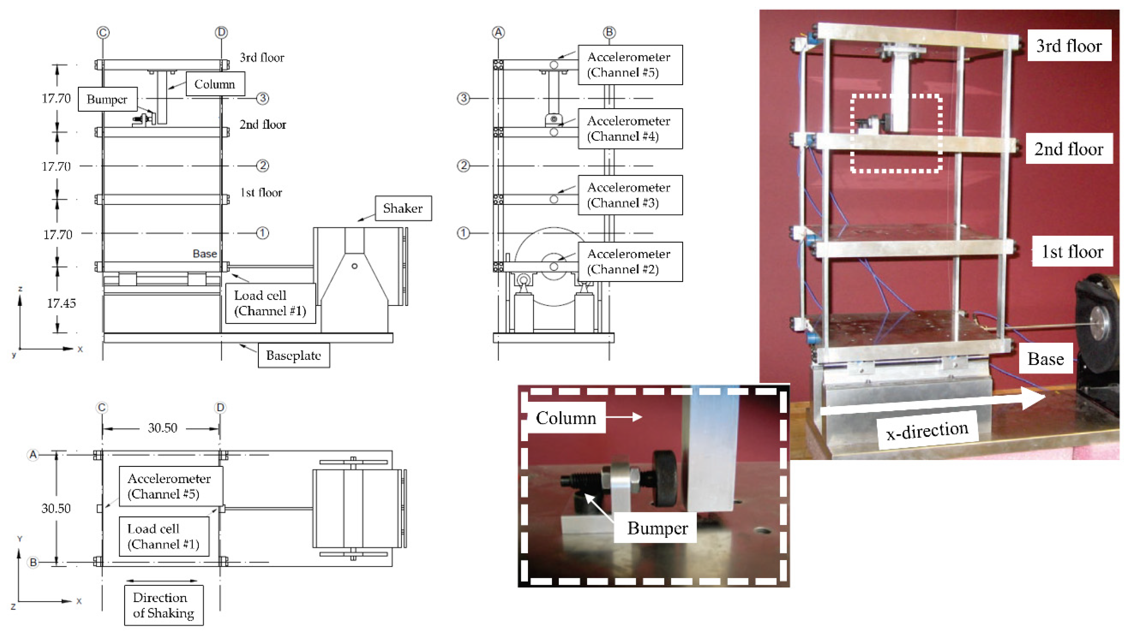
4. Materials: The Experimental Case Study
The experimental dataset utilised for this investigation originates from the well-known frame structure built at the Engineering Institute (EI) of the Los Alamos National Laboratories (LANL), depicted in
Figure 3. This case study is widely used by the SHM community as a benchmark problem for linear and nonlinear damage scenarios.
4.1. The Multi-Storey Frame Structure
The three-storey structure serves as a scaled-down mock-up of a typical metal structure. It is made up of an aluminium baseplate (76.2 × 30.5 × 2.5 cm) and four aluminium plates (30.5 × 30.5 × 2.5 cm), connected at each floor by four aluminium columns (17.7 × 2.5 × 0.6 cm). It was excited by a WGN driving force, defined between 20–150 Hz and applied at the base, which rested on rails [
24].
For the intended purpose, the use of random noise in input is suitable for an entropy-based approach; indeed, the input as intended by the authors of the original dataset can be seen as a good approximation of the frequency content of AVs, even if their actual amplitude is generally in the order of magnitude of .
The structural response was recorded at four output channels, one per floor (including the base). These were purposely mounted at the centre line of each floor to measure the system’s response along the x-direction while being insensitive to the flexural modes along the y axis, as well as the torsional ones [
24]. A sampling frequency
Hz and a total duration of
s were set, resulting in 8192 data points per acquisition. More technical details about the structure and the acquisition procedure can be found in [
24].
17 different structural configurations (enlisted in
Table 1) were inspected. Fifty acquisitions (hereinafter referred to as ‘instances’) per state were performed. State #1 served as the (linear) baseline for the pristine structure with no mass nor stiffness alterations.
Two models of damage were considered:
These two damage typologies are representative of the classic ‘fully open’ [
51,
52] and ‘breathing’ [
50,
53] crack models.
In the first case, the stiffness change was induced by replacing the corresponding column with another one, built from the same materials and with the same geometry, except for the cross-section thickness, which was halved in the direction of shaking.
In the second case, the source of nonlinearity (specifically, an additional bilinear stiffness) was mimicked by a one-sided constrain, mounted between the second and third floors of the frame (see the zoom box in
Figure 3). This mechanism worked as follows: the column (suspended from the lower side of the top floor) impacted with the bumper (attached on the upper side of the bottom floor) when oscillating in the negative x-direction, with an increase in stiffness with respect to the free oscillations along the positive x-direction. Thus, it acted as a pointwise source of bilinearity, similarly to the breathing crack (where, instead, the stiffness is reduced while oscillating in the direction where the crack opens), even if, in this case, the overall equivalent stiffness increased rather than decreased [
54]. Nevertheless, it similarly added harmonic distortions in the structural response due to the occurrence of sub- and super-resonance vibrations [
55]. The amount of this distortion was adjusted by moving the bumper further or closer to the column.
Configurations with additional masses were considered as well in order to mimic changing operating conditions; it must be said, however, that abrupt variations in structural mass can be ascribed to damage occurrence as well, e.g., during seismic events.
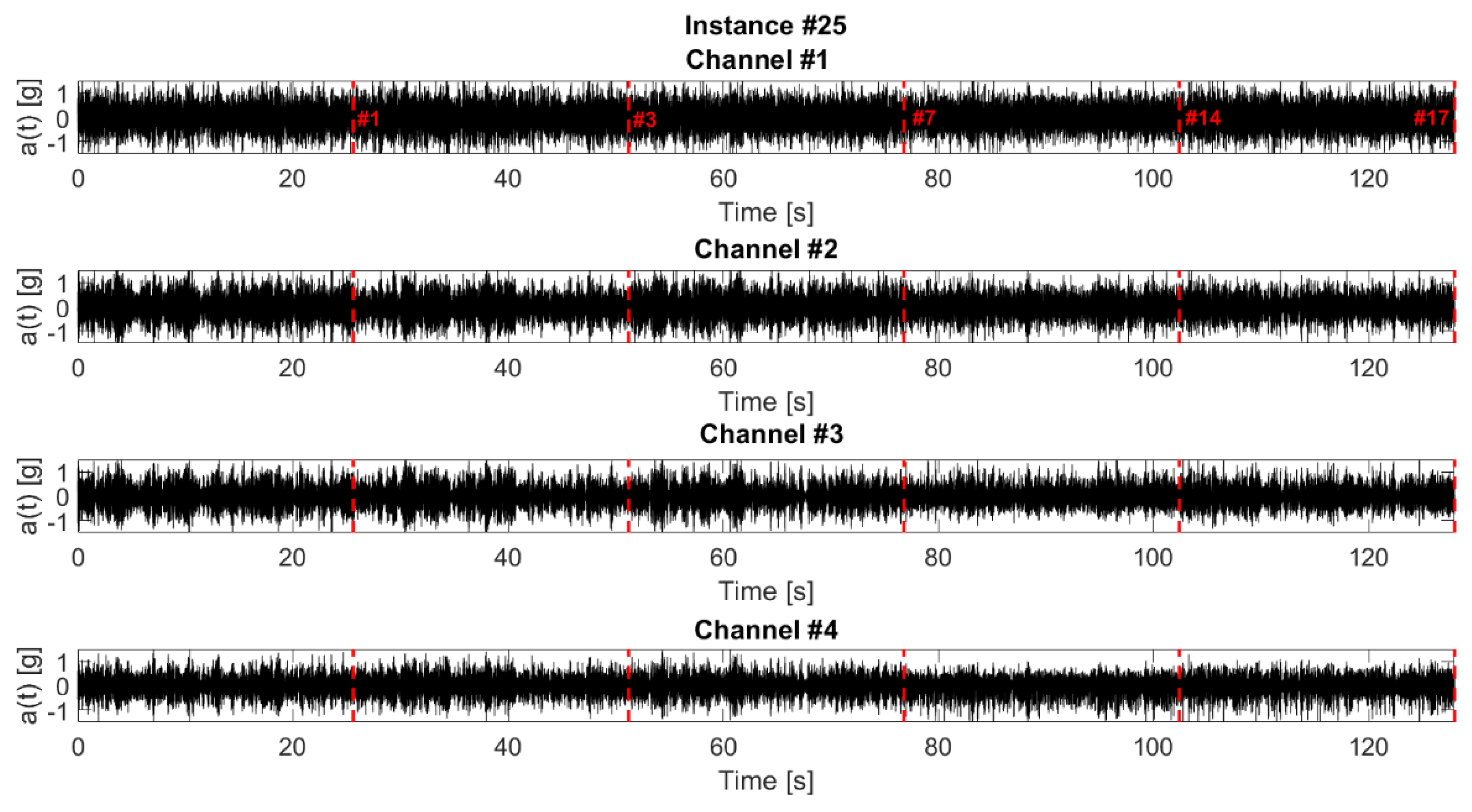
4.2. The Concatenated Signal
By following the procedure described in [
24] (
Section 4.1), the signals from states #1, #3, #7, #14, and #17 were concatenated (
Figure 4) to emulate damage-unrelated structural changes, such as time-varying operational conditions (with additional mass overloads), or the instantaneous occurrence of damage. This operation was performed on the signals from all output channels and for all instances. The differences between the results from different sensor locations will be discussed in a dedicated subsection. No relevant variations were noticed for the 50 signals. Therefore, for illustrative purposes only, the 25th instance will be shown in all figures. To emulate real-time acquisition, the concatenated signals were framed into blocks of 6.4 s (corresponding to 2048 timesteps for the given sampling frequency), following the framing strategy described previously.
4.3. The Normality Model
Following the pattern recognition framework proposed by Farrar et al. [
22] for SHM, the damage-sensitive feature estimated from the baseline condition (state #1) can be used to train a normal operating conditions (NOCs) model. This is a classic approach similar to, e.g., what was carried out in [
54]. In this specific case, a Gaussian process regression (GPR, [
56]) was performed over the 2048 pairs of training data (ISE(
),
t) extracted from state #1. The threshold was defined as two times the standard deviation from the GPR-derived mean (i.e., a 95.45% prediction interval), i.e.,
.
Due to the stationarity of both the structural parameters and the external driving force, the ISE remains almost unchanged for the whole duration of the training dataset, thus returning an almost constant (time-independent) threshold for the baseline structural conditions, i.e., , .
It must be said that, depending on the size of the training dataset, the GPR might be computationally burdensome. For this application, when trained on the dataset as described above, it took, on average, 20.22 s. However, as mentioned previously, this step can be pre-emptively performed offline. Furthermore, for stationary NOCs, as in this case, the problem can be simply reduced to the estimate of the (time-independent) mean and standard deviation. The data-driven thresholds do not need further online adjustments unless the NOCs are purposely changed by the operator.
5. Results
To detail the advantages and limitations of each candidate, several factors must be considered and weighted. For this reason, this section will be organised as follows. Firstly, the effects of sensor placement are addressed. Then, the three candidate mother wavelets are compared with each other. The other three candidate algorithms for TF analysis are benchmarked as well in
Section 5.3. An overall comparison of TF vs. TS follows. Their sensitivity to the deleterious effects of framing is described in
Section 5.5. Next, the sensitivity to damage of the three candidate entropy definitions is discussed. Finally, being the computational time crucial for online monitoring, the computational efficiency of each alternative is assessed.
5.1. Effects of Sensor Placement
The third output channel, located on the second floor, always returned the data most responsive to structural changes for all candidate entropy definitions and TF/TS transforms. This can be explained by the specific damage scenarios analysed here, since the stiffness reduction in state #7 was located at the second interstorey, between the first and second floor, whereas the nonlinear mechanism (states #14 and #17) was attached between the second and third floor.
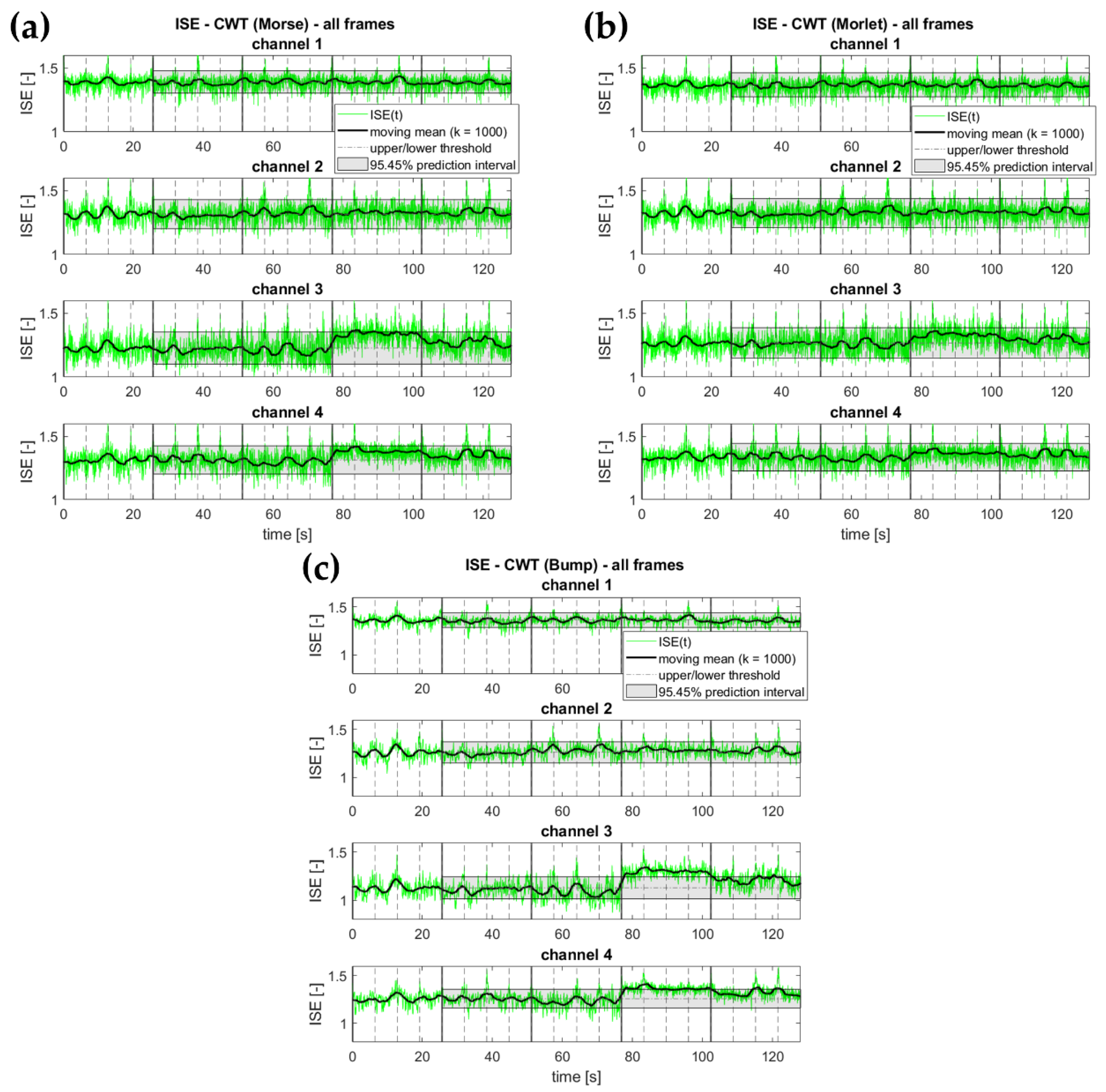
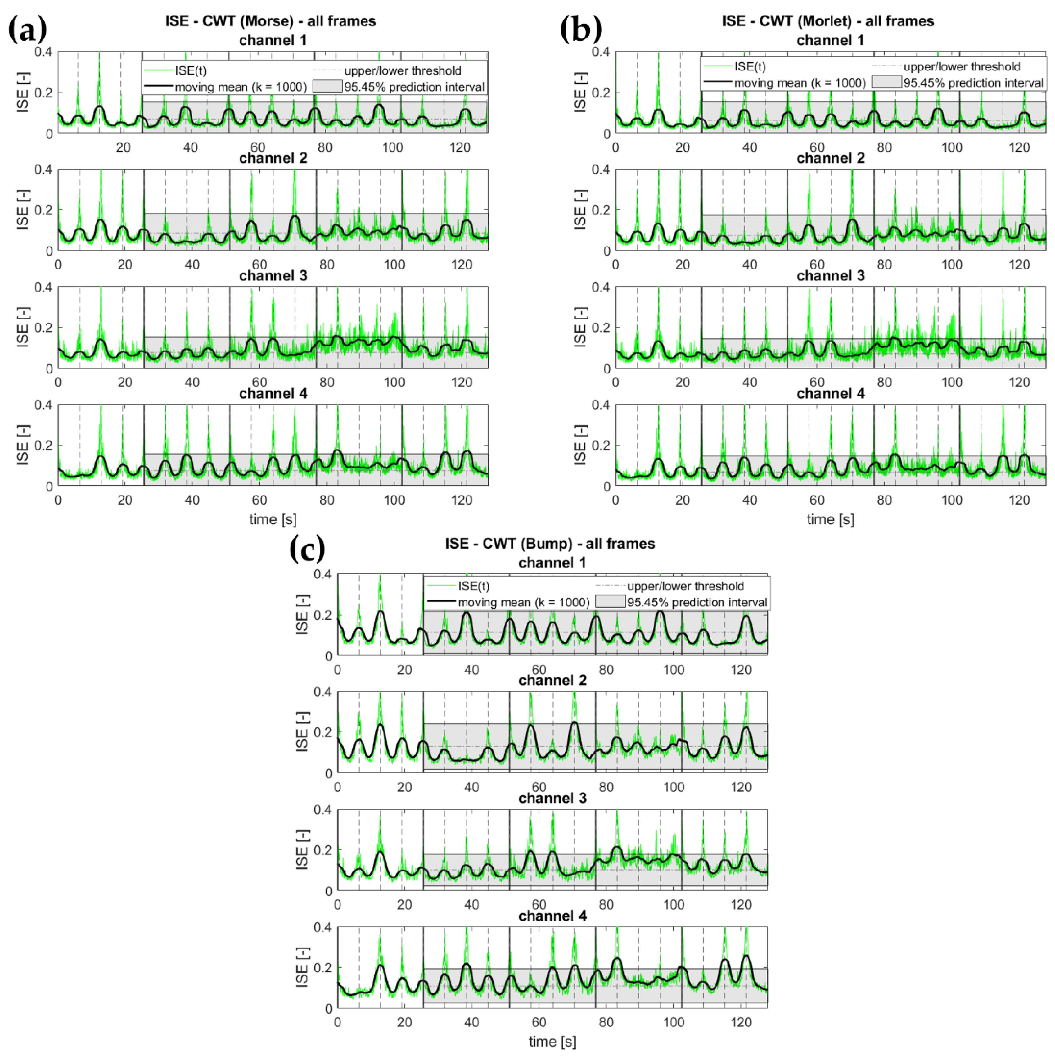
5.2. Effects of the Mother Wavelet Selection for TS Analysis
The results for SSE, WE, and RE2 considering the candidate TS representations are reported in
Figure 5,
Figure 6 and
Figure 7 in the same order. In all plots, the solid vertical lines indicate the end of the concatenated signals (states #1, #3, #7, #14, and #17), and the dashed ones at the end of the single frames (four for each state). The grey area in states #3 to #17 represent the 95.45% confidence interval defined from the GPR performed on the pristine baseline (state #1), which, as mentioned, is basically a constant value along time. The thin green lines represent the instantaneous spectral entropy, whereas the thick black ones the moving average of the same (computer over
timesteps). This latter addition was included to avoid the instantaneous trespassing of the threshold, which would have been physically meaningless. In fact, while sensitive to damage (as will be shown), the ISE was found to be highly affected by rapid fluctuations.
Among the three options considered here, the bump wavelet was the one with the best performance. This finding was confirmed for all of the definitions of entropy (RE2, SSE, WE).
The analytic Morlet wavelet was less sensitive to damage in all cases. Therefore, these preliminary results seem to indicate that an unequal TF variance (narrower in frequency, wider in time) is more sensitive to the occurrence of damage-induced nonlinearities.
The generalised Morse wavelet was not very responsive to either linear or nonlinear damage as well, at least for the parameters set here; a larger sensitivity analysis on the two parameters
and
can be found in [
20].
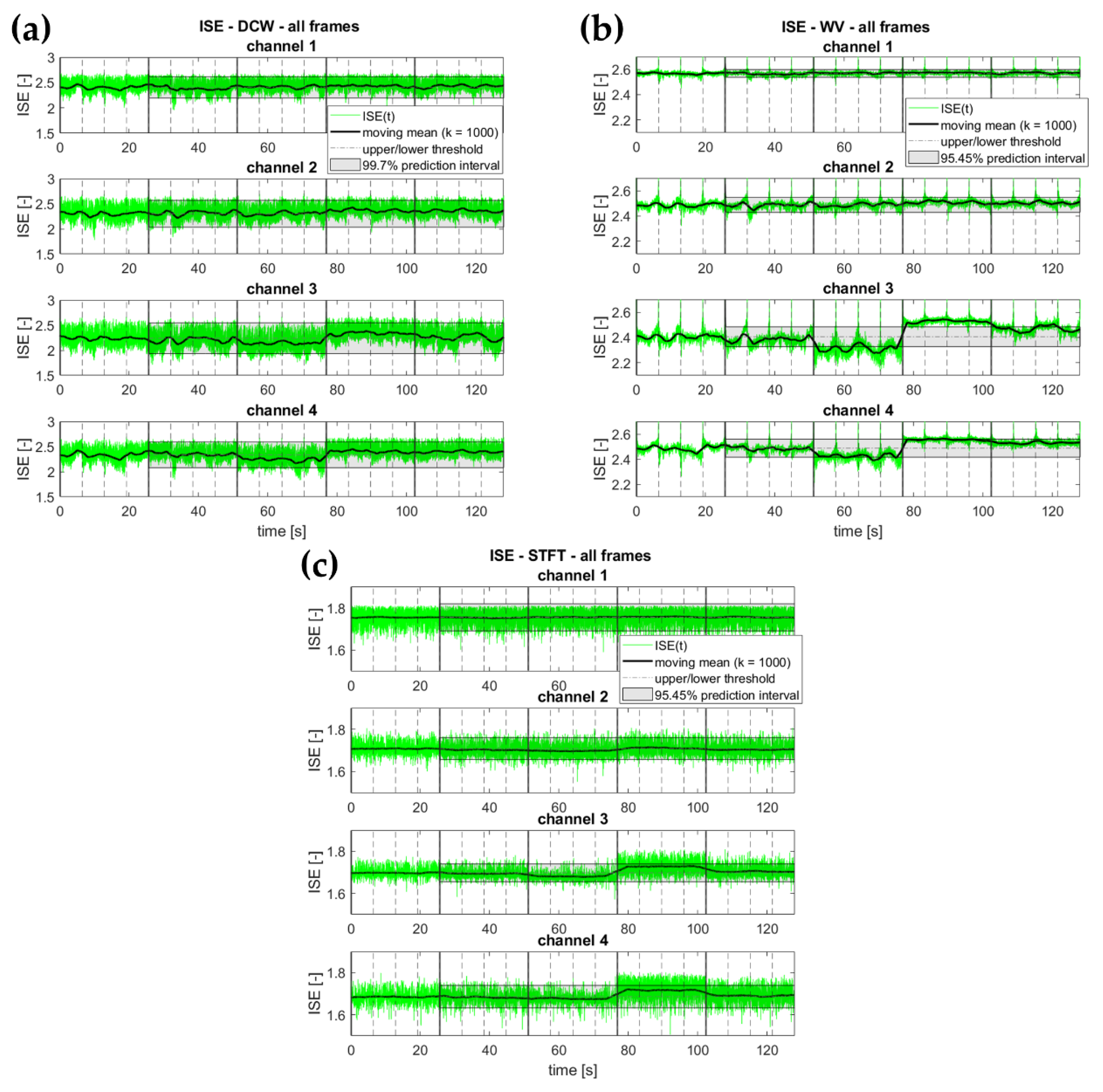
5.3. Effects of the Algorithm Selection for TF Analysis
The results considering the candidate TF representations are reported in
Figure 8,
Figure 9 and
Figure 10 (for SSE, WE, and RE2, in this order). The same indications provided before for
Figure 5,
Figure 6 and
Figure 7 apply to all of the plots in this second set of results.
For RE2 and SSE, the STFT returned the less useful results. For WE, the DCW was the less suited alternative. In all cases, the WV was the TF representation most sensitive to the occurrence of a structural nonlinearity. The sensitivity to the stiffness reduction in case #7 was more limited; however, it was still correctly detected under the statistically defined threshold with both RE2 and SSE.
It seems, therefore, that the ameliorations included in the DCW algorithm to overcome the WV technical limitations did not produce any increased damage detection capability.
5.4. Comparison of TS and TF
According to all of the results shown in
Figure 5,
Figure 6,
Figure 7,
Figure 8,
Figure 9 and
Figure 10, it can be said that—regardless of the specific algorithm (for TF analysis) or mother wavelet (for TS) considered—the time–frequency representations were returned as slightly more stable (i.e., less subject to fluctuations) and thus more useful estimations for ISE.
It is worth noting that ISE measurements extracted from WV, DCW, or STFT were noticeably less affected by distortions induced from the framing of the signal as well. This point will be discussed in further detail in the next subsection.
5.5. Effects of Framing
The framing of the signal in very short tracts generated undesired and deleterious edge effects, i.e., more or less pronounced deviations from the expected behaviour at both ends of any signal frame. For pattern-recognition-based SHM, this issue can be inconvenient due to the periodic, instantaneous trespassing of the data-driven threshold. As mentioned before, this problem was partially solved considering the moving mean of the ISE signal, defined for this specific case study over 1000 timesteps (~3.125 s).
These deleterious effects were particularly evident for the CWT, independently on the specific mother wavelet. This can be seen in the results reported in
Figure 5,
Figure 6 and
Figure 7. By way of illustration,
Figure 11 shows the cone of influence for one frame of the analysed signal. Edge effects may appear in the shaded region as signal artefacts due to stretched wavelets extending beyond the edges of the observation interval. Only the unshaded region can provide an accurate time-scale representation of the data.
These edge effects altered the data to such an extent that the results from the Wiener entropy/CWT combination were unusable. Even in the case of RE2 and SSE, these artefacts, while less severe, had a noticeable negative effect on CWT results. This difference derives from the definition of entropy applied: the WE, being the most sensitive to any variation in the signal (not only to damage), was more affected. The edge effects issue, while still visible, was less pronounced for VW, DCW, and STFT, with fewer consequences in terms of the stability of the results.
5.6. Sensibility to Damage and Structural Changes
As enlisted before in
Table 1, the different state analysed here includes
The occurrence of linear damage as a stiffness reduction;
The occurrence of nonlinear damage as a breathing crack mechanism;
The occurrence of damage-unrelated structural changes (i.e., added masses) to both the linearly and nonlinearly behaving structure.
The results must be interpreted according to the sensitivity of the instantaneous formulations of RE2, SSE, and WE to these different forms of ‘anomaly’. Specifically, all of the tested combinations were more sensitive to the nonlinearity introduced in state #14 (which is more nonlinear than case #17, due to the reduced gap between the bumper and the column). This reflects the larger variations in the frequency distribution of the signal power induced by the nonlinear mechanism.
As already mentioned, the WE was the most prone to framing issues. This can be explained by its known major sensitivity, which leads to disruptive consequences if combined with unphysical edge effects. Apart from that, RE2 and SSE returned quite consistent results, with no particularly relevant differences. This can be explained by SSE being a special case of generalised Rényi entropy, and thus not too dissimilar from the collision entropy considered for RE2.
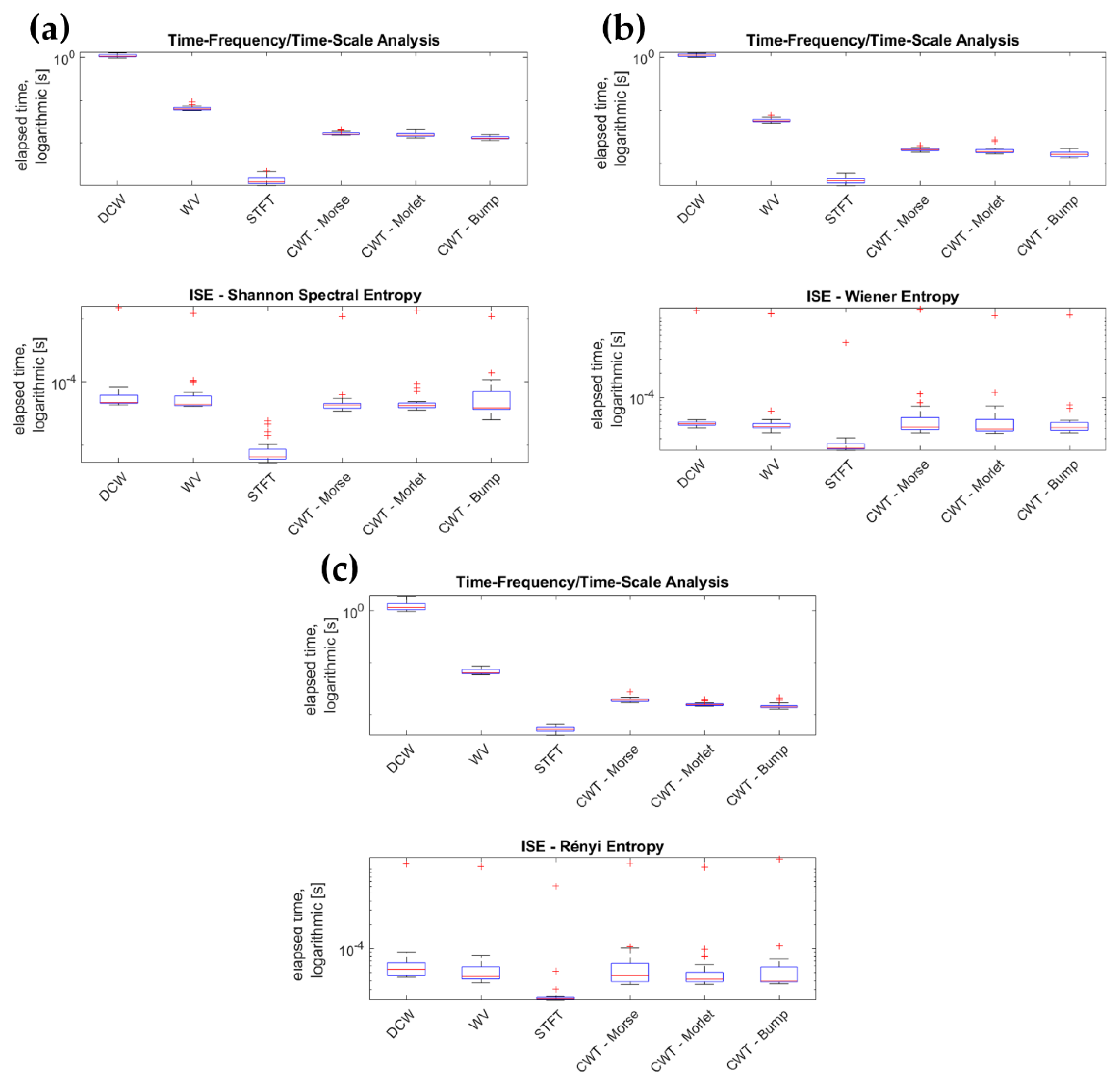
5.7. Computational Requirements and Feasibility for Real-Time SHM
All computations were run on a laptop equipped with Windows 10.64-bit, Intel Core i7-7700HQ with CPU 2.80 GHz and 16.0 GB RAM, and MatLab R2020b.
The total duration (comprehensive of TF/TS analysis and ISE calculation) is reported in
Table 2 for the six candidate algorithms. The reported values correspond to the average time (calculated over all frames of the whole concatenated signal). As can be seen, the elapsed time was well below the frame duration (6.4 s) for all combinations. This makes all of them potentially eligible for online application, by a large margin.
Figure 12 shows the boxplot diagrams for all combinations, considering separately the TF/TS representation and the ISE calculation from it. As it can be seen, the TF/TS transform was the ‘bottleneck’ of the whole procedure, independently of the specific entropy definition applied. The actual calculation of the ISE did not significantly slow down the execution, being one to two orders of magnitude faster. Please notice that the time axis is reported on a logarithmic scale in
Figure 12. Indeed, the DCW performed significantly slower than the other approaches. Consider also that the STFT is only apparently much faster than the other approaches due to the fewer calculations performed. All of the other algorithms were set to return consistent TF/TS representations, i.e., an
-by-
matrix, where
is the number of frequency samples (for DCW and WV) or scales (for CWT), and
is the number of time samples in the provided time history. For the chosen frame duration and considering only frequencies up to
(80 Hz) to avoid any alias issue, this corresponds to 40,960 elements in the
matrix. On the other hand, with the settings described in
Section 3, the STFT returned 20-by-1021 elements (totalling 20,420). Nevertheless, further increasing the resolution in both the time and/or frequency domain did not noticeably improve the effectiveness of the STFT results, which remained poor overall, as previously mentioned.
5.8. Discussion
The results presented in this section can be summarised as follows:
The best mother wavelet candidate is the bump wavelet;
However, TF analyses generally returned more stable results than TS procedures. They were also (much) less affected by edge effects;
Among the three TF candidates, the Wigner–Ville distribution was the most sensitive to both linear and nonlinear damage. The STFT was outperformed by any other available option;
Differently from what was expected, the DCW algorithm did not perform better than the classic WV. However, the properties of the DCW depend largely on its sensitivity parameter . Further studies will be needed to assess the potential of DCW with different values, and to test other ambiguity function approaches for TF;
The best overall results were achieved at the third-floor channel with WV paired with SSE. The WV/RE2 combination showed good damage sensitivity as well;
All algorithms were validated as computationally efficient and suitable for quasi-real-time applications (by resorting to a framing strategy, such as the one described here).
6. Conclusions
This study investigated the feasibility of instantaneous spectral entropy (ISE) as a time-dependent damage index for online SHM. The proposed feature has the advantage of being suited to nonlinearly behaving structures and nonstationary signals. Two main steps are required for the implementation of the proposed ISE approach: (1) the time–frequency/time-scale analysis of the recorded output signal, and (2) the estimation of the instantaneous entropy from it.
Six candidate algorithms have been tested for step (1)—namely, the discrete Choi–Williams, Wigner–Ville, and short-time Fourier transforms, plus the continuous wavelet transform with Morse, Morlet, and bump wavelets. These have been combined with three entropy definitions, applied in step (2)—the Shannon spectral, Wiener, and Rényi (with ) entropies.
All of these combinations were investigated on an experimental benchmark dataset: a three-storey frame structure from Los Alamos National Laboratories. This case study was selected as its data include linear and nonlinear structural conditions and can be used to mimic a nonstationary system. The candidates’ performances have been analysed in terms of their sensibility to sensor placement, computational efficiency (i.e., elapsed time), the influence of framing, and responsivity to damage-related and -unrelated structural changes (both linear and nonlinear). In general, all of the combinations investigated here seemed to be more sensitive to the inclusion of a nonlinear source rather than a decrease in stiffness. Therefore, the proposed approach is specifically suggested for breathing cracks or similar damages.
For real-time damage detection, the computational efficiency requires a trade-off between the accuracy and the rapidity of the TF/TS analysis, which is the bottleneck step in the procedure. All of the six alternative TF/TS representations were found to be suitable in this sense, with only the DCW being relatively slower but still potentially applicable. On the other hand, the computational time for the ISE computation is negligible in comparison.
Since the computational effort of any time–frequency transform increases with the signal duration, it has been proposed here to segment the continuous datastream into 6.4 s-long blocks. The whole procedure runs in less than 1 or 2 s; therefore, the algorithm can operate seamlessly without interruptions. That is to say, the results of the previous frame are delivered before the end of the one currently on record.
For this specific case study, the most promising results were found with the Shannon spectral and Rényi entropies when applied to the Wigner–Ville distribution. The findings of this research will serve for future applications of instantaneous entropy measurements to SHM problems for civil engineering purposes, including in situ tests on real-scale buildings, as well as in related fields, such as the structural analysis of aerospace and mechanical systems.
Author Contributions
Conceptualization, M.C. and C.S.; methodology, M.C. and C.S.; software, M.C.; validation, M.C.; formal analysis, M.C.; investigation, M.C.; resources, C.S.; data curation, M.C.; writing—original draft preparation, M.C.; writing—review and editing, C.S.; visualization, M.C.; supervision, C.S.; project administration, C.S. All authors have read and agreed to the published version of the manuscript.
Funding
This research received no external funding.
Institutional Review Board Statement
Not applicable.
Informed Consent Statement
Not applicable.
Data Availability Statement
All the data used in this article have been made available upon request by the Los Alamos National Laboratory.
Conflicts of Interest
The authors declare no conflict of interest.
References
- Farrar, C.R.; Worden, K. Structural Health Monitoring: A Machine Learning Perspective; John Wiley & Sons, Ltd.: Hoboken, NJ, USA, 2013. [Google Scholar]
- Carden, E.P.; Brownjohn, J.M.W. ARMA modelled time-series classification for structural health monitoring of civil infrastructure. Mech. Syst. Signal Process. 2008, 22, 295–314. [Google Scholar] [CrossRef] [Green Version]
- Civera, M.; Zanotti Fragonara, L.; Surace, C. A novel approach to damage localisation based on bispectral analysis and neural network. Smart Struct. Syst. 2017, 20, 669–682. [Google Scholar]
- Ferraris, M.; Civera, M.; Ceravolo, R.; Surace, C.; Betti, R. Using Enhanced Cepstral Analysis for Structural Health Monitoring; Springer: Singapore, 2020; pp. 150–165. [Google Scholar]
- Goyal, D.; Pabla, B.S. The Vibration Monitoring Methods and Signal Processing Techniques for Structural Health Monitoring: A Review. Arch. Comput. Methods Eng. 2016, 23, 585–594. [Google Scholar] [CrossRef]
- Ceravolo, R. Time-Frequency Analysis. In Encyclopedia of Structural Health Monitoring; John Wiley & Sons, Ltd.: Hoboken, NJ, USA, 2008. [Google Scholar]
- Farrar, C.; Worden, K.; Park, G. Complexity: A New Axiom for Structural Health Monitoring? Los Alamos National Lab: Los Alamos, NM, USA, 2010. [Google Scholar]
- Worden, K.; Farrar, C.R.; Manson, G.; Park, G. The fundamental axioms of structural health monitoring. Proc. R. Soc. A Math. Phys. Eng. Sci. 2007, 463, 1639–1664. [Google Scholar] [CrossRef]
- West, B.M.; Locke, W.R.; Andrews, T.C.; Scheinker, A.; Farrar, C.R. Applying concepts of complexity to structural health monitoring. In Proceedings of the Society for Experimental Mechanics Series; Springer: New York, NY, USA, 2019; Volume 6, pp. 205–215. [Google Scholar]
- Ceravolo, R.; Lenticchia, E.; Miraglia, G. Use of Spectral Entropy for Damage Detection in Masonry Buildings in the Presence of Mild Seismicity. Proceedings 2018, 2, 432. [Google Scholar] [CrossRef] [Green Version]
- Ceravolo, R.; Lenticchia, E.; Miraglia, G. Spectral entropy of acceleration data for damage detection in masonry buildings affected by seismic sequences. Constr. Build. Mater. 2019, 210, 525–539. [Google Scholar] [CrossRef]
- Ceravolo, R.; Civera, M.; Lenticchia, E.; Miraglia, G.; Surace, C. Damage Detection and Localisation in Buried Pipelines using Entropy in Information Theory. In Proceedings of the 1st International Electronic Conference on Applied Sciences, Online, 10–30 November 2020; pp. 30–36. [Google Scholar]
- Ceravolo, R.; Civera, M.; Lenticchia, E.; Miraglia, G.; Surace, C. Detection and classification of multiple damages through entropy. Appl. Sci. 2021, 11, 5773. [Google Scholar] [CrossRef]
- Civera, M.; Zanotti Fragonara, L.; Antonaci, P.; Anglani, G.; Surace, C. An Experimental Validation of Phase-Based Motion Magnification for Structures with Developing Cracks and Time-Varying Configurations. Shock Vib. 2021, 2021, 5518163. [Google Scholar] [CrossRef]
- Civera, M.; Surace, C. A Comparative Analysis of Signal Decomposition Techniques for Structural Health Monitoring on an Experimental Benchmark. Sensors 2021, 21, 1825. [Google Scholar] [CrossRef]
- Bhowmik, B.; Tripura, T.; Hazra, B.; Pakrashi, V. Real time structural modal identification using recursive canonical correlation analysis and application towards online structural damage detection. J. Sound Vib. 2020, 468, 115101. [Google Scholar] [CrossRef]
- Bhowmik, B.; Tripura, T.; Hazra, B.; Pakrashi, V. First-Order Eigen-Perturbation Techniques for Real-Time Damage Detection of Vibrating Systems: Theory and Applications. Appl. Mech. Rev. 2019, 71, 060801. [Google Scholar] [CrossRef]
- Pecorelli, M.L.; Ceravolo, R.; Epicoco, R. An Automatic Modal Identification Procedure for the Permanent Dynamic Monitoring of the Sanctuary of Vicoforte. Int. J. Archit. Herit. 2018, 14, 630–644. [Google Scholar] [CrossRef]
- Reynders, E.; De Roeck, G. Vibration-Based Damage Identification: The Z24 Bridge Benchmark; Springer: Berlin/Heidelberg, Germany, 2015. [Google Scholar]
- Civera, M.; Surace, C. An Application of Instantaneous Spectral Entropy for the Condition Monitoring of Wind Turbines. Appl. Sci. 2022, 12, 1059. [Google Scholar] [CrossRef]
- Staszewski, W.J.; Robertson, A.N. Time-frequency and time-scale analyses for structural health monitoring. Philos. Trans. R. Soc. A Math. Phys. Eng. Sci. 2007, 365, 449–477. [Google Scholar] [CrossRef] [PubMed]
- Farrar, C.R.; Doebling, S.W.; Nix, D.A. Vibration–based structural damage identification. Philos. Trans. R. Soc. Lond. Ser. A Math. Phys. Eng. Sci. 2001, 359, 131–149. [Google Scholar] [CrossRef]
- Civera, M.; Ferraris, M.; Ceravolo, R.; Surace, C.; Betti, R. The Teager-Kaiser Energy Cepstral Coefficients as an Effective Structural Health Monitoring Tool. Appl. Sci. 2019, 9, 5064. [Google Scholar] [CrossRef] [Green Version]
- Figueiredo, E.; Park, G.; Figueiras, J. Structural Health Monitoring Algorithm Comparisons Using Standard Data Sets; Los Alamos National Lab. (LANL): Los Alamos, NM, USA, 2009. [Google Scholar]
- Powell, G.E.; Percival, I.C. A spectral entropy method for distinguishing regular and irregular motion of Hamiltonian systems. J. Phys. A Gen. Phys. 1979, 12, 2053–2071. [Google Scholar] [CrossRef]
- Shannon, C.E. A Mathematical Theory of Communication. Bell Syst. Tech. J. 1948, 27, 379–423. [Google Scholar] [CrossRef] [Green Version]
- Pan, Y.N.; Chen, J.; Li, X.L. Spectral entropy: A complementary index for rolling element bearing performance degradation assessment. Proc. Inst. Mech. Eng. Part C J. Mech. Eng. Sci. 2009, 223, 1223–1231. [Google Scholar] [CrossRef]
- Rényi, A. On measure of entropy and information. In Proceedings of the Fourth Berkeley Symposium on Mathematical Statistics and Probability, Volume 1: Contributions to the Theory of Statistics; University of California Press: Oakland, CA, USA, 1961; Volume 1, pp. 547–561. [Google Scholar]
- Bromiley, P.A.; Thacker, N.A.; Bouhova-Thacker, E. Shannon Entropy, Renyi Entropy, and Information; The University of Manchester: Manchester, UK, 2004. [Google Scholar]
- Bosyk, G.M.; Portesi, M.; Plastino, A. Collision entropy and optimal uncertainty. Phys. Rev. A 2012, 85, 012108. [Google Scholar] [CrossRef] [Green Version]
- Lake, D.E. Renyi entropy measures of heart rate Gaussianity. IEEE Trans. Biomed. Eng. 2006, 53, 21–27. [Google Scholar] [CrossRef] [PubMed]
- Wigner, E. On the quantum correction for thermodynamic equilibrium. Phys. Rev. 1932, 40, 749–759. [Google Scholar] [CrossRef]
- Ville, J. Théorie et application de la notion de signal analytique. Cables Transm. 1948, 2, 61–74. [Google Scholar]
- Martin, W.; Flandrin, P. Wigner-Ville Spectral Analysis of Nonstationary Processes. IEEE Trans. Acoust. 1985, 33, 1461–1470. [Google Scholar] [CrossRef] [Green Version]
- Shin, Y.S.; Jeon, J.-J. Pseudo Wigner-Ville Time-Frequency Distribution and Its Application to Machinery Condition Monitoring. Shock. Vib. 1993, 1, 372086. [Google Scholar] [CrossRef]
- Hlawatsch, F.; Manickam, T.G.; Urbanke, R.L.; Jones, W. Smoothed pseudo-Wigner distribution, Choi-Williams distribution, and cone-kernel representation: Ambiguity-domain analysis and experimental comparison. Signal Process. 1995, 43, 149–168. [Google Scholar] [CrossRef]
- Choi, H.I.; Williams, W.J. Improved Time-Frequency Representation of Multicomponent Signals Using Exponential Kernels. IEEE Trans. Acoust. 1989, 37, 862–871. [Google Scholar] [CrossRef]
- Shenoy, R.G.; Parks, T.W. Wide-band ambiguity functions and affine Wigner distributions. Signal Process. 1995, 41, 339–363. [Google Scholar] [CrossRef]
- Surace, C.; Di Torino, P.; Ruotolo, R. Crack Detection of a Beam Using the Wavelet Transform. In Proceedings of the International Society For Optical Engineering; SPIE: Turin, IT, Italy, 1994. [Google Scholar]
- Daubechies, I. Ingrid Ten Lectures on Wavelets; Society for Industrial and Applied Mathematics: Philadelphia, PA, USA, 1992; ISBN 0898712742. [Google Scholar]
- Rioul, O.; Vetterli, M. Wavelets and signal processing. IEEE Signal Process. Mag. 1991, 8, 14–38. [Google Scholar] [CrossRef] [Green Version]
- Walnut, D.F. An Introduction to Wavelet Analysis; Springer Science + Business: Boston, MA, USA, 2013. [Google Scholar]
- Sifuzzaman, M.; Islam, M.R.; Ali, M.Z. Application of Wavelet Transform and its Advantages Compared to Fourier Transform. J. Phys. Sci. 2009, 13, 121–134. [Google Scholar]
- Lee, S.G.; Yun, G.J.; Shang, S. Reference-free damage detection for truss bridge structures by continuous relative wavelet entropy method. Struct. Health Monit. 2014, 13, 307–320. [Google Scholar] [CrossRef]
- Poularikas, A.D. Transforms and Applications Handbook; CRC Press: Boca Raton, FL, USA, 1996. [Google Scholar]
- Prieto-Guerrero, A.; Espinosa-Paredes, G. Linear signal processing methods and decay ratio estimation. In Linear and Non-Linear Stability Analysis in Boiling Water Reactors; Elsevier: Amsterdam, The Netherlands, 2019; pp. 269–314. [Google Scholar]
- Olhede, S.C.; Walden, A.T. Generalized Morse Wavelets. IEEE Trans. Signal Process. 2002, 50, 2661–2670. [Google Scholar] [CrossRef] [Green Version]
- Lilly, J.M.; Olhede, S.C. Generalized morse wavelets as a superfamily of analytic wavelets. IEEE Trans. Signal Process. 2012, 60, 6036–6041. [Google Scholar] [CrossRef] [Green Version]
- Lilly, J.M.; Olhede, S.C. Higher-Order Properties of Analytic Wavelets. IEEE Trans. Signal Process. 2008, 57, 146–160. [Google Scholar] [CrossRef] [Green Version]
- Bovsunovsky, A.; Surace, C. Non-linearities in the vibrations of elastic structures with a closing crack: A state of the art review. Mech. Syst. Signal Process. 2015, 62–63, 129–148. [Google Scholar] [CrossRef]
- Dimarogonas, A.D.; Paipetis, S.A.; Chondros, T.G. Analytical Methods in Rotor Dynamics; Springer Science: Dordrecht, The Netherlands, 1986. [Google Scholar]
- Papadopoulos, C.A.; Dimarogonas, A.D. Coupled longitudinal and bending vibrations of a rotating shaft with an open crack. J. Sound Vib. 1987, 117, 81–93. [Google Scholar] [CrossRef]
- Chondros, T.G.; Dimarogonas, A.D.; Yao, J. Vibration of a Beam with a Breathing Crack. J. Sound Vib. 2001, 239, 57–67. [Google Scholar] [CrossRef]
- Martucci, D.; Civera, M.; Surace, C. The Extreme Function Theory for Damage Detection: An Application to Civil and Aerospace Structures. Appl. Sci. 2021, 11, 1716. [Google Scholar] [CrossRef]
- Bovsunovskii, A.P.; Surace, C.; Bovsunovskii, O.A. The effect of damping and force application point on the non-linear dynamic behavior of a cracked beam at sub-and superresonance vibrations. Strength Mater. 2006, 38, 492–497. [Google Scholar] [CrossRef] [Green Version]
- Rasmussen, C.E.; Williams, C.K.I. Gaussian Processes for Machine Learning; Massachusetts Institute of Technology: Cambridge, MA, USA, 2006; ISBN 026218253X. [Google Scholar]
| Publisher’s Note: MDPI stays neutral with regard to jurisdictional claims in published maps and institutional affiliations. |
© 2022 by the authors. Licensee MDPI, Basel, Switzerland. This article is an open access article distributed under the terms and conditions of the Creative Commons Attribution (CC BY) license (https://creativecommons.org/licenses/by/4.0/).


